Universal mechanism of low–frequency brain rhythm formation through nonlinear coupling of high–frequency spiking–like activity

Abstract

A universal mechanism of emergence of synchronized low frequency brain wave field activity is presented as a result of nonlinear coupling with flat frequency neuronal forcing. The mechanism utilizes a unique dispersion properties of weakly–evanescent wave–like brain surface modes that are predicted to exist within a inhomogeneous and anisotropic physical brain tissue model. These surface modes are able to propagate in thin inhomogeneous layers with frequencies that are inverse proportional to wave numbers. The resonant and non–resonant terms of nonlinear coupling between multiple modes produce both synchronous spiking–like high frequency wave activity as well as low frequency wave rhythms. The relatively narrow localized frequency response of the non–resonant coupling can be expressed by terms similar to phase coupling in oscillatory systems. Numerical simulation of forced multiple mode dynamics shows as forcing increases a transition from damped to oscillatory regime that is then silenced off as over excitation is reached. The resonant nonlinear coupling results in emergence of low frequency rhythms with frequencies that are several orders of magnitude below the linear frequencies of modes taking part in the coupling.

The abundance of oscillatory patterns across a wide range of spatial and temporal scales of brain electromagnetic activity makes a question of their interaction an important issue that has been widely discussed in the literature [1, *Gerstner:2014:NDS:2635959]. The standard approach involves representing the brain as a large network of coupled oscillators [3, *2002PhyD..163..191G] and using this as a testbed for the study of network wave propagation, mechanisms of synchrony, possibly deriving some mean field equations and properties, etc. However, such models are necessarily descriptive and their relationship to actual physical properties of either to actual brain tissue properties or the electromagnetic waves they support is tenuous.

In this paper we employ a different approach that uses properties of brain waves in realistic brain tissue types and architectures derived in a general form from relatively basic physical principles [5]. We will demonstrate that the peculiar inverse proportionality of the wave linear dispersion found in [5] combined with nonlinear resonant and non–resonant coupling of multiple wave modes produces a remarkably feature rich nonlinear system that is able to reproduce many seemingly unrelated regimes that have been observed experimentallly throughout a wide range of scales of brain activity. The different regimes include high frequency spiking–like activity occurring near the critical point of the equation that integrates multiple non–resonant wave modes and low frequency oscillations that emerge when weak resonant coupling is present in the vicinity of the critical point. The strongly nonlinear regime exists sufficiently close to the critical point where the solution bifurcates from oscillatory to non–oscillatory behavior. The weak resonant coupling then demonstrates a mechanism that constantly moves the system back and forth from subcritical to supercritial domains turning the spiking on and off with low frequency quasiperiodicity.

In order to describe this complex behavior we show for the first time that the inverse proportionality of frequency and wavenumber in brain wave dispersion relation permits the characterization of a limiting form for the signals in terms of a large number of wavemodes as a summation of non-resonant wave harmonics, thus allowing a closed analytical form of nonlinear equation that integrates and includes the collective non-resonant input from multiple wave modes. Following the ideas of wave turbulence [6, *book:787941] we also show that the resonant coupling between those high frequency nonlinear wave modes can provide an effective universal mechanism for the emergence of low frequency wave rhythms.

Following [5] we will use Maxwell equations in a medium for description of brain electromagnetic activity

$$\nabla\cdot\bm{D} =\rho,\quad\nabla\times\bm{H}=\bm{J}+\frac{\partial\bm{D}}{\partial t}\quad\Rightarrow\quad\frac{\partial\rho}{\partial t}+\bm{\nabla}\cdot\bm{J}=0.$$

Using the electrostatic potential $\bm{E}=-\nabla\phi$, Ohm’s law $\bm{J}=\bm{\sigma}\cdot\bm{E}$ (where $\bm{\sigma}\equiv\{\sigma_{ij}\}$ is an anisotropic conductivity tensor), a linear electrostatic property for brain tissue $\bm{D}=\varepsilon\bm{E}$, assuming that the permittivity is a “good” function (i.e. it does not go to zero or infinity anywhere) and taking the change of variables $\partial x\to\varepsilon\partial x^{\prime}$, the charge continuity equation for the spatial-temporal evolution of the potential $\phi$ can be written in terms of a permittivity scaled conductivity tensor $\bm{\Sigma}=\{\sigma_{ij}/\varepsilon\}$ as

$$\frac{\partial}{\partial t}\left(\nabla^{2}\phi\right) =-\bm{\nabla}\cdot\bm{\Sigma}\cdot\nabla\phi+\mathcal{F},$$ (1)

where we have included a possible external source (or forcing) term $\mathcal{F}$. For brain fiber tissues the conductivity tensor $\bm{\Sigma}$ might have significantly larger values along the fiber direction than across them. Taking into account an inhomogeneity of the conductivity tensor $\bm{\Sigma}$ this system shows existence of weakly–evanescent wave modes [5]. We assume for simplicity a two dimensional symmetric form of the conductivity tensor with constant diagonal terms $\Sigma_{xx}$ and $\Sigma_{yy}$ (where $\Sigma_{yy}$ is along the fibers conductivity, $\Sigma_{xx}<\Sigma_{yy}$) and position dependent off–diagonal terms $\Sigma_{xy}$ that are changing linearly with $y$ through a relatively narrow layer at the boundary so that the conductivity gradient exists only inside this layer and is directed along the $y$ axis. We will only be interested in a one dimensional solution for the potential $\phi(x)$ located in this thin layer of inhomogeneity that can be described by the reduced equation

$$\partial_{t}\partial_{x}^{2}\phi +\gamma_{d}\partial_{x}^{2}\phi+\Omega\partial_{x}\phi=\mathcal{F},$$ (2)

where $\gamma_{d}=\Sigma_{xx}$ and $\Omega=\partial_{y}\Sigma_{xy}$.

The source term $\mathcal{F}$ can be assumed to have a frequency independent forcing part with a linear growth rate $\gamma_{e}$ representing some averaged input from random spiking activity and an additional term that describes the nonlinear amplitude/phase coupling of the firing rate to the wave field itself [8, *pmid3720881, *pmid1521610, *pmid21414915],

$$\mathcal{F}=-\gamma_{e}\phi-\mathcal{N}(\phi).$$ (3)

The solution $\phi$ can be sought as a Fourier integral expansion

$$\phi(x,t)=\int a(k,t)e^{i\left(kx+\omega_{k}t\right)}dk+c.c.,$$ (4)

for wave modes with frequencies $\omega_{k}$ and wave numbers $k$ (where “c.c.” denotes complex conjugate), that results in a set of coupled equations for time dependent complex amplitudes $a_{k}(t)\equiv a(k,t)$

$$\frac{d{a_{k}}}{d{t}} =\left(\frac{\gamma_{e}}{k^{2}}-\gamma_{d}\right)a_{k}+\frac{1}{k^{2}}\mathcal{N}_{k},$$ (5)

where the wave mode frequencies are inversely proportional to the wave number

$$\omega_{k}=\Omega/k,\qquad|k|>k_{0}=2\pi/L,$$ (6)

and

$$\mathcal{N}_{k}=\frac{1}{2\pi}\int\mathcal{N}(\phi)e^{-i\left(kx+\omega_{k}t\right)}dx.$$ (7)

The nonlinear terms $\mathcal{N}_{k}$ will include a sum of inputs from multiple waves, i.e., $k=\sum_{i}^{n}k_{n}$ where $n$ is the order of the non-linearity. Those resonant conditions will give rise to coupling terms that includes various combinations of $\exp(i(\omega_{k}-\sum_{i}^{n}\pm\omega_{k_{i}})t)$. Additional requirements for frequency resonances ($\omega_{k}=\sum_{i}^{n}\pm\omega_{k_{i}}$) produces wave turbulence-like [6, *book:787941] selection rules for the coupling terms that are similar to phase coupling terms in a ring of connected oscillators [12, *Kuramoto2003].

For waves having typical dispersion properties, that is with the frequencies directly proportional to the wave numbers ($\omega_{k}\sim k^{\alpha}$ $\alpha>0$), the maximum oscillatory frequency is increasing and going to infinity with increase of wave numbers. In this case the nonlinear terms produce a direct cascade of wave energy [6, *book:787941] constantly generating larger and larger frequencies. For the inversely proportional wave dispersion, like the waves considered in this paper, the wave energy will be cascaded into smaller frequencies, thus providing a natural mechanism for synchronization of high frequency spiking input and emergence of low frequency rhythms.

This model is also able to characterize another important phenomenon whose existence is supported by an abundance of experimental data – feedback between field potential and firing rate [8, *pmid3720881, *pmid21414915, *pmid1521610]. The feedback can be represented through nonlinear coupling. This will be demonstrated using the simplest quadratic form $\mathcal{N}(\phi)=\phi(x,t)^{2}$ for the coupling which can arise through many different processes. More complex feedback can be generated by higher order coupling terms of course but that discussion is beyond the scope of this current paper. The quadratic form of coupling results in

$$\mathcal{N}_{k} =\!\int\!\left[\delta(k\pm k^{\prime}\pm k^{\prime\prime})e^{-i(\omega_{k}-\omega_{k^{\prime}}-\omega_{k^{\prime\prime}})t}a_{k^{\prime}}a_{k^{\prime\prime}}\right]dk^{\prime}dk^{\prime\prime}.$$ (8)

Using symmetry conditions $a_{-k}=a^{*}_{k}$ and $\omega_{-k}=-\omega_{k}$ (a consequence of $\phi^{*}(x)=\phi(x)$) this can be rewritten as

$$\mathcal{N}_{k}=\!\int\!\left[\vphantom{\int}\right. \left.e^{-i(\omega_{k}-\omega_{k^{\prime}}-\omega_{k-k^{\prime}})t}a_{k^{\prime}}a_{k-k^{\prime}}\right.$$

$$+ \left.e^{-i(\omega_{k}-\omega_{k^{\prime}}+\omega_{k-k^{\prime}})t}a_{k^{\prime}}a^{*}_{k-k^{\prime}}\right.$$ (9)

$$+ \left.e^{-i(\omega_{k}-\omega_{k^{\prime}}-\omega_{k+k^{\prime}})t}a_{k^{\prime}}a_{k+k^{\prime}}\right.$$

$$+ \left.e^{-i(\omega_{k}-\omega_{k^{\prime}}+\omega_{k+k^{\prime}})t}a_{k^{\prime}}a^{*}_{k+k^{\prime}}\vphantom{\int}\right]dk^{\prime}.$$

The corresponding conditions for the frequency resonances $\omega_{k}=\pm\omega_{k^{\prime}}\pm\omega_{k^{\prime\prime}}$ allow the expression of the nonlinear resonant coupling $\mathcal{N}^{R}_{k}$ by extraction of only the relevant terms as

$$\mathcal{N}^{R}_{k} \sim\left[a_{k_{-2}}a^{*}_{k_{-1}}+a_{k_{-1}}a_{k_{1}}+a^{*}_{k_{1}}a_{k_{2}}\right],$$ (10)

where only three out of four wave number resonances appear, as the resonance $k+k^{\prime}+k^{\prime\prime}=0$ is not possible [6, *book:787941], and $k_{-2}=k(3-\sqrt{5})/2$, $k_{-1}=k(1-\sqrt{5})/2$, $k_{1}=k(-1-\sqrt{5})/2$, and $k_{2}=k(3+\sqrt{5})/2$, are the real solutions of quadratic equations $1/k\pm 1/k^{\prime}\pm 1/|k-k^{\prime}|=0$.

An important addition to these coupling terms arises from the inverse proportionality of frequency and wave number in the dispersion relation 6. The difference of frequencies of nonlinear non–resonant harmonics is decreasing and going to zero with increasing wave number, thus effectively allowing a closed form expression for the limit of $k\rightarrow\infty$, an effect that is absent for coupling of waves with directly proportional dispersion. To illustrate this, we will estimate the non–resonant nonlinear input $\mathcal{N}^{nR}_{k_{0}}$ to the $k_{0}$ wave mode.

$$\mathcal{N}^{nR}_{k_{0}}=\!\int\!\left[\vphantom{\int}\right. \left.e^{-i\delta\omega_{1}(k)t}a_{k}a^{*}_{k-k_{0}}\right.$$

$$+ \left.e^{-i\delta\omega_{2}(k)t}a_{k}a_{k-k_{0}}\right.$$ (11)

$$+ \left.e^{-i\delta\omega_{3}(k)t}a_{k}a^{*}_{k+k_{0}}\right.$$

$$+ \left.e^{-i\delta\omega_{4}(k)t}a_{k}a_{k+k_{0}}\vphantom{\int}\right]dk,$$

where

$$\delta\omega_{1}(k) =\omega_{k_{0}}-\omega_{k}+\omega_{k-k_{0}},$$

$$\delta\omega_{2}(k) =\omega_{k_{0}}-\omega_{k}-\omega_{k-k_{0}},$$

$$\delta\omega_{3}(k) =\omega_{k_{0}}-\omega_{k}+\omega_{k+k_{0}},$$

$$\delta\omega_{4}(k) =\omega_{k_{0}}-\omega_{k}-\omega_{k+k_{0}}.$$

The approximate expression for the forced oscillations solution can be obtained assuming that all the forcing input originates from the scales of $k=k_{0}$ (the forcing term $\gamma_{e}/k^{2}$ in 5 is largest when $k=k_{0}$). Therefore we will derive the non–resonant input term $\mathcal{N}^{nR}_{k_{0}}$ only for $k=k_{0}$, thus neglecting nonlinear and damping terms for any $k>k_{0}$ (more correctly, for any $k$ that are not in resonance with $k_{0}$ or for $k>k_{2}=k_{0}(3+\sqrt{5}/2)\approx 2.618k_{0})$. At the limit $k\rightarrow\infty$ all frequency deltas $\delta\omega_{1-4}(k)\rightarrow\omega_{k_{0}}\equiv\omega_{0}$ and $k-k_{0}\approx k$, hence approximately we can estimate the non–resonant term $\mathcal{N}^{nR}_{k_{0}}$ as

$$\mathcal{N}^{nR}_{k_{0}} \approx 2e^{-i\omega_{k_{0}}t}\int\left[a_{k}a^{*}_{k}+a_{k}^{2}\right]dk$$

$$\approx e^{-i\omega_{k_{0}}t}\int\left[a_{k}+a^{*}_{k}\right]^{2}dk.$$ (12)

To estimate forced oscillations terms required in evaluation of the integral Universal mechanism of low–frequency brain rhythm formation through nonlinear coupling of high–frequency spiking–like activity, one can write from 5, Universal mechanism of low–frequency brain rhythm formation through nonlinear coupling of high–frequency spiking–like activity and Universal mechanism of low–frequency brain rhythm formation through nonlinear coupling of high–frequency spiking–like activity that

$$\frac{d{a_{k}}}{d{t}}=\frac{1}{k^{2}}\left[\vphantom{e^{i\delta\omega_{1}(k)t}a_{k_{0}}a_{k-k_{0}}}\right. \left.e^{i\delta\omega_{1}(k)t}a_{k_{0}}a_{k-k_{0}}\right.$$

$$+ \left.e^{i\delta\omega_{2}(k)t}a_{k_{0}}a^{*}_{k-k_{0}}\right.$$

$$+ \left.e^{i\delta\omega_{3}(k)t}a_{k_{0}}a_{k+k_{0}}\right.$$

$$+ \left.e^{i\delta\omega_{4}(k)t}a_{k_{0}}a^{*}_{k+k_{0}}\right].$$ (13)

Looking again for an approximate large $k$ solution ($a_{k-k_{0}}\approx a_{k}$ for $k\gg k_{0}$) and keeping only terms that include $a_{k_{0}}$ (assuming that the amplitude $a_{k_{0}}$ is small and can be considered constant relative to any of the $\delta\omega(k)$ terms), we can approximately write that

$$a_{k} \approx\frac{-ia_{k_{0}}}{k^{2}}\sum_{j=1}^{4}\frac{C_{j}(k)e^{i\delta\omega_{j}(k)t}}{\delta\omega_{j}(k)}$$ (14)

$$\approx\frac{-iC(k)a_{k_{0}}}{k^{2}\omega_{k_{0}}}e^{i\omega_{k_{0}}t},$$ (15)

where $C_{1...4}(k)$ and $C(k)=\sum C_{i}(k)$ are some complex integration constants that we assume to have random phases with the amplitude independent of $k$, hence, we can use that $C(k)C^{*}(k)=\tilde{C}$.

Therefore, the non–resonant input term $\mathcal{N}^{nR}_{k_{0}}$ Universal mechanism of low–frequency brain rhythm formation through nonlinear coupling of high–frequency spiking–like activity depends on $a_{k_{0}}$ and $t$ as

$$\mathcal{N}^{nR}_{k_{0}} \approx\frac{2\tilde{C}}{3\omega_{k_{0}}^{2}|k_{0}|^{3}}e^{-i\omega_{k_{0}}t}a_{k_{0}}a^{*}_{k_{0}},$$ (16)

where terms with $C(k)C(k)$ and its complex conjugate vanish because of randomness of phases.

More accurate estimation of $\mathcal{N}^{nR}_{k_{0}}$ will require evaluation of integrals similar to

$$I^{nR} =\int\frac{e^{-i\left(\delta\omega_{i_{1}}(k)-\delta\omega_{i_{2}}(k)-\delta\omega_{i_{3}}(k\pm k_{0})\right)t}}{k^{2}(k\pm k_{0})^{2}\delta\omega_{i_{2}}(k)\delta\omega_{i_{3}}(k\pm k_{0})}dk$$

$$=\frac{1}{\omega_{k_{0}}^{2}|k_{0}|^{3}}\int\frac{e^{-i\omega_{k_{0}}(1-1/k\pm 1/(k\pm 1))t}}{k^{2}(k\pm 1)^{2}(1-1/k\pm 1/(k\pm 1))^{2}}dk,$$ (17)

that although result in more complex expressions, nevertheless, have the same $e^{-i\omega_{k_{0}}t}$ asymptotic behavior for $t\rightarrow\infty$.

Therefore, an equation for the longest wave length brain mode $a_{k_{0}}$ that integrates the nonlinear non–resonant input from smaller spatial scales can be written as

$$\frac{d{a_{k_{0}}}}{d{t}} =\frac{a_{k_{0}}}{k_{0}^{2}}\left(\gamma+\frac{\beta e^{-i\omega_{k_{0}}t}}{\Omega^{2}|k_{0}|}a^{*}_{k_{0}}\right)-2\alpha|a_{k_{0}}|a_{k_{0}},$$ (18)

where $\gamma$ describes the excitation strength and $\beta$ is the strength of non–resonant coupling. The last term (with the parameter $\alpha$) was included to ensure that coupling does not produce an overall mean field excitation, as well as to ensure that in the limit of vanishing coupling ($\beta=0$) the solution of 18

$$a_{k_{0}}(t)=\frac{\gamma}{C_{0}\gamma\exp(-\gamma t/k_{0}^{2})+2\alpha k_{0}^{2}},$$ (19)

(where $C_{0}$ is a constant) has the same $1/k_{0}^{2}$ asymptotic behavior for $t\rightarrow\infty$ as the solution of 2 obtained with time and space scale independent forcing.

The equation 18 can be converted to a system of equations for the amplitude $A$ and phase $B$ ($a_{k_{0}}=Ae^{iB}$) as

$$\frac{d{A}}{d{t}} =\frac{A}{k_{0}^{2}}\left[\gamma+\frac{\beta A\cos(B+\omega_{k_{0}}t-\delta_{A})}{\Omega^{2}|k_{0}|}\right]-2\alpha A^{2},$$ (20)

$$\frac{d{B}}{d{t}} =-\frac{\beta A}{\Omega^{2}|k_{0}|^{3}}\sin(B+\omega_{k_{0}}t-\delta_{B}),$$ (21)

where $\delta_{A}$ and $\delta_{B}$ were added to introduce tunable phase delays [14]. The system of equations 20 and 21 includes non–resonant input from all wave modes, but the resonant term 10 should also be added together with additional equations for resonant wave amplitudes that participate in resonant coupling. We will consider this complete system later, but first we will investigate the behavior of the nonlinear non–resonant part only.

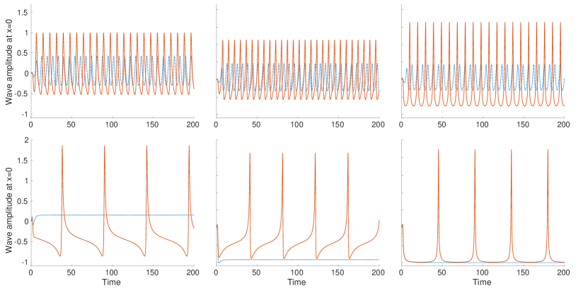
Figure 1: The results of numerical integration of the system 20 and 21, that is time evolution of potential $\phi(x,t)$ at $x=0$ or $A(t)\cos(B(t)+\omega_{k_{0}}t)$. For all plots the values of $\omega_{k_{0}}$, $k_{0}$, $\alpha$ and $\beta$ were set to be equal to 1, $\delta_{A}=0$, and $\gamma$ and $\delta_{B}$ were varied. The right,middle and left columns show plots for phase delay $\delta_{B}$ equals to $\pi/4$, $3\pi/4$ and $\pi/2$ respectively. The top row displays transformation from weakly nonlinear oscillations shown by blue dotted lines for $\gamma=0.75$ to more strongly nonlinear regime (solid line, $\gamma=1.5$ (left and middle) and 2.25 (right)). The bottom row shows the strongest nonlinear spiking–like time evolution of potential $\phi$ (solid line, $\gamma=2.55$ (left and middle) and 2.96 (right)) and its transformation to non-oscillatory (blue dotted line) regime for $\gamma=3$ (time and amplitude units are arbitrary).

Fig. ​​​ 1 shows the results of numerical solution of the system 20 and 21 for several different sets of parameters. The time evolution of highest frequency, longest wave length mode exhibits a variety of types of oscillatory behavior, ranging from slightly nonlinear modified sinusoidal shapes to more nonlinear looking shapes similar to network attributed alpha waves or $\mu$-shaped oscillations [1]. Increase in the level of activation $\gamma$ produces nonlinear signal with spike–like shape of a single neuron firing.

It is interesting that this spiking–like solution of system 20 and 21 appears near the critical point, the oscillatory state undergoes bifurcation and transitions to non-oscillatory regime as $\gamma$ reaches the value above some critical point. To illustrate the reason for this transition we will consider the simplest case of $\delta_{A}=0$ and $\delta_{B}=\pi/2$ (although different $\delta_{A,B}$ values can be used for a similar analysis as well). The non–oscillatory regime can be reached if $dA/dt\rightarrow 0$ and $dB/dt\rightarrow-\omega_{k_{0}}$ as $t\rightarrow\infty$. Then from 20 and 21 one can write that at $t\rightarrow\infty$

$$\gamma A-\omega_{k_{0}}A-2\alpha A^{2}=0,\qquad\beta A\cos B_{0}=-\omega_{k_{0}},$$

where $B_{0}$ is some arbitrary constant phase. Therefore, the non–oscillatory state requires that $\gamma$ satisfies to

$$\gamma=\omega_{k_{0}}\left(1-\frac{2\alpha}{\beta\cos B_{0}}\right).$$ (22)

Hence for

$$\omega_{k_{0}}\left(1-\frac{2\alpha}{\beta}\right)<\gamma<\omega_{k_{0}}\left(1+\frac{2\alpha}{\beta}\right),$$ (23)

the non-oscillatory solution is not possible. The simulations shown in the bottom panels of Fig. ​​​ 1 confirm that the critical $\gamma$ value is indeed 3 when $\omega_{k_{0}}=\alpha=\beta=1$. Similar analysis when $\delta_{A}=\delta_{B}$ gives the critical $\gamma$ value equals to $(2-\cos{(\pi/3)})/\sin{(\pi/3)}\approx 1.732$.

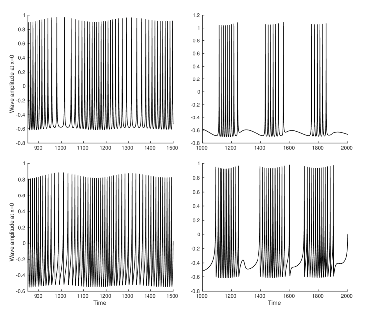
Figure 2: The results of numerical integration of the system 20 and 21 when exponential term was replaced by $I^{nR}$ integrals Universal mechanism of low–frequency brain rhythm formation through nonlinear coupling of high–frequency spiking–like activity with the region of integration set to $50k_{0}<k<1000k_{0}$. For all plots the values of $\omega_{k_{0}}$, $k_{0}$, $\alpha$ and $\beta$ were set to be equal to 1, $\delta_{A}=0$, and $\gamma$ and $\delta_{B}$ were varied. The top and bottom rows show plots for phase delay $\delta_{B}$ equals to $3\pi/4$ and $\pi/2$ respectively. The left column displays modulation of spiking rate for $\gamma=4.5$. The right column shows the nonlinear bursting of spikes for $\gamma=5.1$ (time and amplitude units are arbitrary).

We would like to emphasize that all variety of models used for a description of action potential neuron spikes, starting from the seminal model by Hodgkin and Huxley [15], and finishing with many dynamical integrate–and–fire models of neuron [2], are based on an approximation of several local neuron variables, e.g. membrane currents, gate voltages, etc., and defining the relations between these local properties. Contrary to this and rather unexpectedly, the equation 18 is obtained through an integration of a large number of oscillatory brain wave modes non-resonantly interacting in inhomogeneous anisotropic media and shows spiking pattern solutions emerging as a result of this non–resonant multi–mode interaction rather than as a consequence of empirical fitting of nonlinear model to several locally measured parameters. It is also important that the equation 18 can not be separated into “fast” and “slow” parts as typically required for functioning of “traditional” neuron models. Because of this we would like to reiterate that this equation should not be viewed as a single neuron model and should not be considered as an alternative to any of the single neuron models [16, *Nagumo1962, *pmid7260316]. It describes a mechanism for generation of synchronous spiking activity as a result of a collective input from many non-resonant wave modes. The transition to the synchronous spiking activity occurs in the vicinity of the critical point where a bifurcation from oscillatory to non-oscillatory state happens, thus indirectly supporting the sub-criticality hypothesis [19] of brain operation.

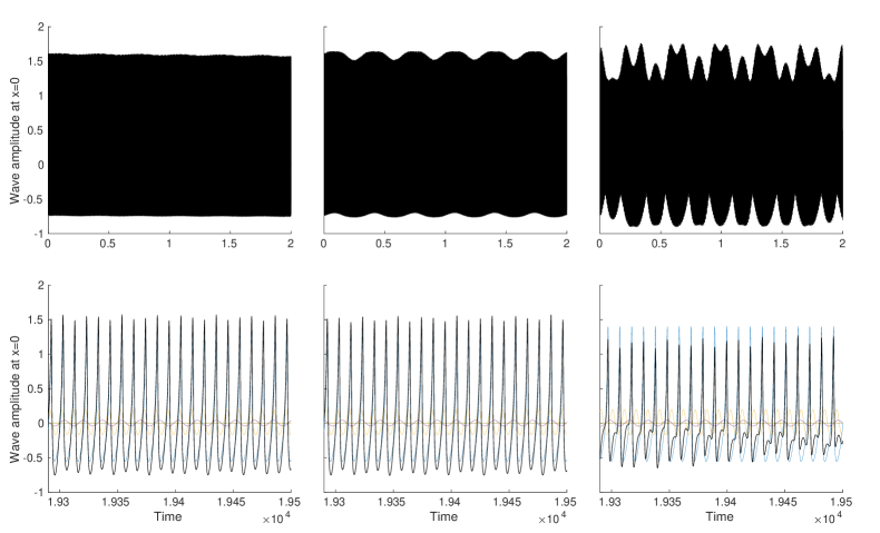
Figure 3: The results of numerical integration of the system Universal mechanism of low–frequency brain rhythm formation through nonlinear coupling of high–frequency spiking–like activity for different values of weak resonant coupling $\lambda=0.001,0.01,0.05$ (left, middle and right columns respectively). For all plots the values of $\omega_{k_{0}}$, $k_{0}$, $\alpha$ and $\beta$ were set to be equal to 1, and $\delta_{A}=\delta_{B}=\delta=3\pi/4$. The value of $\gamma$ is 1.535, that is sufficiently far from the criticality, but nevertheless large enough to modify an effective period for $k_{0}$ mode to be close to that of $k_{1}$. The total potential $\phi$ is plotted with the black and different colors show the oscillations of the individual modes. All plots clearly show emergence of low-frequency component as a result of increase of weak resonant coupling (time and amplitude units are arbitrary).

As a next step we employed more complex expression for the total input from the non-resonant terms by including a sum of all $I^{nR}$ integrals Universal mechanism of low–frequency brain rhythm formation through nonlinear coupling of high–frequency spiking–like activity instead of a single $e^{-i\omega_{k_{0}}t}$ exponent input. Fig. ​​​ 2 shows simulation results for several parameter sets with the same values as were used for plots of Fig. ​​​ 1 ($\omega_{k_{0}}=\beta=k_{0}=1$, $\delta_{A}=0$). The numerical solution shows more complex behavior that includes now modulation of spiking rate with lower frequency and emergence of burst–like train of spikes, effects often observed in different types of neuronal activity [2].

And finally, we considered a model that combines a chain of inputs from nonlinear modes generated due to resonant terms 10 into a set of non-resonant mode equations 18, that results in a system of equations for mode amplitudes $a_{k}$ for $k=k_{0}\dots k_{N}$

$$\frac{d{a_{k_{0}}}}{d{t}} =\frac{a_{k_{0}}}{k_{0}^{2}}\left[\gamma+\frac{\beta}{\Omega|k_{0}|}e^{-i\omega_{k_{0}}t+\delta}a^{*}_{k_{0}}\right]-2\alpha|a_{k_{0}}|a_{k_{0}}$$

$$+\frac{\lambda}{k_{0}^{2}}a^{*}_{k_{1}}a_{k_{2}},$$

$$\frac{d{a_{k_{1}}}}{d{t}} =\frac{a_{k_{1}}}{k_{1}^{2}}\left[\gamma+\frac{\beta}{\Omega|k_{1}|}e^{-i\omega_{k_{1}}t+\delta}a^{*}_{k_{1}}\right]-2\alpha|a_{k_{1}}|a_{k_{1}}$$

$$+\frac{\lambda}{k_{1}^{2}}\left[a_{k_{0}}a_{k_{2}}+a^{*}_{k_{2}}a_{k_{3}}\right],$$

$$\dots$$ (24)

$$\frac{d{a_{k_{n}}}}{d{t}} =\frac{a_{k_{n}}}{k_{n}^{2}}\left[\gamma+\frac{\beta}{\Omega|k_{n}|}e^{-i\omega_{k_{n}}t+\delta}a^{*}_{k_{n}}\right]-2\alpha|a_{k_{n}}|a_{k_{n}}$$

$$+\frac{\lambda}{k_{n}^{2}}\left[a_{k_{n-2}}a^{*}_{k_{n-1}}+a_{k_{n-1}}a_{k_{n+1}}+a^{*}_{k_{n+1}}a_{k_{n+2}}\right],$$

$$\dots$$

$$\frac{d{a_{k_{N}}}}{d{t}} =\frac{a_{k_{N}}}{k_{N}^{2}}\left[\gamma+\frac{\beta}{\Omega|k_{N}|}e^{-i\omega_{k_{N}}t+\delta}a^{*}_{k_{N}}\right]-2\alpha|a_{k_{N}}|a_{k_{N}}$$

$$+\frac{\lambda}{k_{N}^{2}}a_{k_{N-2}}a^{*}_{k_{N-1}},$$

where the parameter $\lambda$ describes the strength of resonant coupling between modes.

We would like to mention two new, rather important, and not entirely obvious features that appear in the nonlinear system Universal mechanism of low–frequency brain rhythm formation through nonlinear coupling of high–frequency spiking–like activity, but absent for phase coupled oscillators [12, *Kuramoto2003]. First, the system Universal mechanism of low–frequency brain rhythm formation through nonlinear coupling of high–frequency spiking–like activity may show multiple critical point transitions corresponding to multiple linear resonant frequencies $\omega_{k_{i}}$ as activation level $\gamma$ increases. Second, sufficiently close to the critical point the strong modification of an effective wave mode frequency by the non–resonant input from multiple wave modes may result in nonlinear resonances with different modes that are not possible for linear waves, thus providing a mechanism for emergence of unexpected oscillations difficult to explain by more simplistic models.

Figs. ​​​ 3 and 4 show results of numerical simulation of the system Universal mechanism of low–frequency brain rhythm formation through nonlinear coupling of high–frequency spiking–like activity, clearly indicating that weak nonlinear resonant coupling between just three modes with frequencies of $\omega_{k_{0}}$, $2\omega_{k_{0}}/(1+\sqrt{5})$ and $2\omega_{k_{0}}/(3+\sqrt{5})$ is capable of explaining an emergence of periodic activity with frequencies up to 100-1000 times lower then the linear frequencies of participating modes. We would like to emphasize again that the system Universal mechanism of low–frequency brain rhythm formation through nonlinear coupling of high–frequency spiking–like activity can not be separated into traditional “slow” and “fast” subsystems, hence the low frequency component can not be explained by a modulation [20] of the “fast” subsystem with oscillations of the “slow” part.

In Fig. ​​​ 3 the high frequency spiking is generated with the level of activation $\gamma=1.535$. This activation level is yet relatively far from criticality but produces spikes with an effective rate that is close to the next linear resonance frequency. The first, second and third columns clearly show that small increase of the resonant coupling (0.001, 0.01 and 0.05 respectively) results in appearance of component with significantly lower frequency.

Fig. ​​​ 4 shows several simulations with the level of activation that is close to criticality for the selected set of parameters in each column. The small resonant coupling $\lambda=0.05$ in this case results in more profound effect of quasiperiodic shift of oscillations back and forth from subcritical to supercritical regimes effectively turning spiking on and off with low frequency. Prediction of the actual period of nonlinear low frequency oscillations from the model parameters, e.g. distances from the critical points and other resonances, phase delays, etc., is an interesting open question that will be considered in future work.

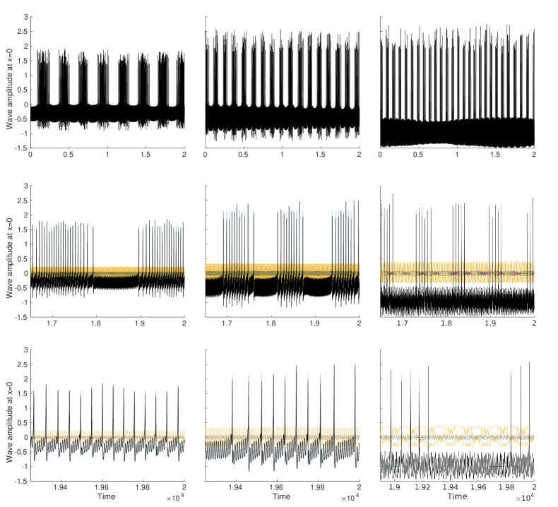
Figure 4: The results of numerical integration of the system Universal mechanism of low–frequency brain rhythm formation through nonlinear coupling of high–frequency spiking–like activity. For all plots the values of $\omega_{k_{0}}$, $k_{0}$, $\alpha$ and $\beta$ were set to be equal to 1 and the resonant coupling $\lambda$ was 0.05. Different values of $\delta$ were again used in real and imaginary parts (as in 20 and 21) with $\delta_{A}=3\pi/4,0,0$, $\delta_{B}=3\pi/4,3\pi/4,\pi/2$ and close to the critical values of $\gamma=1.731,2.575,2,9969$ for the left, middle and right columns respectively. The total potential $\phi$ is plotted with the black and different colors show the oscillations of the individual modes. All plots show that when $\gamma$ is sufficiently close to criticality a week coupling produces jumps from subcritical to supercritical regimes with amazingly regular low–frequency quasiperiodicity (time and amplitude units are arbitrary).

In conclusion, in this paper we used a brain wave model [5] obtained from the general electrostatic form of Maxwell equations in anisotropic and inhomogeneous media for description of interface waves, i.e. waves that propagate in the presence of interfaces (surfaces, boundaries, membranes, transition regions, etc.), to show that the unusual dispersion properties of those waves provide a universal physical mechanism for emergence of low frequencies from high frequency oscillations. The simple quadratic nonlinearity introduced as a coupling source for the wave model allowed the derivation of an equation for a nonlinear form of those waves by taking a limit for a large number of non-resonantly interacting wave modes, which we emphasize is a limit that exists only due to unusual dispersion properties of the waves. The collective input from those non–resonant modes results in nonlinear spiking–like solutions of this equation and an existence of a bifurcation point from oscillatory to non–oscillatory regime. The multi–mode nonlinear system that includes both non-resonant and resonant coupling between multiple modes shows emergence of low frequency modulations as well as strongly nonlinear low frequency quasiperiodic oscillations from subcritical to supercritical regimes. This theory thus provides a basis for relating quantitative tissue microstructural properties (such as anisotropy and inhomogeneity) and measurable larger scale architectural features (e.g, cortical thickness) directly to electrophysiological measurements being performed increasingly sensitive techniques (such as EEG) within a wide range of important basic and clinical research programs.