Sequential estimation of quantiles
with applications to A/B testing and best-arm identification

Abstract

We propose confidence sequences—sequences of confidence intervals which are valid uniformly over time—for quantiles of any distribution over a complete, fully-ordered set, based on a stream of i.i.d. observations. We give methods both for tracking a fixed quantile and for tracking all quantiles simultaneously. Specifically, we provide explicit expressions with small constants for intervals whose widths shrink at the fastest possible $\sqrt{t^{-1}\log\log t}$ rate, along with a non-asymptotic concentration inequality for the empirical distribution function which holds uniformly over time with the same rate. The latter strengthens Smirnov’s empirical process law of the iterated logarithm and extends the Dvoretzky-Kiefer-Wolfowitz inequality to hold uniformly over time. We give a new algorithm and sample complexity bound for selecting an arm with an approximately best quantile in a multi-armed bandit framework. In simulations, our method requires fewer samples than existing methods by a factor of five to fifty.

1 Introduction

A fundamental problem in statistics is the estimation of the location of a distribution based on independent and identically distributed samples. While the mean is the most common measure of location, the median and other quantiles are important alternatives. Quantiles are more robust to outliers and are well-defined for ordinal variables, and sample quantiles exhibit favorable concentration properties, which allow for strong estimation guarantees with minimal assumptions. Beyond estimation, one may choose to actively seek a distribution which maximizes a particular quantile, as in a multi-armed bandit setup, in contrast to the usual setting of finding an arm with maximal mean. In such problems, we wish to find an arm having an approximately best quantile with high probability, while minimizing the total number of samples drawn.

In this paper, we consider the sequential estimation of quantiles and its application to quantile best-arm identification. Specifically, given a stream of i.i.d. observations, we wish to form an estimate of a population quantile, or of all population quantiles, and to continuously update this estimate as more samples are observed to reflect our decreasing uncertainty. Our key tool is the confidence sequence: a sequence of confidence intervals which are guaranteed to contain the desired quantile uniformly over an unbounded time horizon, with the desired coverage probability. For example, if $Q(p)$ denotes the true quantile function and $\widehat{Q}_{t}(p)$ the sample quantile function after having observed $t$ samples (see Section 3 for precise definitions), then for any desired coverage level $\alpha\in(0,1)$, Theorem 1(a) yields the following confidence sequence for the true median, using as confidence bounds a pair of sample quantiles at each time $t$:

$$\mathbb{P}\left(\forall t\in\mathbb{N}:\widehat{Q}_{t}(1/2-u_{t})\leq Q(1/2)\leq\widehat{Q}_{t}(1/2+u_{t})\right)\geq 1-\alpha,\\ \text{where }u_{t}\coloneqq 0.72\sqrt{t^{-1}[1.4\log\log(2.04t)+\log(9.97/\alpha)]}.$$ (1)

Informally, with high probability, the (unknown) population median lies between (observed) sample quantiles slightly above and below the sample median, where “slightly” is determined by a decreasing sequence $u_{t}=\mathcal{O}(\sqrt{t^{-1}\log\log t})$, and moreover, this sequence of upper and lower bounds never fails to contain the true median. In addition to confidence sequences for a fixed quantile, we also derive families of confidence sequences which hold uniformly both over time and over all quantiles. As an example, for any $\alpha\in(0,0.25)$, Corollary 2 yields

$$\mathbb{P}\left(\forall t\in\mathbb{N},p\in(0,1):\widehat{Q}_{t}(p-u_{t})\leq Q(p)\leq\widehat{Q}_{t}(p+u_{t})\right)\geq 1-\alpha,\\ \text{where }u_{t}\coloneqq 0.85\sqrt{t^{-1}[\log\log(et)+0.8\log(1612/\alpha)]}.$$ (2)

The above closed form for $u_{t}$ is one of many possibilities, but Corollary 2 offers better constants, and permits any $\alpha\in(0,1)$, if one is willing to perform numerical root-finding. For example, with $\alpha=0.05$, we can take $u_{t}\coloneqq 0.85\sqrt{t^{-1}(\log\log(et)+8.12)}$ in (2).

Confidence sequences of the form (1) are critical for quantile best-arm algorithms, while those of the form (2) are highly useful for proving corresponding sample complexity bounds. We demonstrate these applications by proving a state-of-the-art sample complexity bound for a new, LUCB-style algorithm. This algorithm outperforms existing algorithms by a large margin in simulation, while the corresponding sample complexity bound matches the best-known rates and requires considerably more technical work than analogous proofs for successive elimination algorithms previously considered.

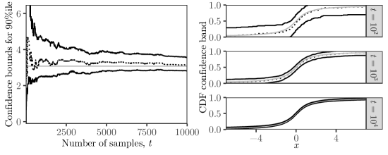
Figure 1: Left: solid lines show upper and lower 95%-confidence sequences using Theorem 1 for the 90%ile of a Cauchy distribution based on one sequence of i.i.d. draws. Grey line shows the true quantile, which lies between the bounds uniformly over all time $t\in\mathbb{N}$ with probability 0.95. Dotted line shows point estimates. Right: solid lines show 95%-confidence bands for the CDF of a Cauchy distribution at three times, $t=$ 100, 1,000, and 10,000, based on one sequence of i.i.d. draws. True CDF, grey, lies between the upper and lower bounds uniformly over all $x\in\mathbb{R}$ and $t\in\mathbb{N}$ with probability 0.95. Dotted line shows empirical CDF.

For a fixed sample size, the celebrated Dvoretzky-Kiefer-Wolfowitz (DKW) inequality (Dvoretzky et al., 1956, Massart, 1990) bounds the uniform-norm deviation of the empirical CDF from the truth with high probability. Corollary 2 follows from Theorem 2, which gives an extension of the DKW inequality that holds uniformly over time. From a theoretical point of view, Theorem 2 gives a non-asymptotic strengthening of the empirical process law of the iterated logarithm (LIL) by Smirnov (1944). From a practical point of view, as Figure 2 illustrates, our time-uniform DKW inequality of Theorem 2 is only about a factor of about two wider in the radius of the high-probability bound, relative to the fixed-sample DKW inequality. This factor grows at a slow $\sqrt{\log\log t}$ rate, so holds over a very long time horizon. Figure 1 illustrates our confidence sequences both for a fixed quantile and for the entire CDF.

Our quantile confidence sequences provide strong guarantees under minimal assumptions while granting the decision-maker a great deal of flexibility. We emphasize the following specific benefits of our confidence sequences:

1. Non-asymptotic and distribution-free: our confidence sequences offer coverage guarantees for all sample sizes in any i.i.d. sampling scenario, regardless of the underlying distribution on any totally ordered space.

2. Unbounded sample size: our methods do not require a final sample size to be chosen ahead of time. Nevertheless, they may be tuned for a planned sample size, but always permit additional sampling.

3. Arbitrary stopping rules: we make no assumptions on the rule used to decide when to stop collecting data and act on given inferences. A user may even perform inference in hindsight based on a previously-seen sample size. That is, the “stopping rule” can be any random time and does not need to be a formal stopping time.

4. Asymptotically zero width: our confidence bounds for the $p$-quantile are based on $p\pm\mathcal{O}(t^{-1/2})$ sample quantiles, ignoring log factors. In this sense, our confidence intervals shrink in width at nearly the same rate as pointwise confidence intervals (see Appendix G for a simple example of pointwise confidence intervals based on the central limit theorem).

1.1 Related work

The pioneering work of Darling and Robbins (1967a) introduced the idea of a confidence sequence, as far as we are aware, and gave a confidence sequence for the median. Their method exploits a standard connection between concentration of quantiles and concentration of the empirical CDF, as does our work, and their method extends trivially to estimating any other fixed quantile. Their confidence sequence was based on the iterated-logarithm, time-uniform bound derived in Darling and Robbins (1967b), and so shrinks in width at the fastest possible $\sqrt{t^{-1}\log\log t}$ rate, like our Theorem 1(a). For the median, their constants are excellent, but the lack of dependence on which quantile is being estimated leads to looseness for tail quantiles, as illustrated in Figure 2. Our results for fixed-quantile estimation yield significantly tighter confidence sequences for tail quantiles (and are also slightly tighter for the median). Schreuder et al. (2020) give another iterated-logarithm-rate confidence sequence for quantiles, a special case of their general method for $M$-estimators.

Our methods for deriving time-uniform, iterated-logarithm CDF and quantile bounds are closely related to the class of methods known as “chaining” in probability theory (Dudley, 1967; Talagrand, 2006; Giné and Nickl, 2015; Boucheron et al., 2013), and similar bounds can be derived using existing chaining techniques. We emphasize our focus on practical constants; our Theorem 2, for example, extends the fixed-sample DKW bound of Massart (1990) to hold uniformly over time at a price of roughly doubling the bound width over many orders of magnitude of time (see Figure 7 in the appendix). Our work is also related to the vast literature on extreme value theory, which contains many results on concentration of extreme sample quantiles (Dekkers and Haan, 1989; Drees, 1998; Drees et al., 2003; Anderson, 1984), though not typically with our focus on time-uniform estimation. Our results can be used to estimate any population quantile, but we place no particular emphasis on the behavior of extreme sample quantiles. If one were particularly interested in extreme tail behavior, e.g., in the distributional properties of the sample maximum, then such references would prove more useful. In addition, general distributional theory of order statistics (empirical quantiles) is well established (Arnold et al., 2008), and specific variance and concentration bounds for order statistics are available (Boucheron and Thomas, 2012). Our methods are rather different in that we always bound population quantiles using sample quantiles, an approach which fits naturally into applications and which yields methods that apply universally without concern for specifics of the underlying distribution.

Shorack and Wellner (1986) give an extensive survey of results for the empirical process $(\widehat{F}_{t}-F)_{t=1}^{\infty}$ for uniform observations, and by extension, the empirical distribution function for any sequence of i.i.d. observations. Of particular relevance is the LIL proved by Smirnov (1944), and the proof given by Shorack and Wellner (1986), based on an improvement of a maximal inequality due to James (1975). This maximal inequality is the key to our sophisticated non-asymptotic empirical process iterated logarithm inequality, Theorem 2. The latter leads to new quantile confidence sequences that are uniform over both quantiles and time which are significantly tighter than the earlier such bounds used for quantile best-arm identification (Szörényi et al., 2015).

The problem of selecting an approximately best arm, as measured by the largest mean, was studied by Even-Dar et al. (2002) and Mannor and Tsitsiklis (2004), who gave an algorithm and sample complexity upper and lower bounds within a logarithmic factor of each other. The best-arm identification or pure exploration problem has received a great deal of attention since then; we mention the influential work of Bubeck et al. (2009) and the proposals of Jamieson et al. (2014), Kaufmann et al. (2016), and Zhao et al. (2016), whose methods included iterated-logarithm confidence sequences for means.

The problem of seeking an arm with the largest median (or other quantile), rather than mean, was first considered by Yu and Nikolova (2013), as far as we are aware. Szörényi et al. (2015) proposed the $(\epsilon,\delta)$-PAC problem formulation that we use, and gave an algorithm with a sample complexity upper bound mirroring that of Even-Dar et al., including the logarithmic factor. Szörényi et al. include a confidence sequence valid over quantiles and time, derived via a union bound applied to the DKW inequality (Dvoretzky et al., 1956, Massart, 1990), similar to the bound used by Darling and Robbins (1968, Theorem 4). Szörényi et al. also analyzed a quantile-based regret-minimization problem, recently studied by Torossian et al. (2019) as well. David and Shimkin (2016) extended the sample complexity of Szörényi et al. to include dependence on the quantile being optimized, while Kalogerias et al. (2020) discuss the $\epsilon=0$ case and give careful consideration to the gap definition appearing in the sample complexity bound. Our procedure is a variant of the LUCB algorithm by Kalyanakrishnan et al. (2012), unlike previous quantile best-arm algorithms; our analysis covers both the $\epsilon=0$ and $\epsilon>0$ cases; we improve the upper bounds of Szörényi et al. by replacing the logarithmic factor by an iterated-logarithm one and removing unnecessary dependence on a unique best arm’s gap; and we achieve considerably better performance than prior algorithms in simulations.

1.2 Paper outline

After an introduction to the conceptual ideas of the paper in Section 2, we present our confidence sequences for estimation of a fixed quantile in Section 3, while Section 4 gives a confidence sequence for all quantiles simultaneously. Section 5 offers a graphical comparison of our bounds with each other and with existing bounds from the literature, as well as advice for tuning bounds in practice. In Section 6, we analyze a new algorithm for quantile $\epsilon$-best-arm identification in a multi-armed bandit, with a state-of-the-art sample complexity bound. We gather proofs in Section 7. Implementations are available online for all confidence sequences presented here (https://github.com/gostevehoward/confseq), along with code to reproduce all plots and simulations (https://github.com/gostevehoward/quantilecs).

2 Warmup: linear boundaries and quantile confidence sequences

Before stating our main results, we first walk through the derivation of a simple confidence sequence for quantiles to illustrate basic techniques. In effect, we spell out the less-known duality between sequential tests and confidence sequences (Howard et al., 2021), analogous to the well-known duality between (standard, fixed time) hypothesis tests and confidence intervals.

Let $(X_{t})_{t=1}^{\infty}$ be a sequence of i.i.d., real-valued observations from an unknown distribution, which we assume is continuous for this section only. For a given $p\in(0,1)$, let $q\in\mathbb{R}$ be such that $\mathbb{P}(X_{1}\leq q)=p$. We wish to sequentially estimate this $p$-quantile, $q$, based on the observations $(X_{t})$. At a high level, our strategy is as follows:

1. We first imagine testing a specific hypothesis $H_{0,x}:q=x$ for some $x\in\mathbb{R}$ at a fixed sample size. Using the aforementioned duality between tests and intervals, we could construct a fixed-sample confidence interval for $q$ consisting of all those values of $x\in\mathbb{R}$ for which we fail to reject $H_{0,x}$.

2. To test $H_{0,x}$ for some fixed $x$, we observe that $H_{0,x}$ is true if and only if the random variables $(1_{X_{t}\leq x})_{t=1}^{\infty}$ are i.i.d. draws from a $\operatorname{Bernoulli}(p)$ distribution. Hence, if the number of samples were fixed in advance, testing $H_{0,x}$ would be equivalent to a standard parametric test: we observe a set of coin flips ($1_{X_{t}\leq x}$), and the null hypothesis states that the bias of this coin is $p$. Inverting this test, as mentioned in the previous point, yields a fixed-sample confidence interval for $q$.

3. Instead of a fixed-sample test, we could apply a sequential hypothesis test, one which can be repeatedly conducted after each new sample $X_{t}$ is observed, with the guarantee that, with the desired, high probability, we will never reject $H_{0,x}$ when it is true. For example, appropriate variants of Wald’s Sequential Probability Ratio Test (SPRT) would suffice. Inverting such a sequential test, we upgrade our fixed-sample confidence interval to a confidence sequence, a sequence of confidence intervals $(\text{CI}_{t})_{t=1}^{\infty}$ which is guaranteed to contain $q$ uniformly over time with high probability: $\mathbb{P}(\forall t:q\in\text{CI}_{t})\geq 1-\alpha$.

To give a rigorous example, consider the random variables $\xi_{t}\coloneqq 1_{X_{t}\leq q}$ for $t\in\mathbb{N}$. We cannot observe $\xi_{t}$ since $q$ is unknown, but we know $(\xi_{t})$ is a sequence of i.i.d. $\operatorname{Bernoulli}(p)$ random variables. A standard (suboptimal, but sufficient for our current exposition) result due to Hoeffding (1963) implies that the centered random variable $\xi_{1}-p$ is sub-Gaussian with variance parameter $1/4$, i.e., $\mathbb{E}e^{\lambda(\xi_{1}-p)}\leq e^{\lambda^{2}/8}$ for any $\lambda\in\mathbb{R}$. Writing $L_{0}\coloneqq 1$ and, for $t\in\mathbb{N}$, defining

$$L_{t}\coloneqq\exp\left\{\lambda\sum_{i=1}^{t}(\xi_{i}-p)-\frac{\lambda^{2}t}{8}\right\},$$ (3)

we observe that $(L_{t})_{t=0}^{\infty}$ is a positive supermartingale for any $\lambda\in\mathbb{R}$ (Darling and Robbins, 1967a; Howard et al., 2020). Then, for any $\alpha\in(0,1)$, Ville’s inequality (Ville, 1939) yields $\mathbb{P}(\exists t\geq 1:L_{t}\geq 1/\alpha)\leq\alpha$, or equivalently,

$$\mathbb{P}\left(\exists t\geq 1:\sum_{i=1}^{t}\xi_{i}\geq tp+\frac{\log\alpha^{-1}}{\lambda}+\frac{\lambda t}{8}\right)\leq\alpha.$$ (4)

The sequence $\left(\frac{\log\alpha^{-1}}{\lambda}+\frac{\lambda t}{8}\right)_{t=1}^{\infty}$ gives a boundary, linear in $t$, which the centered process $\left(\sum_{i=1}^{t}(\xi_{i}-p)\right)_{t=1}^{\infty}$ is unlikely to ever cross. For $\lambda>0$, this bounds the upper deviations of the partial sums $\left(\sum_{i=1}^{t}\xi_{i}\right)_{t=1}^{\infty}$ above their expectations, while for $\lambda<0$, this bounds the lower deviations. Thus by simple rearrangement, and writing

$$u_{t}\coloneqq\frac{\log\alpha^{-1}}{\lambda t}+\frac{\lambda}{8},$$

we infer that $t(p-u_{t})<\sum_{i=1}^{t}\xi_{i}<t(p+u_{t})$ uniformly over all $t\in\mathbb{N}$ with probability at least $1-\alpha$. Observe that $\sum_{i=1}^{t}\xi_{i}$ equals $\left\lvert\left\{i\in[t]:X_{i}\leq q\right\}\right\rvert$, the number of observations up to time $t$ which lie below $q$. So if $\sum_{i=1}^{t}\xi_{i}<t(p+u_{t})$, then we must have $q<X^{t}_{(\lceil t(p+u_{t})\rceil)}$, where $X^{t}_{(k)}$ is the $k$^th order statistic of $X_{1},\dots,X_{t}$. Likewise, $\sum_{i=1}^{t}\xi_{i}>t(p-u_{t})$ implies $q>X^{t}_{(\lfloor t(p-u_{t})\rfloor)}$. In other words, with probability at least $1-\alpha$,

$$q\in\left(X^{t}_{(\lfloor t(p-u_{t})\rfloor)},X^{t}_{(\lceil t(p+u_{t})\rceil)}\right)\quad\text{ simultaneously for all $t\in\mathbb{N}$},$$ (5)

yielding a confidence sequence for the $p$-quantile, $q$. The main drawback of this confidence sequence is that $u_{t}$ does not decrease to zero as $t\uparrow\infty$, so that we do not, in general, expect the confidence sequence to approach zero width as our sample size grows without bound. In other words, the precision of this estimation strategy is unnecessarily limited. The confidence sequences of Section 3 remove this restriction by replacing the $\mathcal{O}(t)$ boundary of (4) with a curved boundary growing at the rate $\mathcal{O}(\sqrt{t\log t})$ or $\mathcal{O}(\sqrt{t\log\log t})$.

3 Confidence sequences for a fixed quantile

We now state our general problem formulation, which removes the assumption that observations are real-valued or from a continuous distribution. Let $(X_{i})_{i=1}^{\infty}$ be a sequence of i.i.d. observations taking values in some complete, totally-ordered set $(\mathcal{X},\leq)$. We shall also make use of the corresponding relations $\geq$, $<$ and $>$ on $\mathcal{X}$. Write $F(x)\coloneqq\mathbb{P}(X_{1}\leq x)$ for the cumulative distribution function (CDF), $F^{-}(x)\coloneqq\mathbb{P}(X_{1}<x)$, and define the empirical versions of these functions $\widehat{F}_{t}(x)\coloneqq t^{-1}\sum_{i=1}^{t}1_{X_{i}\leq x}$ and $\widehat{F}^{-}_{t}(x)\coloneqq t^{-1}\sum_{i=1}^{t}1_{X_{i}<x}$. Define the (standard) upper quantile function as

$$Q(p)\coloneqq\sup\{x\in\mathcal{X}:F(x)\leq p\}$$

and the lower quantile function

$$Q^{-}(p)\coloneqq\sup\{x\in\mathcal{X}:F(x)<p\}.$$

Finally, define the corresponding (plug-in) upper and lower empirical quantile functions $\widehat{Q}_{t}(p)\coloneqq\sup\{x\in\mathcal{X}:\widehat{F}_{t}(x)\leq p\}$ and $\widehat{Q}^{-}_{t}(p)\coloneqq\sup\{x\in\mathcal{X}:\widehat{F}_{t}(x)<p\}$. We extend the empirical quantile functions to hold over domain $p\in\mathbb{R}$ by taking the convention that the supremum of the empty set is $\inf\mathcal{X}$, so that $\widehat{Q}_{t}(p)=\widehat{Q}^{-}_{t}(p)=\inf\mathcal{X}$ for $p<0$ while $\widehat{Q}_{t}(p)=\widehat{Q}^{-}_{t}(p)=\sup\mathcal{X}$ for $p>1$.

Fixing any $p\in(0,1)$ and $\alpha\in(0,1)$, our goal in this section is to give a $(1-\alpha)$-confidence sequence for the true quantiles $Q^{-}(p),Q(p)$ in terms of sample quantiles. In particular, we propose positive, real-valued sequences $l_{t}(p)$ and $u_{t}(p)$ for $t\in\mathbb{N}$, each decreasing to zero as $t\uparrow\infty$, satisfying

$$\mathbb{P}\left(\exists t\in\mathbb{N}:Q^{-}(p)<\widehat{Q}_{t}(p-l_{t}(p))\text{ or }Q(p)>\widehat{Q}^{-}_{t}(p+u_{t}(p))\right) \leq\alpha.$$ (6)

Stated differently, for any $q\in[Q^{-}(p),Q(p)]$, we would have

$$\mathbb{P}\left(\forall t\in\mathbb{N}:q\in[\widehat{Q}_{t}(p-l_{t}(p)),\widehat{Q}^{-}_{t}(p+u_{t}(p))]\right) \geq 1-\alpha.$$ (7)

The sequences $(l_{t}(p),u_{t}(p))_{t=1}^{\infty}$ characterize the lower and upper radii of the confidence intervals in “$p$-space”, before passing through the sample quantile functions $\widehat{Q}_{t}$ and $\widehat{Q}^{-}_{t}$ to obtain final confidence bounds in $\mathcal{X}$. In what follows, we characterize the asymptotic rates of our confidence interval widths in terms of these “$p$-space” widths.

Before stating our confidence sequences, we observe the following lower bound, a straightforward consequence of the law of the iterated logarithm.

Proposition 1 (Quantile confidence sequence lower bound).

For any $p\in(0,1)$ such that $F(Q(p))=p$, if

$$\limsup_{t\to\infty}\frac{u_{t}}{\sqrt{2p(1-p)t^{-1}\log\log t}}<1,$$ (8)

then $\mathbb{P}(\exists t\in\mathbb{N}:Q(p)\geq\widehat{Q}_{t}(p+u_{t}))=1$.

This result is proved in Section C.2. Note that the condition $F(Q(p))=p$ holds for all $p\in(0,1)$ when $F$ is continuous, and holds for at least some $p$ otherwise; more technical effort can be expended to remove this restriction, but we do not do this since the takeaway message is already transparent.

We now propose two confidence sequences. The first has radii given by the function

$$f_{t}(p)\coloneqq 1.5\sqrt{p(1-p)\ell(t)}+0.8\ell(t)\quad\text{where}\quad\ell(t)\coloneqq\frac{1.4\log\log(2.1t)+\log(10/\alpha)}{t}.$$ (9)

This method has the advantage of a closed-form expression with small constants, and evidently $f_{t}(p)\sim\sqrt{3.15p(1-p)t^{-1}\log\log t}$ as $t\to\infty$, matching the lower bound given in Proposition 1 up to the leading constant. Section 7.1 gives a more general version of $f_{t}(p)$ involving several hyperparameters, showing that the leading constant may in fact be brought arbitrarily close to the optimal value of two appearing in Proposition 1, though doing so tends to yield inferior performance in practice. The derivation of $f_{t}(p)$ relies on a method that goes by different names — chaining, “peeling”, or “stitching” — in which we divide time into geometrically-spaced epochs $[\eta^{k},\eta^{k+1})$, and bound the miscoverage event within the $k$^th epoch by a probability which decays like $k^{-s}$, for hyperparameters $\eta,s>1$ described in Section 7.1.

Our second method uses a function $\widetilde{f}_{t}(p)$ which requires numerical root-finding to compute exactly, but has the asymptotic expansion

$$\widetilde{f}_{t}(p)=\sqrt{\frac{p(1-p)}{t}\left[\log\left(\frac{p(1-p)t}{C_{p,r}^{2}\alpha^{2}}\right)+o(1)\right]},\quad\text{where }C_{p,r}\coloneqq\sqrt{2\pi}p(1-p)f_{\beta}\left(p;\frac{r}{1-p},\frac{r}{p}\right),$$ (10)

as $t\to\infty$; here $f_{\beta}(x;a,b)$ denotes the density of the Beta distribution with parameters $a,b$, and $r>0$ is a tuning parameter. The function $\widetilde{f}_{t}(p)$ is described fully in Section 7.1, while we discuss the choice of the tuning parameter $r$ in Section 5 and derive the asymptotic expansion (10) in Section C.1. We note here that as $p$ approaches zero or one, the constant $C_{p,r}$ approaches a constant depending only on $r$, so it does not contribute to dependence on $p$ for tail quantiles. Compared to $f_{t}(p)$, $\widetilde{f}_{t}(p)$ yields confidence interval widths with a slightly worse asymptotic rate of $\mathcal{O}(\sqrt{t^{-1}\log t})$. Even though neither of our methods uniformly dominates the other, the worse rate is usually preferable in practice, as we explore in Section 5. Informally, the reason is that any method with asymptotically optimal rates must be looser at practically relevant sample sizes in order to gain this later tightness, since the overall probability of error of both envelopes can be made arbitrarily close to $\alpha$. The following result shows that both the above methods yield valid confidence sequences for any fixed $p$.

Theorem 1 (Confidence sequence for a fixed quantile).

Taking $f_{t}$ from (9), for any $p\in(0,1)$ and any $\alpha\in(0,1)$, we have

$$\mathbb{P}\left(\exists t\in\mathbb{N}:Q^{-}(p)<\widehat{Q}_{t}\left(p-f_{t}(1-p)\right)\text{ or }Q(p)>\widehat{Q}^{-}_{t}\left(p+f_{t}(p)\right)\right)\leq\alpha.$$ (11)

The same holds with $\widetilde{f}_{t}$ from (45) (asymptotically, (10)) in place of $f_{t}$.

The proof, given in Section 7.1, involves constructing a martingale having bounded increments as a function of the true quantiles $Q^{-}(p)$ and $Q(p)$. Then uniform concentration arguments show that $f_{t}(p)$ and $\widetilde{f}_{t}(p)$ bound the deviations of this martingale from zero, uniformly over time, with high probability. We deduce plausible values for the true quantiles from this high-probability restriction on the values of the martingale.

We could derive a simpler boundary from a sub-Gaussian bound, like that presented in the previous section. For example, one can replace $f_{t}(p)$ or $\widetilde{f}_{t}(p)$ with

$$\sqrt{\frac{t+r}{t^{2}}\log\left(\frac{t+r}{\alpha^{2}r}\right)}$$ (12)

for any $r>0$ (e.g., Howard et al., 2021, eq. 3.7). This bound lacks the appropriate dependence on $\sqrt{p(1-p)}$ indicated in Proposition 1. Our method instead uses “sub-gamma” (for $f_{t}$) and “sub-Bernoulli” (for $\widetilde{f}_{t}$) bounds (Howard et al., 2020) to achieve the correct dependence. The presented bounds are never looser than those obtained by a sub-Gaussian argument, and will be much tighter when $p$ is close to zero or one, as we later illustrate in Figure 2(b).

Having presented our confidence sequences for a fixed quantile, we next present bounds that are uniform over both quantiles and time.

4 Confidence sequences for all quantiles simultaneously

Theorem 1 is useful when the experimenter has decided ahead of time to focus attention on a particular quantile, or perhaps a small number of quantiles (via a union bound). In some cases, however, it may be preferable to estimate all quantiles simultaneously, so that the experimenter may adaptively choose which quantiles to estimate after seeing the data. Equivalently, one may wish to bound the deviations of all sample quantiles uniformly over time, as in our proof of Theorem 3 in Section 6. Recall that for a fixed time $t$ and $\alpha\in(0,1)$, the DKW inequality (Dvoretzky et al., 1956; Massart, 1990) states that

$$\mathbb{P}\left(\left\lVert\widehat{F}_{t}-F\right\rVert_{\infty}>\sqrt{\frac{\log(2/\alpha)}{2t}}\right)\leq\alpha.$$ (13)

In tandem with the implications in (34) of Section 7, the DKW inequality yields

$$\mathbb{P}\left(\exists p\in(0,1):Q^{-}(p)<\widehat{Q}^{-}_{t}(p-l_{t})\text{ or }Q(p)>\widehat{Q}_{t}(p+u_{t})\right)\leq\alpha,$$ (14)

where $l_{t}=u_{t}=\sqrt{\log(2/\alpha)/(2t)}$. In this section, we derive a $(1-\alpha)$-confidence sequence which is valid uniformly over both quantiles and time, based on a function sequence $l_{t}(p),u_{t}(p)$ decreasing to zero pointwise as $t\uparrow\infty$:

$$\mathbb{P}\left(\exists t\in\mathbb{N},p\in(0,1):Q^{-}(p)<\widehat{Q}^{-}_{t}(p-l_{t}(p))\text{ or }Q(p)>\widehat{Q}_{t}(p+u_{t}(p))\right)\leq\alpha.$$ (15)

Our method is based on the following non-asymptotic iterated logarithm inequality for the empirical process $(\widehat{F}_{t}-F)_{t=1}^{\infty}$, which may be of independent interest.

Theorem 2 (Empirical process finite LIL bound).

For any initial time $m\geq 1$ and $C\geq 7$, we have

$$\mathbb{P}\left(\exists t\geq m:\left\lVert\widehat{F}_{t}-F\right\rVert_{\infty}>0.85\sqrt{\frac{\log\log(et/m)+C}{t}}\right)\leq 1612e^{-1.25C}.$$ (16)

Furthermore, for any $A>1/\sqrt{2}$, $C>0$, and $m\geq 1$, we have

$$\mathbb{P}\left(\left\lVert\widehat{F}_{t}-F\right\rVert_{\infty}>A\sqrt{\frac{\log\log(et/m)+C}{t}}\text{ infinitely often}\right)=0.$$ (17)

We give a more detailed result along with the proof in Section 7.2, based on a maximal inequality due to James (1975) and Shorack and Wellner (1986) combined with a union bound over exponentially-spaced epochs. Taking $A$ arbitrarily close to $1/\sqrt{2}$ immediately implies the following asymptotic upper LIL.

Corollary 1 (Smirnov, 1944).

For any (possibly discontinuous) $F$, we have

$$\limsup_{t\to\infty}\frac{\lVert\widehat{F}_{t}-F\rVert_{\infty}}{\sqrt{(1/2)t^{-1}\log\log t}}\leq 1\text{ almost surely}.$$ (18)

A comprehensive overview of results for the empirical process $\sqrt{t}(\widehat{F}_{t}-F)$ can be found in Shorack and Wellner (1986). We mention in particular the law of the iterated logarithm derived by Smirnov (1944) (cf. Shorack and Wellner, 1986, page 12, equation (11)), which says that for continuous $F$, the bound (18) holds with equality, seeing as the lower bound on the $\limsup$ follows directly from the original LIL (Khintchine, 1924) applied to $\widehat{F}_{t}(Q(1/2))$, an average of i.i.d. $\operatorname{Bernoulli}(1/2)$ random variables. Theorem 2 strengthens Smirnov’s asymptotic upper bound to one holding uniformly over time, without costing constant factors in the resulting asymptotic implication.

The following confidence sequence follows immediately from Theorem 2, as detailed in Section C.4.

Corollary 2 (Quantile-uniform confidence sequence I).

For any initial time $m\geq 1$ and $C\geq 7$, letting $g_{t}\coloneqq 0.85\sqrt{t^{-1}(\log\log(et/m)+C)}$, we have

$$\small\mathbb{P}\left(\exists t\geq m,p\in(0,1):Q^{-}(p)<\widehat{Q}^{-}_{t}\left(p-g_{t}\right)\text{ or }Q(p)>\widehat{Q}_{t}\left(p+g_{t}\right)\right)\leq 1612e^{-1.25C}.$$ (19)

For example, take $m=1$ and $C=8.3$, so that $g_{t}=0.85\sqrt{t^{-1}(\log\log(et)+8.3)}$ and

$$\mathbb{P}\left(\exists t\geq 1,p\in(0,1):Q^{-}(p)<\widehat{Q}^{-}_{t}\left(p-g_{t}\right)\text{ or }Q(p)>\widehat{Q}_{t}\left(p+g_{t}\right)\right)\leq 0.05.$$ (20)

Figure 2(a) shows that Corollary 2 yields an improvement over other published methods based on the fixed-time DKW inequality combined with a more naive union bound over time.

Note that $g_{t}$ does not depend on $p$, like the DKW-based fixed-time inequality (14), but this is not ideal for tail quantiles. We describe an alternative “double stitching” method in Theorem 5 of Appendix A which does include such dependence, and yields improved performance for $p$ near zero or one. We demonstrate this performance in Figure 2 of the following section, graphically comparing all of our bounds to visualize their tightness.

5 Graphical comparison of bounds

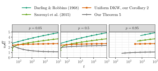
(a) Confidence sequences uniform over both time and quantiles.

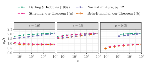
(b) Confidence sequences uniform over time for a fixed quantile.

Figure 2: Plot of upper confidence bound radii $u_{t}$, normalized by $\sqrt{t}$ to facilitate comparison. Each panel shows estimation radius for a different quantile, $p=0.05$, 0.5, and 0.95, respectively. All bounds correspond to two-sided $\alpha=0.05$. Upper row (a) shows confidence sequences valid uniformly over both time and quantiles. Lower row (b) shows confidence sequences valid uniformly over either time for a fixed quantile. In rightmost panels, lines start at the sample size for which the upper confidence bound becomes nontrivial. See Appendix D for details of each bound shown.

Figure 2 compares our four quantile confidence sequences with a variety of alternatives from the literature. In each case, we show the upper confidence bound radius $u_{t}$ which satisfies $\widehat{Q}_{t}(p+u_{t})\geq Q(p)$ with high probability, uniformly over $t$, $p$, or both. Figure 7 in Appendix D includes an additional plot with all bounds together, along with details on all bounds displayed.

Among bounds holding uniformly over both time and quantiles, Corollary 2 and Theorem 5 yield the tightest bounds outside of a brief time window near the start. The bound of Theorem 5 gives $u_{t}$ growing at an $\mathcal{O}(\sqrt{t^{-1}\log t})$ rate for all $p\neq 1/2$, which is worse than that of Corollary 2, but the superior constants of Theorem 5 and its dependence on $p$ give it the advantage in the plotted range. Szörényi et al. (2015) also give a bound which grows as $\mathcal{O}(\sqrt{t^{-1}\log t})$, but with worse constants due to the application of a union bound over individual time steps $t\in\mathbb{N}$. A similar technique was employed by Darling and Robbins (1968, Theorem 4), but using worse constants in the DKW bound, as their work preceded Massart (1990). Finally, Corollary 2 gives an $\mathcal{O}(\sqrt{t^{-1}\log\log t})$ bound which is especially useful for theoretical work, as in our proof of Theorem 3.

Among bounds holding uniformly over time for a fixed quantile, the beta-binomial confidence sequence of Theorem 1(b) performs best over the plotted range, slightly outperforming its iterated-logarithm counterpart from Theorem 1(a). It is evident, though, that the iterated-logarithm bound will become tighter for large enough $t$, thanks to its smaller asymptotic rate. Darling and Robbins (1967a, Section 2) give a similar bound based on a sub-Gaussian uniform boundary, which is only slightly worse than Theorem 1(a) for the median, but substantially worse for $p$ near zero and one.

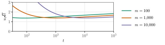
Figure 3: Plot of upper confidence bound radii $u_{t}$, normalized by $\sqrt{t}$ to facilitate comparison, for the confidence sequence of Theorem 1(b) optimized for three different times $m=100$, 1,000, and 10,000, according to (21).

Figure 2 starts at $t=32$ and all bounds have been tuned to optimize for, or start at, $t=32$, in order to ensure a fair comparison. For Theorem 1(a), Corollary 2, and Theorem 5, we simply set $m=32$. For Theorem 1(b), we suggest setting $r$ as follows to optimize for time $t=m$:

$$\frac{r}{p(1-p)}=\frac{m}{-W_{-1}(-\alpha^{2}/e)-1}-1\approx\frac{m}{2\log(\alpha^{-1})+\log\log(e\alpha^{-2})}-1,$$ (21)

where $W_{-1}(x)$ is the lower branch of the Lambert $W$ function, the most negative real-valued solution in $z$ to $ze^{z}=x$, and the second expression uses the asymptotic expansion of $W_{-1}$ near the origin (Corless et al., 1996). See Howard et al. (2021, Proposition 3, Proposition 7, and discussion therein) for details on this choice. Figure 3 illustrates the effect of this choice. The confidence radius $u_{t}$ gets loose very quickly for values of $t$ lower than about $m/2$, but grows quite slowly for values of $t>m$. For this reason, we suggest setting $m$ around the smallest sample size at which inferences are desired.

6 Quantile $\epsilon$-best-arm identification

As an application of our quantile confidence sequences, we present and analyze a novel algorithm for identifying an arm with an approximately optimal quantile in a multi-armed bandit setting. Our problem setup matches that of Szörényi et al. (2015), a slight modification of the standard stochastic multi-armed bandit setting. We assume $K$ arms are available, numbered $k=1,\dots,K$, each corresponding to a distribution $F_{k}$ over the sample space $\mathcal{X}$. At each round, the algorithm chooses any arm $k$ to pull, receiving an independent sample from the distribution $F_{k}$. Write $Q_{k}$ for the upper quantile function on arm $k$, $Q_{k}(p)\coloneqq\sup\{x\in\mathcal{X}:F_{k}(x)\leq p\}$, and $Q^{-}_{k}$ for the lower quantile function. Fixing some $\pi\in(0,1)$, the goal is to stop as soon as possible and, with probability at least $1-\delta$, select an $\epsilon$-optimal arm according to the following definition:

Definition 1.

For $\epsilon\in[0,1-\pi)$, we say arm $k$ is $\epsilon$-optimal if

$$Q^{-}_{k}(\pi+\epsilon)\geq\max_{j\in[K]}Q^{-}_{j}(\pi-\epsilon).$$ (22)

Denote the set of $\epsilon$-optimal arms by

$$\mathcal{A}_{\epsilon}\coloneqq\left\{k\in[K]:Q^{-}_{k}(\pi+\epsilon)\geq\max_{j\in[K]}Q^{-}_{j}(\pi-\epsilon)\right\}.$$

Kalyanakrishnan et al. (2012) introduced the LUCB algorithm for highest mean identification, for which Jamieson and Nowak (2014) gave a simplified analysis in the $\epsilon=0$ case. Both are key inspirations for our QLUCB (Quantile LUCB) algorithm and following sample complexity analysis. Despite being conceptually similar, our analysis faces significantly harder technical hurdles due to the nonlinearity and nonsmoothness of quantiles compared to the (sample and population) mean.

QLUCB proceeds in rounds indexed by $t$. At the start of round $t$, $N_{k,t}$ denotes the number of observations from arm $k$. Write $X_{k,i}$ for the $i$^th observation from arm $k$, and let $\widehat{Q}_{k,t}(p)$ denote the upper sample quantile function for arm $k$ at round $t$,

$$\widehat{F}_{k,t}(x)\coloneqq N_{k,t}^{-1}\sum_{i=1}^{N_{k,t}}1_{X_{k,i}\leq x},\qquad\widehat{Q}_{k,t}(p)\coloneqq\sup\left\{x\in\mathcal{X}:\widehat{F}_{k,t}(x)\leq p\right\},$$ (23)

with an analogous definition of $\widehat{Q}^{-}_{k,t}$. QLUCB requires a sequence $(l_{n}(p),u_{n}(p))$ which yields fixed-quantile confidence sequences, as in (6). Our analysis is based on confidence sequences given by (9), by using $\alpha\equiv 2\delta/K$; the factor of two gives us one-sided instead of two-sided coverage at level $\delta/K$, which is all that is needed. Let

$$f_{t}(p)=1.5\sqrt{p(1-p)\ell(t)}+0.8\ell(t),\text{ where }\ell(t)=\frac{1.4\log\log(2.1t)+\log(5K/\delta)}{t},$$ (24)

similar to (9), and let $l_{t}(p)\coloneqq f_{t}(1-p)$ and $u_{t}(p)\coloneqq f_{t}(p)$. We write $L^{\pi+\epsilon}_{k,t}$ and $U^{\pi-\epsilon}_{k,t}$ for the lower and upper confidence sequences on $Q_{k}(\pi+\epsilon)$ and $Q_{k}(\pi-\epsilon)$, respectively:

$$L^{\pi+\epsilon}_{k,t} \coloneqq\widehat{Q}_{k,t}\left(\pi+\epsilon-l_{N_{k,t}}(\pi+\epsilon)\right),$$ (25)

$$U^{\pi-\epsilon}_{k,t} \coloneqq\widehat{Q}^{-}_{k,t}\left(\pi-\epsilon+u_{N_{k,t}}(\pi-\epsilon)\right).$$ (26)

 

Input target quantile $\pi\in(0,1)$, approximation error $\epsilon\in[0,\pi\wedge(1-\pi))$, and error probability $\delta\in(0,1)$.

Sample each arm once, set $N_{k,1}=1$ for all $k\in[K]$ and set $t=1$.

while $L^{\pi+\epsilon}_{k,t}<\max_{j\neq k}U^{\pi-\epsilon}_{j,t}$ for all $k\in[K]$ do,

     Set $h_{t}\in\operatorname*{arg\,max}_{k\in[K]}L^{\pi+\epsilon}_{k,t}$ and $\mathcal{L}_{t}=\operatorname*{arg\,max}_{k\in[K]\setminus h_{t}}U^{\pi-\epsilon}_{k,t}\subseteq[K]$.

     Sample all arms in $\{h_{t}\}\cup\mathcal{L}_{t}$.

     Set $N_{k,t+1}=N_{k,t}+1\text{ if }k\in\{h_{t}\}\cup\mathcal{L}_{t}$, and $N_{k,t+1}=N_{k,t}$ otherwise.

     Increment $t\leftarrow t+1$.

end while

Output any $k$ such that $L^{\pi+\epsilon}_{k,t}\geq\max_{j\neq k}U^{\pi-\epsilon}_{j,t}$.

 

Figure 4: The QLUCB algorithm samples an arm with highest LCB (time-uniform lower confidence bound) for the $(\pi+\epsilon)$-quantile (called $h_{t}$) and the arm(s) with highest UCB (time-uniform upper confidence bound) for the $\pi$-quantile excluding the former (called $\mathcal{L}_{t}$), as long as the aforementioned LCB and UCB overlap.

QLUCB is described in Figure 4. Its sample complexity is determined by the following quantities, which capture how difficult the problem is based on the sub-optimality of the $\pi$-quantiles of each arm:

$$\Delta_{k} \coloneqq\begin{cases}\sup\left\{\Delta\in[0,\pi\wedge(1-\pi)]:Q^{-}_{k}(\pi+\Delta)\leq\max_{j\in[K]}Q^{-}_{j}(\pi-\Delta)\right\},&\lvert\mathcal{A}_{\epsilon}\rvert>1\text{ or }k\notin\mathcal{A}_{\epsilon},\\ \sup\left\{\Delta\in[0,\pi]:Q^{-}_{k}(\pi-\Delta)>\max_{j\neq k}Q^{-}_{j}(\pi+\Delta_{j})\right\},&\mathcal{A}_{\epsilon}=\{k\}.\end{cases}$$ (27)

To understand (27), it is helpful to consider three cases in turn:

• Consider first a suboptimal arm $k\notin\mathcal{A}_{\epsilon}$. Then $\Delta_{k}$ is given by the first case and captures (informally) how much worse arm $k$ is than some better arm. When arm $k$ is sufficiently sampled relative to $\Delta_{k}$, then with high probabiltiy, the upper confidence bound on $Q^{-}_{k}(\pi-\epsilon)$ will be given by a sample quantile which lies below $Q^{-}_{k}(\pi+\Delta_{k})$, and by the gap definition, this will be smaller than the lower confidence bound on $Q^{-}_{j}(\pi+\epsilon)$ for some other sufficiently-sampled arm $j$. Thus we will be confident that $Q^{-}_{j}(\pi+\epsilon)\geq Q^{-}_{k}(\pi-\epsilon)$, a necessary step to conclude that $j\in\mathcal{A}_{\epsilon}$.

• Suppose there is a unique optimal arm, $\mathcal{A}_{\epsilon}=\{k^{\star}\}$. Then $\Delta_{k^{\star}}$ is given by the second case and captures (again informally) how much better arm $k^{\star}$ is than some “best” suboptimal arm. When arm $k^{\star}$ is sufficiently sampled relative to $\Delta_{k^{\star}}$, then with high probability, the lower confidence bound on $Q^{-}_{k^{\star}}(\pi+\epsilon)$ will be given by a sample quantile which lies above $Q^{-}_{k^{\star}}(\pi-\Delta_{k^{\star}})$, and by the gap definition, this will be larger than upper confidence bound on $Q^{-}_{j}(\pi-\epsilon)$ for any other (suboptimal) sufficiently-sampled arm $j$. So when all arms are sufficiently sampled, we will be able to conclude that $Q^{-}_{k^{\star}}(\pi+\epsilon)\geq Q^{-}_{j}(\pi-\epsilon)$ for all suboptimal arms $j\neq k^{\star}$.

• Suppose there are multiple optimal arms, $\lvert\mathcal{A}_{\epsilon}\rvert>1$. Then $\Delta_{k}$ is given by the first case and must be no larger than $\epsilon$. Because the gap only appears as $\epsilon\vee\Delta_{k}$ in our sample complexity bound, the gap is irrelevant in this case. Informally, we must sample both arms sufficiently that we can determine they are “within $\epsilon$ of each other”, regardless of the actual distance between their quantile functions.

Below, Theorem 3 bounds the sample complexity of QLUCB and shows that it successfully selects an $\epsilon$-optimal arm, both with high probability.

Theorem 3.

For any $\pi\in(0,1)$, $\epsilon\in[0,\pi\wedge(1-\pi))$, and $\delta\in(0,1)$, QLUCB stops with probability one, and chooses an $\epsilon$-optimal arm with probability at least $1-\delta$. Furthermore, with probability at least $1-3\delta$, the total number of samples $T$ taken by QLUCB satisfies

$$T=\mathcal{O}\left(\sum_{k=1}^{K}(\epsilon\vee\Delta_{k})^{-2}\log\left(\frac{K\left\lvert\log\left(\epsilon\vee\Delta_{k}\right)\right\rvert}{\delta}\right)\right).$$ (28)

A recent preprint by Kalogerias et al. (2020, Theorem 8) gave a lower bound for the expected sample complexiy when $\epsilon=0$ of the form $\mathcal{O}(\Delta^{-2}\log\delta^{-1})$, where $\Delta$ is the minimum gap among suboptimal arms. Our bound matches the dependence on $\Delta$ up to a doubly-logarithmic factor, and includes an extra factor of $\log K$. We are not aware of a better upper or lower bound, thus removing the (small) $\log K$ gap remains open. David and Shimkin (2016, Theorem 1) give a lower bound when $\epsilon>0$ of the form $\mathcal{O}(\sum_{k}(\epsilon\vee\widetilde{\Delta}_{k})^{-2}\log\delta^{-1})$ using a slightly different gap definition $\widetilde{\Delta}_{k}$. Our bound holds at $\epsilon=0$ in addition to $\epsilon>0$, Our QLUCB algorithm performs considerably better than existing algorithms in our experiments, including the correct scaling with $\pi$, and we hope that will motivate others to work towards fully matching upper and lower bounds.

Theorem 3 is proved in Section 7.3. In brief, the algorithm can only stop with a sub-optimal arm if one of the confidence sequences $L^{\pi+\epsilon}_{k,t}$ or $U^{\pi-\epsilon}_{k,t}$ fails to correctly cover its target quantile, and Theorem 1 bounds the probability of such an error. Furthermore, Theorem 2 ensures that the confidence bounds converge towards their target quantiles at an $\mathcal{O}(\sqrt{t^{-1}\log\log t})$ rate, with high probability, so that the algorithm must stop after all arms have been sufficiently sampled, and the allocation strategy given in the algorithm ensures we achieve sufficient sampling with the desired sample complexity. While our proof is inspired by Kalyanakrishnan et al. (2012) and Jamieson and Nowak (2014) but significantly extends them. The fact that quantile confidence bounds are determined by the random sample quantile function, rather than simply as deterministic offsets from the sample mean, introduces new difficulties which require novel techniques to overcome.

As an alternative to (24), one may use a one-sided variant of $\widetilde{f}_{t}$ from (45) (Howard et al., 2020, Proposition 7). As seen below, this alternative performs well in practice, though the rate of the sample complexity bound suffers slightly, replacing the $\log\lvert\log(\epsilon\vee\Delta_{k})\rvert$ term with $\lvert\log(\epsilon\vee\Delta_{k})\rvert$.

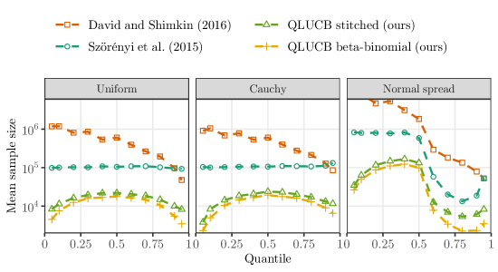
Figure 5: Average sample size for various quantile best-arm identification algorithms based on 64 simulation runs, with $\epsilon=0.025$ and $\pi=0.05,0.1,0.2,\dots,0.8,0.9,0.95$. Left panel shows results for arms with uniform distributions on intervals of length one; middle panel shows arms with Cauchy distributions having unit scale; and right panel shows arms with standard normal distributions except for one, which has a standard deviation of two instead of one. In this last case, the exceptional arm is best for quantiles above $0.53$, while for quantiles below $0.45$, the other arms are all $\epsilon$-optimal. Plot includes Algorithm 2 of David and Shimkin (2016), Algorithm 1 of Szörényi et al. (2015), and our QLUCB algorithm based on two choices of confidence sequence: the stitched confidence sequence (24) based on Theorem 1(a) and a one-sided variant of the beta-binomial confidence sequence, Theorem 1(b).

Figure 5 shows mean sample size from simulations of the quantile $\epsilon$-best-arm identification problem, for variants of QLUCB as well as the QPAC algorithm of Szörényi et al. (2015) and the Doubled Max-Q algorithm of David and Shimkin (2016). In all cases, we have $K=10$ arms and set $\epsilon=0.025$, while $\pi$ ranges between $0.05$ and $0.95$. In the left panel, nine arms have a uniform distribution on $[0,1]$, while one arm is uniform on $[2\epsilon,1+2\epsilon]$. In the middle panel, nine arms have Cauchy distributions with location zero and unit scale, while one arm has location $2(Q(\pi+\epsilon)-Q(\pi))$, where $Q(\cdot)$ is the Cauchy quantile function. This choice ensures that the one exceptional arm is the only $\epsilon$-optimal arm. In the right panel, nine arms have $\mathcal{N}(0,1)$ distributions, while one arm has a $\mathcal{N}(0,2^{2})$ distribution. In this case, the exceptional arm is the only $\epsilon$-optimal arm for $\pi$ larger than approximately 0.53, while it is the only non-$\epsilon$-optimal arm for $\pi$ smaller than approximately 0.45. Between these values, all ten arms are $\epsilon$-optimal.

The results show that QLUCB provides a substantial improvement on QPAC and Doubled Max-Q, reducing mean sample size by a factor of at least five among the cases considered, and often much more, when using the one-sided beta-binomial confidence sequence. As Figure 8 in Appendix F shows, most of the improvement appears to be due to the tighter confidence sequence given by Theorem 1, although the QLUCB sampling procedure also gives a noticeable improvement. The stitched confidence sequence in QLUCB performs similarly to the beta-binomial one, staying within a factor of three across all scenarios and usually within a factor of 1.5.

7 Proofs

We make use of some results from Howard et al. (2020, 2021). We begin with the definitions of sub-Bernoulli, sub-gamma, and sub-Gaussian processes and uniform boundaries:

Definition 2 (Sub-$\psi$ condition).

Let $\smash{(S_{t})_{t=0}^{\infty},(V_{t})_{t=0}^{\infty}}$ be real-valued processes adapted to an underlying filtration $(\mathcal{F}_{t})_{t=0}^{\infty}$ with $\smash{S_{0}=V_{0}=0}$ and $\smash{V_{t}\geq 0}$ for all $t$. For a function $\psi:[0,\lambda_{\max})\to\mathbb{R}$, we say $(S_{t})$ is sub-$\psi$ with variance process $(V_{t})$ if, for each $\lambda\in[0,\lambda_{\max})$, there exists a supermartingale $(L_{t}(\lambda))_{t=0}^{\infty}$ w.r.t. $(\mathcal{F}_{t})$ such that $\mathbb{E}L_{0}(\lambda)\leq 1$ and

$$\exp\left\{\lambda S_{t}-\psi(\lambda)V_{t}\right\}\leq L_{t}(\lambda)\text{ a.s.\ for all }t.$$ (29)

Definition 3.

Given $\smash{\psi:[0,\lambda_{\max})\to\mathbb{R}}$ and $\smash{l_{0}\geq 1}$, a function $\smash{u:\mathbb{R}\to\mathbb{R}}$ is called a sub-$\psi$ uniform boundary with crossing probability $\alpha$ if

$$\mathbb{P}(\exists t\geq 1:S_{t}\geq u(V_{t}))\leq\alpha$$ (30)

whenever $(S_{t})$ is sub-$\psi$ with variance process $V_{t}$.

Definition 4.

We use the following $\psi$ functions in what follows.

1. A sub-Bernoulli process or boundary is sub-$\psi$ with

   $$\psi_{B,g,h}(\lambda)\coloneqq\frac{1}{gh}\log\left(\frac{ge^{h\lambda}+he^{-g\lambda}}{g+h}\right)$$ (31)

   on $0\leq\lambda<\infty$ for some parameters $g,h>0$.

2. A sub-Gaussian process or boundary is sub-$\psi$ with

   $$\psi_{N}(\lambda)\coloneqq\lambda^{2}/2$$ (32)

   on $0\leq\lambda<\infty$.

3. A sub-gamma process or boundary is sub-$\psi$ with

   $$\psi_{G,c}(\lambda)\coloneqq\lambda^{2}/(2(1-c\lambda))$$ (33)

   on $0\leq\lambda<1/(c\vee 0)$ (taking $1/0=\infty$) for some scale parameter $c\in\mathbb{R}$.

The following facts will aid intuition for the true and empirical quantile functions:

• $Q(p)$ and $\widehat{Q}_{t}(p)$ are right-continuous, while $Q^{-}(p)$ and $\widehat{Q}^{-}_{t}(p)$ are left-continuous.

• $\widehat{Q}_{t}(p)$ is the $\lfloor tp\rfloor+1$ order statistic of $X_{1},\dots,X_{t}$, and $\widehat{Q}^{-}_{t}(p)$ is the $\lceil tp\rceil$ order statistic.

• $Q^{-}(p)\leq Q(p)$, and $Q^{-}(p)=Q(p)$ unless the $p$-quantile is ambiguous, that is, $F(x)=F(x^{\prime})=p$ for some $x\neq x^{\prime}$.

• $\widehat{Q}^{-}_{t}(p)\leq\widehat{Q}_{t}(p)$, and $\widehat{Q}^{-}_{t}(p)=\widehat{Q}_{t}(p)$ for all $p\notin\{1/t,2/t,\dots,(t-1)/t\}$.

• $Q^{-}$ is sometimes denoted $F^{-1}$ (e.g., Shorack and Wellner, 1986, p. 3, equation (13)). Our notation seems to improve clarity in the case of ambiguous quantiles.

The functions $\widehat{Q}^{-}_{t}$ and $\widehat{Q}_{t}$ act as “inverses” for $\widehat{F}_{t}$ and $\widehat{F}^{-}_{t}$ in the following sense: for any $x\in\mathcal{X}$ and any $p\in\mathbb{R}$, we have

$$\widehat{F}_{t}(x)\geq p\enskip \Leftrightarrow\enskip x\geq\widehat{Q}^{-}_{t}(p), \widehat{F}_{t}(x)\leq p\enskip \Rightarrow\enskip x\leq\widehat{Q}_{t}(p),$$ (34)

$$\widehat{F}_{t}(x)>p\enskip \Rightarrow\enskip x\geq\widehat{Q}_{t}(p),\qquad\text{and} \widehat{F}^{-}_{t}(x)<p\enskip \Rightarrow\enskip x\leq\widehat{Q}^{-}_{t}(p).$$ (35)

Our strategy in the proof of Theorem 1 will be to construct a martingale $(S_{t}(p))_{t=1}^{\infty}$ which almost surely satisfies

$$\widehat{F}^{-}_{t}(Q(p))\leq p+S_{t}(p)/t\leq\widehat{F}_{t}(Q^{-}(p))$$ (36)

for all $t\in\mathbb{N}$. Applying a time-uniform concentration inequality to bound the deviations of $(S_{t}(p))$, we obtain a time-uniform lower bound $\widehat{F}_{t}(Q^{-}(p))>p-l_{t}(p)$ and a time-uniform upper bound $\widehat{F}^{-}_{t}(Q(p))<p+u_{t}(p)$, both of which hold with high probability. We then invoke the implications in (35) to obtain a confidence sequence for $Q^{-}(p),Q(p)$ of the form (6).

The martingale $(S_{t}(p))$ is defined as follows. Let

$$\pi(p)\coloneqq\begin{cases}0,&F(Q(p))=F^{-}(Q(p)),\\ \frac{p-F^{-}(Q(p))}{F(Q(p))-F^{-}(Q(p))},&F(Q(p))>F^{-}(Q(p)),\end{cases}$$ (37)

noting that $\pi(p)\in[0,1]$ since $F^{-}(Q(p))\leq p\leq F(Q(p))$. Now define $S_{0}(p)=0$ and

$$S_{t}(p)\coloneqq\sum_{i=1}^{t}\left[1_{X_{i}<Q(p)}+\pi(p)1_{X_{i}=Q(p)}-p\right]$$ (38)

for $t\in\mathbb{N}$. When $F(Q(p))=F^{-}(Q(p))$, so that $\mathbb{P}(X_{1}=Q(p))=0$, we have $\widehat{F}^{-}_{t}(Q(p))=p+S_{t}(p)/t=\widehat{F}_{t}(Q(p))$ for all $t\in\mathbb{N}$ a.s. When $F(Q(p))>F^{-}(Q(p))$, we are still assured $\widehat{F}^{-}_{t}(Q(p))\leq p+S_{t}(p)/t\leq\widehat{F}_{t}(Q(p))$ for all $t\in\mathbb{N}$, as desired. In either case, the increments $\Delta S_{t}(p)\coloneqq S_{t}(p)-S_{t-1}(p)$ are i.i.d., mean-zero, and bounded in $[-p,1-p]$ for all $t\in\mathbb{N}$. This key fact allows us to bound the deviations of $S_{t}(p)$ using time-uniform concentration inequalities for Bernoulli random walks.

7.1 Proof of Theorem 1

As defined in (38), the i.i.d. increments of the process $(S_{t}(p))_{t=1}^{\infty}$,

$$S_{t}(p)-S_{t-1}(p)=1_{X_{i}<Q(p)}+\pi(p)1_{X_{i}=Q(p)}-p,$$ (39)

are mean-zero and bounded in $[-p,1-p]$. Fact 1(b) and Lemma 2 of Howard et al. (2020) verify that the process $(S_{t}(p))$ is a sub-Bernoulli process (31) with range parameters $g=p,h=1-p$. Then, defining the intrinsic variance process $V_{t}\coloneqq p(1-p)t$ and

$$\psi(\lambda)\coloneqq\frac{1}{p(1-p)}\log\left(pe^{(1-p)\lambda}+(1-p)e^{-p\lambda}\right),$$ (40)

it is straightforward to verify that the process $\left(\exp\left\{\lambda S_{t}(p)-\psi(\lambda)V_{t}\right\}\right)_{t=1}^{\infty}$ is a supermartingale for all $\lambda\geq 0$. We now construct time-uniform bounds for the process $(S_{t}(p))$ based on the above property:

• Using the fact that a sub-Bernoulli process with range parameters $g=p$ and $h=1-p$ is also sub-gamma with scale $c=(1-2p)/3$, the sequence $f_{t}(p)$ is based on the “polynomial stitched boundary” (Howard et al., 2021, Proposition 1, equation 6, and Theorem 1). That result allows us to fix any $\eta>1$, $s>1$, which control the shape of the confidence radius over time, and $m\geq 1$, the time at which the confidence sequence starts to be tight, and obtain $f_{t}(p)=\mathcal{S}_{p}(t\vee m)/t$ with

  $$\mathcal{S}_{p}(t)\coloneqq\sqrt{k_{1}^{2}p(1-p)t\ell(t)+k_{2}^{2}c_{p}^{2}\ell^{2}(t)}+c_{p}k_{2}\ell(t),\quad\text{where }\begin{cases}\ell(t)\coloneqq s\log\log\left(\frac{\eta t}{m}\right)+\log\left(\frac{2\zeta(s)}{\alpha\log^{s}\eta}\right)\\ k_{1}\coloneqq(\eta^{1/4}+\eta^{-1/4})/\sqrt{2}\\ k_{2}\coloneqq(\sqrt{\eta}+1)/2\\ c_{p}\coloneqq(1-2p)/3.\end{cases}$$ (41)

  The special case given in eq. 9 follows from the choices $\eta=2.04$, $s=1.4$, and $m=1$. Then

  $$\mathbb{P}(\exists t\in\mathbb{N}:S_{t}(p)\geq tf_{t}(p))\leq\alpha/2.$$ (42)

  If we replace $(S_{t}(p))$ with $(-S_{t}(p))$, which is sub-Bernoulli with range parameters $g=1-p$ and $h=p$ and therefore sub-gamma with scale $c=2p-1$, we obtain

  $$\mathbb{P}(\exists t\in\mathbb{N}:S_{t}(p)\leq-tf_{t}(1-p))\leq\alpha/2.$$ (43)

  A union bound yields the two-sided result

  $$\mathbb{P}\left(\exists t\in\mathbb{N}:t^{-1}S_{t}(p)\notin\left(-f_{t}(1-p),f_{t}(p)\right)\right)\leq\alpha.$$ (44)

• The sequence $\widetilde{f}_{t}(p)$ is based on a two-sided beta-binomial mixture boundary drawn from Proposition 7 of Howard et al. (2021). Below, we denote the beta function by $B(a,b)=\int_{0}^{1}u^{a-1}(1-u)^{b-1}\mathop{}\!\mathrm{d}u$. Fix any $r>0$, a tuning parameter, and define

  $$\widetilde{f}_{t}(p) \leavevmode\nobreak\ \coloneqq\leavevmode\nobreak\ \frac{1}{t}\,\sup\left\{s\in\left[0,\frac{r+p(1-p)t}{p}\right):M_{p,r}(s,p(1-p)t)<\frac{1}{\alpha}\right\},$$ (45)

  $$\text{ where \leavevmode\nobreak\ }\leavevmode\nobreak\ M_{p,r}(s,v) \leavevmode\nobreak\ \coloneqq\leavevmode\nobreak\ \frac{1}{p^{v/(1-p)+s}(1-p)^{v/p-s}}\cdot\frac{B\left(\frac{r+v}{p}-s,\frac{r+v}{1-p}+s\right)}{B\left(\frac{r}{p},\frac{r}{1-p}\right)}.$$ (46)

  Then we have

  $$\mathbb{P}\left(\exists t\in\mathbb{N}:t^{-1}S_{t}(p)\notin\left(-\widetilde{f}_{t}(1-p),\widetilde{f}_{t}(p)\right)\right)\leq 1-\alpha.$$ (47)

By construction, $\widehat{F}^{-}_{t}(Q(p))\leq p+S_{t}(p)/t\leq\widehat{F}_{t}(Q^{-}(p))$ for all $t$, so that with (44) we have

$$\mathbb{P}\left(\exists t\in\mathbb{N}:\widehat{F}_{t}(Q^{-}(p))\leq p-f_{t}(1-p)\text{ or }\widehat{F}^{-}_{t}(Q(p))\geq p+f_{t}(p)\right)\leq\alpha.$$ (48)

We now use the implications in (35) to conclude

$$\mathbb{P}\left(\exists t\in\mathbb{N}:Q^{-}(p)<\widehat{Q}_{t}\left(p-f_{t}(1-p)\right)\text{ or }Q(p)>\widehat{Q}^{-}_{t}\left(p+f_{t}(p)\right)\right)\leq\alpha,$$ (49)

which is the desired conclusion. The same conclusion follows for $\widetilde{f}$ by using (47) in place of (44). ∎

We remark that (49) implies that the running intersection of confidence intervals also yields a valid confidence sequence: for any $q\in[Q^{-}(p),Q(p)]$, we have

$$\mathbb{P}\left(\forall t\in\mathbb{N}:q\in\left[\max_{s\leq t}\widehat{Q}_{s}\left(p-f_{s}(1-p)\right),\min_{s\leq t}\widehat{Q}^{-}_{s}\left(p+f_{s}(p)\right)\right]\right) \geq 1-\alpha.$$ (50)

This intersection yields smaller confidence intervals. However, on the miscoverage event of probability $\alpha$, or if the assumption of i.i.d. observations is violated, then the intersection method may lead to an empty confidence interval. This can be viewed as a benefit, as an empty confidence interval is evidence of problematic assumptions. In such cases, however, it may also lead to misleadingly small, but not empty, confidence intervals, which may be harder to detect.

7.2 Proof of Theorem 2

We prove the following more general result:

Theorem 4.

For any $m\geq 1$, $A>1/\sqrt{2}$, and $C>0$, we have

$$\mathbb{P}\left(\exists t\geq m:\left\lVert\widehat{F}_{t}-F\right\rVert_{\infty}>A\sqrt{\frac{\log\log(et/m)+C}{t}}\right)\\ \leq\alpha_{A,C}\coloneqq\inf_{\begin{subarray}{c}\eta\in(1,2A^{2}),\\ \gamma(A,C,\eta)>1\end{subarray}}4e^{-\gamma^{2}(A,C,\eta)C}\left(1+\frac{1}{(\gamma^{2}(A,C,\eta)-1)\log\eta}\right),$$ (51)

where $\gamma(A,C,\eta)\coloneqq\sqrt{2/\eta}\left(A-\sqrt{2(\eta-1)/C}\right)$. Furthermore,

$$\mathbb{P}\left(\left\lVert\widehat{F}_{t}-F\right\rVert_{\infty}>A\sqrt{t^{-1}(\log\log(et/m)+C)}\text{ infinitely often}\right)=0.$$ (52)

To better understand the quantity $\alpha_{A,C}$, note that any value of $\eta\in(1,2A^{2})$ satisfying $\gamma(A,C,\eta)$ gives an upper bound for $\alpha_{A,C}$. For fixed $A$, any value $\eta\in(1,2A^{2})$ is feasible for sufficiently large $C$, while for fixed $C$, any value $\eta>1$ is feasible for sufficiently large $A$. In either case, $\gamma^{2}(A,C,\eta)\sim 2A^{2}/\eta$ as $A\to\infty$ or $C\to\infty$, which yields $\log\alpha_{A,C}=\mathcal{O}(-A^{2}C)$, as may be expected from a typical exponential concentration bound.

To obtain the special case stated in in Theorem 2, take $A=0.85$ and any $C\geq 7$, and observe that the value $\eta=1.01$ ensures that $\gamma^{2}(0.85,C,1.01)\geq 1.25$ and is thus feasible for the right-hand side of (51).

Our proof is based on inequality 13.2.1 of Shorack and Wellner (1986, p. 511) (cf. James, 1975). We repeat the following special case; here $(\cdot)_{\pm}$ denotes that we may take either the positive part of $(\cdot)$ on both sides of the inequality, or the negative part on both sides.

Lemma 1 (Shorack and Wellner, 1986, Inequality 13.2.1).

Fix $\lambda>0$, $\beta\in(0,1)$, and $\eta>1$ satisfying $(1-\beta)^{2}\lambda^{2}\geq 2(\eta-1)$. Then for all integers $n^{\prime}\leq n^{\prime\prime}$ having $n^{\prime\prime}/n^{\prime}\leq\eta$, we have

$$\mathbb{P}\left(\max_{n^{\prime}\leq t\leq n^{\prime\prime}}\left\lVert\sqrt{t}(\widehat{F}_{t}-F)_{\pm}\right\rVert_{\infty}>\lambda\right)\leq 2\mathbb{P}\left(\left\lVert\sqrt{n^{\prime\prime}}(\widehat{F}_{n^{\prime\prime}}-F)_{\pm}\right\rVert_{\infty}>\frac{\beta\lambda}{\sqrt{\eta}}\right).$$ (53)

Now fix any $\eta\in(1,2A^{2})$ satisfying $\gamma(A,C,\eta)>1$, and for $k=0,1,\dots$, define the event

$$\mathcal{A}_{k}^{\pm}\coloneqq\left\{\exists t\in[m\eta^{k},m\eta^{k+1}):\left\lVert(\widehat{F}_{t}-F)_{\pm}\right\rVert_{\infty}>A\sqrt{\frac{\log\log(e\eta^{k})+C}{t}}\right\}.$$ (54)

On the one hand, we have

$$\left\{\exists t\geq m:\left\lVert\widehat{F}_{t}-F\right\rVert_{\infty}>\frac{g_{t}}{t}\right\} =\bigcup_{k\in\mathbb{Z}_{\geq 0}}\left\{\exists t\in[m\eta^{k},m\eta^{k+1}):\left\lVert\widehat{F}_{t}-F\right\rVert_{\infty}>\frac{g_{t}}{t}\right\}$$ (55)

$$\subseteq\bigcup_{k\in\mathbb{Z}_{\geq 0}}\left(\mathcal{A}_{k}^{+}\cup\mathcal{A}_{k}^{-}\right).$$ (56)

On the other hand, we will show that, for each $k\geq 0$, the conditions of Lemma 1 are satisfied with $\lambda\coloneqq A\sqrt{\log\log(e\eta^{k})+C}$ and $\beta\coloneqq 1-\sqrt{2(\eta-1)/(A^{2}C)}=\gamma(A,C,\eta)\sqrt{\eta/(2A^{2})}$. It is clear that $\beta\in(0,1)$ since $A$, $C$, $\eta$, and $\gamma(A,C,\eta)$ are all required to be positive. Also,

$$2(\eta-1)=(1-\beta)^{2}A^{2}C\leq(1-\beta)^{2}A^{2}(\log\log(e\eta^{k})+C)=(1-\beta)^{2}\lambda^{2},\quad\forall k\geq 0.$$ (57)

Hence, for each $k$, Lemma 1 implies

$$\mathbb{P}(\mathcal{A}_{k}^{\pm})\leq 2\mathbb{P}\left(\left\lVert\sqrt{\lfloor\eta^{k+1}\rfloor}(\widehat{F}_{\lfloor\eta^{k+1}\rfloor}-F)_{\pm}\right\rVert_{\infty}>\frac{\beta A\sqrt{\log\log(e\eta^{k})+C}}{\sqrt{\eta}}\right).$$ (58)

Applying the one-sided DKW inequality (Massart, 1990, Theorem 1) then yields

$$\mathbb{P}(\mathcal{A}_{k}^{\pm})\leq 2\exp\left\{-\frac{2c^{2}A^{2}(\log\log(et_{k})+C)}{\eta}\right\}=\frac{2e^{-\gamma^{2}(A,C,\eta)C}}{(1+k\log\eta)^{\gamma^{2}(A,C,\eta)}}.$$ (59)

Since $\gamma(A,C,\eta)>1$, a union bound yields

$$\mathbb{P}\left(\bigcup_{k\in\mathbb{N}}\left(\mathcal{A}_{k}^{+}\cup\mathcal{A}_{k}^{-}\right)\right) \leq 4e^{-\gamma^{2}(A,C,\eta)C}\sum_{k=0}^{\infty}\frac{1}{(1+k\log\eta)^{\gamma^{2}(A,C,\eta)}}$$ (60)

$$\leq 4e^{-\gamma^{2}(A,C,\eta)C}\left(1+\frac{1}{(\gamma^{2}(A,C,\eta)-1)\log\eta}\right),$$ (61)

after bounding the sum by an integral. Combining (56) with (61), we conclude

$$\mathbb{P}\left(\exists t\geq m:\left\lVert\widehat{F}_{t}-F\right\rVert_{\infty}>\frac{g_{t}}{t}\right)\leq 4e^{-\gamma^{2}(A,C,\eta)C}\left(1+\frac{1}{(\gamma^{2}(A,C,\eta)-1)\log\eta}\right).$$ (62)

We note that Theorem 1 of Massart (1990) requires that the tail probability bound in (59) is less than $1/2$. If this is not true, however, then our final tail probability will be at least one, so that the result holds vacuously. This completes the proof of the first part of the theorem.

To obtain the final claim, (52), note that the calculations in (59) and (61), together with the first Borel-Cantelli lemma, imply $\mathbb{P}(A^{+}_{k}\text{ or }A^{-}_{k}\text{ infinitely often})=0$. ∎

7.3 Proof of Theorem 3

Recall that the set of $\epsilon$-optimal arms is denoted by

$$\mathcal{A}_{\epsilon}\coloneqq\left\{k\in[K]:Q^{-}_{k}(\pi+\epsilon)\geq\max_{j\in[K]}Q^{-}_{j}(\pi-\epsilon)\right\}.$$

First, we prove that if QLUCB stops, it selects an $\epsilon$-optimal arm with probability at least $1-\delta$. Choose any $k^{\star}\in\operatorname*{arg\,max}_{k\in[K]}Q^{-}_{k}(\pi-\epsilon)$, an arm with optimal $(\pi-\epsilon)$-quantile, and write $q^{\star}\coloneqq Q^{-}_{k^{\star}}(\pi-\epsilon)$ for the corresponding optimum quantile value. By our choice of $u_{n}$ and $l_{n}$ to give one-sided coverage at level $\delta/K$, the proof of Theorem 1 and a union bound show that

$$\mathbb{P}\left(\exists t\in\mathbb{N}\text{ and }k\neq k^{\star}:U^{\pi-\epsilon}_{k^{\star},t}<q^{\star}\text{ or }L^{\pi+\epsilon}_{k,t}>Q^{-}_{k}(\pi+\epsilon)\right)\leq\delta.$$ (63)

Suppose QLUCB stops at time $T$ with some arm $k\in\mathcal{A}_{\epsilon}^{c}$, so that $Q^{-}_{k}(\pi+\epsilon)<q^{\star}$. Then it must be true that $L^{\pi+\epsilon}_{k,T}\geq U^{\pi-\epsilon}_{k^{\star},T}$, which implies that $L^{\pi+\epsilon}_{k,T}>Q^{-}_{k}(\pi+\epsilon)$ or $U^{\pi-\epsilon}_{k^{\star},T}<q^{\star}$ must hold. But (63) shows that this can only occur on an event of probability at most $\delta$. So with probability at least $1-\delta$, QLUCB can only stop with an $\epsilon$-optimal arm.

Next, we prove that QLUCB stops with probability one and obeys the sample complexity bound (28) with probability at least $1-3\delta$. We first address the case when $\lvert\mathcal{A}_{\epsilon}\rvert>1$ so that $\Delta_{k}$ is given by (27) for all $k$; we consider the case $\lvert\mathcal{A}_{\epsilon}\rvert=1$ at the end. Let

$$g_{n}\coloneqq 0.85\sqrt{n^{-1}\left(\log\log(en)+0.8\log\left(\frac{1612K}{\delta}\right)\right)},$$ (64)

for $n\in N$. We choose this quantity to eventually control the deviations of $\widehat{Q}_{k,t}(p)$ and $\widehat{Q}^{-}{k,t}(p)$ from $Q^{-}_{k}(p)$ and $Q_{k}(p)$ uniformly over $k$, $t$ and $p$, via Corollary 2. For each $k\in[K]$, define

$$\tau_{k}\coloneqq\min\left\{n\in\mathbb{N}:g_{n}+[u_{n}(\pi)\vee l_{n}(\pi+\epsilon)]<\Delta_{k}\vee\epsilon\right\}.$$ (65)

We will show that, once each arm has been sampled in $\mathcal{L}_{t}$ at least $2\tau_{k}$ times, the confidence bounds are sufficiently well-behaved to ensure that QLUCB must stop, on a “good” event with probability at least $1-3\delta$. This will imply that QLUCB stops after no more than $2\sum_{k=1}^{K}\tau_{k}$ rounds on the “good” event, and this sum has the desired rate.

Define the “bad” event at time $t$, $\mathcal{B}_{t}=\mathcal{B}^{1}_{t}\cup\mathcal{B}^{2}_{t}$, where

$$\mathcal{B}^{1}_{t} \coloneqq\left\{\exists k\in[K]:U^{\pi-\epsilon}_{k,t}<Q_{k}(\pi-\epsilon)\text{ or }L^{\pi+\epsilon}_{k,t}>Q^{-}_{k}(\pi+\epsilon)\right\},\text{\leavevmode\nobreak\ and }$$ (66)

$$\mathcal{B}^{2}_{t} \coloneqq\left\{\exists k\in[K],p\in(0,1):\widehat{Q}_{k,t}(p)<Q_{k}(p-g_{N_{k,t}})\text{ or }\widehat{Q}^{-}_{k,t}(p)>Q^{-}_{k}(p+g_{N_{k,t}})\right\}.$$ (67)

We exploit our previous results to bound the probability that $\mathcal{B}_{t}$ ever occurs:

Lemma 2.

$\mathbb{P}\left(\cup_{t=1}^{\infty}\mathcal{B}_{t}\right)\leq 3\delta$.

Proof.

First, by the definitions of $U^{\pi-\epsilon}_{k,t},L^{\pi+\epsilon}_{k,t}$ and our choices of $u_{n},l_{n}$, the proof of Theorem 1(a) yields

$$\mathbb{P}\left(\bigcup_{t=1}^{\infty}\mathcal{B}^{1}_{t}\right)\leq 2\delta.$$ (68)

For $\mathcal{B}^{2}_{t}$, we invoke Corollary 2. Our choice of $C=0.8\log(1612K^{2}/(\delta(K-1)))$ ensures that $\alpha_{0.85,C}\leq(K-1)\delta/K^{2}$, noting that $K\geq 2$ implies $C>7$ as required in (2). Hence, by a union bound,

$$\mathbb{P}\left(\bigcup_{t=1}^{\infty}\mathcal{B}^{2}_{t}\right)\leq\delta.$$ (69)

Combining (68) with (69) via a union bound, we have $\mathbb{P}(\cup_{t=1}^{\infty}\mathcal{B}_{t})\leq 3\delta$ as desired. ∎

The following lemma verifies that an arm’s confidence bounds are well-behaved, in a specific sense, once the arm has been sampled $\tau_{j}$ times and $\mathcal{B}^{2}_{t}$ does not occur. We use the notation $a_{+}\coloneqq\max(0,a)$.

Lemma 3.

For any $t\in\mathbb{N}$ and $j,k\in[K]$, on $(B^{2}_{t})^{c}$, if $N_{k,t}\geq\tau_{j}$, then

$$U^{\pi-\epsilon}_{k,t} \leq Q^{-}_{k}(\pi+(\Delta_{j}-\epsilon)_{+}),\quad\text{and}$$ (70)

$$L^{\pi+\epsilon}_{k,t} \geq Q_{k}(\pi-(\Delta_{j}-\epsilon)_{+}).$$ (71)

Proof.

From the definition of $U^{\pi-\epsilon}_{k,t}$,

$$U^{\pi-\epsilon}_{k,t}=\widehat{Q}^{-}_{k,t}(\pi-\epsilon+u_{N_{k,t}}(\pi-\epsilon))\leq Q^{-}_{k}(\pi-\epsilon+u_{N_{k,t}}(\pi-\epsilon)+g_{N_{k,t}}),$$ (72)

since we are on $(\mathcal{B}^{2}_{t})^{c}$. Then since $N_{k,t}\geq\tau_{j}$,

$$Q^{-}_{k}(\pi-\epsilon+u_{N_{k,t}}(\pi-\epsilon)+g_{N_{k,t}})\leq Q^{-}_{k}(\pi-\epsilon+(\Delta_{j}\vee\epsilon))=Q^{-}_{k}(\pi+(\Delta_{j}-\epsilon)_{+}).$$ (73)

An analogous argument shows the second conclusion:

$$L^{\pi+\epsilon}_{k,t}=\widehat{Q}_{k,t}(\pi+\epsilon-l_{N_{k,t}}(\pi+\epsilon)) \geq Q_{k}(\pi+\epsilon-l_{N_{k,t}}(\pi+\epsilon)-g_{N_{k,t}})$$ (74)

$$\geq Q_{k}(\pi+\epsilon-(\Delta_{j}\vee\epsilon))=Q_{k}(\pi-(\Delta_{j}-\epsilon)_{+}).$$ (75)

∎

The next three lemmas will show that, once an arm in $\mathcal{L}_{t}$ has been sufficiently sampled, QLUCB must stop. The easier case is when an arm’s gap is small, $\Delta_{k}<\epsilon$.

Lemma 4.

For any $t\in\mathbb{N}$ and $k\in[K]$ with $\Delta_{k}<\epsilon$, on $(B^{2}_{t})^{c}$, if $N_{k,t}\geq\tau_{k}$, then $L^{\pi+\epsilon}_{h_{t},t}\geq U^{\pi-\epsilon}_{k,t}$.

Proof.

Our choice of $h_{t}$ ensures $L^{\pi+\epsilon}_{h_{t},t}\geq L^{\pi+\epsilon}_{k,t}$, while (70) and (71) show that

$$L^{\pi+\epsilon}_{k,t}\geq Q_{k}(\pi)\geq Q^{-}_{k}(\pi)\geq U^{\pi-\epsilon}_{k,t}.$$ (76)

∎

To handle arms with $\Delta_{k}\geq\epsilon$, we associate with each arm $k$ an arm $g(k)$ which satisfies $Q^{-}_{k}(\pi+\Delta_{k})\leq Q_{g(k)}(\pi-\Delta_{k})$. Some such arm must exist by the definition of $\Delta_{k}$ and the fact that $Q^{-}$ is left-continuous while $Q$ is right-continuous. We first show that, when an arm $k\in\mathcal{L}_{t}$ with $\Delta_{k}\geq\epsilon$ has been sufficiently sampled, we must also sample $g(k)$:

Lemma 5.

For any $t\in\mathbb{N}$ and $k\in[K]$ with $\Delta_{k}\geq\epsilon$, on $B_{t}^{c}$, if $N_{k,t}\geq\tau_{k}$, then $U^{\pi-\epsilon}_{g(k),t}\geq U^{\pi-\epsilon}_{k,t}$.

Proof.

Bound (70) and our choice of $g(k)$ ensure

$$U^{\pi-\epsilon}_{k,t}\leq Q^{-}_{k}(\pi+\Delta_{k})\leq Q_{g(k)}(\pi-\Delta_{k}).$$ (77)

But $\Delta_{k}\geq\epsilon$, so $Q_{g(k)}(\pi-\Delta_{k})\leq Q_{g(k)}(\pi-\epsilon)$, and the latter is upper bounded by $U^{\pi-\epsilon}_{g(k),t}$ since we are on $(B^{1}_{t})^{c}$. ∎

Finally, we show that once arms $k\in\mathcal{L}_{t}$ and $g(k)$ have both been sufficiently sampled, we must stop.

Lemma 6.

For any $t\in\mathbb{N}$ and $k\in[K]$ with $\Delta_{k}\geq\epsilon$, on $B_{t}^{c}$, if $N_{k,t}\geq\tau_{k}$ and $N_{g(k),t}\geq\tau_{k}$, then $L^{\pi+\epsilon}_{h_{t},t}\geq U^{\pi-\epsilon}_{k,t}$.

Proof.

As in (77), we have

$$U^{\pi-\epsilon}_{k,t}\leq Q_{g(k)}(\pi-\Delta_{k})\leq Q_{g(k)}(\pi-(\Delta_{k}-\epsilon)_{+}).$$ (78)

But since $N_{g(k),t}\geq\tau_{k}$, (71) implies

$$Q_{g(k)}(\pi-(\Delta_{k}-\epsilon)_{+})\leq L^{\pi+\epsilon}_{g(k),t}\leq L^{\pi+\epsilon}_{h_{t},t}$$ (79)

by our choice of $h_{t}$. ∎

We combine the preceding lemmas in the following key result. Write $M_{k,t}=\sum_{s=1}^{t}1_{k\in\mathcal{L}_{s}}$ and note that $N_{k,t}\geq M_{k,t}$ since we sample every arm in $\mathcal{L}_{t}$ at time $t$.

Lemma 7.

For any $t\in\mathbb{N}$, on $\mathcal{B}_{t}^{c}$, if $M_{k,t}\geq 2\tau_{k}$ for any $k\in\mathcal{L}_{t}$, then QLUCB must stop at time $t$.

Proof.

If $\Delta_{k}<\epsilon$ then the conclusion follows immediately from Lemma 4. If $\Delta_{k}\geq\epsilon$, then Lemma 5 implies $N_{g(k),t}\geq M_{k,t}-\tau_{k}$, since once $M_{k,t}\geq\tau_{k}$, we must have $U_{g(k),t}\geq U_{k,t}$ so that either $g(k)=h_{t}$ or $g(k)\in\mathcal{L}_{t}$ whenever $k\in\mathcal{L}_{t}$. Thus when $M_{k,t}\geq 2\tau_{k}$, we must have $N_{g(k),t}\geq\tau_{k}$ and the conclusion follows from Lemma 6. ∎

We can now show that QLUCB stops after no more than $4\sum_{k=1}^{K}\tau_{k}$ samples with probability at least $1-3\delta$. On $\mathcal{B}_{t}^{c}$, Lemma 7 allows us to write

$$T \leq\sum_{t=1}^{\infty}(1+\lvert\mathcal{L}_{t}\rvert)1\{M_{k,t}<2\tau_{k}\text{ for all }k\in\mathcal{L}_{t}\}$$ (80)

$$\leq 2\sum_{t=1}^{\infty}\sum_{k=1}^{K}1\{k\in\mathcal{L}_{t}\text{ and }M_{k,t}<2\tau_{k}\}$$ (81)

$$\leq 4\sum_{k=1}^{K}\tau_{k},$$ (82)

by the definition of $M_{k,t}$. Hence $\mathbb{P}(T\leq 4\sum_{k=1}^{K}\tau_{k})\geq 1-\mathbb{P}(\cup_{t=1}^{\infty}\mathcal{B}_{t})\geq 1-3\delta$ using Lemma 2. It remains to show that $T<\infty$ a.s., and to show that $\sum_{k=1}^{K}\tau_{k}$ has the desired rate.

First, Corollary 1 of Howard et al. (2021) implies that $\mathbb{P}(\mathcal{B}^{1}_{t}\text{ infinitely often})=0$, while Theorem 2 implies $\mathbb{P}(\mathcal{B}^{2}_{t}\text{ infinitely often})=0$. So, with probability one, there exists $t_{0}$ such that $\mathcal{B}_{t}$ occurs for no $t\geq t_{0}$, and the above calculations show that $T\leq t_{0}+4\sum_{k=1}^{K}\tau_{k}$. We conclude $T<\infty$ almost surely.

Second, to show that $\sum_{k=1}^{K}\tau_{k}$ has the rate given in (28), we use the following lemma, which bounds the time for an iterated-logarithm confidence sequence radius to shrink to a desired size.

Lemma 8.

Suppose $(a_{n}(C))_{n\in\mathbb{N}}$ is a real-valued sequence for each $C>0$ satisfying $a_{n}=\mathcal{O}(\sqrt{n^{-1}(\log\log n+C)})$ as $n,C\uparrow\infty$. Then

$$\min\left\{n\in\mathbb{N}:a_{n}(C)\leq x\right\}=\mathcal{O}\left(\frac{\log\log x^{-1}+C}{x}\right)\quad\text{as }x\downarrow 0,C\uparrow\infty.$$ (83)

Proof.

Our condition on $a_{n}(C)$ implies, for small enough $x$ and large enough $C$,

$$\min\left\{n\in\mathbb{N}:a_{n}(C)\leq x\right\}\leq\min\left\{n\in\mathbb{N}:\frac{\log(1+\log n)+C}{n}\leq\frac{x^{2}}{A^{2}}\right\}\eqqcolon t(x).$$ (84)

Use $\log(1+x)\leq x$ to see that $\log x=2\log\sqrt{x}\leq 2(\sqrt{x}-1)$, and that

$$\frac{\log(1+\log n)+C}{n}\leq\frac{\log n+C}{n}\leq\frac{2}{\sqrt{n}}+\frac{C-2}{n}\leq\frac{C}{\sqrt{n}},$$ (85)

as $n\geq\sqrt{n}$. So $n\geq C^{2}A^{4}/x^{4}$ implies that $(\log(1+\log n)+C)/n\leq x^{2}/A^{2}$, and we must have $t(x)\leq C^{2}A^{4}/x^{4}+1$. Hence we may write

$$t(x)=\min\left\{n\in\mathbb{N}:\frac{\log(1+\log(1+C^{2}A^{4}/x^{4}))+C}{n}\leq\frac{x^{2}}{A^{2}}\right\},$$ (86)

which immediately yields

$$t(x)\leq\frac{A^{2}[\log(1+\log(1+C^{2}A^{4}/x^{4}))+C]}{x^{2}}+1=\mathcal{O}\left(\frac{\log\log x^{-1}+C}{x^{2}}\right),$$ (87)

as desired. ∎

Examining the form of $u_{n}$ and $l_{n}$ given in (41) along with the definition of $g_{n}$, we see that $a_{n}(C)=g_{n}+[u_{n}(\pi)\vee l_{n}(\pi+\epsilon)]$ satisfies the condition of Lemma 8 with $C=\log(K/\delta)$, which implies

$$\tau_{k}=\mathcal{O}\left((\epsilon\vee\Delta_{k})^{-2}\log\left(\frac{K\left\lvert\log\left(\epsilon\vee\Delta_{k}\right)\right\rvert}{\delta}\right)\right).$$ (88)

Summing over $k$ yields the desired sample complexity (28), completing the proof. ∎

We close with an argument for the case of a unique $\epsilon$-optimal arm, $\mathcal{A}_{\epsilon}=\{k^{\star}\}$. Lemmas 5 and 6 still apply, limiting the number of times $k\in\mathcal{L}_{t}$ for any $k\neq k^{\star}$. We need a different argument to limit the number of times $k^{\star}\in\mathcal{L}_{t}$:

Lemma 9.

Suppose $\mathcal{A}_{\epsilon}=\{k^{\star}\}$. For any $t\in\mathbb{N}$, on $B_{t}^{c}$, if $N_{k^{\star},t}\geq\tau_{k^{\star}}$, then $h_{t}=k^{\star}$.

Proof.

For any $k\neq k^{\star}$, we must have $L^{\pi+\epsilon}_{k,t}\leq Q^{-}_{k}(\pi+\epsilon)$ since we are on $(\mathcal{B}^{1}_{t})^{c}$, and $Q^{-}_{k}(\pi+\epsilon)\leq Q^{-}_{k}(\pi+\Delta_{k})$ since $k\notin\mathcal{A}_{\epsilon}$ and therefore $\Delta_{k}\geq\epsilon$. Meanwhile, the argument in (74) and the definition of $\tau_{k^{\star}}$ imply that $L^{\pi+\epsilon}_{k^{\star},t}\geq Q_{k^{\star}}(\pi-x)$ for some $x<\Delta_{k^{\star}}$, so that $L^{\pi+\epsilon}_{k^{\star},t}>Q^{-}_{k}(\pi+\Delta_{k})$ by our choice of $\Delta_{k^{\star}}$. We conclude that $L^{\pi+\epsilon}_{k,t}<L^{\pi+\epsilon}_{k^{\star},t}$ for every $k\neq k^{\star}$, so we must have $h_{t}=k^{\star}$. ∎

Now we adapt the argument leading to (82):

$$T \leq\sum_{t=1}^{\infty}(1+\lvert\mathcal{L}_{t}\rvert)1\{M_{k,t}<2\tau_{k}\text{ for all }k\in\mathcal{L}_{t}\setminus\{k^{\star}\}\}$$ (89)

$$\leq 2\sum_{t=1}^{\infty}\left(1\{k^{\star}\in\mathcal{L}_{t}\}+\sum_{k\neq k^{\star}}1\{k\in\mathcal{L}_{t}\text{ and }M_{k,t}<2\tau_{k}\}\right)$$ (90)

$$\leq 2\left(\tau_{k^{\star}}+2\sum_{k\neq k^{\star}}\tau_{k}\right)\leavevmode\nobreak\ \leq 4\sum_{k=1}^{K}\tau_{k}.$$ (91)

8 Acknowledgments

We thank Jon McAuliffe for helpful comments. Howard thanks Office of Naval Research (ONR) Grant N00014-15-1-2367.

Appendix A A time- and quantile-uniform bound with $p$-dependence

In this section we describe an alternative to Theorem 2 and Corollary 2 for which the width of the confidence band depends on $p$. It is notationally quite cumbersome, but often yields tighter bounds, especially for $p$ near zero and one. This confidence sequence is derived by following the same contours as those behind the fixed-quantile bound (9). However, within each epoch, rather than focus on a single quantile, we take a union bound over a grid of quantiles, with the grid becoming finer as time increases. Below, we write $\operatorname{logit}(p)\coloneqq\log(p/(1-p))$ and $\operatorname{logit}^{-1}(l)=e^{l}/(1+e^{l})$.

$$r_{p,t} \coloneqq\begin{cases}p,&p\geq 1/2,\\ \frac{1}{2}\wedge\operatorname{logit}^{-1}\left(\operatorname{logit}(p)+\sqrt{\frac{2.1}{t}}\right),&p<1/2,\end{cases}$$ (92)

$$\ell(p,t) \coloneqq 1.4\log\log(2.1t)+1.4\log\left(\sqrt{t}\lvert\operatorname{logit}(p)\rvert+1\right)+\log\left(\frac{72}{\alpha}\right),$$ (93)

$$\widetilde{g}_{t}(p) \coloneqq\delta\sqrt{2.1tr_{p,t}(1-r_{p,t})}+1.5\sqrt{r_{p,t}(1-r_{p,t})t\ell(p,t)}+0.81\ell(p,t).$$ (94)

With all the required notation in place, we now state our final confidence sequence.

Theorem 5 (Quantile-uniform confidence sequence II).

For any $\alpha\in(0,1)$,

$$\mathbb{P}\left(\exists t\in\mathbb{N},x\in\mathcal{X}:\widehat{F}_{t}(x)-F(x)\notin\left[-\frac{\widetilde{g}_{t}(1-F(x))}{t},\frac{\widetilde{g}_{t}(F(x))}{t}\right)\right)\leq\alpha,$$ (95)

or, more conveniently,

$$\mathbb{P}\left(\exists t\in\mathbb{N},p\in(0,1):Q^{-}(p)<\widehat{Q}_{t}\left(p-\frac{\widetilde{g}_{t}(1-p)}{t}\right)\text{ or }Q(p)>\widehat{Q}^{-}_{t}\left(p+\frac{\widetilde{g}_{t}(p)}{t}\right)\right)\leq\alpha.$$ (96)

Note that $\widetilde{g}_{t}(p)=\mathcal{O}(\sqrt{t\log t})$ as $t\to\infty$, while $\widetilde{g}_{t}(p)=\mathcal{O}(\log\lvert\log(1-p)\rvert)$ as $p\to 1$ and $\widetilde{g}_{t}(p)=\mathcal{O}(\log\lvert\log p\rvert)$ as $p\to 0$. Though the above expressions look complicated, implementation is straightforward, and performance in practice is compelling, as illustrated in Figure 2.

A.1 Proof of Theorem 5

We prove the result for a more general definition of $\widetilde{g}_{t}$. Fix $\delta>0$, a parameter controlling the fineness of the quantile grid, and fix $\eta>1$, $s>1$, and $m\geq 1$ as in (41). We require the following notation to state our bound:

$$r(p,t) \coloneqq\begin{cases}p,&p\geq 1/2,\\ \frac{1}{2}\wedge\operatorname{logit}^{-1}\left(\operatorname{logit}(p)+2\delta\sqrt{\frac{m\eta}{t\vee m}}\right),&p<1/2\end{cases}$$ (97)

$$\sigma^{2}(p,t) \coloneqq r(p,t)(1-r(p,t))$$ (98)

$$j(p,t) \coloneqq\sqrt{\frac{t\vee m}{m}}\frac{\lvert\operatorname{logit}(p)\rvert}{2\delta}+1$$ (99)

$$\ell(p,t) \coloneqq s\log\left(\log\left(\frac{\eta(t\vee m)}{m}\right)\right)+s\log j(p,t)+\log\left(\frac{2\zeta(s)(2\zeta(s)+1)}{\alpha\log^{s}\eta}\right)$$ (100)

$$c_{p} \coloneqq\frac{1-2p}{3}$$ (101)

$$\widetilde{g}_{t}(p) \coloneqq\delta\sqrt{\frac{\eta(t\vee m)\sigma^{2}(p,t)}{m}}+\sqrt{k_{1}^{2}\sigma^{2}(p,t)(t\vee m)\ell(p,t)+k_{2}^{2}c_{p}^{2}\ell^{2}(p,t)}+c_{p}k_{2}\ell(p,t).$$ (102)

Our strategy is to show that $\widetilde{g}_{t}$ yields a time- and quantile-uniform boundary for the sequence of functions $S_{t}$,

$$\mathbb{P}\left(\exists t\in\mathbb{N},p\in(0,1):S_{t}(p)\notin\left(-\widetilde{g}_{t}(1-p),\widetilde{g}_{t}(p)\right)\right)\leq\alpha,$$ (103)

analogous to (44). From this, analogous to (48), we obtain

$$\mathbb{P}\left(\exists t\in\mathbb{N},p\in(0,1):\widehat{F}_{t}(Q^{-}(p))\leq p-\frac{\widetilde{g}_{t}(1-p)}{t}\text{ or }\widehat{F}^{-}_{t}(Q(p))\geq p+\frac{\widetilde{g}_{t}(p)}{t}\right)\leq\alpha.$$ (104)

Conclusion (96) follows from (104) in the same way that (49) follows from (48). For conclusion (95), for any $x$, we may plug $p=F(x)$ into (104) and use the inequalities $Q^{-}(F(x))\leq x\leq Q(F(x))$ to obtain

$$\widehat{F}_{t}(x) >F(x)-\frac{\widetilde{g}_{t}(1-F(x))}{t}\quad\text{and}$$ (105)

$$\widehat{F}^{-}_{t}(x) <F(x)+\frac{\widetilde{g}_{t}(F(x))}{t},$$ (106)

both holding for all $t\in\mathbb{N}$ and $x\in\mathcal{X}$ with probability at least $1-\alpha$. Taking a limit from the right in (106) shows that $\widehat{F}_{t}(x)\leq F(x)+\widetilde{g}_{t}(F(x))/t$, as desired.

To show that (103) holds, our argument is adapted from the proof of Theorem 1 of Howard et al. (2021). Similar to that proof, here we divide time $t$ into an exponential grid of epochs demarcated by $m\eta^{k}$ for $k\in\mathbb{Z}_{\geq 0}$. For each epoch, we further divide quantile space $(0,1)$ into a grid demarcated by $p_{kj}$ based on evenly-spaced log-odds. We then choose error probabilities $\alpha_{kj}$ for each epoch in the time-quantile grid, so that $\sum_{k\geq 0}\sum_{j\in\mathbb{Z}}\alpha_{kj}\leq\alpha/2$, giving a total error probability of $\alpha/2$ for the upper bound on $S_{t}(p)$, with the remaining $\alpha/2$ reserved for the lower bound.

We make use of the function $\psi_{G,c}(\lambda)\coloneqq\lambda^{2}/[2(1-c\lambda)]$ for each $c\in\mathbb{R}$ (Howard et al., 2020). For each $k\in\mathbb{Z}_{\geq 0}$ and $j\in\mathbb{Z}$, let

$$p_{kj} \coloneqq\frac{1}{1+\exp\left\{-2\delta j/\eta^{k/2}\right\}},\leavevmode\nobreak\ \text{\leavevmode\nobreak\ and}$$ (107)

$$\alpha_{kj} \coloneqq\frac{\alpha/2}{(k+1)^{s}(\lvert j\rvert\vee 1)^{s}\zeta(s)(2\zeta(s)+1)}.$$ (108)

For the $(k,j)$ epoch in the time-quantile grid, we define the boundary

$$h_{kj}(t) \coloneqq\frac{\log\alpha_{kj}^{-1}+\psi_{G,c_{kj}}(\lambda_{kj})p_{kj}(1-p_{kj})t}{\lambda_{kj}},$$ (109)

where $c_{kj}\coloneqq(1-2p_{kj})/3$, and $\lambda_{kj}\geq 0$ is chosen so that $\psi_{G,c_{kj}}(\lambda_{kj})=\log(\alpha_{kj}^{-1})/\eta^{k+1/2}$ (note $\psi_{G,c_{kj}}(\lambda)$ increases from zero to $\infty$ as $\lambda$ increases from zero towards $1/c_{kj}$, so such a $\lambda_{kj}$ can always be found). As in the proof of Theorem 1, we use the fact that $S_{t}(p)$ is a sub-gamma process with scale $c=(1-2p)/3$ and variance process $V_{t}=p(1-p)t$ for each $p\in(0,1)$. Then Theorem 1(a) of Howard et al. (2020) implies that, for each $k\in\mathbb{Z}_{\geq 0}$ and $j\in\mathbb{Z}$, we have

$$\mathbb{P}(\exists t\in\mathbb{N}:S_{t}(p_{kj})\geq h_{kj}(t))\leq\alpha_{kj}.$$ (110)

Taking a union bound over $k$ and $j$, we have $\mathbb{P}(\mathcal{G})\geq 1-\alpha$ where $\mathcal{G}$ is the “good” event

$$\mathcal{G}=\left\{S_{t}(p_{kj})<h_{kj}(t),\,\forall k\in\mathbb{Z}_{\geq 0},j\in\mathbb{Z},t\in\mathbb{N}\right\}.$$ (111)

Now fix any $t\in\mathbb{N}$ and $p\in(0,1)$, and let

$$k_{t}=\left\lfloor\log_{\eta}\left(\frac{t\vee m}{m}\right)\right\rfloor\quad\text{and}\quad j_{tp}=\left\lceil\frac{\eta^{k_{t}/2}\log(p/(1-p))}{2\delta}\right\rceil.$$ (112)

These choices ensure that $m\eta^{k_{t}}\leq t\vee m<m\eta^{k_{t}+1}$ and $p_{k_{t}(j_{tp}-1)}<p\leq p_{k_{t}j_{tp}}$. From the definition of $S_{t}(p)$, for any $p\in(0,1)$ we have, on the event $\mathcal{G}$,

$$S_{t}(p)\leq S_{t}(p_{k_{t}j_{tp}})+t(p_{k_{t}j_{tp}}-p)\leq h_{k_{t}j_{tp}}(t)+t(p_{k_{t}j_{tp}}-p).$$ (113)

The remainder of the argument involves upper bounding the right-hand side of (113) by an expression involving only $t$ and $p$ to recover (102).

To upper bound $h_{k_{t}j_{tp}}(t)$, we follow the steps in the proof of Theorem 1 of Howard et al. (2021) (see eq. 41) to find, for all $t\in\mathbb{N}$,

$$h_{k_{t}j_{tp}}(t)\leq\sqrt{k_{1}^{2}(t\vee m)p_{k_{t}j_{tp}}(1-p_{k_{t}j_{tp}})\log\alpha_{k_{t}j_{tp}}^{-1}+c_{k_{t}j_{tp}}^{2}k_{2}^{2}\log^{2}\alpha_{k_{t}j_{tp}}^{-1}}+c_{k_{t}j_{tp}}k_{2}\log\alpha_{k_{t}j_{tp}}^{-1}.$$ (114)

Assume $p\geq 1/2$ (we will discuss the case $p<1/2$ afterwards). Since $p_{k_{t}j_{tp}}\geq p\geq 1/2$, we have $p_{k_{t}j_{tp}}(1-p_{k_{t}j_{tp}})\leq p(1-p)=r(p,t)(1-r(p,t))$. By (112), we have $k_{t}\leq\log_{\eta}((t\vee m)/m)$ and $\lvert j_{tp}\rvert\vee 1=j_{tp}\vee 1\leq\sqrt{(t\vee m)/m}\log(p/(1-p))/(2\delta)+1$. Hence

$$\log\alpha_{k_{t}j_{tp}}^{-1}\leq s\log\left(\log_{\eta}\left(\frac{t\vee m}{m}\right)+1\right)+s\log\left(\sqrt{\frac{t\vee m}{m}}\frac{\log(p/(1-p))}{2\delta}+1\right)\\ +\log\left(\frac{\zeta(s)(2\zeta(s)+1)}{\alpha}\right)=\ell(p,t\vee m).$$ (115)

This completes the upper bound for $h_{k_{t}j_{tp}}(t)$; it remains to upper bound $t(p_{k_{t}j_{tp}}-p)$. Note that, by the definition of $p_{kj}$,

$$\frac{p_{kj}}{1-p_{kj}}=\exp\left\{\frac{2\delta j}{\eta^{k/2}}\right\}.$$ (116)

Our choice of $j_{tp}$ in (112) implies

$$\exp\left\{\frac{2\delta}{\eta^{k/2}}\right\}\frac{p}{1-p}\geq\frac{p_{kj}}{1-p_{kj}}.$$ (117)

The following technical result bounds the spacing between two probabilities in terms of their odds ratio:

Lemma 10.

Fix any $a>0$ and $p\in[1/2,1)$, and define $q_{p}$ by $q_{p}/(1-q_{p})=e^{a}p/(1-p)$. Then $q_{p}-p\leq(a/2)\sqrt{p(1-p)}$.

We prove Lemma 10 below. Invoking Lemma 10 with $a=2\delta/\eta^{k_{t}/2}$, we conclude

$$t(p_{k_{t}j_{tp}}-p)\leq t(q_{p}-p)\leq t\delta\sqrt{p(1-p)/\eta^{k_{t}}} \leq\delta\sqrt{\frac{\eta(t\vee m)p(1-p)}{m}}$$ (118)

$$=\delta\sqrt{\frac{\eta(t\vee m)r(p,t)(1-r(p,t))}{m}},$$ (119)

where the last step uses $\eta^{k_{t}+1}>(t\vee m)/m$. Combining (113) with (114), (115), and (119) yields the boundary $\widetilde{g}_{t}$.

The case $p<1/2$ is very similar. Note that, by our choice of $j_{tp}$ in (112) and the definitions (107) of $p_{kj}$ and (97) of $r(p,t)$, we are assured $p\leq p_{k_{t}j_{tp}}\leq r(p,t)\leq 1/2$. Starting at the step below (114), we again have $p_{k_{t}j_{tp}}(1-p_{k_{t}j_{tp}})\leq r(p,t)(1-r(p,t))$, as desired. Also, $\lvert j_{tp}\rvert\vee 1=-j_{tp}\vee 1\leq\sqrt{t}\lvert\log(p/(1-p))\rvert/(2\delta)+1$, as desired. This shows that (115) continues to hold. Finally, using Lemma 10, we have

$$t(p_{k_{t}j_{tp}}-p)=t((1-p)-(1-p_{k_{t}j_{tp}})) \leq\delta\sqrt{\frac{\eta(t\vee m)(1-p_{k_{t}j_{tp}})p_{k_{t}j_{tp}}}{m}}$$ (120)

$$\leq\delta\sqrt{\frac{\eta(t\vee m)r(p,t)(1-r(p,t))}{m}},$$ (121)

showing (119) holds.

We have thus verified the high-probability, time- and quantile-uniform upper bound $S_{t}(p)\leq\widetilde{g}_{t}(p)$ in (103). For the lower bound, we repeat the above argument to construct a time- and quantile-uniform upper bound on $\widetilde{S}_{t}(p)=-S_{t}(1-p)$. The process $(\widetilde{S}_{t}(p))_{t=1}^{\infty}$ is also sub-gamma with scale $(1-2p)/3$, and for $0<p_{1}<p_{2}<1$, the relation $\widetilde{S}_{t}(p_{1})\leq\widetilde{S}_{t}(p_{2})+t(p_{2}-p_{1})$ continues to hold, so that the step leading to inequality (113) remains valid. Then the above argument yields $\widetilde{S}_{t}(p)\leq\widetilde{g}_{t}(p)$ uniformly over $t$ and $p$ with high probability, i.e., $S_{t}(p)\geq-\widetilde{g}_{t}(1-p)$, as required in (103). ∎

Proof of Lemma 10.

Some algebra shows that

$$\frac{q-p}{\sqrt{p(1-p)}}=\frac{\sqrt{p(1-p)}(e^{a}-1)}{1+p(e^{a}-1)}.$$ (122)

For $p=1/2$, the right-hand side is decreasing in $p$, hence is maximized at $p=1/2$:

$$\frac{q-p}{\sqrt{p(1-p)}}\leq\frac{e^{a}-1}{e^{a}+1}=\tanh(a/2).$$ (123)

Since $\left.\frac{d}{\mathop{}\!\mathrm{d}x}\tanh x\right|_{x=0}=1$ and $\frac{d^{2}}{\mathop{}\!\mathrm{d}x^{2}}\tanh x\leq 0$ for $x\geq 0$, we have $\tanh x\leq x$ for $x\geq 0$, from which the conclusion follows. ∎

Appendix B Sequential hypothesis tests based on quantiles

B.1 Quantile A/B testing

A/B testing, the use of randomized experiments to compare two or more versions of an online experience, is a widespread practice among internet firms (Kohavi et al., 2013). While most A/B tests compare treatments by mean outcome, in many cases it is preferable to compare quantiles, for example to evaluate response latency (Liu et al., 2019). In such experiments, our Theorem 1, Corollary 2, and Theorem 5 may be used to sequentially estimate quantiles on each treatment arm, and the resulting confidence bounds can be viewed as often as one likes without risk of inflated miscoverage rates. However, it is typically more desirable to estimate the difference in quantiles between two treatment arms. Naturally, simultaneous confidence bounds for the arm quantiles can be used to accomplish this goal: the minimum and maximum distances between points in the per-arm confidence intervals yield bounds on the difference in quantiles. Furthermore, by finding the smallest $\alpha\in(0,1)$ such that the two arms have disjoint confidence intervals, an always-valid $p$-value process is obtained for testing the null hypothesis of equal quantiles (Johari et al., 2015). However, the following result gives tighter bounds by more efficiently combining evidence from both arms to directly estimate the difference in quantiles.

In order for distances between quantiles to be well-defined, $\mathcal{X}$ must be a metric space, and we assume $\mathcal{X}=\mathbb{R}$ for simplicity. We continue to operate in the multi-armed bandit setup of Section 6 with $K=2$, and use the same notation: $Q_{k}$ denotes the right-continuous quantile function for arm $k\in\{1,2\}$, $\widehat{F}_{k,t}$ and $\widehat{Q}_{k,t}$ denote the empirical CDF and right-continuous empirical quantile function for arm $k$ at time $t\in\mathbb{N}$, and $N_{k,t}$ denotes the number of samples observed from arm $k$ at time $t$. As in Section 6, the choice of which arm to sample at time $t$ may depend on the past in an arbitrary manner. Fix $p\in(0,1)$, the quantile of interest, and $r>0$, the same tuning parameter used in $\widetilde{f}$ of Theorem 1.

We wish to estimate the quantile difference $Q_{2}(p)-Q_{1}(p)$. Recall the definition of $M_{p,r}$ from (46), and define the following one-sided variant based on Proposition 7 of Howard et al. (2021). Write $B_{x}(a,b)=\int_{0}^{x}p^{a-1}(1-p)^{b-1}\mathop{}\!\mathrm{d}p$ for the incomplete beta function, and define

$$M^{1}_{p,r}(s,v) \leavevmode\nobreak\ \coloneqq\leavevmode\nobreak\ \frac{1}{p^{v/(1-p)+s}(1-p)^{v/p-s}}\cdot\frac{B_{1-p}\left(\frac{r+v}{p}-s,\frac{r+v}{1-p}+s\right)}{B_{1-p}\left(\frac{r}{p},\frac{r}{1-p}\right)}.$$ (124)

For each $k$ and $t$, let $\mathcal{D}_{k,t}(x)\coloneqq\left[\widehat{F}^{-}_{k,t}(x),\widehat{F}_{k,t}(x)\right]$ and define $G_{k,t}$, $G^{+}_{k,t}$, and $G^{-}_{k,t}$ by

$$G_{k,t}(x) \coloneqq\min_{a\in\mathcal{D}_{k,t}(x)}\log M_{p,r}\Big{(}(a-p)N_{k,t},\,p(1-p)N_{k,t}\Big{)},$$ (125)

$$G^{+}_{k,t}(x) \coloneqq\log M^{1}_{p,r}\Big{(}(\widehat{F}^{-}_{k,t}(x)-p)N_{k,t},\,p(1-p)N_{k,t}\Big{)},$$ (126)

$$G^{-}_{k,t}(x) \coloneqq\log M^{1}_{1-p,r}\Big{(}-(\widehat{F}_{k,t}(x)-p)N_{k,t},\,p(1-p)N_{k,t}\Big{)}.$$ (127)

As detailed in the proofs, the functions $G_{k,t}$, $G^{+}_{k,t}$, and $G^{-}_{k,t}$ give the logarithm of the minimum possible value of an appropriate supermartingale, under the premise that $Q_{k}(p)=x$. A large value of $G$ indicates that the supermartingale must be large, which in turn gives evidence against the premise $Q_{k}(p)=x$. With the above definitions in place, we are ready to state the main result of this section.

Theorem 6 (Two-sample sequential quantile tests).

For any $\alpha\in(0,1)$, $p\in(0,1)$ and $r>0$, under the two-sided null hypothesis $H_{0}:Q_{2}(p)-Q_{1}(p)=\delta_{\star}$, we have

$$\mathbb{P}\left(\exists t\in\mathbb{N}:\min_{x\in\mathbb{R}}\left[G_{1,t}(x)+G_{2,t}(x+\delta^{\star})\right]\geq\log\alpha^{-1}\right) \leq\alpha.$$ (128)

Furthermore, under the one-sided null hypothesis $H_{0}:Q_{2}(p)-Q_{1}(p)\leq\delta_{\star}$, we have

$$\mathbb{P}\left(\exists t\in\mathbb{N}:\min_{x\in\mathbb{R}}\left[G^{+}_{1,t}(x)+G^{-}_{2,t}(x+\delta^{\star})\right]\geq\log\alpha^{-1}\right) \leq\alpha.$$ (129)

Theorem 6 gives two-sided or one-sided sequential hypothesis tests for a given difference in quantiles between two arms. Inverting the two-sided test (128) yields a confidence sequence: with probability at least $1-\alpha$, for all $t\in\mathbb{N}$, the quantile difference $Q_{2}(p)-Q_{1}(p)$ is contained in the set

$$\left\{\delta\in\mathbb{R}:\min_{x\in\mathbb{R}}\left[G_{1,t}(x)+G_{2,t}(x+\delta)\right]<\log\alpha^{-1}\right\}.$$ (130)

Alternatively, we can obtain a two-sided, always-valid $p$-value process from (128) for the null hypothesis $H_{0}:Q_{2}(p)=Q_{1}(p)$,

$$p^{(2)}_{t}=\exp\left\{-\min_{x\in\mathbb{R}}\left[G_{1,t}(x)+G_{2,t}(x)\right]\right\},$$ (131)

or a one-sided, always-valid $p$-value process from (129) testing $H_{0}:Q_{2}(p)\leq Q_{1}(p)$,

$$p^{(1)}_{t}=\exp\left\{-\min_{x\in\mathbb{R}}\left[G^{+}_{1,t}(x)+G^{-}_{2,t}(x)\right]\right\}.$$ (132)

Each always-valid $p$-value process satisfies $\mathbb{P}(\exists t\in\mathbb{N}:p_{t}\leq x)\leq x$ for all $x\in(0,1)$, so $p_{t}$ serves as a valid $p$-value regardless of how the experiment is stopped, adaptively or otherwise (Johari et al., 2015). Note that, since these $p$-values only involve evaluating $h_{t}(x,0)$, they can be used when $\mathcal{X}$ is not a metric space.

The proof of Theorem 6 is given in Section C.5, and exploits the product supermartingale technique of Kaufmann and Koolen (2018). In brief, for each individual arm, we have a nonnegative supermartingale quantifying information about the true quantile for that arm, and the product of these two supermartingales will still be a supermartingale, one which jointly captures evidence against the null from both arms. We use the one- and two-sided beta-binomial mixture supermartingales from Howard et al. (2021, Propositions 6 and 7), as with Theorem 1(b). Other supermartingales are available, but the beta-binomial mixture performs well in practice, as we have discussed in Section 5. Appendix E discusses implementation details for the necessary optimizations in (128) and (129), which require $\mathcal{O}(t\log t)$ time in the worst case.

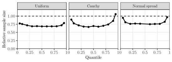
Figure 6: Average ratio of sample size for Theorem 6 to sample size for naive strategy of stopping when per-arm confidence intervals are disjoint, based on 256 simulation runs. All simulations involve sampling each of two arms in alternation and conducting a two-sided sequential test for equality of the given quantile with $\alpha=0.05$. Arm distributions are identical to those in Figure 5. Theorem 6 reduces the necessary sample size by about 25% in most cases, although the advantage diminishes for extreme quantiles, and becomes a slight disadvantage for the case of testing the 95%ile of a Cauchy distribution.

Figure 6 illustrates the performance of the two-sided test (128) relative to the naive strategy mentioned at the beginning of this section, based on simultaneously-valid confidence sequences for the mean of each arm. Across most scenarios, Theorem 6 achieves significance with about 25% fewer samples than the naive strategy. The exceptional cases involve extreme quantiles, with $p$ close to zero or one. In these cases, the minimization over $x$ in (128), which requires that all values of $x$ are implausible based on combined evidence, sometimes leads to more conservative behavior than the use of simultaneous confidence sequences, which require only the existence of some value of $x$ which is implausible for both arms.

Typically, A/B tests are run with a single control or baseline arm to be compared against multiple treatment arms (Kohavi et al., 2009). In such cases, rather than computing a $p$-value for each pairwise comparison of treatment arm to control, we may wish to compute a $p$-value for the null hypothesis that the control is no worse than any of the treatment arms. Formally, we have $K$ arms in total, arm $k=1$ is the control arm, and we wish to test the global null $H_{0}:Q_{1}(p)\geq\max_{k}Q_{k}(p)$. Note $H_{0}=\cap_{k\geq 2}H_{0k}$, where we define $H_{0k}:Q_{1}(p)\geq Q_{k}(p)$ for $k=2,\dots,K$. Using a Bonferroni correction across $k=2,\dots,K$, it follows that

$$p_{t}=(K-1)\exp\left\{-\max_{k=2,\dots,K}\min_{x\in\mathbb{R}}\left[G^{+}_{1,t}(x)+G^{-}_{k,t}(x)\right]\right\}$$ (133)

gives an always-valid $p$-value process for the global null $H_{0}$.

Any of the $p$-values obtained in this section may be used for online control of the false discovery rate in large-scale, “doubly-sequential” experimentation, when one is faced with a potentially infinite sequence of sequential experiments (Yang et al., 2017; Zrnic et al., 2021).

B.2 Sequential Kolmogorov-Smirnov tests and a test of stochastic dominance

As an easy consequence of Theorem 2, we obtain a sequential analogue of the one-sample Kolmogorov-Smirnov test. Suppose we wish to sequentially test the null hypothesis $H_{0}:F=F_{0}$ for some fixed distribution $F_{0}$. Write

$$C(A,\alpha)\coloneqq\inf\left\{c>0:\alpha_{A,c}\leq\alpha\right\},$$ (134)

where $\alpha_{A,c}$ is defined in Theorem 2.

Corollary 3.

For any $\alpha\in(0,1)$ and $A>1/\sqrt{2}$, the test which rejects $H_{0}:F=F_{0}$ as soon as $\lVert\widehat{F}_{t}-F_{0}\rVert_{\infty}>A\sqrt{t^{-1}(\log\log(et/m)+C(A,\alpha))}$ gives a valid, open-ended sequential test of $H_{0}$ with power one. That is, if $H_{0}$ is true, the probability of stopping is at most $\alpha$, while if $H_{0}$ is false, the probability of stopping is one.

The fact that this test has power one follows from the Glivenko-Cantelli theorem and the fact that the boundary becomes arbitrarily small, $A\sqrt{t^{-1}(\log\log(et/m)+C(A,\alpha))}\to 0$ as $t\to\infty$ (Robbins, 1970). A sequential two-sample test follows from an application of the triangle inequality and a union bound, by applying Theorem 2 to each sample with error probability $\alpha/2$. Here we suppose $(X_{t})_{t=1}^{\infty}$ are i.i.d. from distribution $F$, while $(Y_{t})_{t=1}^{\infty}$ are i.i.d. from distribution $G$, and we wish to test the null hypothesis $H_{0}:F=G$. We denote the empirical CDF of $Y_{1},\dots,Y_{t}$ by $\widehat{G}_{t}$.

Corollary 4.

For any $\alpha\in(0,1)$ and $A>1/\sqrt{2}$, the test which rejects $H_{0}:F=G$ as soon as $\lVert\widehat{F}_{t}-\widehat{G}_{t}\rVert_{\infty}>2A\sqrt{t^{-1}(\log\log(et/m)+C(A,\alpha/2))}$ gives a valid, open-ended sequential test of $H_{0}$ with power one.

A one-sided variant of Corollary 4 tests $H_{0}:F(x)<G(x)$ for some $x\in\mathcal{X}$ or $F(x)=G(x)$ for all $x\in\mathcal{X}$ against $H_{1}:F(x)\geq G(x)$ for all $x\in\mathcal{X}$ and $F(x)>G(x)$ for some $x\in\mathcal{X}$. This yields a sequential test of stochastic dominance.

Corollary 5.

For any $\alpha\in(0,1)$ and $A>1/\sqrt{2}$, the test which rejects $H_{0}:F\leq G$ as soon as

$$\inf_{x\in\mathcal{X}}\left[\widehat{F}_{t}(x)-\widehat{G}_{t}(x)\right]\geq 2A\sqrt{t^{-1}(\log\log(et/m)+C(A,\alpha))},\text{with strict inequality for some $x$},$$ (135)

gives a valid, open-ended sequential test of $H_{0}$ with power one.

In Corollary 5, we are able to use error probability $\alpha$ in our application of Theorem 2 to each sample, rather than $\alpha/2$. This holds because we need only a one-sided confidence bound on each CDF rather than the two-sided bound of Theorem 2. Since the proof of Theorem 2 involves a union bound over the upper and lower confidence bounds, it yields valid one-sided bounds as well, each with half the total error probability.

Appendix C Additional proofs

For reference, we present the full set of implications between $\widehat{F}_{t}$, $\widehat{F}^{-}_{t}$, $\widehat{Q}_{t}$, and $\widehat{Q}^{-}_{t}$:

$$\widehat{F}_{t}(x)>p\enskip \Rightarrow\enskip x\geq\widehat{Q}_{t}(p)$$ (136)

$$\widehat{F}_{t}(x)\geq p\enskip \Leftrightarrow\enskip x\geq\widehat{Q}^{-}_{t}(p)$$ (137)

$$\widehat{F}_{t}(x)<p\enskip \Leftrightarrow\enskip x<\widehat{Q}^{-}_{t}(p)$$ (138)

$$\widehat{F}_{t}(x)\leq p\enskip \Rightarrow\enskip x\leq\widehat{Q}_{t}(p)$$ (139)

$$\widehat{F}^{-}_{t}(x)>p\enskip \Leftrightarrow\enskip x>\widehat{Q}_{t}(p)$$ (140)

$$\widehat{F}^{-}_{t}(x)\geq p\enskip \Rightarrow\enskip x\geq\widehat{Q}^{-}_{t}(p)$$ (141)

$$\widehat{F}^{-}_{t}(x)<p\enskip \Rightarrow\enskip x\leq\widehat{Q}^{-}_{t}(p)$$ (142)

$$\widehat{F}^{-}_{t}(x)\leq p\enskip \Leftrightarrow\enskip x\leq\widehat{Q}_{t}(p).$$ (143)

C.1 Derivation of asymptotic expansion (10)

The function $\widetilde{f}_{t}(p)$ defined in (45) is an instance of ($1/t$ times) a conjugate mixture boundary (Howard et al., 2021, Section 3.2), and $M_{p,r}(s,v)$ defined in (46) is a mixture supermartingale. Mixture supermartingale have the generic form $\int\exp\left\{\lambda s-\psi(\lambda)v\right\}\mathop{}\!\mathrm{d}F(\lambda)$, and $M_{p,r}(s,v)$ is derived in Proposition 7 of Howard et al. (2021) using the function $\psi$ defined above in (40) and a Beta distribution with parameters $r/(1-p)$ and $r/p$ on the transformed parameter $x=\left[1+\frac{1-p}{p}\exp(-\lambda)\right]^{-1}$ for $F$. Proposition 2 of Howard et al. (2021) yields the generic asymptotic expansion

$$\sqrt{v\left[c\log\left(\frac{cv}{2\pi\alpha^{2}f^{2}(0)}\right)+o(1)\right]},$$ (144)

where

• $v$ is the “variance time” argument, which we are taking as $p(1-p)t$ in defining $\widetilde{f}_{t}(p)$;

• $c=\psi^{\prime\prime}(0_{+})=1$; and

• $f(0)=p(1-p)f_{\beta}\left(p;\frac{r}{1-p},\frac{r}{p}\right)$ is the density of the mixture distribution on $\lambda$, which is a transformed Beta distribution as noted above, at $\lambda=0$.

Comparing (144) with (10), we see that

$$C_{p,r}=\sqrt{2\pi}f(0)=\sqrt{2\pi}p(1-p)f_{\beta}\left(p;\frac{r}{1-p},\frac{r}{p}\right).$$ (145)

Note that as $p\downarrow 0$ or $p\uparrow 1$,

$$C_{p,r}\sim\frac{\sqrt{2\pi}r^{r}}{e^{r}\Gamma(r)},$$ (146)

so that $C_{p,r}$ approaches a constant as $p\downarrow 0$ or $p\uparrow 1$. By Stirling’s formula, this latter expression is asymptotic to $\sqrt{r}$ as $r\uparrow\infty$.

C.2 Proof of Proposition 1

The classical law of the iterated logarithm implies

$$\limsup_{t\to\infty}\frac{\widehat{F}_{t}(Q(p))-p}{\sqrt{t^{-1}\log\log t}}=\sqrt{2p(1-p)},\,\text{a.s.}$$ (147)

Since $\liminf_{t\to\infty}\sqrt{t^{-1}\log\log t}/u_{t}>1/\sqrt{2p(1-p)}$, we have

$$\limsup_{t\to\infty}\frac{\widehat{F}_{t}(Q(p))-p}{u_{t}}\geq\left(\limsup_{t\to\infty}\frac{\widehat{F}_{t}(Q(p))-p}{\sqrt{t^{-1}\log\log t}}\right)\left(\liminf_{t\to\infty}\frac{\sqrt{t^{-1}\log\log t}}{u_{t}}\right)>1,\,\text{a.s.}$$ (148)

Hence, with probability one, there exists $t_{0}$ such that $\widehat{F}_{t_{0}}(Q(p))>p+u_{t_{0}}$. Then property (136) implies $Q(p)\geq\widehat{Q}_{t_{0}}(p+u_{t_{0}})$, which yields the desired conclusion. ∎

C.3 Proof of Corollary 1

Fix any $\epsilon>0$ and let $A_{\epsilon}=1/\sqrt{2}+\epsilon$. Applying Theorem 2 with $m=1$ and any $C>0$, the second result (52) implies

$$\limsup_{t\to\infty}\frac{\lVert\widehat{F}_{t}-F\rVert_{\infty}}{A_{\epsilon}\sqrt{t^{-1}(\log\log(et)+C)}}=\limsup_{t\to\infty}\frac{\lVert\widehat{F}_{t}-F\rVert_{\infty}}{A_{\epsilon}\sqrt{t^{-1}\log\log t}}\leq 1\text{ almost surely}.$$ (149)

The conclusion follows since $\epsilon$ was arbitrary.

C.4 Proof of Corollary 2

Theorem 2 implies that $\widehat{F}_{t}(Q^{-}(p))\geq F(Q^{-}(p))-g_{t}$ uniformly over $t\geq m$ and $p\in(0,1)$ with high probability. Hence (137) implies $Q^{-}(p)\geq\widehat{Q}^{-}_{t}(F(Q^{-}(p))-g_{t})\geq\widehat{Q}^{-}_{t}(p-g_{t})$. Likewise, Theorem 2 implies $\widehat{F}_{t}(x)\leq F(x)+g_{t}$ uniformly over $t\geq m$ and $x\in\mathcal{X}$ with high probability, and taking limits from the left, we also have $\widehat{F}^{-}_{t}(x)\leq F^{-}(x)+g_{t}$. Hence $\widehat{F}^{-}_{t}(Q(p))\leq F^{-}(Q(p))+g_{t}$, and (143) implies $Q(p)\leq\widehat{Q}_{t}(F^{-}(Q(p))+g_{t})\leq\widehat{Q}_{t}(p+g_{t})$. ∎

C.5 Proof of Theorem 6

We extend the definition of $S_{t}(p)$ from (38) to the two-armed setup: for $k\in\{1,2\}$, let

$$\pi_{k}(p)\coloneqq\begin{cases}0,&F_{k}(Q_{k}(p))=F_{k}^{-}(Q_{k}(p)),\\ \frac{p-F_{k}^{-}(Q_{k}(p))}{F_{k}(Q_{k}(p))-F^{-}(Q_{k}(p))},&F_{k}(Q_{k}(p))>F_{k}^{-}(Q_{k}(p)),\end{cases}$$ (150)

and define $S_{k,0}(p)=0$ and, for $t\in\mathbb{N}$,

$$S_{k,t}(p)\coloneqq\sum_{i=1}^{N_{k,t}}\left[1_{X_{k,i}<Q_{k}(p)}+\pi_{k}(p)1_{X_{k,i}=Q_{k}(p)}-p\right].$$ (151)

The increments are mean-zero and bounded in $[-p,1-p]$ conditional on the past, so the process $(S_{k,t}(p))$ is sub-Bernoulli with variance process $p(1-p)t$ and scale parameters $g=p,h=1-p$ (Howard et al., 2020, Fact 1(b)). Then the proof of Propositions 6 and 7 of Howard et al. (2021) shows that the processes

$$L_{k,t} \coloneqq M_{p,r}(S_{k,t}(p),p(1-p)N_{k,t}),$$ (152)

$$L^{+}_{k,t} \coloneqq M^{1}_{p,r}(S_{k,t}(p),p(1-p)N_{k,t}),\quad\text{and}$$ (153)

$$L^{-}_{k,t} \coloneqq M^{1}_{1-p,r}(-S_{k,t}(p),p(1-p)N_{k,t})$$ (154)

are nonnegative supermartingales with $\mathbb{E}L_{k,0}=\mathbb{E}L^{+}_{k,0}=\mathbb{E}L^{-}_{k,0}=1$, with respect to the filtration $(\mathcal{F}_{t})$ generated by the observations.

For the two-sided test, we form the product $\widetilde{L}_{t}\coloneqq L_{1,t}L_{2,t}$, which is also a nonnegative supermartingale. Indeed, if we choose to sample arm 1 at time $t$, a choice which is predictable with respect to $(\mathcal{F}_{t})$, then $L_{2,t}=L_{2,t-1}$, so $\mathbb{E}\left(\left.\widetilde{L}_{t}\,\right|\,\mathcal{F}_{t-1}\right)=L_{2,t-1}\mathbb{E}\left(\left.L_{1,t}\,\right|\,\mathcal{F}_{t-1}\right)\leq\widetilde{L}_{t-1}$; likewise if we choose to sample arm 2. Then Ville’s inequality yields

$$\mathbb{P}\left(\exists t\in\mathbb{N}:\widetilde{L}_{t}\geq\frac{1}{\alpha}\right)\leq\alpha.$$ (155)

Our goal is to lower bound $\widetilde{L}_{t}$ under the null hypothesis $H_{0}:Q_{2}(p)-Q_{1}(p)=\delta_{\star}$. Suppose we strengthen this hypothesis to $Q_{1}(p)=x_{1}$ and $Q_{2}(p)=x_{2}\coloneqq x_{1}+\delta_{\star}$ for some $x_{1}\in\mathbb{R}$. We still cannot compute $S_{k,t}(p)$ without knowledge of $\pi_{k}(p)$. But since $\pi_{k}(p)\in[0,1]$, we are assured $S_{k,t}(p)/N_{k,t}\in\mathcal{D}_{k,t}(x_{k})$ for all $t$, so that $\log L_{k,t}\geq G_{k,t}(x_{k})$ for $k=1,2$, by the definitions of $L_{k,t}$ and $G_{k,t}$. Hence, on the stronger hypothesis, we have

$$\log\widetilde{L}_{t}\geq G_{1,t}(x_{1})+G_{2,t}(x_{1}+\delta_{\star}),\quad\text{for all $t\in\mathbb{N}$}.$$ (156)

On $H_{0}$, then, we have

$$\log\widetilde{L}_{t}\geq\min_{x\in\mathbb{R}}\left[G_{1,t}(x)+G_{2,t}(x+\delta_{\star})\right]\quad\text{for all $t\in\mathbb{N}$},$$ (157)

and the conclusion (128) for the two-sided test follows from (155) and (157).

For the one-sided test, we follow a similar argument. Form the product $\widetilde{L}^{1}_{t}\coloneqq L_{1,t}^{+}L_{2,t}^{-}$, which is a supermartingale by an analogous argument as that above for $\widetilde{L}_{t}$. Ville’s inequality yields $\mathbb{P}\left(\exists t\in\mathbb{N}:\widetilde{L}^{1}_{t}\geq 1/\alpha\right)\leq\alpha$. Now since $M^{1}_{p,r}(\cdot,v)$ is nondecreasing (Howard et al., 2021, Appendix C and proof of Proposition 7), $G^{+}_{k,t}$ is nondecreasing while $G^{-}_{k,t}$ is nonincreasing, which implies

$$G^{+}_{k,t}(x) =\min_{a\in\mathcal{D}_{k,t}(x)}\log M^{1}_{p,r}\left((a-p)N_{k,t},p(1-p)N_{k,t}\right),$$ (158)

$$G^{-}_{k,t}(x) =\min_{a\in\mathcal{D}_{k,t}(x)}\log M^{1}_{1-p,r}\left(-(a-p)N_{k,t},p(1-p)N_{k,t}\right).$$ (159)

Suppose we strengthen the null hypothesis to $Q_{1}(p)=x_{1}$ and $Q_{2}(p)=x_{2}\leq x_{1}+\delta_{\star}$ for some $x_{1},x_{2}\in\mathbb{R}$. Then the argument above shows that $\log L^{\pm}_{k,t}\geq G^{\pm}_{k,t}(x_{k})$ for $k=1,2$, so that

$$\log\widetilde{L}^{1}_{t} \geq G^{+}_{1,t}(x_{1})+G^{-}_{2,t}(x_{2})$$ (160)

$$\geq G^{+}_{1,t}(x_{1})+G^{-}_{2,t}(x_{1}+\delta_{\star}),$$ (161)

since $x_{2}\leq x_{1}+\delta_{\star}$ and $G^{-}_{2,t}$ is nonincreasing. On $H_{0}:Q_{2}(p)-Q_{1}(p)\leq\delta_{\star}$, then, we have

$$\log\widetilde{L}^{1}_{t}\geq\min_{x\in\mathbb{R}}\left[G^{+}_{1,t}(x)+G^{-}_{2,t}(x+\delta_{\star})\right]\quad\text{for all $t\in\mathbb{N}$},$$ (162)

and the conclusion (129) for the one-sided test follows as before. ∎

Appendix D Details of Figure 2

Here we give details for each of the bounds presented in Figure 2. Additionally, Figure 7 includes all bounds together in a single plot, along with two more bounds: the DKW bounds which is uniform over quantiles for a fixed time, and the pointwise Bernoulli bound which is valid for a fixed quantile at a fixed time. In all cases, we use a two-sided error probability of 0.05, and all bounds are tuned for a minimum sample size of $m=32$.

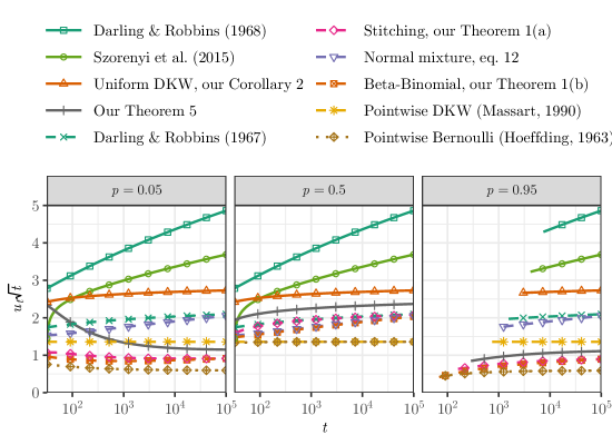
Figure 7: Plot of upper confidence bound radii $u_{t}$, normalized by $\sqrt{t}$ to facilitate comparison. Each panel shows estimation radius for a different quantile, $p=0.05$, 0.5, and 0.95, respectively. All bounds correspond to two-sided $\alpha=0.05$. Dotted line is valid for a fixed quantile at a fixed time, dashed lines are valid uniformly over either time or quantiles, and solid lines are valid uniformly over both time and quantiles. In right panel, lines start at the sample size for which the upper confidence bound becomes nontrivial. See Appendix D for details of each bound shown.

• Darling and Robbins (1968, Theorem 4) give a test based on a bound for $\lVert\widehat{F}_{t}-F\rVert_{\infty}$ which achieves uniformity over time via a union bound over $t\geq m$. We follow their guidance in remark (d), p. 808 to choose $u_{t}=\sqrt{t^{-2}(t+1)(2\log t+0.601)}$.

• Szörényi et al. (2015, Proposition 1) uses a similar union-bounding argument on the optimal DKW inequality of Massart (1990). We adjust their result so that the union bound only applies over $t\geq 32$, yielding $u_{t}=\sqrt{t^{-1}(\log(t-31)+2.093)}$.

• For Corollary 2, we set $A=0.85$ and numerically choose $C=8.123$, so $u_{t}=0.85\sqrt{t^{-1}(\log\log(et/32)+8.123)}$.

• For Theorem 5, we set $\delta=0.5$, $\eta=2.041$, and $s=1.4$.

• Darling and Robbins (1967a, Section 2) give an explicit confidence sequence for the median, which applies to other quantiles as well. In this case,

  $$u_{t}=(3/2\sqrt{2})\sqrt{t^{-1}(\log\log t+1.457)}.$$ (163)

• For Theorem 1(a), we set $\eta=2.04$ and $s=1.4$, as in (9).

• For Theorem 1(b), we set $r=0.145$ for $p=0.05$ and $p=0.95$, while $r=0.758$ for $p=0.5$, in accordance with (21).

• The normal mixture bound (12) uses $r=0.504$.

• The DKW bound for a fixed time uses $u_{t}=1.358\sqrt{n}$.

• The fixed-sample Bernoulli bound is based on Hoeffding (1963, equation 2.1), and is given by the solution in $x$ to $t\,\text{KL}\left(\left.p+x\,\right\rVert\,p\right)=\log(2/0.05)$, where

  $$\text{KL}\left(\left.q\,\right\rVert\,p\right)=q\log\left(\frac{q}{p}\right)+(1-q)\log\left(\frac{1-q}{1-p}\right)$$ (164)

  denotes the Bernoulli Kullback-Leibler divergence.

Appendix E Implementation details for Theorem 6

The tests in Theorem 6 involve minimizing over possibly multimodal sums of the functions $G_{k,t}(x)$, $G^{+}_{k,t}(x)$, and $G^{-}_{k,t}(x)$, with $G_{k,t}$ itself defined in terms of a minimization. In this section, we discuss details for implementing these tests, which require $\mathcal{O}(t\log t)$ time in the worst case. We focus the discussion on the two-sided test (128). The one-sided test (129) is similar, as we briefly discuss at the end of the section.

Fix any $p\in(0,1)$, and $r>0$. The key observation is that $\log M_{p,r}(s,p(1-p)n)$ is continuous and unimodal on the domain $s\in[-pn,(1-p)n]$ for any $n\in\mathbb{N}$, since $M_{p,r}(s,v)$ is convex and finite on the domain $s\in[-v/(1-p),v/p]$ (Howard et al., 2021, Appendix C). (It may be verified that $\log M_{p,r}(\cdot,v)$ is itself convex, but we do not use that fact here.) Let

$$a_{k,t}=\operatorname*{arg\,min}_{a\in[0,1]}\log M_{p,r}((a-p)N_{k,t},p(1-p)N_{k,t}),$$ (165)

which may be found via numerical optimization. Then from the definition of $G_{k,t}(x)$ and its unimodality, together with (138) and (140), we have

$$G_{k,t}(x)=\begin{cases}\log M_{p,r}\big{(}(\widehat{F}_{k,t}(x)-p)N_{k,t},\,p(1-p)N_{k,t}\big{)},&x<\widehat{Q}^{-}_{k,t}\left(a_{k,t}\right),\\ \log M_{p,r}\big{(}(a_{\star}-p)N_{k,t},\,p(1-p)N_{k,t}\big{)},&\widehat{Q}^{-}_{k,t}\left(a_{k,t}\right)\leq x\leq\widehat{Q}_{k,t}\left(a_{k,t}\right),\\ \log M_{p,r}\big{(}(\widehat{F}^{-}_{k,t}(x)-p)N_{k,t},\,p(1-p)N_{k,t}\big{)},&x>\widehat{Q}_{k,t}\left(a_{k,t}\right).\end{cases}$$ (166)

So once the value $a_{k,t}$ has been found, $G_{k,t}(x)$ is given in closed form for any $x$. Note also that $G_{k,t}(x)$ is nonincreasing on $x<\widehat{Q}^{-}_{k,t}(a_{k,t})$, nondecreasing on $x>\widehat{Q}_{k,t}(a_{k,t})$, and constant on $\widehat{Q}^{-}_{k,t}(a_{k,t})\leq x\leq\widehat{Q}_{k,t}(a_{k,t})$.

Unfortunately, the objective $l(x)\coloneqq G_{1,t}(x)+G_{2,t}(x+\delta^{\star})$ is not unimodal in general. Suppose without loss of generality that $\widehat{Q}_{1,t}(a_{1,t})\leq\widehat{Q}_{2,t}(a_{2,t})-\delta^{\star}$, so that $G_{1,t}(x)$ begins increasing before $G_{2,t}(x+\delta^{\star})$ does, and define $x_{-}\coloneqq\widehat{Q}_{1,t}(a_{1,t})$ and $x_{+}\coloneqq\widehat{Q}^{-}_{2,t}(a_{2,t})-\delta^{\star}$. Then $l(x)$ is nonincreasing on $x<x_{-}$ and nondecreasing on $x>x_{+}$, but in general may achieve many local minima on $[x_{-},x_{+}]$. On this interval, $l(x)$ only decreases at values $x=X_{2,s}+\delta^{\star}$ for some $s\leq t$, i.e., $l(x)$ decreases at values of $x$ which have been observed from the second arm. So to find the minimum, we must evaluate $l(x)$ at each point $x\in\{x_{-},x_{+}\}\cup\{X_{2,s}+\delta^{\star}:s\leq t,x_{-}\leq X_{2,s}+\delta^{\star}\leq x_{+}\}$. This requires $\mathcal{O}(N_{2,t})$ time in general, though the use of $x_{-}$ and $x_{+}$ will improve constants. In the corner case $x_{+}\leq x_{-}$, we must have $l(x)$ achieving its minimum at $x=x_{-}$.

We also need to efficiently evaluate the empirical CDFs $\widehat{F}_{k,t}$ and $\widehat{F}^{-}_{k,t}$ and the empirical quantile functions $\widehat{Q}_{k,t}$, and $\widehat{Q}^{-}_{k,t}$. For this, we use a balanced binary tree in which each node is augmented with the size of the subtree rooted at that node. This allows evaluation of the empirical CDFs and quantile functions in $\mathcal{O}(\log N_{k,t})$ time.

For the one-sided test (129), we have that $G^{+}_{k,t}(x)$ is nondecreasing and $G^{-}_{k,t}(x)$ is nonincreasing over all $x\in\mathcal{X}$, since $M^{1}_{p,r}(s,v)$ is nondecreasing (Howard et al., 2021, Appendix C). We must therefore search over all values $x\in\{X_{2,s}+\delta^{\star}:s\leq t\}$.

Appendix F Full comparison of quantile best-arm strategies

Figure 8 adds to Figure 5 two additional best-arm strategies. First, we include a variant of Algorithm 1 from Szörényi et al. (2015), “QPAC”, in which we simply replace their confidence sequence with our tighter confidence sequence based on a one-sided variant of the beta-binomial confidence sequence Theorem 1(b). This shows the improvement due to our confidence sequence alone under the QPAC sampling strategy. Second, we include our QLUCB algorithm with the same confidence sequence as in Szörényi et al. (2015). Comparing this to the original algorithm of Szörényi et al. (2015) shows the improvement due to our sampling strategy alone. The plot shows that both the confidence sequence and the sampling strategy lead to improvements, but the confidence sequence contributes more to the overall improvement.

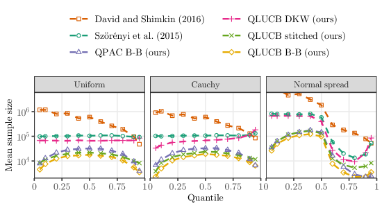
Figure 8: Average sample size for various quantile best-arm identification algorithms based on 64 simulation runs, with $\epsilon=0.025$ and $\pi=0.05,0.1,0.2,\dots,0.8,0.9,0.95$. Left panel shows results for arms with uniform distributions on intervals of length one; middle panel shows arms with Cauchy distributions have unit scale; and right panel shows arms with standard normal distributions except for one, which has a standard deviation of two instead of one. In this last case, the exceptional arm is best for quantiles above $0.53$, while for quantiles below $0.45$, the other arms are all $\epsilon$-optimal. Plot includes Algorithm 2 of David and Shimkin (2016), Algorithm 1 of Szörényi et al. (2015), and a modification of Algorithm 1 of Szörényi et al. (2015), “QPAC B-B”, which uses the one-sided variant of our beta-binomial confidence sequence Theorem 1(b). We compare our QLUCB algorithm based on three different confidence sequences: the stitched confidence sequence (24) based on Theorem 1(a); a one-sided variant of the beta-binomial (“B-B”) confidence sequence, Theorem 1(b); and the same DKW-plus-union-bound confidence sequence as QPAC, for comparison. Observe that our proposed changes in algorithm and in confidence sequences both yield improvements, separately and together.

Appendix G Analogy to multiple testing

From a multiple testing point of view, one may view our confidence sequences as controlling a familywise error rate for miscoverage: with high probability, all constructed intervals will simultaneously achieve coverage. An alternative goal would be to control the false coverage rate, the expected proportion of intervals that fail to cover their parameters. Here we observe that this goal is achieved, asymptotically, by any asymptotically pointwise-valid intervals:

Proposition 2.

Suppose the sequence of $(1-\alpha)$-confidence intervals $(\text{CI}_{t})_{t=1}^{\infty}$ is asymptotically pointwise valid:

$$\limsup_{t\to\infty}\mathbb{P}(\text{CI}_{t}\text{ fails to cover})\leq\alpha.$$ (167)

Then the sequence achieves asymptotic false coverage rate control:

$$\limsup_{t\to\infty}\mathbb{E}\left[\frac{1}{t}\sum_{i=1}^{t}1\{\text{CI}_{i}\text{ fails to cover}\}\right]\leq\alpha.$$ (168)

Proof.

Write $p_{t}\coloneqq\mathbb{P}(\text{CI}_{t}\text{ fails to cover})$. By assumption $\limsup_{t\to\infty}p_{t}\leq\alpha$, and by linearity of expectation, the limit in (168) is $\limsup_{t\to\infty}t^{-1}\sum_{i=1}^{t}p_{i}$. For any $\epsilon>0$, choose $s$ sufficiently large that $p_{t}\leq\alpha+\epsilon$ for all $t>s$. Then

$$\limsup_{t\to\infty}\frac{1}{t}\sum_{i=1}^{t}p_{i}\leq\limsup_{t\to\infty}\frac{1}{t}\sum_{i=1}^{s}p_{i}+\limsup_{t\to\infty}\frac{1}{t}\sum_{i=s+1}^{t}p_{i}=\limsup_{t\to\infty}\frac{1}{t}\sum_{i=s+1}^{t}p_{i}\leq\alpha+\epsilon,$$ (169)

by our choice of $s$. As $\epsilon$ was arbitrary, the proof is complete. ∎

Thus for asymptotic FCR-controlled confidence intervals for a quantile, we need only compute asymptotically pointwise-valid confidence intervals for quantile, and these follow generically from the central limit theorem. Let $z_{p}$ denote the $p$-quantile of a standard normal distribution.

Proposition 3.

In the setting of Section 3, for any $p\in(0,1)$ and any $\alpha\in(0,1)$, we have

$$\lim_{t\to\infty}\mathbb{P}\Bigg{(}Q^{-}(p)<\widehat{Q}_{t}\left(p-z_{1-\alpha/2}\sqrt{\frac{p(1-p)}{t}}\right)\\ \text{ or }Q(p)>\widehat{Q}^{-}_{t}\left(p+z_{1-\alpha/2}\sqrt{\frac{p(1-p)}{t}}\right)\Bigg{)}\leq\alpha.$$ (170)

Proof.

Define $S_{t}\coloneqq S_{t}(p)$ from (38), a sum of i.i.d., mean-zero, bounded increments $\Delta S_{t}\coloneqq S_{t}-S_{t-1}\in[-p,1-p]$ (taking $\Delta S_{1}=S_{1}$). The variance $\mathbb{E}S_{1}^{2}$ is upper bounded by $p(1-p)$; indeed, $0\geq\mathbb{E}(\Delta S_{1}+p)(\Delta S_{1}-(1-p))=\mathbb{E}\Delta S_{1}^{2}-p(1-p)$. By the central limit theorem,

$$\lim_{t\to\infty}\mathbb{P}\left(\left\lvert S_{t}\right\rvert\geq z_{1-\alpha/2}\sqrt{\frac{p(1-p)}{t}}\right)\leq\lim_{t\to\infty}\mathbb{P}\left(\left\lvert S_{t}\right\rvert\geq z_{1-\alpha/2}\sqrt{t\mathbb{E}\Delta S_{1}^{2}}\right)=\alpha.$$ (171)

Now repeat the argument behind (44), (48), and (49) to conclude (170). ∎

References

- (1)
- Anderson (1984) Anderson, C. W. (1984), Large Deviations of Extremes, in J. T. de Oliveira, ed., ‘Statistical Extremes and Applications’, Springer Netherlands, Dordrecht, pp. 325–340.
- Arnold et al. (2008) Arnold, B. C., Balakrishnan, N. and Nagaraja, H. N. (2008), A First Course in Order Statistics, Society for Industrial and Applied Mathematics.
- Boucheron et al. (2013) Boucheron, S., Lugosi, G. and Massart, P. (2013), Concentration inequalities: a nonasymptotic theory of independence, 1st edn, Oxford University Press, Oxford.
- Boucheron and Thomas (2012) Boucheron, S. and Thomas, M. (2012), ‘Concentration inequalities for order statistics’, Electronic Communications in Probability 17, 1–12.
- Bubeck et al. (2009) Bubeck, S., Munos, R. and Stoltz, G. (2009), Pure exploration in multi-armed bandits problems, in ‘International Conference on Algorithmic Learning Theory’, Springer, pp. 23–37.
- Corless et al. (1996) Corless, R. M., Gonnet, G. H., Hare, D. E. G., Jeffrey, D. J. and Knuth, D. E. (1996), ‘On the Lambert W function’, Advances in Computational Mathematics 5(1), 329–359.