Ranking Policy Gradient

Abstract

Sample inefficiency is a long-lasting problem in reinforcement learning (RL). The state-of-the-art estimates the optimal action values while it usually involves an extensive search over the state-action space and unstable optimization. Towards the sample-efficient RL, we propose ranking policy gradient (RPG), a policy gradient method that learns the optimal rank of a set of discrete actions. To accelerate the learning of policy gradient methods, we establish the equivalence between maximizing the lower bound of return and imitating a near-optimal policy without accessing any oracles. These results lead to a general off-policy learning framework, which preserves the optimality, reduces variance, and improves the sample-efficiency. Furthermore, the sample complexity of RPG does not depend on the dimension of state space, which enables RPG for large-scale problems. We conduct extensive experiments showing that when consolidating with the off-policy learning framework, RPG substantially reduces the sample complexity, comparing to the state-of-the-art.

Keywords: sample-efficiency, off-policy learning, learning to rank, policy gradient, deep reinforcement learning.

1 Introduction

One of the major challenges in reinforcement learning (RL) is the high sample complexity (Kakade et al., 2003), which is the number of samples must be collected to conduct successful learning. There are different reasons leading to poor sample efficiency of RL (Yu, 2018). Because policy gradient algorithms directly optimizing return estimated from rollouts (e.g., Reinforce (Williams, 1992)) could suffer from high variance (Sutton and Barto, 2018), value function baselines were introduced by actor-critic methods to reduce the variance and improve the sample-efficiency. However, since a value function is associated with a certain policy, the samples collected by former policies cannot be readily used without complicated manipulations (Degris et al., 2012) and extensive parameter tuning (Nachum et al., 2017). Such an on-policy requirement increases the difficulty of sample-efficient learning.

On the other hand, off-policy methods, such as one-step $Q$-learning (Watkins and Dayan, 1992) and variants of deep $Q$ networks (DQN) (Mnih et al., 2015; Hessel et al., 2017; Dabney et al., 2018; Van Hasselt et al., 2016; Schaul et al., 2015), enjoys the advantage of learning from any trajectory sampled from the same environment (i.e., off-policy learning), are currently among the most sample-efficient algorithms. These algorithms, however, often require extensive searching (Bertsekas and Tsitsiklis, 1996, Chap. 5) over the large state-action space to estimate the optimal action value function. Another deficiency is that, the combination of off-policy learning, bootstrapping, and function approximation, making up what Sutton and Barto (2018) called the "deadly triad", can easily lead to unstable or even divergent learning (Sutton and Barto, 2018, Chap. 11). These inherent issues limit their sample-efficiency.

Towards addressing the aforementioned challenge, we approach the sample-efficient reinforcement learning from a ranking perspective. Instead of estimating optimal action value function, we concentrate on learning optimal rank of actions. The rank of actions depends on the relative action values. As long as the relative action values preserve the same rank of actions as the optimal action values ($Q$-values), we choose the same optimal action. To learn optimal relative action values, we propose the ranking policy gradient (RPG) that optimizes the actions’ rank with respect to the long-term reward by learning the pairwise relationship among actions.

Ranking Policy Gradient (RPG) that directly optimizes relative action values to maximize the return is a policy gradient method. The track of off-policy actor-critic methods (Degris et al., 2012; Gu et al., 2016; Wang et al., 2016) have made substantial progress on improving the sample-efficiency of policy gradient. However, the fundamental difficulty of learning stability associated with the bias-variance trade-off remains (Nachum et al., 2017). In this work, we first exploit the equivalence between RL optimizing the lower bound of return and supervised learning that imitates a specific optimal policy. Build upon this theoretical foundation, we propose a general off-policy learning framework that equips the generalized policy iteration (Sutton and Barto, 2018, Chap. 4) with an external step of supervised learning. The proposed off-policy learning not only enjoys the property of optimality preserving (unbiasedness), but also largely reduces the variance of policy gradient because of its independence of the horizon and reward scale. Furthermore, this learning paradigm leads to a sample complexity analysis of large-scale MDP, in a non-tabular setting without the linear dependence on the state space. Based on our sample-complexity analysis, we define the exploration efficiency that quantitatively evaluates different exploration methods. Besides, we empirically show that there is a trade-off between optimality and sample-efficiency, which is well aligned with our theoretical indication. Last but not least, we demonstrate that the proposed approach, consolidating the RPG with off-policy learning, significantly outperforms the state-of-the-art (Hessel et al., 2017; Bellemare et al., 2017; Dabney et al., 2018; Mnih et al., 2015).

2 Related works

Sample Efficiency. The sample efficient reinforcement learning can be roughly divided into two categories. The first category includes variants of $Q$-learning (Mnih et al., 2015; Schaul et al., 2015; Van Hasselt et al., 2016; Hessel et al., 2017). The main advantage of $Q$-learning methods is the use of off-policy learning, which is essential towards sample efficiency. The representative DQN (Mnih et al., 2015) introduced deep neural network in $Q$-learning, which further inspried a track of successful DQN variants such as Double DQN (Van Hasselt et al., 2016), Dueling networks (Wang et al., 2015), prioritized experience replay (Schaul et al., 2015), and Rainbow (Hessel et al., 2017). The second category is the actor-critic approaches. Most of recent works (Degris et al., 2012; Wang et al., 2016; Gruslys et al., 2018) in this category leveraged importance sampling by re-weighting the samples to correct the estimation bias and reduce variance. The main advantage is in the wall-clock times due to the distributed framework, firstly presented in (Mnih et al., 2016), instead of the sample-efficiency. As of the time of writing, the variants of DQN (Hessel et al., 2017; Dabney et al., 2018; Bellemare et al., 2017; Schaul et al., 2015; Van Hasselt et al., 2016) are among the algorithms of most sample efficiency, which are adopted as our baselines for comparison.

RL as Supervised Learning. Many efforts have focused on developing the connections between RL and supervised learning, such as Expectation-Maximization algorithms (Dayan and Hinton, 1997; Peters and Schaal, 2007; Kober and Peters, 2009; Abdolmaleki et al., 2018), Entropy-Regularized RL (Oh et al., 2018; Haarnoja et al., 2018), and Interactive Imitation Learning (IIL) (Daumé et al., 2009; Syed and Schapire, 2010; Ross and Bagnell, 2010; Ross et al., 2011; Sun et al., 2017; Hester et al., 2018; Osa et al., 2018). EM-based approaches apply the probabilistic framework to formulate the RL problem maximizing a lower bound of the return as a re-weighted regression problem, while it requires on-policy estimation on the expectation step. Entropy-Regularized RL optimizing entropy augmented objectives can lead to off-policy learning without the usage of importance sampling while it converges to soft optimality (Haarnoja et al., 2018).

Of the three tracks in prior works, the IIL is most closely related to our work. The IIL works firstly pointed out the connection between imitation learning and reinforcement learning (Ross and Bagnell, 2010; Syed and Schapire, 2010; Ross et al., 2011) and explore the idea of facilitating reinforcement learning by imitating experts. However, most of imitation learning algorithms assume the access to the expert policy or demonstrations. The off-policy learning framework proposed in this paper can be interpreted as an online imitation learning approach that constructs expert demonstrations during the exploration without soliciting experts, and conducts supervised learning to maximize return at the same time. In short, our approach is different from prior arts in terms of at least one of the following aspects: objectives, oracle assumptions, the optimality of learned policy, and on-policy requirement. More concretely, the proposed method is able to learn optimal policy in terms of long-term reward, without access to the oracle (such as expert policy or expert demonstration) and it can be trained both empirically and theoretically in an off-policy fashion. A more detailed discussion of the related work on reducing RL to supervised learning is provided in Appendix A.

PAC Analysis of RL. Most existing studies on sample complexity analysis (Kakade et al., 2003; Strehl et al., 2006; Kearns et al., 2000; Strehl et al., 2009; Krishnamurthy et al., 2016; Jiang et al., 2017; Jiang and Agarwal, 2018; Zanette and Brunskill, 2019) are established on the value function estimation. The proposed approach leverages the probably approximately correct framework (Valiant, 1984) in a different way such that it does not rely on the value function. Such independence directly leads to a practically sample-efficient algorithm for large-scale MDP, as we demonstrated in the experiments.

3 Notations and Problem Setting

In this paper, we consider a finite horizon $T$, discrete time Markov Decision Process (MDP) with a finite discrete state space ${\mathcal{S}}$ and for each state $s\in{\mathcal{S}}$, the action space ${\mathcal{A}}_{s}$ is finite. The environment dynamics is denoted as ${\mathbf{P}}=\{p(s^{\prime}|s,a),\forall s,s^{\prime}\in{\mathcal{S}},a\in{\mathcal{A}}_{s}\}$. We note that the dimension of action space can vary given different states. We use $m=\max_{s}\|{\mathcal{A}}_{s}\|$ to denote the maximal action dimension among all possible states. Our goal is to maximize the expected sum of positive rewards, or return $J(\theta)={\mathbf{E}}_{\tau,\pi_{\theta}}[\sum_{t=1}^{T}r(s_{t},a_{t})]$, where $0<r(s,a)<\infty,\forall s,a$. In this case, the optimal deterministic Markovian policy always exists (Puterman, 2014)[Proposition 4.4.3]. The upper bound of trajectory reward ($r(\tau)$) is denoted as $R_{\max}=\max_{\tau}r(\tau)$. A comprehensive list of notations is elaborated in Table 1.

Notations	Definition
$\lambda_{ij}$	The discrepancy of the relative action value of action $i$ and action $j$. $\lambda_{ij}=\lambda_{i}-\lambda_{j}$, where $\lambda_{i}=\lambda(s,a_{i}).$ Notice that the value here is not the estimation of return, it represents which action will have relatively higher return if followed.
$Q^{\pi}(s,a)$	The action value function or equivalently the estimation of return taking action $a$ at state $s$, following policy $\pi$.
$p_{ij}$	$p_{ij}=P(\lambda_{i}>\lambda_{j})$ denotes the probability that $i$-th action is to be ranked higher than $j$-th action. Notice that $p_{ij}$ is controlled by $\theta$ through $\lambda_{i},\lambda_{j}$
$\tau$	A trajectory $\tau=\{s(\tau,t),a(\tau,t)\}_{t=1}^{T}$ collected from the environment. It is worth noting that this trajectory is not associated with any policy. It only represents a series of state-action pairs. We also use the abbreviation $s_{t}=s(\tau,t)$, $a_{t}=a(\tau,t)$.
$r(\tau)$	The trajectory reward $r(\tau)=\sum_{t=1}^{T}r(s_{t},a_{t})$ is the sum of reward along one trajectory.
$R_{\max}$	$R_{\max}$ is the maximal possible trajectory reward, i.e., $R_{\max}=\max_{\tau}r(\tau)$. Since we focus on MDPs with finite horizon and immediate reward, therefore the trajectory reward is bounded.
$\sum_{\tau}$	The summation over all possible trajectories $\tau$.
$p(\tau)$	The probability of a specific trajectory is collected from the environment given policy $\pi_{\theta}$. $p_{\theta}(\tau)=p(s_{0})\Pi_{t=1}^{T}\pi_{\theta}(a_{t}|s_{t})p(s_{t+1}|s_{t},a_{t})$
${\mathcal{T}}$	The set of all possible near-optimal trajectories. $|{\mathcal{T}}|$ denotes the number of near-optimal trajectories in ${\mathcal{T}}$.
$n$	The number of training samples or equivalently state action pairs sampled from uniformly (near)-optimal policy.
$m$	The number of discrete actions.

Table 1: Notations

4 Ranking Policy Gradient

Value function estimation is widely used in advanced RL algorithms (Mnih et al., 2015, 2016; Schulman et al., 2017; Gruslys et al., 2018; Hessel et al., 2017; Dabney et al., 2018) to facilitate the learning process. In practice, the on-policy requirement of value function estimations in actor-critic methods has largely increased the difficulty of sample-efficient learning (Degris et al., 2012; Gruslys et al., 2018). With the advantage of off-policy learning, the DQN (Mnih et al., 2015) variants are currently among the most sample-efficient algorithms (Hessel et al., 2017; Dabney et al., 2018; Bellemare et al., 2017). For complicated tasks, the value function can align with the relative relationship of action’s return, but the absolute values are hardly accurate (Mnih et al., 2015; Ilyas et al., 2018).

The above observations motivate us to look at the decision phase of RL from a different prospect: Given a state, the decision making is to perform a relative comparison over available actions and then choose the best action, which can lead to relatively higher return than others. Therefore, an alternative solution is to learn the optimal rank of the actions, instead of deriving policy from the action values. In this section, we show how to optimize the rank of actions to maximize the return, and thus avoid the necessity of accurate estimation for optimal action value function. To learn the rank of actions, we focus on learning relative action value ($\lambda$-values), defined as follows:

Definition 1 (Relative action value ($\lambda$-values))

For a state $s$, the relative action values of $m$ actions ($\lambda(s,a_{k}),k=1,...,m$) is a list of scores that denotes the rank of actions. If $\lambda(s,a_{i})>\lambda(s,a_{j})$, then action $a_{i}$ is ranked higher than action $a_{j}$.

The optimal relative action values should preserve the same optimal action as the optimal action values:

$$\operatorname*{arg\,max}_{a}\lambda(s,a)=\operatorname*{arg\,max}_{a}Q^{\pi_{*}}(s,a)$$

where $Q^{\pi_{*}}(s,a_{i})$ and $\lambda(s,a_{i})$ represent the optimal action value and the relative action value of action $a_{i}$, respectively. We omit the model parameter $\theta$ in $\lambda_{\theta}(s,a_{i})$ for concise presentation.

Remark 2

The $\lambda$-values are different from the advantage function $A^{\pi}(s,a)=Q^{\pi}(s,a)-V^{\pi}(s)$. The advantage functions quantitatively show the difference of return taking different actions following the current policy $\pi$. The $\lambda$-values only determine the relative order of actions and its magnitudes are not the estimations of returns.

To learn the $\lambda$-values, we can construct a probabilistic model of $\lambda$-values such that the best action has the highest probability to be selected than others. Inspired by learning to rank (Burges et al., 2005), we consider the pairwise relationship among all actions, by modeling the probability (denoted as $p_{ij}$) of an action $a_{i}$ to be ranked higher than any action $a_{j}$ as follows:

$$p_{ij}=\frac{\exp(\lambda(s,a_{i})-\lambda(s,a_{j}))}{1+\exp(\lambda(s,a_{i})-\lambda(s,a_{j}))},$$ (1)

where $p_{ij}=0.5$ means the relative action value of $a_{i}$ is same as that of the action $a_{j}$, $p_{ij}>0.5$ indicates that the action $a_{i}$ is ranked higher than $a_{j}$. Given the independent Assumption 1, we can represent the probability of selecting one action as the multiplication of a set of pairwise probabilities in Eq (1). Formally, we define the pairwise ranking policy in Eq (2). Please refer to Section H in the Appendix for the discussions on feasibility of Assumption 1.

Definition 3

The pairwise ranking policy is defined as:

$$\pi(a=a_{i}|s)=\Pi_{j=1,j\neq i}^{m}\ p_{ij},$$ (2)

where the $p_{ij}$ is defined in Eq (1). The probability depends on the relative action values $q=[\lambda_{1},...,\lambda_{m}]$. The highest relative action value leads to the highest probability to be selected.

Assumption 1

For a state $s$, the set of events $E=\{e_{ij}|\forall i\neq j\}$ are conditionally independent, where $e_{ij}$ denotes the event that action $a_{i}$ is ranked higher than action $a_{j}$. The independence of the events is conditioned on a MDP and a stationary policy.

Our ultimate goal is to maximize the long-term reward through optimizing the pairwise ranking policy or equivalently optimizing pairwise relationship among the action pairs. Ideally, we would like the pairwise ranking policy selects the best action with the highest probability and the highest $\lambda$-value. To achieve this goal, we resort to the policy gradient method. Formally, we propose the ranking policy gradient method (RPG), as shown in Theorem 4.

Theorem 4 (Ranking Policy Gradient Theorem)

For any MDP, the gradient of the expected long-term reward $J(\theta)=\sum_{\tau}p_{\theta}(\tau)r(\tau)$ w.r.t. the parameter $\theta$ of a pairwise ranking policy (Def 3) can be approximated by:

$${\nabla}_{\theta}J({\theta})\approx{\mathbf{E}}_{\tau\sim\pi_{\theta}}\left[\sum_{t=1}^{T}\nolimits{\nabla}_{\theta}\left(\sum_{j=1,j\neq i}^{m}\nolimits(\lambda_{i}-\lambda_{j})/2\right)r(\tau)\right],$$ (3)

and the deterministic pairwise ranking policy $\pi_{\theta}$ is: $a=\operatorname*{arg\,max}_{i}\lambda_{i},\ i=1,\dots,m$, where $\lambda_{i}$ denotes the relative action value of action $a_{i}$ ($\lambda_{\theta}(s_{t},a_{t})$, $a_{i}=a_{t}$), $s_{t}$ and $a_{t}$ denotes the $t$-th state-action pair in trajectory $\tau$, $\lambda_{j},\forall j\neq i$ denote the relative action values of all other actions that were not taken given state $s_{t}$ in trajectory $\tau$, i.e., $\lambda_{\theta}(s_{t},a_{j})$, $\forall a_{j}\neq a_{t}$.

The proof of Theorem 4 is provided in Appendix B. Theorem 4 states that optimizing the discrepancy between the action values of the best action and all other actions, is optimizing the pairwise relationships that maximize the return. One limitation of RPG is that it is not convenient for the tasks where only optimal stochastic policies exist since the pairwise ranking policy takes extra efforts to construct a probability distribution [see Appendix B.1]. In order to learn the stochastic policy, we introduce Listwise Policy Gradient (LPG) that optimizes the probability of ranking a specific action on the top of a set of actions, with respect to the return. In the context of RL, this top one probability is the probability of action $a_{i}$ to be chosen, which is equal to the sum of probability all possible permutations that map action $a_{i}$ at the top. This probability is computationally prohibitive since we need to consider the probability of $m!$ permutations. Inspired by listwise learning to rank approach (Cao et al., 2007), the top one probability can be modeled by the softmax function (see Theorem 5). Therefore, LPG is equivalent to the Reinforce (Williams, 1992) algorithm with a softmax layer. LPG provides another interpretation of Reinforce algorithm from the perspective of learning the optimal ranking and enables the learning of both deterministic policy and stochastic policy (see Theorem 6).

Theorem 5 ((Cao et al., 2007), Theorem 6)

Given the action values $q=[\lambda_{1},...,\lambda_{m}]$, the probability of action $i$ to be chosen (i.e. to be ranked on the top of the list) is:

$$\pi(a_{t}=a_{i}|s_{t})=\frac{\phi(\lambda_{i})}{\sum_{j=1}^{m}{\phi(\lambda_{j})}},$$ (4)

where $\phi(*)$ is any increasing, strictly positive function. A common choice of $\phi$ is the exponential function.

Theorem 6 (Listwise Policy Gradient Theorem)

For any MDP, the gradient of the long-term reward $J(\theta)=\sum_{\tau}p_{\theta}(\tau)r(\tau)$ w.r.t. the parameter $\theta$ of listwise ranking policy takes the following form:

$${\nabla}_{\theta}J({\theta})={\mathbf{E}}_{\tau\sim\pi_{\theta}}\left[\sum_{t=1}^{T}{\nabla}_{\theta}\left(\log\frac{e^{\lambda_{i}}}{\sum_{j=1}^{m}{e^{\lambda_{j}}}}\right)r(\tau)\right],$$ (5)

where the listwise ranking policy $\pi_{\theta}$ parameterized by $\theta$ is given by Eq (6) for tasks with deterministic optimal policies:

$$a=\operatorname*{arg\,max}_{i}\lambda_{i},\quad i=1,\dots,m$$ (6)

or Eq (7) for stochastic optimal policies:

$$a\sim\pi(*|s),\quad i=1,\dots,m$$ (7)

where the policy takes the form as in Eq (8)

$$\pi(a=a_{i}|s_{t})=\frac{e^{\lambda_{i}}}{\sum_{j=1}^{m}{e^{\lambda_{j}}}}$$ (8)

is the probability that action $i$ being ranked highest, given the current state and all the relative action values $\lambda_{1}\dots\lambda_{m}$.

The proof of Theorem 6 exactly follows the direct policy differentiation (Peters and Schaal, 2008; Williams, 1992) by replacing the policy to the form of the Softmax function. The action probability $\pi(a_{i}|s),\forall i=1,...,m$ forms a probability distribution over the set of discrete actions Cao et al. (2007, Lemma 7). Theorem 6 states that the vanilla policy gradient (Williams, 1992) parameterized by Softmax layer is optimizing the probability of each action to be ranked highest, with respect to the long-term reward. Furthermore, it enables learning both of the deterministic policy and stochastic policy.

To this end, seeking sample-efficiency motivates us to learn the relative relationship (RPG (Theorem 4) and LPG (Theorem 6)) of actions, instead of deriving policy based on action value estimations. However, both of the RPG and LPG belong to policy gradient methods, which suffers from large variance and the on-policy learning requirement (Sutton and Barto, 2018). Therefore, the intuitive implementations of RPG or LPG are still far from sample-efficient. In the next section, we will describe a general off-policy learning framework empowered by supervised learning, which provides an alternative way to accelerate learning, preserve optimality, and reduce variance.

5 Off-policy learning as supervised learning

In this section, we discuss the connections and discrepancies between RL and supervised learning, and our results lead to a sample-efficient off-policy learning paradigm for RL. The main result in this section is Theorem 12, which casts the problem of maximizing the lower bound of return into a supervised learning problem, given one relatively mild Assumption 2 and practical assumptions 1,3. It can be shown that these assumptions are valid in a range of common RL tasks, as discussed in Lemma 32 in Appendix G. The central idea is to collect only the near-optimal trajectories when the learning agent interacts with the environment, and imitate the near-optimal policy by maximizing the log likelihood of the state-action pairs from these near-optimal trajectories. With the road map in mind, we then begin to introduce our approach as follows.

In a discrete action MDP with finite states and horizon, given the near-optimal policy $\pi_{*}$, the stationary state distribution is given by: $p_{\pi_{*}}(s)=\sum\nolimits_{\tau}p(s|\tau)p_{\pi_{*}}(\tau)$, where $p(s|\tau)$ is the probability of a certain state given a specific trajectory $\tau$ and is not associated with any policies, and only $p_{\pi_{*}}(\tau)$ is related to the policy parameters. The stationary distribution of state-action pairs is thus: $p_{\pi_{*}}(s,a)=p_{\pi_{*}}(s)\pi_{*}(a|s)$. In this section, we consider the MDP that each initial state will lead to at least one (near)-optimal trajectory. For a more general case, please refer to the discussion in Appendix C. In order to connect supervised learning (i.e., imitating a near-optimal policy) with RL and enable sample-efficient off-policy learning, we first introduce the trajectory reward shaping (TRS), defined as follows:

Definition 7 (Trajectory Reward Shaping, TRS)

Given a fixed trajectory $\tau$, its trajectory reward is shaped as follows:

$$w(\tau)=\left\{\begin{array}[]{ll}1,\ \text{if }r(\tau)\geq c\\ 0,\ o.w.\end{array}\right.$$

where $c=R_{\max}-\epsilon$ is a problem-dependent near-optimal trajectory reward threshold that indicates the least reward of near-optimal trajectory, $\epsilon\geq 0$ and $\epsilon\ll R_{\max}$. We denote the set of all possible near-optimal trajectories as ${\mathcal{T}}=\{\tau|w(\tau)=1\}$, i.e., $\ w(\tau)=1,\forall\tau\in{\mathcal{T}}$.

Remark 8

The threshold $c$ indicates a trade-off between the sample-efficiency and the optimality. The higher the threshold, the less frequently it will hit the near-optimal trajectories during exploration, which means it has higher sample complexity, while the final performance is better (see Figure 4).

Remark 9

The trajectory reward can be reshaped to any positive functions that are not related to policy parameter $\theta$. For example, if we set $w(\tau)=r(\tau)$, the conclusions in this section still hold (see Eq (19) in Appendix D). For the sake of simplicity, we set $w(\tau)=1$.

Different from the reward shaping work (Ng et al., 1999), where shaping happens at each step on $r(s_{t},a_{t})$, the proposed approach directly shapes the trajectory reward $r(\tau)$, which facilitates the smooth transform from RL to SL. After shaping the trajectory reward, we can transfer the goal of RL from maximizing the return to maximize the long-term performance (Def 10).

Definition 10 (Long-term Performance)

The long-term performance is defined by the expected shaped trajectory reward:

$$\sum\nolimits_{\tau}p_{\theta}(\tau)w(\tau).$$ (9)

According to Def 7, the expectation over all trajectories is the equal to that over the near-optimal trajectories in ${\mathcal{T}}$, i.e., $\sum\nolimits_{\tau}p_{\theta}(\tau)w(\tau)=\sum\nolimits_{\tau\in{\mathcal{T}}}p_{\theta}(\tau)w(\tau)$.

The optimality is preserved after trajectory reward shaping ($\epsilon=0,c=R_{\max}$) since the optimal policy $\pi_{*}$ maximizing long-term performance is also an optimal policy for the original MDP, i.e., $\sum_{\tau}p_{\pi_{*}}(\tau)r(\tau)=\sum_{\tau\in{\mathcal{T}}}p_{\pi_{*}}(\tau)r(\tau)=R_{\max}$, where $\pi_{*}=\operatorname*{arg\,max}_{\pi_{\theta}}\sum_{\tau}p_{\pi_{\theta}}(\tau)w(\tau)$ and $p_{\pi_{*}}(\tau)=0,\forall\tau\notin{\mathcal{T}}$ (see Lemma 28 in Appendix D). Similarly, when $\epsilon>0$, the optimal policy after trajectory reward shaping is a near-optimal policy for original MDP. Note that most policy gradient methods use the softmax function, in which we have $\exists\tau\notin{\mathcal{T}},p_{\pi_{\theta}}(\tau)>0$ (see Lemma 29 in Appendix D). Therefore when softmax is used to model a policy, it will not converge to an exact optimal policy. On the other hand, ideally, the discrepancy of the performance between them can be arbitrarily small based on the universal approximation (Hornik et al., 1989) with general conditions on the activation function and Theorem 1 in Syed and Schapire (2010).

Essentially, we use TRS to filter out near-optimal trajectories and then we maximize the probabilities of near-optimal trajectories to maximize the long-term performance. This procedure can be approximated by maximizing the log-likelihood of near-optimal state-action pairs, which is a supervised learning problem. Before we state our main results, we first introduce the definition of uniformly near-optimal policy (Def 11) and a prerequisite (Asm. 2) specifying the applicability of the results.

Definition 11 (Uniformly Near-Optimal Policy, UNOP)

The Uniformly Near-Optimal Policy $\pi_{*}$ is the policy whose probability distribution over near-optimal trajectories (${\mathcal{T}}$) is a uniform distribution. i.e. $p_{\pi_{*}}(\tau)=\frac{1}{|{\mathcal{T}}|},\forall\tau\in{\mathcal{T}}$, where $|{\mathcal{T}}|$ is the number of near-optimal trajectories. When we set $c=R_{\max}$, it is an optimal policy in terms of both maximizing return and long-term performance. In the case of $c=R_{\max}$, the corresponding uniform policy is an optimal policy, we denote this type of optimal policy as uniformly optimal policy (UOP).

Assumption 2 (Existence of Uniformly Near-Optimal Policy)

We assume the existence of Uniformly Near-Optimal Policy (Def. 11).

Based on Lemma 32 in Appendix G, Assumption 2 is satisfied for certain MDPs that have deterministic dynamics. Other than Assumption 2, all other assumptions in this work (Assumptions 1,3) can almost always be satisfied in practice, based on empirical observations. With these relatively mild assumptions, we present the following long-term performance theorem, which shows the close connection between supervised learning and RL.

Theorem 12 (Long-term Performance Theorem)

Maximizing the lower bound of expected long-term performance in Eq (9) is maximizing the log-likelihood of state-action pairs sampled from a uniformly (near)-optimal policy $\pi_{*}$, which is a supervised learning problem:

$$\operatorname*{arg\,max}_{\theta}\sum\nolimits_{s\in\mathcal{S}}\sum_{a\in\mathcal{A}_{s}}\nolimits p_{\pi_{*}}(s,a)\log\pi_{\theta}(a|s)$$ (10)

The optimal policy of maximizing the lower bound is also the optimal policy of maximizing the long-term performance and the return.

Remark 13

It is worth noting that Theorem 12 does not require a uniformly near-optimal policy $\pi_{*}$ to be deterministic. The only requirement is the existence of a uniformly near-optimal policy.

Remark 14

Maximizing the lower bound of long-term performance is maximizing the lower bound of long-term reward since we can set $w(\tau)=r(\tau)$ and $\sum_{\tau}p_{\theta}(\tau)r(\tau)\geq\sum_{{\mathcal{T}}}p_{\theta}(\tau)w(\tau)$. An optimal policy that maximizes this lower bound is also an optimal policy maximizing the long-term performance when $c=R_{\max}$, thus maximizing the return.

The proof of Theorem 12 can be found in Appendix D. Theorem 12 indicates that we break the dependency between current policy $\pi_{\theta}$ and the environment dynamics, which means off-policy learning is able to be conducted by the above supervised learning approach. Furthermore, we point out that there is a potential discrepancy between imitating UNOP by maximizing log likelihood (even when the optimal policy’s samples are given) and the reinforcement learning since we are maximizing a lower bound of expected long-term performance (or equivalently the return over the near-optimal trajectories only) instead of return over all trajectories. In practice, the state-action pairs from an optimal policy is hard to construct while the uniform characteristic of UNOP can alleviate this issue (see Sec 6). Towards sample-efficient RL, we apply Theorem 12 to RPG, which reduces the ranking policy gradient to a classification problem by Corollary 15.

Corollary 15 (Ranking performance policy gradient)

The lower bound of expected long-term performance (defined in Eq (9)) using pairwise ranking policy (Eq (2)) can be approximately optimized by the following loss:

$$\min_{\theta}\sum_{s,a_{i}}\nolimits p_{\pi_{*}}(s,a_{i})\left(\sum_{j=1,j\neq i}^{m}\nolimits\max(0,1+\lambda(s,a_{j})-\lambda(s,a_{i}))\right).$$ (11)

Corollary 16 (Listwise performance policy gradient)

Optimizing the lower bound of expected long-term performance by the listwise ranking policy (Eq (8)) is equivalent to:

$$\max_{\theta}\sum_{s}\nolimits p_{\pi_{*}}(s)\sum_{i=1}^{m}\nolimits\pi_{*}(a_{i}|s)\log\frac{e^{\lambda_{i}}}{\sum_{j=1}^{m}{e^{\lambda_{j}}}}$$ (12)

The proof of this Corollary is a direct application of theorem 12 by replacing policy with the softmax function.

The proof of Corollary 15 can be found in Appendix E. Similarly, we can reduce LPG to a classification problem (see Corollary 16). One advantage of casting RL to SL is variance reduction. With the proposed off-policy supervised learning, we can reduce the upper bound of the policy gradient variance, as shown in the Corollary 17. Before introducing the variance reduction results, we first make the common assumptions on the MDP regularity (Assumption 3) similar to (Dai et al., 2017; Degris et al., 2012, A1). Furthermore, the Assumption 3 is guaranteed for bounded continuously differentiable policy such as softmax function.

Assumption 3

we assume the existence of maximum norm of log gradient over all possible state-action pairs, i.e.

$$C=\max_{s,a}\lVert{\nabla}_{\theta}\log\pi_{\theta}(a|s)\rVert_{\infty}$$

Corollary 17 (Policy gradient variance reduction)

Given a stationary policy, the upper bound of the variance of each dimension of policy gradient is ${\mathcal{O}}(T^{2}C^{2}R^{2}_{\max})$. The upper bound of gradient variance of maximizing the lower bound of long-term performance Eq (10) is ${\mathcal{O}}(C^{2})$, where $C$ is the maximum norm of log gradient based on Assumption 3. The supervised learning has reduced the upper bound of gradient variance by an order of ${\mathcal{O}}(T^{2}R_{\max}^{2})$ as compared to the regular policy gradient, considering $R_{\max}\geq 1,T\geq 1$, which is a very common situation in practice.

The proof of Corollary 17 can be found in Appendix F. This corollary shows that the variance of regular policy gradient is upper-bounded by the square of time horizon and the maximum trajectory reward. It is aligned with our intuition and empirical observation: the longer the horizon the harder the learning. Also, the common reward shaping tricks such as truncating the reward to $[-1,1]$ (Castro et al., 2018) can help the learning since it reduces variance by decreasing $R_{\max}$. With supervised learning, we concentrate the difficulty of long-time horizon into the exploration phase, which is an inevitable issue for all RL algorithms, and we drop the dependence on $T$ and $R_{\max}$ for policy variance. Thus, it is more stable and efficient to train the policy using supervised learning. One potential limitation of this method is that the trajectory reward threshold $c$ is task-specific, which is crucial to the final performance and sample-efficiency. In many applications such as Dialogue system (Li et al., 2017), recommender system (Melville and Sindhwani, 2011), etc., we design the reward function to guide the learning process, in which $c$ is naturally known. For the cases that we have no prior knowledge on the reward function of MDP, we treat $c$ as a tuning parameter to balance the optimality and efficiency, as we empirically verified in Figure 4. The major theoretical uncertainty on general tasks is the existence of a uniformly near-optimal policy, which is negligible to the empirical performance. The rigorous theoretical analysis of this problem is beyond the scope of this work.

6 An algorithmic framework for off-policy learning

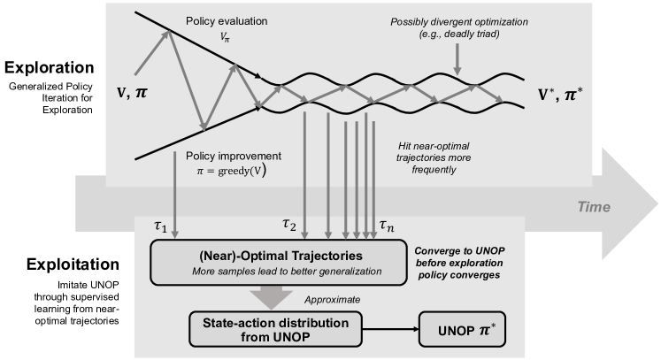
Figure 1: The off-policy learning as supervised learning framework for general policy gradient methods.

Based on the discussions in Section 5, we exploit the advantage of reducing RL into supervised learning via a proposed two-stages off-policy learning framework. As we illustrated in Figure 1, the proposed framework contains the following two stages:

Generalized Policy Iteration for Exploration. The goal of the exploration stage is to collect different near-optimal trajectories as frequently as possible. Under the off-policy framework, the exploration agent and the learning agent can be separated. Therefore, any existing RL algorithm can be used during the exploration. The principle of this framework is using the most advanced RL agents as an exploration strategy in order to collect more near-optimal trajectories and leave the policy learning to the supervision stage.

Supervision. In this stage, we imitate the uniformly near-optimal policy, UNOP (Def 11). Although we have no access to the UNOP, we can approximate the state-action distribution from UNOP by collecting the near-optimal trajectories only. The near-optimal samples are constructed online and we are not given any expert demonstration or expert policy beforehand. This step provides a sample-efficient approach to conduct exploitation, which enjoys the superiority of stability (Figure 3), variance reduction (Corollary 17), and optimality preserving (Theorem 12).

The two-stage algorithmic framework can be directly incorporated in RPG and LPG to improve sample efficiency. The implementation of RPG is given in Algorithm 1, and LPG follows the same procedure except for the difference in the loss function. The main requirement of Alg. 1 is on the exploration efficiency and the MDP structure. During the exploration stage, a sufficient amount of the different near-optimal trajectories need to be collected for constructing a representative supervised learning training dataset. Theoretically, this requirement always holds [see Appendix Section G, Lemma 33], while the number of episodes explored could be prohibitively large, which makes this algorithm sample-inefficient. This could be a practical concern of the proposed algorithm. However, according to our extensive empirical observations, we notice that long before the value function based state-of-the-art converges to near-optimal performance, enough amount of near-optimal trajectories are already explored.

Therefore, we point out that instead of estimating optimal action value functions and then choosing action greedily, using value function to facilitate the exploration and imitating UNOP is a more sample-efficient approach. As illustrated in Figure 1, value based methods with off-policy learning, bootstrapping, and function approximation could lead to a divergent optimization (Sutton and Barto, 2018, Chap. 11). In contrast to resolving the instability, we circumvent this issue via constructing a stationary target using the samples from (near)-optimal trajectories, and perform imitation learning. This two-stage approach can avoid the extensive exploration of the suboptimal state-action space and reduce the substantial number of samples needed for estimating optimal action values. In the MDP where we have a high probability of hitting the near-optimal trajectories (such as Pong), the supervision stage can further facilitate the exploration. It should be emphasized that our work focuses on improving the sample-efficiency through more effective exploitation, rather than developing novel exploration method.

0:  The near-optimal trajectory reward threshold $c$, the number of maximal training episodes $N_{max}$. Maximum number of time steps in each episode $T$, and batch size $b$.

1:  while  episode $<N_{\max}$ do

2:    repeat

3:       Retrieve state $s_{t}$ and sample action $a_{t}$ by the specified exploration agent (can be random, $\epsilon$-greedy, or any RL algorithms).

4:       Collect the experience $e_{t}=(s_{t},a_{t},r_{t},s_{t+1})$ and store to the replay buffer.

5:       $t=t+1$

6:       if t % update step == 0 then

7:          Sample a batch of experience $\{e_{j}\}_{j=1}^{b}$ from the near-optimal replay buffer.

8:          Update $\pi_{\theta}$ based on the hinge loss Eq (11) for RPG.

9:          Update the exploration agent using samples from the regular replay buffer (In simple MDPs such as Pong where near-optimal trajectories are encountered frequently, near-optimal replay buffer can be used to update the exploration agent).

10:       end if

11:    until terminal $s_{t}$ or $t-t_{\text{start}}>=T$

12:    if return $\sum_{t=1}^{T}r_{t}\geq c$ then

13:       Take the near-optimal trajectory $e_{t},t=1,...,T$ in the latest episode from the regular replay buffer, and insert the trajectory into the near-optimal replay buffer.

14:    end if

15:    if $t$ % evaluation step == 0 then

16:       Evaluate the RPG agent by greedily choosing the action. If the best performance is reached, then stop training.

17:    end if

18:  end while

Algorithm 1 Off-Policy Learning for Ranking Policy Gradient (RPG)

7 Sample Complexity and Generalization Performance

In this section, we present a theoretical analysis on the sample complexity of RPG with off-policy learning framework in Section 6. The analysis leverages the results from the Probably Approximately Correct (PAC) framework, and provides an alternative approach to quantify sample complexity of RL from the perspective of the connection between RL and SL (see Theorem 12), which is significantly different from the existing approaches that use value function estimations (Kakade et al., 2003; Strehl et al., 2006; Kearns et al., 2000; Strehl et al., 2009; Krishnamurthy et al., 2016; Jiang et al., 2017; Jiang and Agarwal, 2018; Zanette and Brunskill, 2019). We show that the sample complexity of RPG (Theorem 19) depends on the properties of MDP such as horizon, action space, dynamics, and the generalization performance of supervised learning. It is worth mentioning that the sample complexity of RPG has no linear dependence on the state-space, which makes it suitable for large-scale MDPs. Moreover, we also provide a formal quantitative definition (Def 21) on the exploration efficiency of RL.

Corresponding to the two-stage framework in Section 6, the sample complexity of RPG also splits into two problems:

• Learning efficiency: How many state-action pairs from the uniformly optimal policy do we need to collect, in order to achieve good generalization performance in RL?

• Exploration efficiency: For a certain type of MDPs, what is the probability of collecting $n$ training samples (state-action pairs from the uniformly near-optimal policy) in the first $k$ episodes in the worst case? This question leads to a quantitative evaluation metric of different exploration methods.

The first stage is resolved by Theorem 19, which connects the lower bound of the generalization performance of RL to the supervised learning generalization performance. Then we discuss the exploration efficiency of the worst case performance for a binary tree MDP in Lemma 23. Jointly, we show how to link the two stages to give a general theorem that studies how many samples we need to collect in order to achieve certain performance in RL.

In this section, we restrict our discussion on the MDPs with a fixed action space and assume the existence of deterministic optimal policy. The policy $\pi=\hat{h}=\operatorname*{arg\,min}_{h\in{\mathcal{H}}}\hat{\epsilon}(h)$ corresponds to the empirical risk minimizer (ERM) in the learning theory literature, which is the policy we obtained through learning on the training samples. ${\mathcal{H}}$ denotes the hypothesis class from where we are selecting the policy. Given a hypothesis (policy) $h$, the empirical risk is given by $\hat{\epsilon}(h)=\sum_{i=1}^{n}\frac{1}{n}\textbf{1}\{h(s_{i})\neq a_{i}\}$. Without loss of generosity, we can normalize the reward function to set the upper bound of trajectory reward equals to one ($i.e.,R_{\max}=1$), similar to the assumption in (Jiang and Agarwal, 2018). It is worth noting that the training samples are generated i.i.d. from an unknown distribution, which is perhaps the most important assumption in the statistical learning theory. i.i.d. is satisfied in this case since the state action pairs (training samples) are collected by filtering the samples during the learning stage, and we can manually manipulate the samples to follow the distribution of UOP (Def 11) by only storing the unique near-optimal trajectories.

7.1 Supervision stage: Learning efficiency

To simplify the presentation, we restrict our discussion on the finite hypothesis class (i.e. $|{\mathcal{H}}|<\infty$) since this dependence is not germane to our discussion. However, we note that the theoretical framework in this section is not limited to the finite hypothesis class. For example, we can simply use the VC dimension (Vapnik, 2006) or the Rademacher complexity (Bartlett and Mendelson, 2002) to generalize our discussion to the infinite hypothesis class, such as neural networks. For completeness, we first revisit the sample complexity result from the PAC learning in the context of RL.

Lemma 18 (Supervised Learning Sample Complexity (Mohri et al., 2018))

Let $|{\mathcal{H}}|<\infty$, and let $\delta,\gamma$ be fixed, the inequality $\epsilon(\hat{h})\leq(\min_{h\in{\mathcal{H}}}\epsilon(h))+2\gamma=\eta$ holds with probability at least $1-\delta$, when the training set size $n$ satisfies:

$$n\geq\frac{1}{2\gamma^{2}}\log\frac{2|{\mathcal{H}}|}{\delta},$$ (13)

where the generalization error (expected risk) of a hypothesis $\hat{h}$ is defined as:

$$\epsilon(\hat{h})=\sum_{s,a}\nolimits p_{\pi_{*}}(s,a)\textbf{1}\left\{\hat{h}(s)\neq a\right\}.$$

Condition 1 (Action values)

We restrict the action values of RPG in certain range, i.e., $\lambda_{i}\in[0,c_{q}]$, where $c_{q}$ is a positive constant.

This condition can be easily satisfied, for example, we can use a sigmoid to cast the action values into $[0,1]$. We can impose this constraint since in RPG we only focus on the relative relationship of action values. Given the mild condition and established on the prior work in statistical learning theory, we introduce the following results that connect the supervised learning and reinforcement learning.

Theorem 19 (Generalization Performance)

Given a MDP where the UOP (Def 11) is deterministic, let $|{\mathcal{H}}|$ denote the size of hypothesis space, and $\delta,n$ be fixed, the following inequality holds with probability at least $1-\delta$:

$$\sum_{\tau}\nolimits p_{\theta}(\tau)r(\tau)\geq D(1+e)^{\eta(1-m)T},$$

where $D=|{\mathcal{T}}|\left(\Pi_{\tau\in{\mathcal{T}}}p_{d}(\tau)\right)^{\frac{1}{|{\mathcal{T}}|}}$, $p_{d}(\tau)=p(s_{1})\Pi_{t=1}^{T}p(s_{t+1}|s_{t},a_{t})$ denotes the environment dynamics. $\eta$ is the upper bound of supervised learning generalization performance, defined as $\eta=(\min_{h\in{\mathcal{H}}}\epsilon(h))+2\sqrt{\frac{1}{2n}\log\frac{2|{\mathcal{H}}|}{\delta}}=2\sqrt{\frac{1}{2n}\log\frac{2|{\mathcal{H}}|}{\delta}}$.

Corollary 20 (Sample Complexity)

Given a MDP where the UOP (Def 11) is deterministic, let $|{\mathcal{H}}|$ denotes the size of hypothesis space, and let $\delta$ be fixed. Then for the following inequality to hold with probability at least $1-\delta$:

$$\sum\nolimits_{\tau}p_{\theta}(\tau)r(\tau)\geq 1-\epsilon,$$

it suffices that the number of state action pairs (training sample size $n$) from the uniformly optimal policy satisfies:

$$n\geq\frac{2(m-1)^{2}T^{2}}{(\log_{1+e}\frac{D}{1-\epsilon})^{2}}\log\frac{2|{\mathcal{H}}|}{\delta}=\mathcal{O}\left(\frac{m^{2}T^{2}}{\left(\log\frac{D}{1-\epsilon}\right)^{2}}\log\frac{|{\mathcal{H}}|}{\delta}\right).$$

The proofs of Theorem 19 and Corollary 20 are provided in Appendix I. Theorem 19 establishes the connection between the generalization performance of RL and the sample complexity of supervised learning. The lower bound of generalization performance decreases exponentially with respect to the horizon $T$ and action space dimension $m$. This is aligned with our empirical observation that it is more difficult to learn the MDPs with a longer horizon and/or a larger action space. Furthermore, the generalization performance has a linear dependence on $D$, the transition probability of optimal trajectories. Therefore, $T$, $m$, and $D$ jointly determines the difficulty of learning of the given MDP. As pointed out by Corollary 20, the smaller the $D$ is, the higher the sample complexity. Note that $T$, $m$, and $D$ all characterize intrinsic properties of MDPs, which cannot be improved by our learning algorithms. One advantage of RPG is that its sample complexity has no dependence on the state space, which enables the RPG to resolve large-scale complicated MDPs, as demonstrated in our experiments. In the supervision stage, our goal is the same as in the traditional supervised learning: to achieve better generalization performance $\eta$.

7.2 Exploration stage: Exploration efficiency

The exploration efficiency is highly related to the MDP properties and the exploration strategy. To provide interpretation on how the MDP properties (state space dimension, action space dimension, horizon) affect the sample complexity through exploration efficiency, we characterize a simplified MDP as in (Sun et al., 2017) , in which we explicitly compute the exploration efficiency of a stationary policy (random exploration), as shown in Figure 2.

Definition 21 (Exploration Efficiency)

We define the exploration efficiency of a certain exploration algorithm ($A$) within a MDP (${\mathcal{M}}$) as the probability of sampling $i$ distinct optimal trajectories in the first $k$ episodes. We denote the exploration efficiency as $p_{A,{\mathcal{M}}}(n_{traj}\geq i|k)$. When ${\mathcal{M}}$, $k$, $i$ and optimality threshold $c$ are fixed, the higher the $p_{A,{\mathcal{M}}}(n_{traj}\geq i|k)$, the better the exploration efficiency. We use $n_{traj}$ to denote the number of near-optimal trajectories in this subsection. If the exploration algorithm derives a series of learning policies, then we have $p_{A,{\mathcal{M}}}(n_{traj}\geq i|k)=p_{\{\pi_{i}\}_{i=0}^{t},{\mathcal{M}}}(n_{traj}\geq i|k)$, where $t$ is the number of steps the algorithm $A$ updated the policy. If we would like to study the exploration efficiency of a stationary policy, then we have $p_{A,{\mathcal{M}}}(n_{traj}\geq i|k)=p_{\pi,{\mathcal{M}}}(n_{traj}\geq i|k)$.

Definition 22 (Expected Exploration Efficiency)

The expected exploration efficiency of a certain exploration algorithm ($A$) within a MDP (${\mathcal{M}}$) is defined as:

$$E_{A,k,{\mathcal{M}}}=\sum\nolimits_{i=0}^{k}p_{A,{\mathcal{M}}}(n_{traj}=i|k)i.$$

The definitions provide a quantitative metric to evaluate the quality of exploration. Intuitively, the quality of exploration should be determined by how frequently it will hit different good trajectories. We use Def 21 for theoretical analysis and Def 22 for practical evaluation.

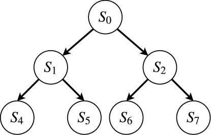
Figure 2: The binary tree structure MDP (${\mathcal{M}}_{1}$) with one initial state, similar as discussed in (Sun et al., 2017). In this subsection, we focus on the MDPs that have no duplicated states. The initial state distribution of the MDP is uniform and the environment dynamics is deterministic. For ${\mathcal{M}}_{1}$ the worst case exploration is random exploration and each trajectory will be visited at same probability under random exploration. Note that in this type of MDP, the Assumption 2 is satisfied.

Lemma 23 (The Exploration Efficiency of Random Policy)

The Exploration Efficiency of random exploration policy in a binary tree MDP (${\mathcal{M}}_{1}$) is given as:

$$p_{\pi_{r},{\mathcal{M}}}(n_{traj}\geq i|k)=1-\sum_{i^{\prime}=0}^{i-1}\nolimits C_{|{\mathcal{T}}|}^{i^{\prime}}\frac{\sum_{j=0}^{i^{\prime}}(-1)^{j}C_{i^{\prime}}^{j}(N-|{\mathcal{T}}|+i^{\prime}-j)^{k}}{N^{k}},$$

where $N$ denotes the total number of different trajectories in the MDP. In binary tree MDP ${\mathcal{M}}_{1}$, $N=|{\mathcal{S}}_{0}||{\mathcal{A}}|^{T}$, where the $|{\mathcal{S}}_{0}|$ denotes the number of distinct initial states. $|{\mathcal{T}}|$ denotes the number of optimal trajectories. $\pi_{r}$ denotes the random exploration policy, which means the probability of hitting each trajectory in ${\mathcal{M}}_{1}$ is equal.

The proof of Lemma 23 is available in Appendix J.

7.3 Joint Analysis Combining Exploration and Supervision

In this section, we jointly consider the learning efficiency and exploration efficiency to study the generalization performance. Concretely, we would like to study if we interact with the environment a certain number of episodes, what is the worst generalization performance we can expect with certain probability, if RPG is applied.

Corollary 24 (RL Generalization Performance)

Given a MDP where the UOP (Def 11) is deterministic, let $|{\mathcal{H}}|$ be the size of the hypothesis space, and let $\delta,n,k$ be fixed, the following inequality holds with probability at least $1-\delta^{\prime}$:

$$\sum_{\tau}\nolimits p_{\theta}(\tau)r(\tau)\geq D(1+e)^{\eta(1-m)T},$$

where $k$ is the number of episodes we have explored in the MDP, $n$ is the number of distinct optimal state-action pairs we needed from the UOP (i.e., size of training data.). $n^{\prime}$ denotes the number of distinct optimal state-action pairs collected by the random exploration. $\eta=2\sqrt{\frac{1}{2n}\log\frac{2|{\mathcal{H}}|p_{\pi_{r},{\mathcal{M}}}(n^{\prime}\geq n|k)}{p_{\pi_{r},{\mathcal{M}}}(n^{\prime}\geq n|k)-1+\delta^{\prime}}}$.

The proof of Corollary 24 is provided in Appendix K. Corollary 24 states that the probability of sampling optimal trajectories is the main bottleneck of exploration and generalization, instead of state space dimension. In general, the optimal exploration strategy depends on the properties of MDPs. In this work, we focus on improving learning efficiency, i.e., learning optimal ranking instead of estimating value functions. The discussion of optimal exploration is beyond the scope of this work.

8 Experimental Results

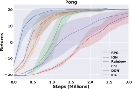
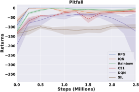
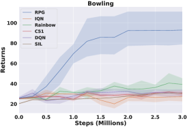
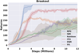
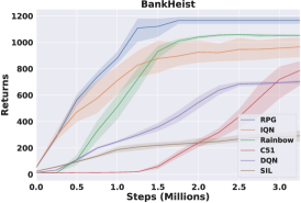
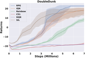
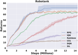
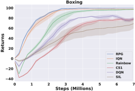
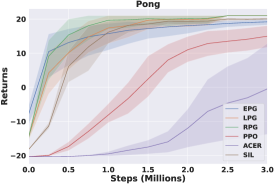
Figure 3: The training curves of the proposed RPG and state-of-the-art. All results are averaged over random seeds from 1 to 5. The $x$-axis represents the number of steps interacting with the environment (we update the model every four steps) and the $y$-axis represents the averaged training episodic return. The error bars are plotted with a confidence interval of 95%.

To evaluate the sample-efficiency of Ranking Policy Gradient (RPG), we focus on Atari 2600 games in OpenAI gym (Bellemare et al., 2013; Brockman et al., 2016), without randomly repeating the previous action. We compare our method with the state-of-the-art baselines including DQN (Mnih et al., 2015), C51 (Bellemare et al., 2017), IQN (Dabney et al., 2018), Rainbow (Hessel et al., 2017), and self-imitation learning (SIL) (Oh et al., 2018). For reproducibility, we use the implementation provided in Dopamine framework (Castro et al., 2018) for all baselines and proposed methods, except for SIL using the official implementation. . Follow the standard practice (Oh et al., 2018; Hessel et al., 2017; Dabney et al., 2018; Bellemare et al., 2017), we report the training performance of all baselines as the increase of interactions with the environment, or proportionally the number of training iterations. We run the algorithms with five random seeds and report the average rewards with $95$% confidence intervals. The implementation details of the proposed RPG and its variants are given as follows:

EPG: EPG is the stochastic listwise policy gradient (see Eq (7)) incorporated with the proposed off-policy learning. More concretely, we apply trajectory reward shaping (TRS, Def 7) to all trajectories encountered during exploration and train vanilla policy gradient using the off-policy samples. This is equivalent to minimizing the cross-entropy loss (see Appendix Eq (12)) over the near-optimal trajectories.

LPG: LPG is the deterministic listwise policy gradient with the proposed off-policy learning. The only difference between EPG and LPG is that LPG chooses action deterministically (see Appendix Eq (6)) during evaluation.

RPG: RPG explores the environment using a separate EPG agent in Pong and IQN in other games. Then RPG conducts supervised learning by minimizing the hinge loss Eq (11). It is worth noting that the exploration agent (EPG or IQN) can be replaced by any existing exploration method. In our RPG implementation, we collect all trajectories with the trajectory reward no less than the threshold $c$ without eliminating the duplicated trajectories and we empirically found it is a reasonable simplification.

Sample-efficiency. As the results shown in Figure 3, our approach, RPG, significantly outperforms the state-of-the-art baselines in terms of sample-efficiency at all tasks. Furthermore, RPG not only achieved the most sample-efficient results, but also reached the highest final performance at Robotank, DoubleDunk, Pitfall, and Pong, comparing to any model-free state-of-the-art. In reinforcement learning, the stability of algorithm should be emphasized as an important issue. As we can see from the results, the performance of baselines varies from task to task. There is no single baseline consistently outperforms others. In contrast, due to the reduction from RL to supervised learning, RPG is consistently stable and effective across different environments. In addition to the stability and efficiency, RPG enjoys simplicity at the same time. In the environment Pong, it is surprising that RPG without any complicated exploration method largely surpassed the sophisticated value-function based approaches. More details of hyperparameters are provided in the Appendix Section K.1.

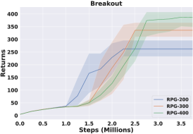
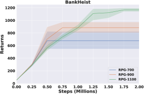
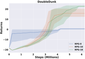
Figure 4: The trade-off between sample efficiency and optimality on DoubleDunk,BreakOut, BankHeist. As the trajectory reward threshold ($c$) increase, more samples are needed for the learning to converge, while it leads to better final performance. We denote the value of $c$ by the numbers at the end of legends.

8.1 Ablation Study

The effectiveness of pairwise ranking policy and off-policy learning as supervised learning. To get a better understanding of the underlying reasons that RPG is more sample-efficient than DQN variants, we performed ablation studies in the Pong environment by varying the combination of policy functions with the proposed off-policy learning. The results of EPG, LPG, and RPG are shown in the bottom right, Figure 3. Recall that EPG and LPG use listwise policy gradient (vanilla policy gradient using softmax as policy function) to conduct exploration, the off-policy learning minimizes the cross-entropy loss Eq (12). In contrast, RPG shares the same exploration method as EPG and LPG while uses pairwise ranking policy Eq (2) in off-policy learning that minimizes hinge loss Eq (11). We can see that RPG is more sample-efficient than EPG/LPG in learning deterministic optimal policy. We also compared the advanced on-policy method Proximal Policy Optimization (PPO) (Schulman et al., 2017) with EPG, LPG, and RPG. The proposed off-policy learning largely surpassed the best on-policy method. Therefore, we conclude that off-policy as supervised learning contributes to the sample-efficiency substantially, while the pairwise ranking policy can further accelerate the learning. In addition, we compare RPG to representative off-policy policy gradient approach: ACER (Wang et al., 2016). As the results shown, the proposed off-policy learning framework is more sample-efficient than the state-of-the-art off-policy policy gradient approaches.

On the Trade-off between Sample-Efficiency and Optimality. Results in Figure 4 show that there is a trade-off between sample efficiency and optimality, which is controlled by the trajectory reward threshold $c$. Recall that $c$ determines how close is the learned UNOP to optimal policies. A higher value of $c$ leads to a less frequency of near-optimal trajectories being collected and and thus a lower sample efficiency, and however the algorithm is expected to converge to a strategy of better performance. We note that $c$ is the only parameter we tuned across all experiments.

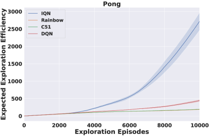
Figure 5: The expected exploration efficiency of state-of-the-art, the results are averaged over random seeds from 1 to 10.

Exploration Efficiency. We empirically evaluate the Expected Exploration Efficiency (Def 21) of the state-of-the-art on Pong. It is worth noting that the RL generalization performance is determined by both of learning efficiency and exploration efficiency. Therefore, higher exploration efficiency does not necessarily lead to more sample efficient algorithm due to the learning inefficiency, as demonstrated by RainBow and DQN (see Figure 5). Also, the Implicit Quantile achieves the best performance among baselines, since its exploration efficiency largely surpasses other baselines.

9 Conclusions

In this work, we introduced ranking policy gradient methods that, for the first time, approach the RL problem from a ranking perspective. Furthermore, towards the sample-efficient RL, we propose an off-policy learning framework, which trains RL agents in a supervised learning manner and thus largely facilitates the learning efficiency. The off-policy learning framework uses generalized policy iteration for exploration and exploits the stableness of supervised learning for deriving policy, which accomplishes the unbiasedness, variance reduction, off-policy learning, and sample efficiency at the same time. Besides, we provide an alternative approach to analyze the sample complexity of RL, and show that the sample complexity of RPG has no dependency on the state space dimension. Last but not least, empirical results show that RPG achieves superior performance as compared to the state-of-the-art.

Appendix A Discussion of Existing Efforts on Connecting Reinforcement Learning to Supervised Learning.

There are two main distinctions between supervised learning and reinforcement learning. In supervised learning, the data distribution ${\mathcal{D}}$ is static and training samples are assumed to be sampled i.i.d. from ${\mathcal{D}}$. On the contrary, the data distribution is dynamic in reinforcement learning and the sampling procedure is not independent. First, since the data distribution in RL is determined by both environment dynamics and the learning policy, and the policy keeps being updated during the learning process. This updated policy results in dynamic data distribution in reinforcement learning. Second, policy learning depends on previously collected samples, which in turn determines the sampling probability of incoming data. Therefore, the training samples we collected are not independently distributed. These intrinsic difficulties of reinforcement learning directly cause the sample-inefficient and unstable performance of current algorithms.

On the other hand, most state-of-the-art reinforcement learning algorithms can be shown to have a supervised learning equivalent. To see this, recall that most reinforcement learning algorithms eventually acquire the policy either explicitly or implicitly, which is a mapping from a state to an action or a probability distribution over the action space. The use of such a mapping implies that ultimately there exists a supervised learning equivalent to the original reinforcement learning problem, if optimal policies exist. The paradox is that it is almost impossible to construct this supervised learning equivalent on the fly, without knowing any optimal policy.

Although the question of how to construct and apply proper supervision is still an open problem in the community, there are many existing efforts providing insightful approaches to reduce reinforcement learning into its supervised learning counterpart over the past several decades. Roughly, we can classify the existing efforts into the following categories:

• Expectation-Maximization (EM): Dayan and Hinton (1997); Peters and Schaal (2007); Kober and Peters (2009); Abdolmaleki et al. (2018), etc.

• Entropy-Regularized RL (ERL): O’Donoghue et al. (2016); Oh et al. (2018); Haarnoja et al. (2018), etc.

• Interactive Imitation Learning (IIL): Daumé et al. (2009); Syed and Schapire (2010); Ross and Bagnell (2010); Ross et al. (2011); Sun et al. (2017), etc.

The early approaches in the EM track applied Jensen’s inequality and approximation techniques to transform the reinforcement learning objective. Algorithms are then derived from the transformed objective, which resemble the Expectation-Maximization procedure and provide policy improvement guarantee (Dayan and Hinton, 1997). These approaches typically focus on a simplified RL setting, such as assuming that the reward function is not associated with the state (Dayan and Hinton, 1997), approximating the goal to maximize the expected immediate reward and the state distribution is assumed to be fixed (Peters and Schaal, 2008). Later on in Kober and Peters (2009), the authors extended the EM framework from targeting immediate reward into episodic return. Recently, Abdolmaleki et al. (2018) used the EM-framework on a relative entropy objective, which adds a parameter prior as regularization. It has been found that the estimation step using Retrace (Munos et al., 2016) can be unstable even with a linear function approximation (Touati et al., 2017). In general, the estimation step in EM-based algorithms involves on-policy evaluation, which is one challenge shared among policy gradient methods. On the other hand, off-policy learning usually leads to a much better sample efficiency, and is one main motivation that we want to reformulate RL into a supervised learning task.

To achieve off-policy learning, PGQ (O’Donoghue et al., 2016) connected the entropy-regularized policy gradient with Q-learning under the constraint of small regularization. In the similar framework, Soft Actor-Critic  (Haarnoja et al., 2018) was proposed to enable sample-efficient and faster convergence under the framework of entropy-regularized RL. It is able to converge to the optimal policy that optimizes the long-term reward along with policy entropy. It is an efficient way to model the suboptimal behavior and empirically it is able to learn a reasonable policy. Although recently the discrepancy between the entropy-regularized objective and original long-term reward has been discussed in (O’Donoghue, 2018; Eysenbach and Levine, 2019), they focus on learning stochastic policy while the proposed framework is feasible for both learning deterministic optimal policy (Corollary 15) and stochastic optimal policy (Corollary 16). In (Oh et al., 2018), this work shares similarity to our work in terms of the method we collecting the samples. They collect good samples based on the past experience and then conduct the imitation learning w.r.t those good samples. However, we differentiate at how do we look at the problem theoretically. This self-imitation learning procedure was eventually connected to lower-bound-soft-Q-learning, which belongs to entropy-regularized reinforcement learning. We comment that there is a trade-off between sample-efficiency and modeling suboptimal behaviors. The more strict requirement we have on the samples collected we have less chance to hit the samples while we are more close to imitating the optimal behavior.

Methods	Objective	Cont. Action	Optimality	Off-Policy	No Oracle
EM	✓	✓	✓	✗	✓
ERL	✗	✓	✓†	✓	✓
IIL	✓	✓	✓	✓	✗
RPG	✓	✗	✓	✓	✓

Table 2: A comparison of studies reducing RL to SL. The Objective column denotes whether the goal is to maximize long-term reward. The Cont. Action column denotes whether the method is applicable to both continuous and discrete action spaces. The Optimality denotes whether the algorithms can model the optimal policy. ✓^† denotes the optimality achieved by ERL is w.r.t. the entropy regularize objective instead of the original objective on return. The Off-Policy column denotes if the algorithms enable off-policy learning. The No Oracle column denotes if the algorithms need to access to a certain type of oracle (expert policy or expert demonstrations).

From the track of interactive imitation learning, early efforts such as (Ross and Bagnell, 2010; Ross et al., 2011) pointed out that the main discrepancy between imitation learning and reinforcement learning is the violation of i.i.d. assumption. SMILe (Ross and Bagnell, 2010) and DAgger (Ross et al., 2011) are proposed to overcome the distribution mismatch. Theorem 2.1 in Ross and Bagnell (2010) quantified the performance degradation from the expert considering that the learned policy fails to imitate the expert with a certain probability. The theorem seems to resemble the long-term performance theorem (Thm. 12) in this paper. However, it studied the scenario that the learning policy is trained through a state distribution induced by the expert, instead of state-action distribution as considered in Theorem 12. As such, Theorem 2.1 in Ross and Bagnell (2010) may be more applicable to the situation where an interactive procedure is needed, such as querying the expert during the training process. On the contrary, the proposed work focuses on directly applying supervised learning without having access to the expert to label the data. The optimal state-action pairs are collected during exploration and conducting supervised learning on the replay buffer will provide a performance guarantee in terms of long-term expected reward. Concurrently, a resemble of Theorem 2.1 in (Ross and Bagnell, 2010) is Theorem 1 in (Syed and Schapire, 2010), where the authors reduced the apprenticeship learning to classification, under the assumption that the apprentice policy is deterministic and the misclassification rate is bounded at all time steps. In this work, we show that it is possible to circumvent such a strong assumption and reduce RL to its SL. Furthermore, our theoretical framework also leads to an alternative analysis of sample-complexity. Later on AggreVaTe (Ross and Bagnell, 2014) was proposed to incorporate the information of action costs to facilitate imitation learning, and its differentiable version AggreVaTeD (Sun et al., 2017) was developed in succession and achieved impressive empirical results. Recently, hinge loss was introduced to regular $Q$-learning as a pre-training step for learning from demonstration (Hester et al., 2018), or as a surrogate loss for imitating optimal trajectories (Osa et al., 2018). In this work, we show that hinge loss constructs a new type of policy gradient method and can be used to learn optimal policy directly.

In conclusion, our method approaches the problem of reducing RL to SL from a unique perspective that is different from all prior work. With our reformulation from RL to SL, the samples collected in the replay buffer satisfy the i.i.d. assumption, since the state-action pairs are now sampled from the data distribution of UNOP. A multi-aspect comparison between the proposed method and relevant prior studies is summarized in Table 2.

Appendix B Ranking Policy Gradient Theorem

The Ranking Policy Gradient Theorem (Theorem 4) formulates the optimization of long-term reward using a ranking objective. The proof below illustrates the formulation process.

Proof  The following proof is based on direct policy differentiation (Peters and Schaal, 2008; Williams, 1992). For a concise presentation, the subscript $t$ for action value $\lambda_{i},\lambda_{j}$, and $p_{ij}$ is omitted.

$${\nabla}_{\theta}J({\theta})= {\nabla}_{\theta}\sum_{\tau}\nolimits p_{\theta}(\tau)r(\tau)$$ (14)

$$= \sum_{\tau}\nolimits p_{\theta}(\tau){\nabla}_{\theta}\log p_{\theta}(\tau)r(\tau)$$

$$= \sum_{\tau}\nolimits p_{\theta}(\tau){\nabla}_{\theta}\log\left(p(s_{0})\Pi_{t=1}^{T}\pi_{\theta}(a_{t}|s_{t})p(s_{t+1}|s_{t},a_{t})\right)r(\tau)$$

$$= \sum_{\tau}\nolimits p_{\theta}(\tau)\sum_{t=1}^{T}\nolimits{\nabla}_{\theta}\log\pi_{\theta}(a_{t}|s_{t})r(\tau)$$

$$= {\mathbf{E}}_{\tau\sim\pi_{\theta}}\left[\sum_{t=1}^{T}\nolimits{\nabla}_{\theta}\log\pi_{\theta}(a_{t}|s_{t})r(\tau)\right]$$

$$= {\mathbf{E}}_{\tau\sim\pi_{\theta}}\left[\sum_{t=1}^{T}\nolimits{\nabla}_{\theta}\log\left(\prod\nolimits_{j=1,j\neq i}^{m}p_{ij}\right)r(\tau)\right]$$

$$= {\mathbf{E}}_{\tau\sim\pi_{\theta}}\left[\sum_{t=1}^{T}\nolimits{\nabla}_{\theta}\sum_{j=1,j\neq i}^{m}\nolimits\log\left(\frac{e^{\lambda_{ij}}}{1+e^{\lambda_{ij}}}\right)r(\tau)\right]$$

$$= {\mathbf{E}}_{\tau\sim\pi_{\theta}}\left[\sum_{t=1}^{T}\nolimits{\nabla}_{\theta}\sum_{j=1,j\neq i}^{m}\nolimits\log\left(\frac{1}{1+e^{\lambda_{ji}}}\right)r(\tau)\right]$$ (15)

$$\approx {\mathbf{E}}_{\tau\sim\pi_{\theta}}\left[\sum_{t=1}^{T}\nolimits{\nabla}_{\theta}\left(\sum_{j=1,j\neq i}^{m}\nolimits(\lambda_{i}-\lambda_{j})/2\right)r(\tau)\right],$$ (16)

where the trajectory is a series of state-action pairs from $t=1,...,T$, $i.e.\tau=s_{1},a_{1},s_{2},a_{2},...,s_{T}$. From Eq (15) to Eq (16), we use the first-order Taylor expansion of $\log(1+e^{x})|_{x=0}=\log 2+\frac{1}{2}x+O(x^{2})$ to further simplify the ranking policy gradient.  

B.1 Probability Distribution in Ranking Policy Gradient

In this section, we discuss the output property of the pairwise ranking policy. We show in Corollary 25 that the pairwise ranking policy gives a valid probability distribution when the dimension of the action space $m=2$. For cases when $m>2$ and the range of $Q$-value satisfies Condition 2, we show in Corollary 26 how to construct a valid probability distribution.

Corollary 25

The pairwise ranking policy as shown in Eq (2) constructs a probability distribution over the set of actions when the action space $m$ is equal to $2$, given any action values $\lambda_{i},i=1,2$. For the cases with $m>2$, this conclusion does not hold in general.

It is easy to verify that $\pi(a_{i}|s)>0$, $\sum_{i=1}^{2}\pi(a_{i}|s)=1$ holds and the same conclusion cannot be applied to $m>2$ by constructing counterexamples. However, we can introduce a dummy action $a^{\prime}$ to form a probability distribution for RPG. During policy learning, the algorithm increases the probability of best actions and the probability of dummy action decreases. Ideally, if RPG converges to an optimal deterministic policy, the probability of taking best action is equal to 1 and $\pi(a^{\prime}|s)=0$. Similarly, we can introduce a dummy trajectory $\tau^{\prime}$ with the trajectory reward $r(\tau^{\prime})=0$ and $p_{\theta}(\tau^{\prime})=1-\sum_{\tau}p_{\theta}(\tau)$. The trajectory probability forms a probability distribution since $\sum_{\tau}p_{\theta}(\tau)+p_{\theta}(\tau^{\prime})=1$ and $p_{\theta}(\tau)\geq 0\ \forall\tau$ and $p_{\theta}(\tau^{\prime})\geq 0$. The proof of a valid trajectory probability is similar to the following proof on $\pi(a|s)$ to be a valid probability distribution with a dummy action. Its practical influence is negligible since our goal is to increase the probability of (near)-optimal trajectories. To present in a clear way, we avoid mentioning dummy trajectory $\tau^{\prime}$ in Proof B while it can be seamlessly included.

Condition 2 (The range of action-value)

We restrict the range of action-values in RPG so that it satisfies $\lambda_{m}\geq\ln(m^{\frac{1}{m-1}}-1)$, where $\lambda_{m}=\min_{i,j}\lambda_{ji}$ and $m$ is the dimension of the action space.

This condition can be easily satisfied since in RPG we only focus on the relative relationship of $\lambda$ and we can constrain the range of action-values so that $\lambda_{m}$ satisfies the condition 2. Furthermore, since we can see that $m^{\frac{1}{m-1}}>1$ is decreasing w.r.t to action dimension $m$. The larger the action dimension, the less constraint we have on the action values.

Corollary 26

Given Condition 2, we introduce a dummy action $a^{\prime}$ and set $\pi(a=a^{\prime}|s)=1-\sum_{i}\pi(a=a_{i}|s)$, which constructs a valid probability distribution $\left(\pi(a|s)\right)$ over the action space ${\mathcal{A}}\cup a^{\prime}$.

Proof  Since we have $\pi(a=a_{i}|s)>0\ \forall i=1,\dots,m$ and $\sum_{i}\pi(a=a_{i}|s)+\pi(a=a^{\prime}|s)=1$. To prove that this is a valid probability distribution, we only need to show that $\pi(a=a^{\prime}|s)\geq 0,\ \forall m\geq 2$, i.e. $\sum_{i}\pi(a=a_{i}|s)\leq 1,\ \forall m\geq 2$. Let $\lambda_{m}=\min_{i,j}\lambda_{ji}$,

$$\sum_{i}\nolimits\pi(a=a_{i}|s)$$

$$= \sum_{i}\nolimits\prod\nolimits_{j=1,j\neq i}^{m}\ p_{ij}$$

$$= \sum_{i}\nolimits\prod\nolimits_{j=1,j\neq i}^{m}\frac{1}{1+e^{\lambda_{ji}}}$$

$$\leq \sum_{i}\nolimits\prod\nolimits_{j=1,j\neq i}^{m}\frac{1}{1+e^{\lambda_{m}}}$$

$$= m\left(\frac{1}{1+e^{\lambda_{m}}}\right)^{m-1}\leq 1\qquad\text{ (Condition~{}\ref{cond:qvalue})}.$$

This thus concludes the proof.  

Appendix C Condition of Preserving Optimality

The following condition describes what types of MDPs are directly applicable to the trajectory reward shaping (TRS, Def 7):

Condition 3 (Initial States)

The (near)-optimal trajectories will cover all initial states of MDP. i.e. $\{s(\tau,1)|\ \forall\tau\in{\mathcal{T}}\}=\{s(\tau,1)|\ \forall\tau\}$, where ${\mathcal{T}}=\{\tau|w(\tau)=1\}=\{\tau|r(\tau)\geq c\}$.

The MDPs satisfying this condition cover a wide range of tasks such as Dialogue System (Li et al., 2017), Go (Silver et al., 2017), video games (Bellemare et al., 2013) and all MDPs with only one initial state. If we want to preserve the optimality by TRS, the optimal trajectories of a MDP need to cover all initial states or equivalently, all initial states must lead to at least one optimal trajectory. Similarly, the near-optimality is preserved for all MDPs that its near-optimal trajectories cover all initial states.

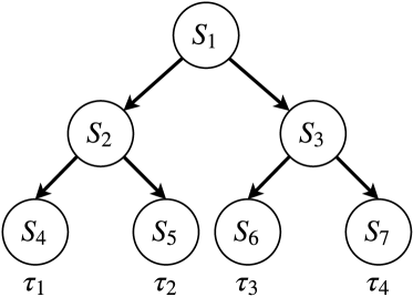
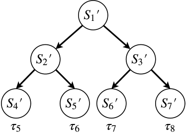
Figure 6: The binary tree structure MDP with two initial states (${\mathcal{S}}_{1}=\{s_{1},s_{1}^{\prime}\}$), similar as discussed in (Sun et al., 2017). Each path from a root to a leaf node denotes one possible trajectory in the MDP.

Theoretically, it is possible to transfer more general MDPs to satisfy Condition 3 and preserve the optimality with potential-based reward shaping (Ng et al., 1999). More concretely, consider the deterministic binary tree MDP (${\mathcal{M}}_{1}$) with the set of initial states ${\mathcal{S}}_{1}=\{s_{1},s_{1}^{\prime}\}$ as defined in Figure 6. There are eight possible trajectories in ${\mathcal{M}}_{1}$. Let $r(\tau_{1})=10=R_{\max},r(\tau_{8})=3,\ r(\tau_{i})=2,\ \forall i=2,\dots,7$. Therefore, this MDP does not satisfy Condition 3. We can compensate the trajectory reward of the best trajectory starting from $s_{1}^{\prime}$ to the $R_{\max}$ by shaping the reward with the potential-based function $\phi(s_{7}^{\prime})=7$ and $\phi(s)=0,\forall s\neq s_{7}^{\prime}$. This reward shaping requires more prior knowledge, which may not be feasible in practice. A more realistic method is to design a dynamic trajectory reward shaping approach. In the beginning, we set $c(s)=\min_{s\in{\mathcal{S}}_{1}}r(\tau|s(\tau,1)=s),\forall s\in{\mathcal{S}}_{1}$. Take ${\mathcal{M}}_{1}$ as an example, $c(s)=3,\ \forall s\in{\mathcal{S}}_{1}$. During the exploration stage, we track the current best trajectory of each initial state and update $c(s)$ with its trajectory reward.

Nevertheless, if the Condition 3 is not satisfied, we need more sophisticated prior knowledge other than a predefined trajectory reward threshold $c$ to construct the replay buffer (training dataset of UNOP). The practical implementation of trajectory reward shaping and rigorously theoretical study for general MDPs are beyond the scope of this work.

Appendix D Proof of Long-term Performance Theorem 12

Lemma 27

Given a specific trajectory $\tau$, the log-likelihood of state-action pairs over horizon $T$ is equal to the weighted sum over the entire state-action space, i.e.:

$$\frac{1}{T}\sum_{t=1}^{T}\nolimits\log\pi_{\theta}(a_{t}|s_{t})=\sum_{s,a}\nolimits p(s,a|\tau)\log\pi_{\theta}(a|s),$$

where the sum in the right hand side is the summation over all possible state-action pairs. It is worth noting that $p(s,a|\tau)$ is not related to any policy parameters. It is the probability of a specific state-action pair $(s,a)$ in a specific trajectory $\tau$.

Proof  Given a trajectory $\tau=\{(s(\tau,1),a(\tau,1)),\dots,(s(\tau,T),a(\tau,T))\}=\{(s_{1},a_{1}),\dots,(s_{T},a_{T})\}$, denote the unique state-action pairs in this trajectory as $U(\tau)=\{(s_{i},a_{i})\}_{i=1}^{n}$, where $n$ is the number of unique state-action pairs in $\tau$ and $n\leq T$. The number of occurrences of a state-action pair $(s_{i},a_{i})$ in the trajectory $\tau$ is denoted as $|(s_{i},a_{i})|$. Then we have the following:

$$\frac{1}{T}\sum_{t=1}^{T}\nolimits\log\pi_{\theta}(a_{t}|s_{t})$$

$$= \sum_{i=1}^{n}\nolimits\frac{|(s_{i},a_{i})|}{T}\log\pi_{\theta}(a_{i}|s_{i})$$

$$= \sum_{i=1}^{n}\nolimits p(s_{i},a_{i}|\tau)\log\pi_{\theta}(a_{i}|s_{i})$$

$$= \sum_{(s,a)\in U(\tau)}\nolimits p(s,a|\tau)\log\pi_{\theta}(a|s)$$ (17)

$$= \sum_{(s,a)\in U(\tau)}\nolimits p(s,a|\tau)\log\pi_{\theta}(a|s)+\sum_{(s,a)\notin U(\tau)}\nolimits p(s,a|\tau)\log\pi_{\theta}(a|s)$$ (18)

$$= \sum_{(s,a)}\nolimits p(s,a|\tau)\log\pi_{\theta}(a|s)$$

From Eq (17) to Eq (18) we used the fact:

$$\sum\nolimits_{(s,a)\in U(\tau)}p(s,a|\tau)=\sum\nolimits_{i=1}^{n}p(s_{i},a_{i}|\tau)=\sum\nolimits_{i=1}^{n}\frac{|(s_{i},a_{i})|}{T}=1,$$

and therefore we have $p(s,a|\tau)=0,\ \forall(s,a)\notin U(\tau)$. This thus completes the proof.  

Now we are ready to prove the Theorem 12:

Proof  The following proof holds for an arbitrary subset of trajectories ${\mathcal{T}}$ determined by the threshold $c$ in Def 11. The $\pi_{*}$ is associated with $c$ and this subset of trajectories. We present the following lower bound of the expected long-term performance:

$$\operatorname*{arg\,max}_{\theta}\sum_{\tau}\nolimits p_{\theta}(\tau)w(\tau)$$

$$\because w(\tau)=0,\text{if}\ \tau\notin{\mathcal{T}}$$

$$= \operatorname*{arg\,max}_{\theta}\frac{1}{|{\mathcal{T}}|}\sum_{\tau\in{\mathcal{T}}}\nolimits p_{\theta}(\tau)w(\tau)$$

$$\text{use Lemma~{}\ref{lemma:pp} }\because p_{\theta}(\tau)>0\text{ and }w(\tau)>0,\therefore\sum_{\tau\in{\mathcal{T}}}\nolimits p_{\theta}(\tau)w(\tau)>0$$

$$= \operatorname*{arg\,max}_{\theta}\log\left(\frac{1}{|{\mathcal{T}}|}\sum_{\tau\in{\mathcal{T}}}\nolimits p_{\theta}(\tau)w(\tau)\right)$$

$$\because\log\left(\sum_{i=1}^{n}\nolimits x_{i}/n\right)\geq\sum_{i=1}^{n}\nolimits\log(x_{i})/n,\forall i,x_{i}>0,\text{we have: }$$

$$\log\left(\frac{1}{|{\mathcal{T}}|}\sum_{\tau\in{\mathcal{T}}}\nolimits p_{\theta}(\tau)w(\tau)\right)\geq\sum_{\tau\in{\mathcal{T}}}\nolimits\frac{1}{|{\mathcal{T}}|}\log p_{\theta}(\tau)w(\tau),$$

where the lower bound holds when $p_{\theta}(\tau)w(\tau)=\frac{1}{|{\mathcal{T}}|},\forall\tau\in{\mathcal{T}}$. To this end, we maximize the lower bound of the expected long-term performance:

$$\operatorname*{arg\,max}_{\theta}\sum_{\tau\in{\mathcal{T}}}\nolimits\frac{1}{|{\mathcal{T}}|}\log p_{\theta}(\tau)w(\tau)$$

$$= \operatorname*{arg\,max}_{\theta}\sum_{\tau\in{\mathcal{T}}}\nolimits\log(p(s_{1})\prod\nolimits_{t=1}^{T}(\pi_{\theta}(a_{t}|s_{t})p(s_{t+1}|s_{t},a_{t}))w(\tau))$$

$$= \operatorname*{arg\,max}_{\theta}\sum_{\tau\in{\mathcal{T}}}\nolimits\log\left(p(s_{1})\prod\nolimits_{t=1}^{T}\pi_{\theta}(a_{t}|s_{t})\prod\nolimits_{t=1}^{T}p(s_{t+1}|s_{t},a_{t})w(\tau)\right)$$

$$= \operatorname*{arg\,max}_{\theta}\sum_{\tau\in{\mathcal{T}}}\nolimits\left(\log p(s_{1})+\sum\nolimits_{t=1}^{T}\log p(s_{t+1}|s_{t},a_{t})+\sum_{t=1}^{T}\nolimits\log\pi_{\theta}(a_{t}|s_{t})+\log w(\tau)\right)$$ (19)

$$\text{The above shows that }w(\tau)\text{ can be set as an arbitrary positive constant }$$

$$= \operatorname*{arg\,max}_{\theta}\frac{1}{|{\mathcal{T}}|}\sum_{\tau\in{\mathcal{T}}}\nolimits\sum_{t=1}^{T}\nolimits\log\prod\nolimits_{\theta}(a_{t}|s_{t})$$

$$= \operatorname*{arg\,max}_{\theta}\frac{1}{|{\mathcal{T}}|T}\sum_{\tau\in{\mathcal{T}}}\nolimits\sum_{t=1}^{T}\nolimits\log\prod\nolimits_{\theta}(a_{t}|s_{t})$$ (20)

$$= \operatorname*{arg\,max}_{\theta}\frac{1}{|{\mathcal{T}}|}\sum_{\tau\in{\mathcal{T}}}\nolimits\frac{1}{T}\sum_{t=1}^{T}\nolimits\log\pi_{\theta}(a_{t}|s_{t})\quad\text{ (the existence of UNOP in Assumption~{}\ref{ass:uot}) }$$

$$= \operatorname*{arg\,max}_{\theta}\sum_{\tau\in{\mathcal{T}}}\nolimits p_{\pi_{*}}(\tau)\frac{1}{T}\left(\sum_{t=1}^{T}\nolimits\log\pi_{\theta}(a_{t}|s_{t})\right)$$

$$\text{where }\pi_{*}\text{ is a UNOP (Def~{}\ref{def:uop})}\Rightarrow p_{\pi_{*}}(\tau)=0\quad\forall\tau\notin{\mathcal{T}}$$ (21)

$$\text{{Eq~{}(\ref{eq:ltpt:48})} can be established based on }\sum_{\tau\in{\mathcal{T}}}\nolimits p_{\pi_{*}}(\tau)=\sum_{\tau\in{\mathcal{T}}}\nolimits 1/|{\mathcal{T}}|=1$$

$$= \operatorname*{arg\,max}_{\theta}\sum_{\tau}\nolimits p_{\pi_{*}}(\tau)\frac{1}{T}\left(\sum\nolimits_{t=1}^{T}\log\pi_{\theta}(a_{t}|s_{t})\right)\qquad\text{(Lemma~{}\ref{lemma:tlp})}$$

$$= \operatorname*{arg\,max}_{\theta}\sum_{\tau}\nolimits p_{\pi_{*}}(\tau)\sum_{s,a}\nolimits p(s,a|\tau)\log\pi_{\theta}(a|s)$$

The 2nd sum is over all possible state-action pairs. $$(s,a)$$ represents a specific state-action pair.

$$= \operatorname*{arg\,max}_{\theta}\sum_{\tau}\nolimits\sum_{s,a}\nolimits p_{\pi_{*}}(\tau)p(s,a|\tau)\log\pi_{\theta}(a|s)$$

$$= \operatorname*{arg\,max}_{\theta}\sum_{s,a}\nolimits\sum_{\tau}\nolimits p_{\pi_{*}}(\tau)p(s,a|\tau)\log\pi_{\theta}(a|s)$$

$$= \operatorname*{arg\,max}_{\theta}\sum_{s,a}\nolimits p_{\pi_{*}}(s,a)\log\pi_{\theta}(a|s).$$ (22)

In this proof we use $s_{t}=s(\tau,t)$ and $a_{t}=a(\tau,t)$ as abbreviations, which denote the $t$-th state and action in the trajectory $\tau$, respectively. $|{\mathcal{T}}|$ denotes the number of trajectories in ${\mathcal{T}}$. We also use the definition of $w(\tau)$ to only focus on near-optimal trajectories. We set $w(\tau)=1$ for simplicity but it will not affect the conclusion if set to other constants.

Optimality: Furthermore, the optimal solution for the objective function Eq (22) is a uniformly (near)-optimal policy $\pi_{*}$.

$$\operatorname*{arg\,max}_{\theta}\sum_{s,a}\nolimits p_{\pi_{*}}(s,a)\log\pi_{\theta}(a|s)$$

$$= \operatorname*{arg\,max}_{\theta}\sum_{s}\nolimits p_{\pi_{*}}(s)\sum_{a}\nolimits\pi_{*}(a|s)\log\pi_{\theta}(a|s)$$

$$= \operatorname*{arg\,max}_{\theta}\sum_{s}\nolimits p_{\pi_{*}}(s)\sum_{a}\nolimits\pi_{*}(a|s)\log\pi_{\theta}(a|s)-\sum_{s}\nolimits p_{\pi_{*}}(s)\sum_{a}\nolimits\log\pi_{*}(a|s)$$

$$= \operatorname*{arg\,max}_{\theta}\sum_{s}\nolimits p_{\pi_{*}}(s)\sum_{a}\nolimits\nolimits\pi_{*}(a|s)\log\frac{\pi_{\theta}(a|s)}{\pi_{*}(a|s)}$$

$$= \operatorname*{arg\,max}_{\theta}\sum_{s}\nolimits p_{\pi_{*}}(s)\sum_{a}\nolimits-KL(\pi_{*}(a|s)||\pi_{\theta}(a|s))=\pi_{*}$$

Therefore, the optimal solution of  Eq (22) is also the (near)-optimal solution for the original RL problem since $\sum_{\tau}p_{\pi_{*}}(\tau)r(\tau)=\sum_{\tau\in{\mathcal{T}}}\frac{1}{|{\mathcal{T}}|}r(\tau)\geq c=R_{\max}-\epsilon$. The optimal solution is obtained when we set $c=R_{\max}$.  

Lemma 28

Given any optimal policy $\pi$ of MDP satisfying Condition 3, $\forall\tau\notin{\mathcal{T}}$, we have $p_{\pi}(\tau)=0$ , where ${\mathcal{T}}$ denotes the set of all possible optimal trajectories in this lemma. If $\exists\tau\notin{\mathcal{T}}$, such that $p_{\pi}(\tau)>0$, then $\pi$ is not an optimal policy.

Proof  We prove this by contradiction. We assume $\pi$ is an optimal policy. If $\exists\tau^{\prime}\notin{\mathcal{T}}$, such that 1) $p_{\pi}(\tau^{\prime})\neq 0$, or equivalently: $p_{\pi}(\tau^{\prime})>0$ since $p_{\pi}(\tau^{\prime})\in[1,0]$. and 2) $\tau^{\prime}\notin{\mathcal{T}}$. We can find a better policy $\pi^{\prime}$ by satisfying the following three conditions:

$$p_{\pi^{\prime}}(\tau^{\prime})=0\text{ and }$$

$$p_{\pi^{\prime}}(\tau_{1})=p_{\pi}(\tau_{1})+p_{\pi}(\tau^{\prime}),\tau_{1}\in{\mathcal{T}}\text{ and }$$

$$p_{\pi^{\prime}}(\tau)=p_{\pi}(\tau),\forall\tau\notin\{\tau^{\prime},\tau_{1}\}$$

Since $p_{\pi^{\prime}}(\tau)\geq 0,\forall\tau$ and $\sum_{\tau}p_{\pi^{\prime}}(\tau)=1$, therefore $p_{\pi^{\prime}}$ constructs a valid probability distribution. Then the expected long-term performance of $\pi^{\prime}$ is greater than that of $\pi$:

$$\sum_{\tau}\nolimits p_{\pi^{\prime}}(\tau)w(\tau)-\sum_{\tau}\nolimits p_{\pi}(\tau)w(\tau)$$

$$= \sum_{\tau\notin\{\tau^{\prime},\tau_{1}\}}\nolimits p_{\pi^{\prime}}(\tau)w(\tau)+p_{\pi^{\prime}}(\tau_{1})w(\tau_{1})+p_{\pi^{\prime}}(\tau^{\prime})w(\tau^{\prime})$$

$$\qquad-\left(\sum_{\tau\notin\{\tau^{\prime},\tau_{1}\}}\nolimits p_{\pi}(\tau)w(\tau)+p_{\pi}(\tau_{1})w(\tau_{1})+p_{\pi}(\tau^{\prime})w(\tau^{\prime})\right)$$

$$= p_{\pi^{\prime}}(\tau_{1})w(\tau_{1})+p_{\pi^{\prime}}(\tau^{\prime})w(\tau^{\prime})-(p_{\pi}(\tau_{1})w(\tau_{1})+p_{\pi}(\tau^{\prime})w(\tau^{\prime}))$$

$$\because\tau^{\prime}\notin{\mathcal{T}},\therefore w(\tau^{\prime})=0\text{ and }\tau_{1}\in{\mathcal{T}},\therefore w(\tau)=1$$

$$= p_{\pi^{\prime}}(\tau_{1})-p_{\pi}(\tau_{1})$$

$$= p_{\pi}(\tau_{1})+p_{\pi}(\tau^{\prime})-p_{\pi}(\tau_{1})=p_{\pi}(\tau^{\prime})>0.$$

Essentially, we can find a policy $\pi^{\prime}$ that has higher probability on the optimal trajectory $\tau_{1}$ and zero probability on $\tau^{\prime}$. This indicates that it is a better policy than $\pi$. Therefore, $\pi$ is not an optimal policy and it contradicts our assumption, which proves that such $\tau^{\prime}$ does not exist. Therefore, $\forall\tau\notin{\mathcal{T}}$, we have $p_{\pi}(\tau)=0$.  

Lemma 29 (Policy Performance)

If the policy takes the form as in Eq (4) or Eq (2), then we have $\forall\tau$, $p_{\theta}(\tau)>0$. This means for all possible trajectories allowed by the environment, the policy takes the form of either ranking policy or softmax will generate this trajectory with probability $p_{\theta}(\tau)>0$. Note that because of this property, $\pi_{\theta}$ is not an optimal policy according to Lemma 28, though it can be arbitrarily close to an optimal policy.

Proof 

$$\text{The trajectory probability is defined as: }p(\tau)=p(s_{1})\Pi_{t=1}^{T}(\pi_{\theta}(a_{t}|s_{t})p(s_{t+1}|s_{t},a_{t}))$$

Then we have:

$$\textrm{The policy takes the form as in {Eq~{}(\ref{eq:top1:p})} or {Eq~{}(\ref{eq:rpg:policy})} }\Rightarrow\pi_{\theta}(a_{t}|s_{t})>0.$$

$$p(s_{1})>0,p(s_{t+1}|s_{t},a_{t})>0.\Rightarrow p_{\theta}(\tau)=0.$$

$$p(s_{t+1}|s_{t},a_{t})=0\text{ or }p(s_{1})=0,\Rightarrow p_{\theta}(\tau)=0,\textrm{ which means }\tau\text{ is not a possible trajectory. }$$

$$\text{In summary, for all possible trajectories, }p_{\theta}(\tau)>0.$$

This thus completes the proof.  

Appendix E Proof of Corollary 15

Corollary 30 (Ranking performance policy gradient)

The lower bound of expected long-term performance by ranking policy can be approximately optimized by the following loss:

$$\min_{\theta}\sum_{s,a_{i}}\nolimits p_{\pi_{*}}(s,a_{i})L(s_{i},a_{i})$$ (23)

where the pair-wise loss $L(s_{i},a_{i})$ is defined as:

$${\mathcal{L}}(s,a_{i})=\sum_{j=1,j\neq i}^{|A|}\nolimits\max(0,1+\lambda(s,a_{j})-\lambda(s,a_{i}))$$

Proof  In RPG, the policy $\pi_{\theta}(a|s)$ is defined as in Eq (2). We then replace the action probability distribution in Eq (10) with the RPG policy.

$$\because\pi(a=a_{i}|s)=\Pi_{j=1,j\neq i}^{m}p_{ij}$$ (24)

Because RPG is fitting a deterministic optimal policy,

$$\text{we denote the optimal action given sate }s\text{ as }a_{i},\text{ then we have }$$

$$\max_{\theta}\sum_{s,a_{i}}p_{\pi_{*}}(s,a_{i})\log\pi(a_{i}|s)$$ (25)

$$= \max_{\theta}\sum_{s,a_{i}}p_{\pi_{*}}(s,a_{i})\log(\Pi_{j\neq i,j=1}^{m}p_{ij})$$ (26)

$$= \max_{\theta}\sum_{s,a_{i}}p_{\pi_{*}}(s,a_{i})\log\Pi_{j\neq i,j=1}^{m}\frac{1}{1+e^{\lambda_{ji}}}$$ (27)

$$= \min_{\theta}\sum_{s,a_{i}}p_{\pi_{*}}(s,a_{i})\sum_{j\neq i,j=1}^{m}\log(1+e^{\lambda_{ji}})\text{ first order Taylor expansion}$$ (28)

$$\approx \min_{\theta}\sum_{s,a_{i}}p_{\pi_{*}}(s,a_{i})\sum_{j\neq i,j=1}^{m}\lambda_{ji}\hskip 18.00003pt\text{ s.t. }|\lambda_{ij}|=c<1,\forall i,j,s$$ (29)

$$= \min_{\theta}\sum_{s,a_{i}}p_{\pi_{*}}(s,a_{i})\sum_{j\neq i,j=1}^{m}(\lambda_{j}-\lambda_{i})\hskip 18.00003pt\text{ s.t. }|\lambda_{i}-\lambda_{j}|=c<1,\forall i,j,s$$ (30)

$$\Rightarrow \min_{\theta}\sum_{s,a_{i}}p_{\pi_{*}}(s,a_{i})L(s_{i},a_{i})$$ (31)

where the pairwise loss $$L(s,a_{i})$$ is defined as:

$${\mathcal{L}}(s,a_{i})=\sum_{j=1,j\neq i}^{|A|}\max(0,\text{margin}+\lambda(s,a_{j})-\lambda(s,a_{i})),$$ (32)

where the margin in Eq (31) is a small positive constant. (33)

From Eq (30) to Eq (31), we consider learning a deterministic optimal policy $a_{i}=\pi^{*}(s)$, where we use index $i$ to denote the optimal action at each state. The optimal $\lambda$-values minimizing Eq (30) (denoted by $\lambda^{1}$) need to satisfy $\lambda^{1}_{i}=\lambda^{1}_{j}+c,\forall j\neq i,s$. The optiaml $\lambda$-values minimizing Eq (31) (denoted by $\lambda^{2}$) need to satisfy $\lambda^{2}_{i}=\max_{j\neq i}\lambda^{2}_{j}+\text{margin},\forall j\neq i,s$. In both cases, the optimal policies from solving Eq (30) and Eq (30) are the same: $\pi(s)=\operatorname*{arg\,max}_{k}\lambda^{1}_{k}=\operatorname*{arg\,max}_{k}\lambda^{2}_{k}=a_{i}$. Therefore, we use Eq (31) as a surrogate optimization problem of Eq (30).  

Appendix F Policy gradient variance reduction

Corollary 31 (Variance reduction)

Given a stationary policy, the upper bound of the variance of each dimension of policy gradient is ${\mathcal{O}}(T^{2}C^{2}R^{2}_{\max})$. The upper bound of gradient variance of maximizing the lower bound of long-term performance Eq (10) is ${\mathcal{O}}(C^{2})$, where $C$ is the maximum norm of log gradient based on Assumption 3. The supervised learning has reduced the upper bound of gradient variance by an order of ${\mathcal{O}}(T^{2}R_{\max}^{2})$ as compared to the regular policy gradient, considering $R_{\max}\geq 1,T\geq 1$, which is a very common situation in practice.

Proof  The regular policy gradient of policy $\pi_{\theta}$ is given as (Williams, 1992):

$$\sum_{\tau}\nolimits p_{\theta}(\tau)[\sum_{t=1}^{T}{\nabla}_{\theta}\log(\pi_{\theta}(a(\tau,t)|s(\tau,t)))r(\tau)]$$

The regular policy gradient variance of the $i$-th dimension is denoted as follows:

$$Var\left(\sum_{t=1}^{T}{\nabla}_{\theta}\log(\pi_{\theta}(a(\tau,t)|s(\tau,t))_{i})r(\tau)\right)$$

We denote $x_{i}(\tau)=\sum_{t=1}^{T}{\nabla}_{\theta}\log(\pi_{\theta}(a(\tau,t)|s(\tau,t))_{i})r(\tau)$ for convenience. Therefore, $x_{i}$ is a random variable. Then apply $var(x)={\mathbf{E}}_{p_{\theta}(\tau)}[x^{2}]-{\mathbf{E}}_{p_{\theta}(\tau)}[x]^{2}$, we have:

$$Var\left(\sum_{t=1}^{T}\nolimits{\nabla}_{\theta}\log(\pi_{\theta}(a(\tau,t)|s(\tau,t))_{i})r(\tau)\right)$$

$$= Var\left(x_{i}(\tau)\right)$$

$$= \sum_{\tau}\nolimits p_{\theta}(\tau)x_{i}(\tau)^{2}-[\sum_{\tau}\nolimits p_{\theta}(\tau)x_{i}(\tau)]^{2}$$

$$\leq \sum_{\tau}\nolimits p_{\theta}(\tau)x_{i}(\tau)^{2}$$

$$= \sum_{\tau}\nolimits p_{\theta}(\tau)[\sum_{t=1}^{T}\nolimits{\nabla}_{\theta}\log(\pi_{\theta}(a(\tau,t)|s(\tau,t))_{i})r(\tau)]^{2}\qquad$$

$$\leq \sum_{\tau}\nolimits p_{\theta}(\tau)[\sum_{t=1}^{T}\nolimits{\nabla}_{\theta}\log(\pi_{\theta}(a(\tau,t)|s(\tau,t))_{i})]^{2}R_{max}^{2}$$

$$= R_{max}^{2}\sum_{\tau}\nolimits p_{\theta}(\tau)[\sum_{t=1}^{T}\nolimits\sum_{k=1}^{T}\nolimits{\nabla}_{\theta}\log(\pi_{\theta}(a(\tau,t)|s(\tau,t))_{i}){\nabla}_{\theta}\log(\pi_{\theta}(a(\tau,k)|s(\tau,k)_{i})]\text{ (Assumption~{}\ref{ass:gmn})}$$

$$\leq R_{max}^{2}\sum_{\tau}\nolimits p_{\theta}(\tau)[\sum_{t=1}^{T}\sum_{k=1}^{T}C^{2}]$$

$$= R_{max}^{2}\sum_{\tau}\nolimits p_{\theta}(\tau)T^{2}C^{2}$$

$$= T^{2}C^{2}R_{max}^{2}$$

The policy gradient of long-term performance (Def 10)

$$\sum_{s,a}\nolimits p_{\pi_{*}}(s,a){\nabla}_{\theta}\log\pi_{\theta}(a|s)$$

The policy gradient variance of the $i$-th dimension is denoted as

$$var({\nabla}_{\theta}\log\pi_{\theta}(a|s)_{i})$$

Then the upper bound is given by

$$var({\nabla}_{\theta}\log\pi_{\theta}(a|s)_{i})$$

$$=\sum_{s,a}\nolimits p_{\pi_{*}}(s,a)[{\nabla}_{\theta}\log\pi_{\theta}(a|s)_{i}]^{2}-[\sum_{s,a}\nolimits p_{\pi_{*}}(s,a){\nabla}_{\theta}\log\pi_{\theta}(a|s)_{i}]^{2}$$

$$\leq\sum_{s,a}\nolimits p_{\pi_{*}}(s,a)[{\nabla}_{\theta}\log\pi_{\theta}(a|s)_{i}]^{2}\qquad\text{(Assumption~{}\ref{ass:gmn})}$$

$$\leq\sum_{s,a}\nolimits p_{\pi_{*}}(s,a)C^{2}$$

$$=C^{2}$$

This thus completes the proof.  

Appendix G Discussions of Assumption 2

In this section, we show that UNOP exists in a range of MDPs. Notice that the lemma 32 shows the sufficient conditions of satisfying Asumption 2 rather than necessary conditions.

Lemma 32

For MDPs defined in Section 3 satisfying the following conditions:

• Each initial state leads to one optimal trajectory. This also indicates $|{\mathcal{S}}_{1}|=|{\mathcal{T}}|$, where ${\mathcal{T}}$ denotes the set of optimal trajectories in this lemma, ${\mathcal{S}}_{1}$ denotes the set of initial states.

• Deterministic transitions, i.e., $p(s^{\prime}|s,a)\in\{0,1\}$.

• Uniform initial state distribution, i.e., $p(s_{1})=\frac{1}{|{\mathcal{T}}|},\forall s_{1}\in{\mathcal{S}}_{1}$.

Then we have: $\exists\pi_{*}$, where  s.t. $p_{\pi_{*}}(\tau)=\frac{1}{|{\mathcal{T}}|},\forall\tau\in{\mathcal{T}}$. It means that a deterministic uniformly optimal policy always exists for this MDP.

Proof  We can prove this by construction. The following analysis applies for any $\tau\in{\mathcal{T}}$.

$$p_{\pi_{*}}(\tau)=\frac{1}{|{\mathcal{T}}|}$$

$$\Longleftrightarrow \log p_{\pi_{*}}(\tau)=-\log|{\mathcal{T}}|$$

$$\Longleftrightarrow \log p(s_{1})+\sum_{t=1}^{T}\nolimits\log p(s_{t+1}|s_{t},a_{t})+\sum_{t=1}^{T}\nolimits\log\pi_{*}(a_{t}|s_{t})=-\log|{\mathcal{T}}|$$

$$\Longleftrightarrow \sum_{t=1}^{T}\nolimits\log\pi_{*}(a_{t}|s_{t})=-\log p(s_{1})-\sum_{t=1}^{T}\nolimits\log p(s_{t+1}|s_{t},a_{t})-\log|{\mathcal{T}}|$$

$$\text{where we use }a_{t},s_{t}\text{ as abbreviations of }a(\tau,t),s(\tau,t).$$

$$\text{We denote }D(\tau)=-\log p(s_{1})-\sum_{t=1}^{T}\nolimits\log p(s_{t+1}|s_{t},a_{t})>0$$

$$\Longleftrightarrow \sum_{t=1}^{T}\nolimits\log\pi_{*}(a_{t}|s_{t})=D(\tau)-\log|{\mathcal{T}}|$$

$$\therefore\text{we can obtain a uniformly optimal policy by solving the nonlinear programming: }$$

$$\sum_{t=1}^{T}\nolimits\log\pi_{*}(a(\tau,t)|s(\tau,t))=D(\tau)-\log|{\mathcal{T}}|\ \forall\tau\in{\mathcal{T}}$$ (34)

$$\log\pi_{*}(a(\tau,t)|s(\tau,t))=0,\ \forall\tau\in{\mathcal{T}},t=1,...,T$$ (35)

$$\sum_{i=1}^{m}\nolimits\pi_{*}(a_{i}|s(\tau,t))=1,\ \forall\tau\in{\mathcal{T}},t=1,...,T$$ (36)

Use the condition $p(s_{1})=\frac{1}{|{\mathcal{T}}|}$, then we have:

$$\because\sum_{t=1}^{T}\nolimits\log\pi_{*}(a(\tau,t)|s(\tau,t))=\sum_{t=1}^{T}\nolimits\log 1=0\ (\text{LHS of }~{}{Eq~{}(\ref{eq:luotcond1})})$$

$$\because-\log p(s_{1})-\sum_{t=1}^{T}\nolimits\log p(s_{t+1}|s_{t},a_{t})-\log|{\mathcal{T}}|=\log|{\mathcal{T}}|-0-\log|{\mathcal{T}}|=0\ (\text{RHS of }~{}{Eq~{}(\ref{eq:luotcond1})})$$

$$\therefore D(\tau)-\log|{\mathcal{T}}|=\sum_{t=1}^{T}\nolimits\log\pi_{*}(a(\tau,t)|s(\tau,t)),\ \forall\tau\in{\mathcal{T}}.$$

Also the deterministic optimal policy satisfies the conditions in Eq (35 36). Therefore, the deterministic optimal policy is a uniformly optimal policy. This lemma describes one type of MDP in which UOP exists. From the above reasoning, we can see that as long as the system of non-linear equations Eq (34 35 36) has a solution, the uniformly (near)-optimal policy exists.  

Lemma 33 (Hit optimal trajectory)

The probability that a specific optimal trajectory was not encountered given an arbitrary softmax policy $\pi_{\theta}$ is exponentially decreasing with respect to the number of training episodes. No matter a MDP has deterministic or probabilistic dynamics.

Proof  Given a specific optimal trajectory $\tau=\{s(\tau,t),a(\tau,t)\}_{t=1}^{T}$, and an arbitrary stationary policy $\pi_{\theta}$, the probability that has never encountered at the $n$-th episode is $[1-p_{\theta}(\tau)]^{n}=\xi^{n}$, based on lemma 29, we have $p_{\theta}(\tau)>0$, therefore we have $\xi\in[0,1)$.  

Appendix H Discussions of Assumption 1

(a)	(b)

Figure 7: The directed graph that describes the conditional independence of pairwise relationship of actions, where $Q_{1}$ denotes the return of taking action $a_{1}$ at state $s$, following policy $\pi$ in ${\mathcal{M}}$, i.e., $Q^{\pi}_{\mathcal{M}}(s,a_{1})$. $I_{1,2}$ is a random variable that denotes the pairwise relationship of $Q_{1}$ and $Q_{2}$, i.e., $I_{1,2}=1,\ \mathrm{i.i.f.}\ Q_{1}\geq Q_{2},\mathrm{\ o.w.\ }I_{1,2}=0$.

Intuitively, given a state and a stationary policy $\pi$, the relative relationships among actions can be independent, considering a fixed MDP ${\mathcal{M}}$. The relative relationship among actions is the relative relationship of actions’ return. Starting from the same state, following a stationary policy, the actions’ return is determined by MDP properties such as environment dynamics, reward function, etc.

More concretely, we consider a MDP with three actions $(a_{1},a_{2},a_{3})$ for each state. The action value $Q^{\pi}_{\mathcal{M}}$ satisfies the Bellman equation in Eq (37). Notice that in this subsection, we use $Q^{\pi}_{\mathcal{M}}$ to denote the action value that estimates the absolute value of return in ${\mathcal{M}}$.

$$Q^{\pi}_{\mathcal{M}}(s,a_{i})=r(s,a_{i})+\max_{a}{\mathbf{E}}_{s^{\prime}\sim p(*|s,a)}Q^{\pi}_{\mathcal{M}}(s^{\prime},a),\forall i=1,2,3.$$ (37)

As we can see from Eq (37), $Q^{\pi}_{\mathcal{M}}(s,a_{i}),i=1,2,3$ is only related to $s,\pi$, and environment dynamics ${\mathbf{P}}$. It means if $\pi$, ${\mathcal{M}}$ and $s$ are given, the action values of three actions are determined. Therefore, we can use a directed graph (Bishop, 2006) to model the relationship of action values, as shown in Figure 7 (a). Similarly, if we only consider the ranking of actions, this ranking is consistent with the relationship of actions’ return, which is also determined by $s,\pi$, and ${\mathbf{P}}$. Therefore, the pairwise relationship among actions can be described as the directed graph in Figure 7 (b), which establishes the conditional independence of actions’ pairwise relationship. Based on the above reasoning, we conclude that Assumption 1 is realistic.

Appendix I The proof of Theorem 19

Proof  The proof mainly establishes on the proof for long term performance Theorem 12 and connects the generalization bound in PAC framework to the lower bound of return.

$$\log(\frac{1}{|{\mathcal{T}}|}\sum_{\tau\in{\mathcal{T}}}\nolimits p_{\theta}(\tau)w(\tau))\geq\frac{1}{|{\mathcal{T}}|}\sum_{\tau\in{\mathcal{T}}}\log p_{\theta}(\tau)w(\tau)$$

$$\Leftrightarrow \sum_{\tau\in{\mathcal{T}}}\nolimits p_{\theta}(\tau)w(\tau)\geq|{\mathcal{T}}|\exp(\frac{1}{|{\mathcal{T}}|}\sum_{\tau\in{\mathcal{T}}}\log p_{\theta}(\tau)w(\tau))$$

$$\text{ denote }F=\sum_{\tau}\nolimits p_{\theta}(\tau)w(\tau)=\sum_{\tau\in{\mathcal{T}}}\nolimits p_{\theta}(\tau)w(\tau)$$

$$\Leftrightarrow F \geq|{\mathcal{T}}|\exp(\frac{1}{|{\mathcal{T}}|}\sum_{\tau\in{\mathcal{T}}}\nolimits\log p_{\theta}(\tau)w(\tau))$$

$$=|{\mathcal{T}}|\exp\left(\frac{1}{|{\mathcal{T}}|}\sum_{\tau\in{\mathcal{T}}}\nolimits\left(\log p(s_{1})+\sum_{t=1}^{T}\nolimits\log p(s_{t+1}|s_{t},a_{t})+\sum_{t=1}^{T}\nolimits\log\pi_{\theta}(a_{t}|s_{t})+\log w(\tau)\right)\right)$$

$$\because w(\tau)=1,\ \forall\tau\in{\mathcal{T}},s_{t}=s(\tau,t),a_{t}=a(\tau,t),t=1,\dots,T$$

$$=|{\mathcal{T}}|\exp\left(\frac{1}{|{\mathcal{T}}|}\sum_{\tau\in{\mathcal{T}}}\nolimits\left(\log p(s_{1})+\sum_{t=1}^{T}\nolimits\log p(s_{t+1}|s_{t},a_{t})+\sum_{t=1}^{T}\log\pi_{\theta}(a_{t}|s_{t})\right)\right)$$

$$=|{\mathcal{T}}|\exp\left(\frac{1}{|{\mathcal{T}}|}\sum_{\tau\in{\mathcal{T}}}(\log p(s_{1})+\sum_{t=1}^{T}\nolimits\log p(s_{t+1}|s_{t},a_{t}))\right)\exp\left(\frac{1}{|{\mathcal{T}}|}\sum_{\tau\in{\mathcal{T}}}\nolimits(\sum_{t=1}^{T}\nolimits\log\pi_{\theta}(a_{t}|s_{t}))\right)$$

$$\text{ Denote the dynamics of a trajectory as }p_{d}(\tau)=p(s_{1})\Pi_{t=1}^{T}p(s_{t+1}|s_{t},a_{t})$$

$$\text{ Notice that }p_{d}(\tau)\text{ is environment dynamics, which is fixed given a specific MDP.}$$

$$\Leftrightarrow F \geq|{\mathcal{T}}|\exp\left(\frac{1}{|{\mathcal{T}}|}\sum_{\tau\in{\mathcal{T}}}\nolimits\log p_{d}(\tau)\right)\exp\left(\frac{1}{|{\mathcal{T}}|}\sum_{\tau\in{\mathcal{T}}}\nolimits(\sum_{t=1}^{T}\nolimits\log\pi_{\theta}(a_{t}|s_{t}))\right)$$

$$=|{\mathcal{T}}|\left(\Pi_{\tau\in{\mathcal{T}}}p_{d}(\tau)\right)^{\frac{1}{|{\mathcal{T}}|}}\exp\left(\frac{1}{|{\mathcal{T}}|T}\sum_{\tau\in{\mathcal{T}}}\nolimits(\sum_{t=1}^{T}\nolimits\log\pi_{\theta}(a_{t}|s_{t}))T\right)$$

Use the same reasoning from Eq (20) to Eq (22).

$$=|{\mathcal{T}}|\left(\Pi_{\tau\in{\mathcal{T}}}p_{d}(\tau)\right)^{\frac{1}{|{\mathcal{T}}|}}\exp\left(T\sum_{s,a}\nolimits p_{\pi_{*}}(s,a)\log\pi_{\theta}(a|s)\right)$$

$$=|{\mathcal{T}}|\left(\Pi_{\tau\in{\mathcal{T}}}p_{d}(\tau)\right)^{\frac{1}{|{\mathcal{T}}|}}\exp(TL)$$

$$\text{Apply Corollary~{}\ref{cor:rppg} and denote }L=\sum_{s,a}p_{\pi_{*}}(s,a)\log\pi_{\theta}(a|s).$$

$$L\text{ is the only term that is related to the policy parameter }\theta$$

$$L =\sum_{s,a\in U_{w}}\nolimits p_{\pi_{*}}(s,a)\log\pi_{\theta}(a|s)+\sum_{s,a\notin U_{w}}\nolimits p_{\pi_{*}}(s,a)\log\pi_{\theta}(a|s)$$

$$\because\text{ with current policy classifier }\theta,\forall s,a\notin U_{w},\pi_{\theta}(a|s)=1$$

$$=\sum_{s,a\in U_{w}}\nolimits p_{\pi_{*}}(s,a)\log\pi_{\theta}(a|s)$$

$$\text{ If we use RPG as our policy parameterization, then with }{Eq~{}(\ref{eq:rpg:policy})}$$

$$=\sum_{s,a\in U_{w}}\nolimits p_{\pi_{*}}(s,a)\log(\Pi_{j\neq i,j=1}^{m}p_{ij})$$

$$=\sum_{s,a_{i}\in U_{w}}\nolimits p_{\pi_{*}}(s,a_{i})\sum_{j\neq i,j=1}^{m}\nolimits\log\frac{1}{1+e^{Q_{ji}}}$$

$$\text{By Condition~{}\ref{ass:av}, which can be easily satisfied in practice. Then we have: }Q_{ij}<2c_{q}\leq 1$$

$$\text{Given }h=\pi_{\theta},\text{misclassified state action pairs set }U_{w}=\{s,a|h(s)\neq a,(s,a)\sim p_{*}(s,a)\}$$

$$\text{Apply Lemma~{}\ref{lemma:samplecomplexiy}, the misclassified rate is at most }\eta.$$

$$\geq\sum_{s,a_{i}\in U_{w}}\nolimits p_{\pi_{*}}(s,a_{i})(m-1)\log(\frac{1}{1+e})$$

$$\geq-\sum_{s,a_{i}\in U_{w}}\nolimits p_{\pi_{*}}(s,a_{i})(m-1)\log(1+e)$$

$$\geq-\eta(m-1)\log(1+e)$$

$$=\eta(1-m)\log(1+e)$$

$$F \geq|{\mathcal{T}}|\left(\Pi_{\tau\in{\mathcal{T}}}p_{d}(\tau)\right)^{\frac{1}{|{\mathcal{T}}|}}\exp(TL)$$

$$\geq|{\mathcal{T}}|\left(\Pi_{\tau\in{\mathcal{T}}}p_{d}(\tau)\right)^{\frac{1}{|{\mathcal{T}}|}}\exp(\eta(1-m)T\log(1+e))$$

$$\geq|{\mathcal{T}}|\left(\Pi_{\tau\in{\mathcal{T}}}p_{d}(\tau)\right)^{\frac{1}{|{\mathcal{T}}|}}(1+e)^{\eta(1-m)T}$$

$$=D(1+e)^{\eta(1-m)T}$$

From generalization performance to sample complexity:

$$\mathrm{Set}\ 1-\epsilon=D(1+e)^{\eta(1-m)T},\text{where }D=|{\mathcal{T}}|\left(\Pi_{\tau\in{\mathcal{T}}}p_{d}(\tau)\right)^{\frac{1}{|{\mathcal{T}}|}}$$

$$\eta=\frac{\log_{1+e}\frac{D}{1-\epsilon}}{(m-1)T}$$

$$\text{With realizable assumption~{}\ref{ass:realiz}, }\epsilon_{\min}=0$$

$$\gamma=\frac{\eta-\epsilon_{\min}}{2}=\frac{\eta}{2}$$

$$n \geq\frac{1}{2\gamma^{2}}\log\frac{2|{\mathcal{H}}|}{\delta}$$

$$=\frac{2(m-1)^{2}T^{2}}{\left(\log_{1+e}\frac{D}{1-\epsilon}\right)^{2}}\log\frac{2|{\mathcal{H}}|}{\delta}$$

Bridge the long-term reward and long-term performance:

$$\sum_{\tau}\nolimits p_{\theta}(\tau)r(\tau)~{}\textrm{In Section~{}\ref{sec:samcomplex}, }r(\tau)\in(0,1],\forall\tau.$$

$$\geq \sum_{\tau}\nolimits p_{\theta}(\tau)w(\tau)\textrm{ Since we focus on UOP Def~{}\ref{def:uop}, c = 1 in TSR Def~{}\ref{def:PI}}$$

$$= \sum_{\tau\in{\mathcal{T}}}\nolimits p_{\theta}(\tau)w(\tau)$$

$$\geq 1-\epsilon$$

This thus concludes the proof.  

Assumption 4 (Realizable)

We assume there exists a hypothesis $h_{*}\in{\mathcal{H}}$ that obtains zero expected risk, i.e. $\exists h_{*}\in{\mathcal{H}}\ \Rightarrow\ \sum_{s,a}p_{\pi_{*}}(s,a)\textbf{1}\{h_{*}(s)\neq a\}=0$.

The Assumption 4 is not necessary for the proof of Theorem 19. For the proof of Corollary 20, we introduce this assumption to achieve more concise conclusion. In finite MDP, the realizable assumption can be satisfied if the policy is parameterized by multi-layer neural newtwork, due to its perfect finite sample expressivity (Zhang et al., 2016). It is also advocated in our empirical studies since the neural network achieved optimal performance in Pong.

Appendix J The proof of Lemma 23

Proof  Let $e_{=i}$ denotes the event $n=i|k$, i.e. the number of different optimal trajectories in first $k$ episodes is equal to $i$. Similarly, $e_{\geq i}$ denotes the event $n\geq i|k$. Since the events $e_{=i}$ and $e_{=j}$ are mutually exclusive when $i\neq j$. Therefore, $p(e_{\geq i})=p(e_{=i},e_{=i+1},...,e_{=|{\mathcal{T}}|})=\sum_{j=i}^{|{\mathcal{T}}|}p(e_{=j})$. Further more, we know that $\sum_{i=0}^{{\mathcal{T}}}p(e_{=i})=1$ since $\{e_{=i},i=0,...,|{\mathcal{T}}|\}$ constructs an universal set. For example, $p(e_{\geq 1})=p_{\pi_{r},{\mathcal{M}}}(n\geq 1|k)=1-p_{\pi_{r},{\mathcal{M}}}(n=0|k)=1-(\frac{N-|{\mathcal{T}}|}{N})^{k}$.

$$p_{\pi_{r},{\mathcal{M}}}(n\geq i|k) =1-\sum_{i^{\prime}=0}^{i-1}\nolimits p_{\pi,{\mathcal{M}}}(n=i^{\prime}|k)$$

$$=1-\sum_{i^{\prime}=0}^{i-1}\nolimits C_{|{\mathcal{T}}|}^{i^{\prime}}\frac{\sum_{j=0}^{i^{\prime}}\nolimits(-1)^{j}C_{i^{\prime}}^{j}(N-|{\mathcal{T}}|+i^{\prime}-j)^{k}}{N^{k}}$$ (38)

In Eq (38), we use the inclusion-exclusion principle (Kahn et al., 1996) to have the following equality.

$$p_{\pi_{r},{\mathcal{M}}}(n=i^{\prime}|k) =C_{|{\mathcal{T}}|}^{i^{\prime}}p(e_{\tau_{1},\tau_{2},...,\tau_{i^{\prime}}})$$

$$=C_{|{\mathcal{T}}|}^{i^{\prime}}\frac{\sum_{j=0}^{i^{\prime}}(-1)^{j}C_{i^{\prime}}^{j}(N-|{\mathcal{T}}|+i^{\prime}-j)^{k}}{N^{k}}$$

$e_{\tau_{1},\tau_{2},...,\tau_{i^{\prime}}}$ denotes the event: in first $k$ episodes, a certain set of $i^{\prime}$ optimal trajectories $\tau_{1},\tau_{2},...,\tau_{i^{\prime}},i^{\prime}\leq|{\mathcal{T}}|$ is sampled.  

Appendix K The proof of Corollary 24

Proof  The Corollary 24 is a direct application of Lemma 23 and Theorem 19. First, we reformat Theorem 19 as follows:

$$p(A|B)\geq 1-\delta$$

where event $A$ denotes $\sum_{\tau}p_{\theta}(\tau)r(\tau)\geq D(1+e)^{\eta(1-m)T}$, event $B$ denotes the number of state-action pairs $n^{\prime}$ from UOP (Def 11) satisfying $n^{\prime}\geq n$, given fixed $\delta$. With Lemma 23, we have $p(B)\geq p_{\pi_{r},{\mathcal{M}}}(n^{\prime}\geq n|k)$. Then, $P(A)=P(A|B)P(B)\geq(1-\delta)p_{\pi_{r},{\mathcal{M}}}(n^{\prime}\geq n|k)$.

$$\textrm{Set }(1-\delta)p_{\pi_{r},{\mathcal{M}}}(n^{\prime}\geq n|k)=1-\delta^{\prime}$$

$$\textrm{we have }P(A)\geq 1-\delta^{\prime}$$

$$\delta=1-\frac{1-\delta^{\prime}}{p_{\pi_{r},{\mathcal{M}}}(n^{\prime}\geq n|k)}$$

$$\eta =2\sqrt{\frac{1}{2n}\log\frac{2|{\mathcal{H}}|}{\delta}}$$

$$=2\sqrt{\frac{1}{2n}\log\frac{2|{\mathcal{H}}|p_{\pi_{r},{\mathcal{M}}}(n^{\prime}\geq n|k)}{p_{\pi_{r},{\mathcal{M}}}(n^{\prime}\geq n|k)-1+\delta^{\prime}}}$$

 

K.1 Hyperparameters

We present the training details of ranking policy gradient in Table 3. The network architecture is the same as the convolution neural network used in DQN Mnih et al. (2015). We update the RPG network every four timesteps with a minibatch of size 32. The replay ratio is equal to eight for all baselines and RPG (except for ACER we use the default setting in openai baselines Dhariwal et al. (2017) for better performance).

Table 3: Hyperparameters of RPG network

Hyperparameters	Value
Architecture	Conv(32-8$\times$8-4)
	-Conv(64-4$\times$4-2)
	-Conv(64-3$\times$3-2)
	-FC(512)
Learning rate	0.0000625
Batch size	32
Replay buffer size	1000000
Update period	4
Margin in Eq (11)	1

References

- Abdolmaleki et al. (2018) Abbas Abdolmaleki, Jost Tobias Springenberg, Yuval Tassa, Remi Munos, Nicolas Heess, and Martin Riedmiller. Maximum a posteriori policy optimisation. arXiv preprint arXiv:1806.06920, 2018.
- Bartlett and Mendelson (2002) Peter L Bartlett and Shahar Mendelson. Rademacher and gaussian complexities: Risk bounds and structural results. Journal of Machine Learning Research, 3(Nov):463–482, 2002.
- Bellemare et al. (2013) Marc G Bellemare, Yavar Naddaf, Joel Veness, and Michael Bowling. The arcade learning environment: An evaluation platform for general agents. Journal of Artificial Intelligence Research, 47:253–279, 2013.
- Bellemare et al. (2017) Marc G Bellemare, Will Dabney, and Rémi Munos. A distributional perspective on reinforcement learning. arXiv preprint arXiv:1707.06887, 2017.
- Bertsekas and Tsitsiklis (1996) Dimitri P Bertsekas and John N Tsitsiklis. Neuro-dynamic programming, volume 5. Athena Scientific Belmont, MA, 1996.
- Bishop (2006) Christopher M Bishop. Pattern recognition and machine learning. springer, 2006.
- Brockman et al. (2016) Greg Brockman, Vicki Cheung, Ludwig Pettersson, Jonas Schneider, John Schulman, Jie Tang, and Wojciech Zaremba. Openai gym. arXiv preprint arXiv:1606.01540, 2016.
- Burges et al. (2005) Chris Burges, Tal Shaked, Erin Renshaw, Ari Lazier, Matt Deeds, Nicole Hamilton, and Greg Hullender. Learning to rank using gradient descent. In Proceedings of the 22nd international conference on Machine learning, pages 89–96. ACM, 2005.
- Cao et al. (2007) Zhe Cao, Tao Qin, Tie-Yan Liu, Ming-Feng Tsai, and Hang Li. Learning to rank: from pairwise approach to listwise approach. In ICML, pages 129–136. ACM, 2007.
- Castro et al. (2018) Pablo Samuel Castro, Subhodeep Moitra, Carles Gelada, Saurabh Kumar, and Marc G. Bellemare. Dopamine: A research framework for deep reinforcement learning. CoRR, abs/1812.06110, 2018. URL http://arxiv.org/abs/1812.06110.
- Dabney et al. (2018) Will Dabney, Georg Ostrovski, David Silver, and Rémi Munos. Implicit quantile networks for distributional reinforcement learning. arXiv preprint arXiv:1806.06923, 2018.
- Dai et al. (2017) Bo Dai, Albert Shaw, Lihong Li, Lin Xiao, Niao He, Zhen Liu, Jianshu Chen, and Le Song. Sbeed: Convergent reinforcement learning with nonlinear function approximation. arXiv preprint arXiv:1712.10285, 2017.
- Daumé et al. (2009) Hal Daumé, John Langford, and Daniel Marcu. Search-based structured prediction. Machine learning, 75(3):297–325, 2009.
- Dayan and Hinton (1997) Peter Dayan and Geoffrey E Hinton. Using expectation-maximization for reinforcement learning. Neural Computation, 9(2):271–278, 1997.
- Degris et al. (2012) Thomas Degris, Martha White, and Richard S Sutton. Off-policy actor-critic. arXiv preprint arXiv:1205.4839, 2012.
- Dhariwal et al. (2017) Prafulla Dhariwal, Christopher Hesse, Oleg Klimov, Alex Nichol, Matthias Plappert, Alec Radford, John Schulman, Szymon Sidor, Yuhuai Wu, and Peter Zhokhov. Openai baselines. https://github.com/openai/baselines, 2017.
- Eysenbach and Levine (2019) Benjamin Eysenbach and Sergey Levine. If maxent rl is the answer, what is the question? arXiv preprint arXiv:1910.01913, 2019.
- Gruslys et al. (2018) Audrunas Gruslys, Will Dabney, Mohammad Gheshlaghi Azar, Bilal Piot, Marc Bellemare, and Remi Munos. The reactor: A fast and sample-efficient actor-critic agent for reinforcement learning. 2018.
- Gu et al. (2016) Shixiang Gu, Timothy Lillicrap, Zoubin Ghahramani, Richard E Turner, and Sergey Levine. Q-prop: Sample-efficient policy gradient with an off-policy critic. arXiv preprint arXiv:1611.02247, 2016.
- Haarnoja et al. (2018) Tuomas Haarnoja, Aurick Zhou, Pieter Abbeel, and Sergey Levine. Soft actor-critic: Off-policy maximum entropy deep reinforcement learning with a stochastic actor. In International Conference on Machine Learning, pages 1856–1865, 2018.
- Hessel et al. (2017) Matteo Hessel, Joseph Modayil, Hado Van Hasselt, Tom Schaul, Georg Ostrovski, Will Dabney, Dan Horgan, Bilal Piot, Mohammad Azar, and David Silver. Rainbow: Combining improvements in deep reinforcement learning. arXiv preprint arXiv:1710.02298, 2017.
- Hester et al. (2018) Todd Hester, Matej Vecerik, Olivier Pietquin, Marc Lanctot, Tom Schaul, Bilal Piot, Dan Horgan, John Quan, Andrew Sendonaris, Ian Osband, et al. Deep q-learning from demonstrations. In Thirty-Second AAAI Conference on Artificial Intelligence, 2018.
- Hornik et al. (1989) Kurt Hornik, Maxwell Stinchcombe, and Halbert White. Multilayer feedforward networks are universal approximators. Neural networks, 2(5):359–366, 1989.
- Ilyas et al. (2018) Andrew Ilyas, Logan Engstrom, Shibani Santurkar, Dimitris Tsipras, Firdaus Janoos, Larry Rudolph, and Aleksander Madry. Are deep policy gradient algorithms truly policy gradient algorithms? arXiv preprint arXiv:1811.02553, 2018.
- Jiang and Agarwal (2018) Nan Jiang and Alekh Agarwal. Open problem: The dependence of sample complexity lower bounds on planning horizon. In Conference On Learning Theory, pages 3395–3398, 2018.
- Jiang et al. (2017) Nan Jiang, Akshay Krishnamurthy, Alekh Agarwal, John Langford, and Robert E Schapire. Contextual decision processes with low bellman rank are pac-learnable. In Proceedings of the 34th International Conference on Machine Learning-Volume 70, pages 1704–1713. JMLR. org, 2017.
- Kahn et al. (1996) Jeff Kahn, Nathan Linial, and Alex Samorodnitsky. Inclusion-exclusion: Exact and approximate. Combinatorica, 16(4):465–477, 1996.
- Kakade et al. (2003) Sham Machandranath Kakade et al. On the sample complexity of reinforcement learning. PhD thesis, University of London London, England, 2003.
- Kearns et al. (2000) Michael J Kearns, Yishay Mansour, and Andrew Y Ng. Approximate planning in large pomdps via reusable trajectories. In Advances in Neural Information Processing Systems, pages 1001–1007, 2000.
- Kober and Peters (2009) Jens Kober and Jan R Peters. Policy search for motor primitives in robotics. In Advances in neural information processing systems, pages 849–856, 2009.
- Krishnamurthy et al. (2016) Akshay Krishnamurthy, Alekh Agarwal, and John Langford. Pac reinforcement learning with rich observations. In Advances in Neural Information Processing Systems, pages 1840–1848, 2016.
- Li et al. (2017) Xiujun Li, Yun-Nung Chen, Lihong Li, Jianfeng Gao, and Asli Celikyilmaz. End-to-end task-completion neural dialogue systems. arXiv preprint arXiv:1703.01008, 2017.
- Melville and Sindhwani (2011) Prem Melville and Vikas Sindhwani. Recommender systems. In Encyclopedia of machine learning, pages 829–838. Springer, 2011.
- Mnih et al. (2015) Volodymyr Mnih, Koray Kavukcuoglu, David Silver, Andrei A Rusu, Joel Veness, Marc G Bellemare, Alex Graves, Martin Riedmiller, Andreas K Fidjeland, Georg Ostrovski, et al. Human-level control through deep reinforcement learning. Nature, 518(7540):529, 2015.
- Mnih et al. (2016) Volodymyr Mnih, Adria Puigdomenech Badia, Mehdi Mirza, Alex Graves, Timothy Lillicrap, Tim Harley, David Silver, and Koray Kavukcuoglu. Asynchronous methods for deep reinforcement learning. In International conference on machine learning, pages 1928–1937, 2016.
- Mohri et al. (2018) Mehryar Mohri, Afshin Rostamizadeh, and Ameet Talwalkar. Foundations of machine learning. MIT press, 2018.
- Munos et al. (2016) Rémi Munos, Tom Stepleton, Anna Harutyunyan, and Marc Bellemare. Safe and efficient off-policy reinforcement learning. In Advances in Neural Information Processing Systems, pages 1054–1062, 2016.
- Nachum et al. (2017) Ofir Nachum, Mohammad Norouzi, Kelvin Xu, and Dale Schuurmans. Bridging the gap between value and policy based reinforcement learning. In Advances in Neural Information Processing Systems, pages 2775–2785, 2017.
- Ng et al. (1999) Andrew Y Ng, Daishi Harada, and Stuart Russell. Policy invariance under reward transformations: Theory and application to reward shaping. In ICML, volume 99, pages 278–287, 1999.
- O’Donoghue (2018) Brendan O’Donoghue. Variational bayesian reinforcement learning with regret bounds. arXiv preprint arXiv:1807.09647, 2018.
- O’Donoghue et al. (2016) Brendan O’Donoghue, Remi Munos, Koray Kavukcuoglu, and Volodymyr Mnih. Combining policy gradient and q-learning. arXiv preprint arXiv:1611.01626, 2016.
- Oh et al. (2018) Junhyuk Oh, Yijie Guo, Satinder Singh, and Honglak Lee. Self-imitation learning. arXiv preprint arXiv:1806.05635, 2018.
- Osa et al. (2018) Takayuki Osa, Joni Pajarinen, Gerhard Neumann, J Andrew Bagnell, Pieter Abbeel, Jan Peters, et al. An algorithmic perspective on imitation learning. Foundations and Trends® in Robotics, 7(1-2):1–179, 2018.
- Peters and Schaal (2007) Jan Peters and Stefan Schaal. Reinforcement learning by reward-weighted regression for operational space control. In Proceedings of the 24th international conference on Machine learning, pages 745–750. ACM, 2007.
- Peters and Schaal (2008) Jan Peters and Stefan Schaal. Reinforcement learning of motor skills with policy gradients. Neural networks, 21(4):682–697, 2008.
- Puterman (2014) Martin L Puterman. Markov decision processes: discrete stochastic dynamic programming. John Wiley & Sons, 2014.
- Ross and Bagnell (2010) Stéphane Ross and Drew Bagnell. Efficient reductions for imitation learning. In Proceedings of the thirteenth international conference on artificial intelligence and statistics, pages 661–668, 2010.
- Ross and Bagnell (2014) Stephane Ross and J Andrew Bagnell. Reinforcement and imitation learning via interactive no-regret learning. arXiv preprint arXiv:1406.5979, 2014.
- Ross et al. (2011) Stéphane Ross, Geoffrey Gordon, and Drew Bagnell. A reduction of imitation learning and structured prediction to no-regret online learning. In Proceedings of the fourteenth international conference on artificial intelligence and statistics, pages 627–635, 2011.
- Schaul et al. (2015) Tom Schaul, John Quan, Ioannis Antonoglou, and David Silver. Prioritized experience replay. arXiv preprint arXiv:1511.05952, 2015.
- Schulman et al. (2017) John Schulman, Filip Wolski, Prafulla Dhariwal, Alec Radford, and Oleg Klimov. Proximal policy optimization algorithms. arXiv preprint arXiv:1707.06347, 2017.
- Silver et al. (2017) David Silver, Julian Schrittwieser, Karen Simonyan, Ioannis Antonoglou, Aja Huang, Arthur Guez, Thomas Hubert, Lucas Baker, Matthew Lai, Adrian Bolton, et al. Mastering the game of go without human knowledge. Nature, 550(7676):354, 2017.
- Strehl et al. (2006) Alexander L Strehl, Lihong Li, Eric Wiewiora, John Langford, and Michael L Littman. Pac model-free reinforcement learning. In Proceedings of the 23rd international conference on Machine learning, pages 881–888. ACM, 2006.
- Strehl et al. (2009) Alexander L Strehl, Lihong Li, and Michael L Littman. Reinforcement learning in finite mdps: Pac analysis. Journal of Machine Learning Research, 10(Nov):2413–2444, 2009.
- Sun et al. (2017) Wen Sun, Arun Venkatraman, Geoffrey J Gordon, Byron Boots, and J Andrew Bagnell. Deeply aggrevated: Differentiable imitation learning for sequential prediction. In Proceedings of the 34th International Conference on Machine Learning-Volume 70, pages 3309–3318. JMLR. org, 2017.
- Sutton and Barto (2018) Richard S Sutton and Andrew G Barto. Reinforcement learning: An introduction. MIT press, 2018.
- Syed and Schapire (2010) Umar Syed and Robert E Schapire. A reduction from apprenticeship learning to classification. In Advances in Neural Information Processing Systems, pages 2253–2261, 2010.
- Touati et al. (2017) Ahmed Touati, Pierre-Luc Bacon, Doina Precup, and Pascal Vincent. Convergent tree-backup and retrace with function approximation. arXiv preprint arXiv:1705.09322, 2017.
- Valiant (1984) Leslie G Valiant. A theory of the learnable. In Proceedings of the sixteenth annual ACM symposium on Theory of computing, pages 436–445. ACM, 1984.
- Van Hasselt et al. (2016) Hado Van Hasselt, Arthur Guez, and David Silver. Deep reinforcement learning with double q-learning. In AAAI, volume 2, page 5. Phoenix, AZ, 2016.
- Vapnik (2006) Vladimir Vapnik. Estimation of dependences based on empirical data. Springer Science & Business Media, 2006.
- Wang et al. (2015) Ziyu Wang, Tom Schaul, Matteo Hessel, Hado Van Hasselt, Marc Lanctot, and Nando De Freitas. Dueling network architectures for deep reinforcement learning. arXiv preprint arXiv:1511.06581, 2015.
- Wang et al. (2016) Ziyu Wang, Victor Bapst, Nicolas Heess, Volodymyr Mnih, Remi Munos, Koray Kavukcuoglu, and Nando de Freitas. Sample efficient actor-critic with experience replay. arXiv preprint arXiv:1611.01224, 2016.
- Watkins and Dayan (1992) Christopher JCH Watkins and Peter Dayan. Q-learning. Machine learning, 8(3-4):279–292, 1992.
- Williams (1992) Ronald J Williams. Simple statistical gradient-following algorithms for connectionist reinforcement learning. Machine learning, 8(3-4):229–256, 1992.
- Yu (2018) Yang Yu. Towards sample efficient reinforcement learning. In IJCAI, pages 5739–5743, 2018.
- Zanette and Brunskill (2019) Andrea Zanette and Emma Brunskill. Tighter problem-dependent regret bounds in reinforcement learning without domain knowledge using value function bounds. arXiv preprint arXiv:1901.00210, 2019.
- Zhang et al. (2016) Chiyuan Zhang, Samy Bengio, Moritz Hardt, Benjamin Recht, and Oriol Vinyals. Understanding deep learning requires rethinking generalization. arXiv preprint arXiv:1611.03530, 2016.