Ising chains with competing interactions in presence of long–range couplings

Abstract

In this paper we study an Ising spin chain with short–range competing interactions in presence of long–range ferromagnetic interactions in the canonical ensemble. The simultaneous presence of the frustration induced by the short–range couplings together with their competition with the long–range term gives rise to a rich thermodynamic phase diagram. We compare our results with the limit in which one of two local interactions is turned off, which was previously studied in the literature. Eight regions of parameters with qualitatively distinct properties are featured, with different first– and second–order phase transition lines and critical points.

Keywords: Phase transitions; long–range systems; competing interactions; phase diagram singularities.

1 Introduction

The study of the effects of the presence of competing interactions at different scales is of primary importance in many areas of physics. In this respect, the competition of two different forces, one attractive and one repulsive, is often considered. A vast amount of research focused on either of two paradigmatic cases: i) the two forces act on similar scales, giving possibly rise to frustration [1] since the particles cannot minimize their energy without violating the constraints acting on them; ii) the two forces act on very different scales, one being much larger than the other, which may result in the formation of patterns grown from instabilities [2, 3].

A paradigmatic context in which competing interactions are studied is given by spin systems. There, one may have ferromagnetic and/or antiferromagnetic couplings. The ferromagnetic interactions favour alignment of spins, while the antiferromagnetic ones tend to anti–align them. To exemplify the two cases i) and ii) described above, in the latter case ii) one may denote the large scale by $L$ (which may be of the order of system size) and the small scale by $\ell$, with $\ell\ll L$. When the long–range coupling is antiferromagnetic and the short–range ferromagnetic, then the particles tend to align locally and anti–align on larger distances, producing as an effect a rich variety of ground states and in particular stripe patterns [3, 4]. The correlation functions in the presence of competing long– and short–range interactions and the resulting structure of multiple correlations and modulation lengths have been deeply investigated (see e.g. [5] and references therein).

Equally interesting is the case i): denoting by $\ell_{1}$ and $\ell_{2}$ the length scales of the two competing couplings, frustration can emerge when $\ell_{1}\sim\ell_{2}$. In this Section we denote by $J_{1}$ and $J_{2}$ the strength of the coupling terms acting at scale $\ell_{1}$ and $\ell_{2}$, respectively, and by $J$ the coefficient of the long–range coupling acting at the scale $L$. A typical, well studied example is given by the so–called $J_{1}$–$J_{2}$ model, which has a nearest–neighbour (NN) interaction $J_{1}$ and a next–nearest–neighbour (NNN) one $J_{2}$. The properties of the $J_{1}$–$J_{2}$ model have been thoroughly investigated both in classical and quantum spin models [7, 8, 9, 10, 11, 12, 13]. In one dimension the $J_{1}$–$J_{2}$ classical Ising model does not have a phase transition at finite temperature, since one–dimensional short–range models never magnetize at $T>0$. However, as a consequence of the competition between the two terms, this model does exhibit infinite degeneracy of the ground state for a specific (negative) value of the ratio between $J_{1}$ and $J_{2}$ [7]. In general, in order to have a magnetic transition in one–dimensional classical models one needs long–range interactions with power–law decay [14, 15, 16, 17]. The determination of the value of the power–law exponent for which long–range interactions become irrelevant with respect to short–range ones has been recently at the center of intense investigations [18, 19, 20, 21, 22, 23, 24, 25].

In this paper, we aim at characterizing the effect of a double competition, in which couplings at the different scales $\ell_{1}$, $\ell_{2}$ and $L$ are present, with both $\ell_{1}\sim\ell_{2}$ and $\ell_{1},\ell_{2}\ll L$. To illustrate and work out the corresponding phases and thermodynamic phase diagram in the simplest yet interesting setup, we decided to consider a classical one–dimensional Ising model with both NN and NNN couplings in presence of a long–range mean–field ferromagnetic interaction. There are several reasons for such a choice. First, the presence of all–to–all mean–field interactions considerably simplifies the treatment, introducing at the same time the effect of a long–range interaction [26]. Second, when there is the long–range term in presence of a single local NN interaction, the model has been solved exactly in one dimension [27, 28]. In the limit where both the long–range, mean–field–like, term and a single competing short–range NN interaction are present (i.e., the model with only $J_{1}$ and $J$), it is known that the thermodynamic and dynamical behavior of the system in both the canonical and microcanonical ensembles may be different and one finds that the two ensembles result in different phase diagrams [29]. This inequivalence occurs in the region of parameters where the long–range interaction is ferromagnetic ($J>0$) and the short–range one is antiferromagnetic ($J_{1}<0$). The model we consider in this paper contains in itself the local frustration induced by competing NN and NNN couplings, exhibiting at the same time their competition with a mean–field ferromagnetic term, and it has the advantage of being exactly solvable in one dimension. We remind that in one dimension there is no antiferromagnetic phase with a non vanishing staggered order parameter at finite temperature. Moreover, models of this kind should show more complex ground states with respect to the standard $J_{1}$–$J_{2}$ model.

The plan of the paper is the following: In Section 2 the model studied in the rest of the paper is introduced and the solution in the canonical ensemble of the case with only long–range and NN couplings is reminded. In Section 3 the study of the ground states of the model is presented, providing the basis for the determination of the full phase diagram, which is then discussed in Section 4. In Section 5 we provide a discussion of the main features of the phase diagram, with the goal of presenting a synthetic qualitative understanding of its richness. Our conclusions are presented in Section 6, while more technical material is presented in the Appendix.

2 The model

We consider a one–dimensional lattice, where in each one of the $N$ sites there is an Ising spin variable $S_{i}$ with two possible values, $+1$ and $-1$. The interactions between the spins are given by: an all–to–all mean–field ferromagnetic coupling, a coupling between NN spins and a coupling between NNN spins. Following the notation of Ref. [29] we decided to denote by $J$ the mean–field long–range coupling and by $K_{1}$ the (ferro– or antiferro–magnetic) NN coupling. The NNN coupling is then denoted as $K_{2}$, again possibly positive or negative. Then, the Hamiltonian has the form:

$$H = -\frac{J}{2N}\sum_{i=1}^{N}\sum_{j=1}^{N}S_{i}S_{j}-\frac{K_{1}}{2}\sum_{i=1}^{N}S_{i}S_{i+1}-\frac{K_{2}}{2}\sum_{i=1}^{N}S_{i}S_{i+2}$$ (1)

$$= -\frac{J}{2N}\left(\sum_{i=1}^{N}S_{i}\right)^{2}-\frac{K_{1}}{2}\sum_{i=1}^{N}S_{i}S_{i+1}-\frac{K_{2}}{2}\sum_{i=1}^{N}S_{i}S_{i+2}\,,$$

where periodic boundary conditions are assumed. When $J<0$ there is no order at finite temperature. Therefore we consider $J>0$ and, without loss of generality, we can take $J=1$, that formally amounts to measuring the energy in units of $J$.

Depending on the sign of the other parameters, $K_{1}$ and $K_{2}$, we can have competing interactions. For example, while the mean–field ferromagnetic interaction favours aligned spins, a negative value of $K_{1}$ would prefer NN with opposite alignments. Also when both $K_{1}$ and $K_{2}$ are negative there is competition, since a negative $K_{1}$ prefers alternating spins, a configuration where NNN are aligned, something that is not favoured by a negative $K_{2}$. We will see that these situations give rise to a very rich phase diagram.

It is useful to introduce the following order parameters:

$$m = \frac{1}{N}\sum_{i=1}^{N}S_{i}\,,$$ (2)

$$g_{1} = \frac{1}{N}\sum_{i=1}^{N}S_{i}S_{i+1}\,,$$ (3)

$$g_{2} = \frac{1}{N}\sum_{i=1}^{N}S_{i}S_{i+2}\,,$$ (4)

defining the average magnetization, the average NN correlation and the average NNN correlation. In terms of these order parameters, the Hamiltonian can be written as

$$H=-\frac{N}{2}\left(m^{2}+K_{1}g_{1}+K_{2}g_{2}\right)\,.$$ (5)

We consider below the two limiting cases, $(K_{1}\neq 0,K_{2}=0)$ and $(K_{1}=0,K_{2}\neq 0)$.

2.1 $K_{2}=0$

When $K_{2}=0$, the model has been solved both in the canonical and microcanonical ensembles [27, 28, 29]. Since in this paper we limit ourself to the canonical ensemble, in this Section we provide a brief reminder on the solution of the $K_{2}=0$ limit in the canonical ensemble. Following [28], with the help of the Gaussian identity (Hubbard–Stratonovich transformation)

$$\mathrm{exp}(ba^{2})=\sqrt{\frac{b}{\pi}}\int^{+\infty}_{-\infty}dx\,\mathrm{exp}(-bx^{2}+2abx)\,,$$ (6)

the partition function of the system, $Z=\sum_{\{S_{i}\}}e^{-\beta H}$, may be rewritten as

$$Z=\sqrt{\frac{\beta N}{2\pi}}\int_{-\infty}^{\infty}dx\,\sum_{\{S_{i}\}}\exp{\Big{\{}-\frac{N\beta x^{2}}{2}+\beta x\sum_{i=1}^{N}S_{i}+\frac{\beta K_{1}}{2}\sum_{i=1}^{N}S_{i}S_{i+1}\Big{\}}}.$$ (7)

The sum on the spin configurations is readily performed giving

$$Z=\sqrt{\frac{\beta N}{2\pi}}\int_{-\infty}^{\infty}dx\,\exp{\Big{\{}-N\beta\Big{[}\frac{x^{2}}{2}+f_{0}\Big{]}\Big{\}}}\,,$$ (8)

where $f_{0}$ is the free energy density of the one–dimensional classical NN Ising model with coupling $K_{1}/2$ in a magnetic field $x$ at temperature $T=1/\beta$ [30] (throughout the paper we use units in which $k_{B}=1$). The free energy density of the model (1) for $K_{2}=0$ is given by the saddle–point method in the thermodynamic limit $N\to\infty$ by $f=\min_{x}{\Big{(}\frac{\beta x^{2}}{2}+f_{0}\Big{)}}$. One then finds [27, 28]

$$f=\min_{x}{\Bigg{\{}\frac{\beta x^{2}}{2}-\ln{\Big{\{}e^{\beta K_{1}/2}\,\cosh(\beta x)+\left[e^{\beta K_{1}}\sinh^{2}(\beta x)+e^{-\beta K_{1}}\right]^{1/2}\Big{\}}}\Bigg{\}}}\,.$$ (9)

One finds that in the $(K_{1},T)$ phase diagram there is a line of second–order phase transitions with mean–field critical exponents; this line, $\beta_{c}(K_{1})$, giving the critical value of $\beta$ as a function of $K_{1}$, is defined implicitly by the equation $\beta_{c}=e^{-\beta_{c}K_{1}}$ separating the disordered and the ferromagnetic phases, with vanishing and finite magnetization, respectively. This line exists for $\beta_{c}<\beta_{TP}$ and it ends at a tricritical point given by $\beta_{TP}K_{1;TP}=-\frac{1}{2}\ln{3}$. Moreover, as will be also discussed in Section 4, further decreasing the temperature one has a first–order phase transition line reaching $T=0$ for $K_{1}=-1/2$.

2.2 $K_{1}=0$

The model with $K_{1}=0$, i.e.,

$$H=-\frac{1}{2N}\left(\sum_{i=1}^{N}S_{i}\right)^{2}-\frac{K_{2}}{2}\sum_{i=1}^{N}S_{i}S_{i+2}\,,$$ (10)

can be mapped in the thermodynamic limit to the model with $K_{2}=0$ and having the value of $K_{1}$ equal to $K_{2}$. To show it, let us consider the $K_{1}=0$ model (10) with even $N$ and free ends instead of periodic boundary conditions (this is irrelevant in the thermodynamic limit). Then, for $n=1,2,\dots,N/2$, we may pose $S_{2n-1}\equiv\sigma_{n}$ and $S_{2n}\equiv\sigma_{\frac{N}{2}+n}$, so that the above Hamiltonian (10) can then be written as

$$H=-\frac{1}{2N}\left(\sum_{n=1}^{N}\sigma_{n}\right)^{2}-\frac{K_{2}}{2}\sum_{n=1}^{N-1}\sigma_{n}\sigma_{n+1}+\frac{K_{2}}{2}\sigma_{\frac{N}{2}}\sigma_{\frac{N}{2}+1}\,.$$ (11)

We then have the model (1) with $K_{2}=0$ and $K_{1}=K_{2}$, apart from one missing link, the one at the center of the lattice. Therefore in the thermodynamical limit the free energy per site is the same, and so the phase diagram of the model with $K_{1}=0$ in the $(K_{2},T)$ plane is the same as the one of the model with $K_{2}=0$ in the $(K_{1},T)$ plane.

3 The ground state

The evaluation of the ground state of the system is a very useful starting point for the study of its thermodynamic phase diagram. In fact, the ground state coincides with the equilibrium state at temperature $T=0$, and its structure, as a function of the parameters $K_{1}$ and $K_{2}$, provides valuable hints for the determination of the equilibrium states at $T>0$. The ground state as a function of $K_{1}$ and $K_{2}$ can be found by considering the possible ranges of variation of the order parameters. More precisely, one can determine the state of minimum energy for a given value of the magnetization $m$, and then find for which value of $m$ one obtains the absolute minimum. We can obviously restrict the study to $m\geq 0$, since the Hamiltonian is even in $m$; more precisely, for each configuration with $m>0$ there is another configuration with $m<0$ and with the same energy, obtained by reversing all spins. This already implies that a ground state with $m\neq 0$ is at least doubly degenerate. For the evaluation of the possible ranges of the order parameters, we will assume to study the system in the thermodynamic limit $N\to\infty$. Then, for example, a configuration with the first $N_{1}$ spins up and the following $N-N_{1}$ spins down, gives $g_{1}=1$, since the single pair of neighbouring spins with opposite alignments, at the boundary between the two regions, gives a vanishing contribution to $g_{1}$ in the thermodynamic limit.

From Eq. (5), the ground state is characterized by finding the absolute minimum of the energy per particle

$$\epsilon\equiv H/N=-\frac{1}{2}\left(m^{2}+K_{1}g_{1}+K_{2}g_{2}\right)\,,$$ (12)

when the order parameters $m$, $g_{1}$ and $g_{2}$ vary over all their possible values. Let us first determine what are these possible values. Obviously the range of variation of $m$ is between $-1$ and $1$. Then, we can evaluate which is the range of $g_{1}$ for a given fixed value of $m$. As underlined above, we can restrict to $m\geq 0$; the possible ranges of $g_{1}$ and $g_{2}$ are the same when $m\to-m$, since the values of $g_{1}$ and $g_{2}$ do not change by reversing all spins. For a given $m\geq 0$, the maximum value of $g_{1}$ is equal to $1$, occurring when all up spins are grouped in a single cluster and all down spins are grouped in another single cluster. On the other hand, the minimum value is equal to $2m-1$, occurring when all down spins are isolated (this is possible since when $m\geq 0$ the number of down spins is smaller than or equal to that of up spins). By considering also negative values of $m$, one obtains that the minimum value of $g_{1}$ is equal to $2|m|-1$. We now consider the possible values of $g_{2}$ for given values of $m\geq 0$ and $g_{1}$. The maximum value is equal to $1$, which is achieved with a configuration where the spins are divided in three clusters: a cluster with a fraction $(1-g_{1})/2$ of the spins with alternating orientations, a cluster with a fraction $(1+2m+g_{1})/4$ of spins in the up state and a cluster with a fraction $(1-2m+g_{1})/4$ of spins in the down state (we recall that $g_{1}\geq 2|m|-1$). For the evaluation of the minimum value of $g_{2}$ we can argue as follows. For a given value of $m\geq 0$ the minimum value of $g_{2}$, regardless of the value of $g_{1}$, is $2m-1$, and it is obtained when the spins are divided in two clusters, one with a fraction $(1-m)$ of spins arranged with pairs of NN spins alternatively up and down, and another cluster with a fraction $m$ of spins in the up state (again, by extending to negative values of $m$, one finds that the minimum value of $g_{2}$ is $2|m|-1$). On the other hand, to determine the minimum value of $g_{2}$ for a given value of $g_{1}$ and regardless of the value of $m$, we can write, using that $S_{i}^{2}=1$, $\sum_{i}S_{i}S_{i+2}=\sum_{i}A_{i}A_{i+1}$, where $A_{i}\equiv S_{i}S_{i+1}$. Then, the possible values of $g_{2}$ for a given value of $g_{1}$ are the same as that of $g_{1}$ for a given value of $m$. Therefore, for given $g_{1}$ the minimum value of $g_{2}$ is equal to $2|g_{1}|-1$. Consequently, for given values of $m$ and $g_{1}$, the minimum possible value of $g_{2}$ is $\max(2|m|-1,2|g_{1}|-1)$.

Let us summarize the allowed ranges of the order parameters:

$$\mkern-36.0mu\mkern-36.0mu-1\leq m\leq 1,\,\,\,\,\,\,\,\,\,2|m|-1\leq g_{1}\leq 1,\,\,\,\,\,\,\,\,\,\max(2|m|-1,2|g_{1}|-1)\leq g_{2}\leq 1\,.$$ (13)

The ground state of our system, for given values of $K_{1}$ and $K_{2}$, is obtained when the order parameters $m$, $g_{1}$ and $g_{2}$ vary in the allowed ranges. In Appendix A we show some details of the evaluation, the results of which are the following. The $(K_{1},K_{2})$ plane can be divided in $4$ regions, where the values of the order parameters $m$, $g_{1}$ and $g_{2}$ corresponding to the ground state are constant:

• In the region defined by the set of inequalities

  $$K_{2}>-\frac{1}{2}K_{1}-\frac{1}{2},\,\,\,\,\,\,\,\,\,\,\,\,\,\,\,K_{2}>-K_{1}-\frac{2}{3},\,\,\,\,\,\,\,\,\,\,\,\,\,\,\,K_{1}>-\frac{1}{2}\,,$$ (14)

  the equilibrium order parameters are

  $$|m|=1,\,\,\,\,\,\,\,\,\,\,\,\,\,\,\,g_{1}=1,\,\,\,\,\,\,\,\,\,\,\,\,\,\,\,g_{2}=1\,,$$ (15)

  so that the energy per particle has the expression

  $$\epsilon=-\frac{1}{2}\left(1+K_{1}+K_{2}\right)\,.$$ (16)

  This state is doubly degenerate, in correspondence of the two possible spin orientations (see Figure 1).

• In the region defined by the set of inequalities

  $$K_{2}>\frac{1}{2}K_{1}+\frac{1}{12},\,\,\,\,\,\,\,\,\,\,\,\,\,\,\,K_{1}<-\frac{1}{2}\,,$$ (17)

  the equilibrium order parameters are

  $$m=0,\,\,\,\,\,\,\,\,\,\,\,\,\,\,\,g_{1}=-1,\,\,\,\,\,\,\,\,\,\,\,\,\,\,\,g_{2}=1\,,$$ (18)

  so that the energy per particle has the expression

  $$\epsilon=\frac{1}{2}\left(K_{1}-K_{2}\right)\,.$$ (19)

  This state has alternating up and down spins (see Figure 1), and it is doubly degenerate. The two degenerate states are obtained one from the other by reversing all spins.

• In the region defined by the set of inequalities

  $$K_{2}<-\frac{1}{2}K_{1}-\frac{1}{2},\,\,\,\,\,\,\,\,\,\,\,\,\,\,\,K_{2}<\frac{1}{2}K_{1}-\frac{1}{6}\,,$$ (20)

  the equilibrium order parameters are

  $$m=0,\,\,\,\,\,\,\,\,\,\,\,\,\,\,\,g_{1}=0,\,\,\,\,\,\,\,\,\,\,\,\,\,\,\,g_{2}=-1\,,$$ (21)

  so that the energy per particle has the expression

  $$\epsilon=\frac{1}{2}K_{2}\,.$$ (22)

  This state has alternating pairs of up and down spins (see Figure 1), and it is $4$–fold degenerate. The four degenerate states correspond to the four possible ways in which the spins labelled, e.g., with $1$, $2$, $3$ and $4$, can be arranged.

• In the region defined by the set of inequalities

  $$K_{2}<\frac{1}{2}K_{1}+\frac{1}{12},\,\,\,\,\,\,\,\,\,\,\,\,\,\,\,K_{2}>\frac{1}{2}K_{1}-\frac{1}{6},\,\,\,\,\,\,\,\,\,\,\,\,\,\,\,K_{2}>-K_{1}-\frac{2}{3}\,,$$ (23)

  the equilibrium order parameters are

  $$|m|=\frac{1}{3},\,\,\,\,\,\,\,\,\,\,\,\,\,\,\,g_{1}=-\frac{1}{3},\,\,\,\,\,\,\,\,\,\,\,\,\,\,\,g_{2}=-\frac{1}{3}\,,$$ (24)

  so that the energy per particle has the expression

  $$\epsilon=-\frac{1}{2}\left(\frac{1}{9}-\frac{1}{3}K_{1}-\frac{1}{3}K_{2}\right)\,.$$ (25)

  This state has, for positive $m$, repeating triplets of spins with two spins up and one down or two down and one up for negative $m$ (see Figure 1), and it is $6$–fold degenerate; three degenerate states have positive $m$, and correspond to the three possible ways in which the spins labelled, e.g., with $1$, $2$ and $3$, can be arranged. The other three states have negative $m$ and are obtained by the first three by reversing all spins.

Figure 1 summarizes the results for the ground states in the plane $(K_{1},K_{2})$, also with the graphical sketches of the equilibrium configurations.

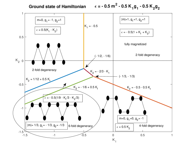
Figure 1: Structure of the ground states in the $(K_{1},K_{2})$ plane. There are $4$ different structures, depending on the values of the parameters $K_{1}$ and $K_{2}$, defined by the values of the order parameters $m$, $g_{1}$ and $g_{2}$. The colored lines divide the regions having ground states with different structure; beside each line there is the equation defining it. For each region the figure shows the values of the order parameters, the corresponding expression of the energy per particle $\epsilon$, and the degeneracy of the ground state. Apart from the fully magnetized (ferromagnetic) state, there are sketches showing the configuration of the partially magnetized (ferrimagnetic) state and of the two paramagnetic ($m=0$) states; the segments linking neighbouring spins are just for visual clarity.

The lines dividing the various regions in the $(K_{1},K_{2})$ plane are lines of first–order phase transitions. A relevant fact is the presence, in a strip of the $(K_{1},K_{2})$ plane, of a ground state only partially magnetized (sometimes such states are called ferrimagnetic, in contrast to the fully magnetized ferromagnetic states). We note the presence of two triple points, at the coordinates $(K_{1},K_{2})=(-1/2,-1/6)$ and $(K_{1},K_{2})=(-1/3,-1/3)$, respectively. At the former there is equality of the energies of the ferromagnetic state, the ferrimagnetic state, and a paramagnetic ($m=0$) state. At the latter the equality is of the energies of still the ferromagnetic and the ferrimagnetic state, but the third state is another paramagnetic state. Figure 1 shows as well the structure of the two different paramagnetic states. As discussed in the following Section, the triple points are present also for a range of positive temperatures.

4 Solution of the model and results for the phase diagram

4.1 Transfer–matrix solution

Let us now consider the solution of the model (1) by means of the transfer matrix method. The partition function can be written as

$$Z=\sum_{\{S_{i}\}}e^{\frac{\beta}{2N}\left(\sum_{i=1}^{N}S_{i}\right)^{2}+\frac{\beta K_{1}}{2}\sum_{i=1}^{N}S_{i}S_{i+1}+\frac{\beta K_{2}}{2}\sum_{i=1}^{N}S_{i}S_{i+2}}\,,$$ (26)

where $\beta=1/T$ and $\sum_{\{S_{i}\}}$ marks a summation over spin states. With the help of the Gaussian identity (6), the partition function of the system may be rewritten as

$$Z=\sqrt{\frac{\beta N}{2\pi}}\int^{+\infty}_{-\infty}dx\,e^{-\frac{\beta N}{2}x^{2}}\sum_{\{S_{i}\}}\prod_{i=0}^{N/2-1}T_{S_{2i+1},S_{2i+2}}^{S_{2i+3},S_{2i+4}}\,,$$ (27)

where

$$T_{S_{1},S_{2}}^{S_{3},S_{4}} = \exp\left\{\frac{\beta x}{2}\left(S_{1}+S_{2}+S_{3}+S_{4}\right)+\frac{\beta K_{1}}{4}\left(S_{1}S_{2}+S_{3}S_{4}\right)\right.$$ (28)

$$+ \frac{\beta K_{1}}{2}S_{2}S_{3}+\left.\frac{\beta K_{2}}{2}\left(S_{1}S_{3}+S_{2}S_{4}\right)\right\}.$$

We recall that we are assuming periodic boundary conditions, and besides we assume $N$ to be even; both assumptions, useful for the computation, are physically irrelevant in the thermodynamic limit. The partition function can be rewritten into the following form

$$Z=\sqrt{\frac{\beta N}{2\pi}}\int^{+\infty}_{-\infty}dx\,e^{-\frac{\beta N}{2}x^{2}}\,\mbox{Tr}\,T^{N/2}\,.$$ (29)

Here $T$ is the transfer matrix which is formed by the elements $T_{S_{1},S_{2}}^{S_{3},S_{4}}$ with on the rows the elements $S_{1}$ and $S_{2}$ and on the columns the elements $S_{3}$ and $S_{4}$ taking values $\pm 1$ (in this Section, and in some expressions of Section 4.2.1, $T$ denotes the transfer matrix rather than the temperature; this should not give rise to confusion). The transfer matrix $T$ reads

$$T=\left(\begin{array}[]{cccc}e^{\beta\left(K_{1}+K_{2}+2x\right)}&e^{\beta\left(\frac{K_{1}}{2}+x\right)}&e^{\beta\left(-\frac{K_{1}}{2}+x\right)}&e^{-\beta K_{2}}\\ e^{\beta\left(-\frac{K_{1}}{2}+x\right)}&e^{\beta\left(-K_{1}+K_{2}\right)}&e^{-\beta K_{2}}&e^{\beta\left(\frac{K_{1}}{2}-x\right)}\\ e^{\beta\left(\frac{K_{1}}{2}+x\right)}&e^{-\beta K_{2}}&e^{\beta\left(-K_{1}+K_{2}\right)}&e^{\beta\left(-\frac{K_{1}}{2}-x\right)}\\ e^{-\beta K_{2}}&e^{\beta\left(-\frac{K_{1}}{2}-x\right)}&e^{\beta\left(\frac{K_{1}}{2}-x\right)}&e^{\beta\left(K_{1}+K_{2}-2x\right)}\end{array}\right).$$ (30)

$\mbox{Tr}T^{N/2}$ in the Eq. (29) means a trace of the matrix $T^{N/2}$ which can be expressed through the eigenvalues of $T$ as

$$\mbox{Tr}T^{N/2}=\lambda_{1}^{N/2}+\lambda_{2}^{N/2}+\lambda_{3}^{N/2}+\lambda_{4}^{N/2}.$$ (31)

The eigenvalues of a nonsymmetric real matrix can be real or complex (appearing in complex conjugate pairs). In our case we can rely on the Perron–Frobenius theorem [31, 32, 33], that assures that for a matrix with strictly positive elements, like our $T$, the eigenvalue with the largest modulus is real and positive. Let us denote with $\lambda(x)$ (writing explicitly its dependence on $x$) this eigenvalue. From Eqs. (29) and (31) it is clear that in the thermodynamic limit the contribution of the other eigenvalues can be neglected. The partition function of the system may be finally written as

$$Z=\sqrt{\frac{\beta N}{2\pi}}\int^{+\infty}_{-\infty}dx\,e^{-N\beta\tilde{f}(\beta,x)}\,,$$ (32)

where

$$\tilde{f}(\beta,x)=\frac{1}{2}x^{2}-\frac{1}{2\beta}\ln\lambda(x)\,.$$ (33)

The integral in Eq. (32) can be performed by the saddle–point method, and in the limit $N\rightarrow\infty$ one obtains the following expression of the free energy per particle

$$f(\beta)=\min_{x}{\Bigg{\{}\frac{1}{2}x^{2}-\frac{1}{2\beta}\ln\lambda(x)\Bigg{\}}}\,.$$ (34)

Although it is possible to write the analytical expression of $\lambda(x)$, since $T$ is a $4\times 4$ matrix, we have preferred to obtain it numerically with the code that is also employed to find the minimum indicated in Eq. (34).

4.2 Phase Diagrams

We are now in the position to discuss the phase diagram of the model. We decided to show the phase diagram in the two–dimensional $(K_{1},T)$ plane for different values of $K_{2}$, which is indeed a convenient way to understand the rich structure of the phase diagram. We preliminarily observe that the two limiting cases $K_{2}\to 0$, in which the long–range term competes with the NN coupling $K_{1}$, and $K_{1}\to 0$, with only long–range and the NNN coupling $K_{2}$, have the same (two–dimensional) phase diagram. Indeed, as discussed in Sections 2.1 and 2.2, the model with $K_{1}=0$ has the same free energy of the model with $K_{2}=0$ and $K_{1}=K_{2}$. This, together with the need to have a visualization of the phase diagram that overall depends on $K_{1}$, $K_{2}$ and $T$, suggests to fix one of two couplings $K_{1}$, $K_{2}$ and vary the other at finite $T$. Since the properties of the $K_{2}=0$ model are very well studied [27, 28, 29], we decided to fix $K_{2}$ and study the phase diagram in the $(K_{1},T)$ plane, analyzing how its structure depends on the chosen fixed value of $K_{2}$.

A very rich structure of the phase diagram, coming from the interplay between the competing interactions and the long–term coupling, emerges. Depending on the values of $K_{2}$, we obtain eight different phase diagrams qualitatively different between them.

In the following we study and show these eight regions separately, and we postpone a qualitative discussion of the obtained findings to Section 5.

4.2.1 Region A: $K_{2}>K_{2}^{a}\simeq-0.0885$

In this region, where $K_{2}$ is larger than a value denoted by $K_{2}^{a}$, with $K_{2}^{a}\simeq-0.0885$, the phase diagram in the $(K_{1},T)$ plane is qualitatively the same of the phase diagram for $K_{2}=0$, meaning that the position of the first–order and second–order transition lines depends explicitly on $K_{2}$, but apart from that the phase diagram has the same form.

Let us first consider what happens at $T=0$. It can be seen from Figure 1 that the system in Region A exhibits a first–order phase transition, by increasing $K_{1}$, from a paramagnetic ($m=0$) state to a ferromagnetic one. By increasing $T$ the first–order phase transition line changes to a second–order line.

The line of second–order transitions in the $(K_{1},T)$ plane for given $K_{2}$ is in general obtained by looking when the second derivative of the function (33) in $x=0$ vanishes. In addition one has to check that $x=0$ is actually the absolute minimum of that function.

The function $\lambda(x)$ is given implicitly by $\det|T(x)-\lambda{\rm I}|=0$, where the solution of largest modulus has to be taken. It can be seen that $T(x)$ is an even function of $x$, and so is $\lambda(x)$. In fact, if after posing $x\to-x$ one first permutes the rows of $T$ according to $(1,2,3,4)\to(4,3,2,1)$ and then makes the same permutation in the columns, one has again $T(x)$. Since the above permutations do not alter the determinant, this shows that $\det|T(-x)-\lambda{\rm I}|=\det|T(x)-\lambda{\rm I}|$ and $\lambda(-x)=\lambda(x)$, as one could have guessed on physical basis. Then, all odd derivatives of $\det|T(x)-\lambda{\rm I}|$ in $x=0$, and consequently of $\lambda(x)$, vanish.

To proceed, we observe that if $F(x,y)=0$ defines implicitly the function $y(x)$, then, using the usual notation for partial derivatives, we have

$$\frac{\mbox{d}y}{\mbox{d}x}\equiv y_{x} = -\frac{F_{x}}{F_{y}}\,,$$ (35)

$$\frac{\mbox{d}^{2}y}{\mbox{d}x^{2}}\equiv y_{xx} = -\frac{F_{xx}+2F_{xy}y_{x}+F_{yy}y_{x}^{2}}{F_{y}}\,.$$ (36)

In our case $F=\det|T(x)-\lambda{\rm I}|$, with $\lambda$ playing the role of $y$. We have seen that $F_{x}=F_{xy}=y_{x}=0$, so that

$$\frac{\mbox{d}^{2}\lambda}{\mbox{d}x^{2}}=-\frac{F_{xx}}{F_{\lambda}}\,.$$ (37)

Let us denote with $T^{(p)}$ the determinant of $T$ after the substitution of the $p$-th column with the derivative of its elements with respect to $x$. For example, in $T^{(1)}$ the first column of $T$ is substituted by $\left[2\beta e^{\beta\left(K_{1}+K_{2}+2x\right)},\beta e^{\beta\left(-\frac{K_{1}}{2}+x\right)},\beta e^{\beta\left(\frac{K_{1}}{2}+x\right)},0\right]^{T}$. In the same way, we denote with $T^{(p,q)}$ the determinant of $T$ after the substitution: ($i$) if $p\neq q$, of the $p$-th column with the derivative of its elements with respect to $x$ and of the $q$-th column with the derivative of its elements with respect to $x$; ($ii$) if $p=q$, of the $p$-th column with the second derivative of its elements with respect to $x$. Then, we have:

$$F_{xx}=\sum_{p=1}^{4}\sum_{q=1}^{4}T^{(p,q)}\,.$$ (38)

Furthermore, we denote with $T_{(p)}$ the determinant of $T$ after the substitution of the $p$-th column with a column with $-1$ in the $p$-th row and $0$ in the other three rows. Then

$$F_{\lambda}=\sum_{p=1}^{4}T_{(p)}\,.$$ (39)

So finally

$$\left.\frac{\mbox{d}^{2}\lambda}{\mbox{d}x^{2}}\right|_{x=0}\equiv\lambda^{(2)}=\left.-\left\{\left[\sum_{p=1}^{4}\sum_{q=1}^{4}T^{(p,q)}\right]\left[\sum_{p=1}^{4}T_{(p)}\right]^{-1}\right\}\right|_{x=0}\,.$$ (40)

For $x\to 0$, we can take $\lambda(x)=\lambda(0)+\frac{1}{2}\lambda^{(2)}x^{2}$, and then $\ln\lambda(x)=\ln\lambda(0)+\frac{1}{2\lambda(0)}\lambda^{(2)}x^{2}$. Then, the second derivative (with respect to $x$) in $x=0$ of the expression in curly brackets in Eq. (34) is given by $1-\lambda^{(2)}/[2\beta\lambda(0)]$. By numerically finding where the latter expression vanishes in the $(K_{1},T)$ plan, one obtains the points potentially belonging to the line of second–order transitions. The points among them that actually belong to the line are those that, in addition, are an absolute minimum of the expression in the brackets in Eq. (34). Therefore, from the operative point of view, to determine the second–order line, the minimum search implied in Eq. (34) has to be performed only for the $(\beta,K_{1})$ values where $1-\lambda^{(2)}/[2\beta\lambda(0)]$ vanishes. Finally, to complete the determination of the phase diagram, one has to determine the locus of points in which the magnetization value has a discontinuity, therefore obtaining the first–order phase transition line.

The corresponding results are plotted in Figure 2 (left) for a value of $K_{2}$ in the region A ($K_{2}=-0.06$). It is seen that when the temperature decreases the second–order line ends at a tricritical point, and that from there a first–order line originates, going up to $T=0$. For the value of $K_{2}$ chosen in Figure 2 (left) the coordinates of the tricritical point are $(K_{1}\backsimeq-0.330,T\backsimeq 0.495$). It has to be observed that the phase diagram plotted in Figure 2 (left) is qualitatively the same as the canonical phase diagram discussed in [28, 29] for $K_{2}=0$.

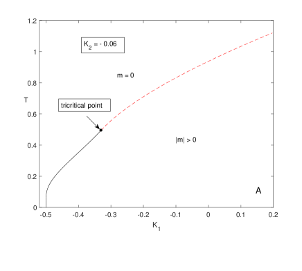
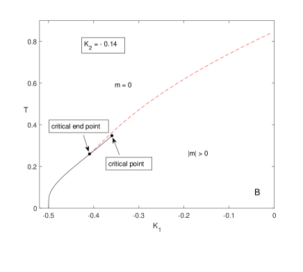
Figure 2: (left)$(K_{1},T)$ phase diagram of the model corresponding to the value $K_{2}=-0.06$ in the region $A$. In this, and in all the other plots of phase diagrams, solid and dashed lines are the first– and second–order phase transition lines, respectively. (right) Phase diagram for $K_{2}=-0.14$ in the region $B$.

4.2.2 Region B: $-0.1542\simeq K_{2}^{b}<K_{2}<K_{2}^{a}\simeq-0.0885$

When the NNN coupling $K_{2}$ is further decreased below the critical value $K_{2}^{a}$, then below the second–order transition line a first–order line emerges. This implies that the second–order line terminates at a critical end point, while the first–order line starting at $T=0$ ends at a critical point. The section of the first–order line between the critical end point and the critical point separates two different magnetized phases (see right panel of Figure 2). As usual in the presence of a critical point ending a first–order transition line, the two phases could be connected by a path in the $(K_{1},T)$ phase diagram that does not intersect the transition line, so that moving on the path one does not encounter discontinuities in the magnetization. This peculiar phase diagram, obtained following the procedure described in Section 4.2.1, occurs when $K_{2}$ is between a value $K_{2}^{b}\simeq-0.1542$ and $K_{2}^{a}$. A typical phase diagram for a value of $K_{2}$ in the region B ($K_{2}=-0.14$) is reported in Figure 2 (right), where the coordinates of the critical end point and of the critical points are respectively $(K_{1}\backsimeq-0.409,T\backsimeq 0.259)$ and $(K_{1}\backsimeq-0.359,T\backsimeq 0.347$).

4.2.3 Region C: $-1/6<K_{2}<K_{2}^{b}\simeq-0.1542$

Below $K_{2}^{b}$, in the region C defined by $-1/6<K_{2}<K_{2}^{b}\simeq-0.1542$, the first–order line bifurcates in a triple point. One of the two first–order line ends at a critical point, as in region B, but the other terminates at a new tricritical point where it meets the second–order line. The phase diagram for the value $K_{2}=-0.16$ in the region C is reported in Figure 3 (left), where the coordinates of the tricritical point, of the triple point and of the critical point are respectively ($K_{1}\backsimeq-0.499,T\backsimeq 0.095$), ($K_{1}\backsimeq-0.493,T\backsimeq 0.076$) and ($K_{1}\backsimeq-0.355,T\backsimeq 0.329$).

To better illustrate the behaviour of thermodynamic quantities in region C, we plot in Figure 4 the magnetization as a function of temperature (left) and the temperature as a function of the energy per particle (right) for the same value of $K_{2}$ chosen in Figure 3, $K_{2}=-0.16$. $K_{1}$ is chosen so that, fixing both $K_{2}$ and $K_{1}$ and increasing $T$ one passes through the first–order line connecting the triple point and the tricritical point. One clearly see in Figure 4 (left) that with $K_{1}=-0.496$, increasing $T$ the magnetization drops down to $0$, it is again different from zero with a jump, and then go smoothly to zero in correspondence of the second–order phase transition. In Figure 4 (right) we have plotted the so–called caloric curve (temperature $T$ vs the energy per particle $\epsilon$), in which the two flat regions show the energy jumps in correspondence of the two first–order phase transitions (Maxwell construction).

4.2.4 Region D: $-0.2672\simeq K_{2}^{c}<K_{2}<-1/6$

The behaviour of region C changes at $K_{2}=-1/6$, as one can understand by looking at the $T=0$ ground state diagram of Figure 1. For $K_{2}>-1/6$, at low temperature for $T\to 0$ there are only two phases: one having magnetization $m=0$ and the other $|m|>0$, and by fixing a small enough $T$ and $K_{2}>-1/6$ one can pass from one region to the other by a first–order transition. The situation changes for $K_{2}<-1/6$, where two first–order lines start from $T=0$. In other words, the triple point of region C occurs at a decreasing temperature when $K_{2}$ decreases, and when it reaches $T=0$ at $K_{2}=-1/6$, then it gives rise to two first–order lines by further decreasing $K_{2}$. It is very interesting to notice that while one of two lines turns right increasing the temperature, i.e. $dT_{c}^{I;a}/dK_{1}>0$, the new first–order line turns left, i.e. $dT_{c}^{I;b}/dK_{1}<0$ (where we denote by $T_{c}^{I;a}$ and $T_{c}^{I;b}$ the two first–order lines, where the ${}^{\prime\prime}a^{\prime\prime}$–one is the one for larger values of $K_{1}$). Furthermore, the second–order line reaches the ${}^{\prime\prime}b^{\prime\prime}$ first–order line in a tricritical point, so that in region D the phase diagram features a critical point and a tricritical point.

A typical phase diagram for a value of $K_{2}$ in the region D ($K_{2}=-0.25$) is reported in Figure 3 (right); the coordinates of the tricritical point and of the critical point are ($K_{1}\backsimeq-0.676,T\backsimeq 0.092$) and ($K_{1}\backsimeq-0.288,T\backsimeq 0.305$), respectively.

The behaviour of the line ${}^{\prime\prime}b^{\prime\prime}$ can be defined re–entrant, in the sense that there is a region of values of $K_{1}$ in which fixing $K_{1}$ and increasing $T$ starting from $T=0$ the system exhibits two phase transitions, in this case one of the first–order from vanishing $m$ to positive $|m|$ and the other of second–order. Re–entrant phase diagrams were discussed and found in Josephson junction arrays [34]. The presence of re–entrance in both models, despite the obvious differences between the quantum phase model describing Josephson networks and the classical $J$-$K_{1}$-$K_{2}$ model studied here, traces back its common element in the presence of NNN terms in the respective Hamiltonians. Indeed, if the interaction term is diagonal in the quantum phase model, there is apparently no re–entrance, as one can see by mean–field and self–consistent harmonic approximations [34, 35, 36, 37]. At variance, if there is a non–diagonal capacitance matrix, giving rise to nonlocal terms, including a NNN coupling, then re–entrance occurs, as confirmed by Monte Carlo simulations [38].

We will see that the other regions E-H similarly display re–entrant behaviours.

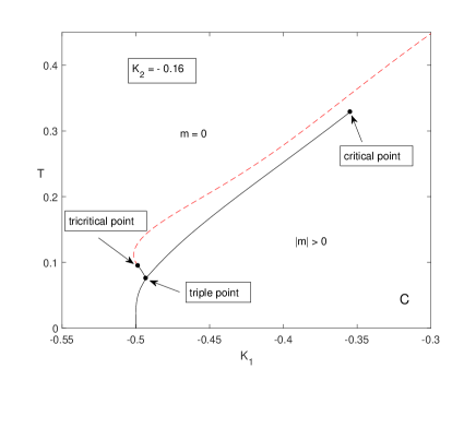
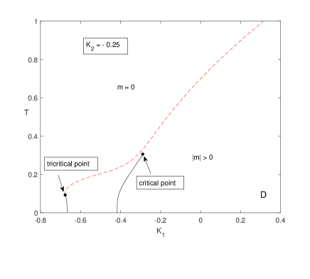
Figure 3: (left)$(K_{1},T)$ phase diagram for $K_{2}=-0.16$ in the region $C$. (right) Phase diagram for $K_{2}=-0.25$ in the region $D$.

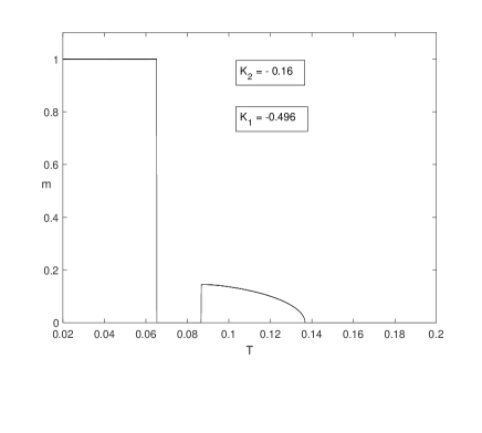
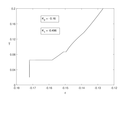
Figure 4: (left) Magnetization vs temperature for $K_{1}=-0.496$ and $K_{2}=-0.16$ in region C. (right) Temperature vs energy per particle (caloric curve) for the same value of the parameters. The two flat regions are the Maxwell constructions in correspondence of the two first–order phase transitions; the discontinuity of the derivative in correspondence of the second–order phase transition at $\epsilon\backsimeq-0.139$ and $T\backsimeq 0.137$ is hardly visible.

4.2.5 Region E: $-0.2745\simeq K_{2}^{d}<K_{2}<K_{2}^{c}\simeq-0.2672$

When the critical value $K_{2}^{c}\simeq-0.2672$ is reached, further increasing $K_{2}$ in modulus the second–order line seen in region $D$ breaks in two pieces: in fact, a first–order line, limited by two tricritical points, appears; this line is denoted by ${}^{\prime\prime}c^{\prime\prime}$ in the following. So in total one has three first–order lines; the other two, ${}^{\prime\prime}a^{\prime\prime}$ and ${}^{\prime\prime}b^{\prime\prime}$, the leftmost of which again showing re–entrant behaviour, are qualitatively as in Region D.

The phase diagram for the value $K_{2}=-0.27$ in the region E is plotted in Figure 5 (left), where the coordinates of the three tricritical points are $(K_{1}\backsimeq-0.715,T\backsimeq 0.091)$, ($K_{1}\backsimeq-0.238,T\backsimeq 0.355$) and ($K_{1}\backsimeq-0.175,T\backsimeq 0.446$), while the critical point is at $(K_{1}\backsimeq-0.259,T\backsimeq 0.318)$. Note that in Figure 5 (left) the critical point is very close, but not on, the second–order order line connecting the two tricritical points having the smaller temperatures.

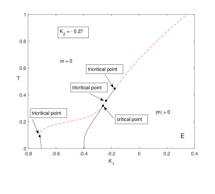
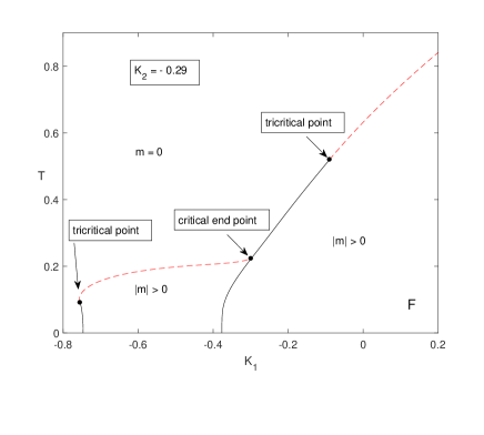
Figure 5: Phase diagram for $K_{2}=-0.27$ in the region $E$ (left) and for $K_{2}=-0.29$ in the region $F$ (right). In the left figure the critical point is very close, but not on, the second–order order line connecting two tricritical points.

4.2.6 Region F: $-0.2953\simeq K_{2}^{e}<K_{2}<K_{2}^{d}\simeq-0.2745$

In region E, increasing the $K_{2}$ in modulus, the length of the first–order line ${}^{\prime\prime}c^{\prime\prime}$ (as denoted in 4.2.5) between the two tricritical points with higher temperatures, and connected to the two second–order lines, increases. When the value $K_{2}^{d}\simeq-0.2745$ is reached, this first–order line ${}^{\prime\prime}c^{\prime\prime}$ merges with the first–order line ${}^{\prime\prime}a^{\prime\prime}$ introduced in region D and present as well in region E. Therefore a second–order line connects the re-entrant line ${}^{\prime\prime}b^{\prime\prime}$ to this merged first–order line, with the latter ending in a tricritical point and featuring a critical end point. In Figure 5 (right), the phase diagram for the value $K_{2}=-0.29$ in the region F is reported. The coordinates of the two tricritical points are $(K_{1}\backsimeq-0.755,T\backsimeq 0.091)$ and ($K_{1}\backsimeq-0.090,T\backsimeq 0.520$), while the critical end point is $(K_{1}\backsimeq-0.299,T\backsimeq 0.223)$.

4.2.7 Region G: $-1/3<K_{2}<K_{2}^{e}\simeq-0.2953$

Passing from region B to region C, a first–order line bifurcates and a triple point emerges. The same happens when the value $K_{2}^{e}\simeq-0.2953$ is reached, entering the region G. In such a region the line ${}^{\prime\prime}a^{\prime\prime}$ bifurcates in a triple point, and two first–order lines starts from there, ending at two tricritical points that separates them from two second–order lines. Interestingly, below the triple point the first–order line separates two regions with non vanishing magnetization.

The phase diagram for the value $K_{2}=-0.31$ in the region G is plotted in Figure 6 (left), where the triple point is $(K_{1}\backsimeq-0.325,T\backsimeq 0.146)$, while the three tricritical points are at $(K_{1}\backsimeq-0.795,T\backsimeq 0.091)$, $(K_{1}\backsimeq-0.354,T\backsimeq 0.167)$ and $(K_{1}\backsimeq-0.023,T\backsimeq 0.564)$.

4.2.8 Region H: $K_{2}<-1/3$

When the value of $K_{2}$ reaches $K_{2}=-1/3$, the first–order line ${}^{\prime\prime}a^{\prime\prime}$ does not any longer separate two regions with non vanishing magnetization, but actually the region with zero magnetization persists at very low temperature arriving to $T=0$ (region H). This part of the phase diagram is surrounded by two first–order lines ending in tricritical points, from which two second–order lines depart. The leftmost of them reaches at a tricritical point the third, pre–existing, first–order line. As one can see in Figure 6 (right), therefore a “lobe” with non vanishing magnetization forms in the zero magnetization. This lobe features two first–order lines ending in two tricritical points, separated by a second–order line. Moreover, the line with a tricritical point separating a first–order and a second–order line, as seen in region A, is present for larger values of $K_{1}$.

Figure 6 (right) shows the phase diagram for the value of $K_{2}=-0.35$ in the region H, where the three tricritical points are at ($K_{1}\backsimeq-0.875,T\backsimeq 0.091)$, $(K_{1}\backsimeq-0.449,T\backsimeq 0.144)$ and $(K_{1}\backsimeq 0.101,T\backsimeq 0.631$).

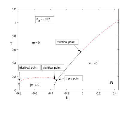
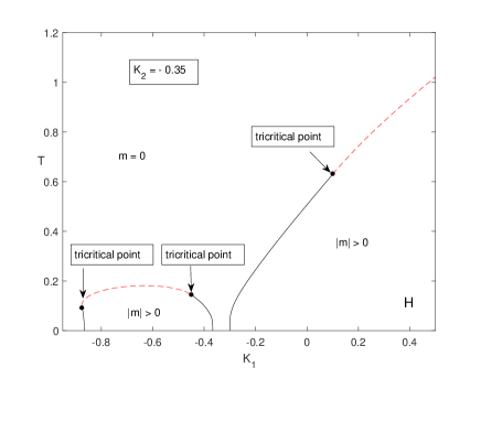
Figure 6: Phase diagram for $K_{2}=-0.31$ in the region $G$ (left) and for $K_{2}=-0.35$ in the region $H$.

Further decreasing $K_{2}$ one has that the lobe moves towards left, but apart from that no qualitative changes in the phase diagram are expected. Notice that when both $K_{1}$ and $K_{2}$ becomes large in modulus, this corresponds to have $J$ going to zero (since we are putting $J=1$), and in this limit the transition occurs only at lower and lower temperatures. A similar situation occurs for $K_{1}$ and $K_{2}$ positive and large, so that we expect that in region A no qualitative changes occurs increasing, e.g., $K_{2}$.

Finally, we observe that if one fixes $K_{1}$ and look at the phase diagrams in the $(K_{2},T)$ plane, one expects to find again the same singularities; we defer a discussion on this point to the next Section.

5 Discussion

The classification of phase transitions in systems with long–range interactions [39] shows that the structure of phase diagrams can be quite complex. The model studied in this work provides a concrete example of this fact. The Hamiltonian has two parameters, $K_{1}$ and $K_{2}$, and therefore the phase diagram lies in the three–dimensional space $(K_{1},K_{2},T)$. We have chosen to plot two–dimensional cuts of the phase diagram, defined by different fixed values of $K_{2}$. This was due to the usefulness to have a simple visualization of the diagram, but at the same time this provided a comparison with the rather simple two–dimensional phase diagram of the model with only the NN coupling $K_{1}$ (i.e., with $K_{2}=0$). The complexity of the phase diagram has resulted in a quite rich behaviour of these two–dimensional plots. In fact, eight qualitatively different structures of two–dimensional phase diagrams are present, each one with its own structure of first– and second–order phase transition lines and points that in the plots occur in four different types: tricritical points, triple points, critical end points, and critical points. For brevity, in this discussion we refer collectively to these four types of points as relevant points.

Each one of the eight different structures occurs for a given range of $K_{2}$, and in the previous Section we have shown a diagram for each structure. In the following we provide a qualitative description of the changes occurring when moving from one structure to another in terms of the change in the occurrence of relevant points. Afterwards, we will give a more general view based on the classification of singularities that can be present in the phase diagrams [39]. The passages are indicated in the following list.

• A tricritical point splitting in a pair consisting of a critical end point and a critical point. This is seen passing through the value of $K_{2}$ given by $K_{2}=K_{2}^{a}\simeq-0.0885$, i.e. passing from region A to region B, see the two panels of Figure 2.

• A critical end point splitting in a pair consisting of a triple point and a tricritical point. This is seen at the value $K_{2}=K_{2}^{b}\simeq-0.1542$, passing from region B to region C, as seen in Figures 2 (right) and 3 (left), and at the value $K_{2}=K_{2}^{e}\simeq-0.2953$, passing from region F to region G, see Figures 5 (right) and 6 (left).

• A triple point reaching $T=0$ and giving rise to a pair of first–order lines starting at $T=0$, and separated (at $T=0$) by a region in which the magnetization is not vanishing. This is seen from region C to region D, at $K_{2}=-1/6$, see the two panels of Figure 3. Also at $K_{2}=-1/3$, as illustrated in the comparison of the two panels of Figure 6, showing the passage from region G to region H, there is an increase, in this case from $2$ to $3$, of the number of first–order lines starting from $T=0$.

• A first–order line, between two emerging tricritical points, generated in a second–order line. This is seen in Figures 3 (right) and 5 (left), with the passage from region D to region E occurring at $K_{2}=K_{2}^{c}\simeq-0.2672$.

• A pair consisting of a tricritical point and a critical point merging in a critical end point. This is seen passing from region E to region F, at $K_{2}=K_{2}^{d}\simeq-0.2745$, as one can notice in the two panels of Figure 5.

5.1 Classification of singularities

If the Hamiltonian of a model has $p$ parameters (in our case $p=2$), its thermodynamic phase diagram has $p+1$ dimensions, corresponding to the parameters plus the temperature $T$. In the phase diagram there can be singularities that span hypersurfaces of dimension $0$ (points), $1$ (lines), $2$ (surfaces), and so on up to $p$; therefore in our case we can have singularities spanning points, lines and surfaces in a three–dimensional space. A singularity is said to be of codimension $n$ if it spans a hypersurface of dimension $p-n$; thus here we have singularities of codimension $0$ (surfaces), $1$ (lines) and $2$ (points). In Ref. [39] a complete classification of codimension–$0$ and codimension–$1$ singularities, in systems with long–range interactions, has been given. Our results can be discussed in that framework.

Clearly the first– and second–order phase transition lines of our two–dimensional plots correspond to surfaces in the three–dimensional $(K_{1},K_{2},T)$ space and are codimension–$0$ singularities, while the relevant points in our plots correspond to lines in the $(K_{1},K_{2},T)$ space and are codimension–$1$ singularities. Furthermore, the codimension–$1$ lines result from the intersection of two codimension–$0$ surfaces. It is then not difficult to see that codimension–$2$ singularities are the points resulting from the intersection of three surfaces, and in fact in a three–dimensional space three surfaces generically (i.e., apart from particular cases) meet in a point. Such a point can also be seen as the point where the three lines defined by the intersection of the three couples of surfaces, formed out of the three surfaces, converge. It must be stressed that each one of the three lines converge to the point only from one direction, since beyond the point each line would correspond to non–equilibrium (unstable or metastable) states.

In this respect, the meeting and splitting of relevant points described in the list above, is the description of the convergence of codimension–$1$ singularities (lines) in a codimension–$2$ singularity (point) (with an exception that we treat below). In order for a codimension–$2$ singularity to appear in one of our two–dimensional plots at fixed $K_{2}$, we should have made the plot for exactly the $K_{2}$ value where the singularity occurs, and the $K_{2}$ values of these singularities are the range boundaries that we have specified in the previous section and in the list above. On the basis of these arguments, one can argue the following. Had we chosen another way to present our results in two–dimensional plots, e.g., by plotting $(K_{2},T)$ diagrams at various fixed values of $K_{1}$, or by choosing other more complicated two–dimensional cuts defined by various fixed values of the quantity $aK_{1}+bK_{2}$ with given $a$ and $b$, we still would have observed a qualitative change of structure at the passage of the plane through the $(K_{1},K_{2},T)$ points where the codimension–$2$ singularities are located. However, this qualitative changes would have been characterized, in general, by meetings and splittings of relevant points different from those given in the list above. The conclusion is that apart from the last details, we would have observed the same sequence of qualitative change of structures, and the same richness of such structures, for any choice of two–dimensional cuts of the phase diagram. We observe that the appearance of two tricritical points (the passage from region D to region E) is not due to the crossing of a codimension–$2$ singularities, but it is the result of the following fact. In region E the plane with constant $K_{2}$ crosses the line of tricritical points in two distinct points of the $(K_{1},T)$ plane; approaching the boundary with region D the two points approach each other, until at $K_{2}=K_{2}^{c}$ the plane is tangent to the line of tricritical points and the two points in the $(K_{1},T)$ plane coincide. When $K_{2}$ enters the range of region D there is no more an intersection, and there are no more tricritical points in the $(K_{1},T)$ plane. Although this qualitative change is not related to a codimension–$2$ singularity, it still would manifest itself in another choice of two–dimensional cuts, since the same mechanism would occur.

It is clear that adding couplings acting at larger distances, such $K_{3}$, $K_{4}$ and so on, the phase diagram would have further dimensions and would become very complex. For example, with just the presence of $K_{3}$ the phase diagram would be four–dimensional, and one could, e.g., represent it with three–dimensional cuts at various fixed values of $K_{3}$. From the results presented in this work one can guess that the number of qualitatively different structures of such three–dimensional plots, varying $K_{3}$, would be quite large, and the passage from one structure to the others, due to the crossing of codimension–$3$ singularities, would be characterized by an extremely rich set of possibilities. This shows that this class of systems with finite–range coupling in presence of a long–range term appears to be an ideal playground to see in simple, yet meaningful, models, the behaviour of thermodynamical singularities and the relation between different types of critical points.

6 Conclusions

In this paper we studied an Ising spin chain with short–range competing interactions in presence of long–range couplings. We worked out the partition function of the model and the phase diagram in the canonical ensemble. We found that eight possible, qualitatively different two–dimensional phase diagrams exist in the parameter space. They occur as a result of the frustration and the competition between the short– and the long–range interactions.

One of the motivations of our work was that, when one of the two short–range interactions is turned off, the system exhibits ensemble inequivalence and the thermodynamic and dynamical behavior of the system in both the canonical and microcanonical ensembles may be different. Our study is a first step in the investigation of the effects of additional finite–range coupling terms, since we provided a full characterization of the canonical phase diagrams. Therefore, it is appealing to consider the solution of the model studied in this paper in the microcanonical ensemble. For such a study one could apply the method of determining the entropy presented in Ref. [40]. One can anticipate that a very rich microcanonical behaviour occurs when $K_{2}$ is added. This can be argued from the fact that with $K_{2}=0$ the canonical phase diagram has only a tricritical point, while for $K_{2}\neq 0$ one has all the possibilities described in Section 4. It would be then very interesting to work out the details of the comparison between the two ensembles, and study their inequivalence when $K_{2}$ is turned on.

Several extensions of the model studied here could be as well very interesting. One could study, in the same one–dimensional geometry considered in the present paper: i) the effect of short–range interactions in presence of mean-field terms for $O(n)$ models [41, 42, 43], ii) spin–$1$ systems [44], iii) more general long–range interactions with power–law decay [26], and iv) the effect of a short–range term in the Sherrington-Kirkpatrick spin glass model [1]. It would be also appealing to consider our model in higher dimensions, since it is known that already in two dimensions one can have antiferromagnetic phases at finite temperature [45]. One could also ask whether it is possible to enlarge the re–entrance in the phase diagram by having short–range terms involving more couplings. Finally, it would be very deserving to study the quantum version of the classical model considered here and compare the results with other quantum models with competing short– and long–range interactions [46].

Appendix A The evaluation of the ground state

For convenience we reproduce here the expressions of the energy per particle and the allowed ranges of the order parameters:

$$\epsilon=-\frac{1}{2}\left(m^{2}+K_{1}g_{1}+K_{2}g_{2}\right)\,,$$ (41)

$$\mkern-36.0mu\mkern-36.0mu-1\leq m\leq 1,\,\,\,\,\,\,\,\,\,2|m|-1\leq g_{1}\leq 1,\,\,\,\,\,\,\,\,\,\max(2|m|-1,2|g_{1}|-1)\leq g_{2}\leq 1\,.$$ (42)

The evaluation of the order parameter values giving the ground state can be divided in four steps, corresponding respectively to the four quadrants of the $(K_{1},K_{2})$ plane.

I) $K_{1}\geq 0$, $K_{2}\geq 0$

The state of lowest energy is obtained when all three order parameters are equal to $1$, i.e., with a fully magnetized system.

II) $K_{1}<0$, $K_{2}\geq 0$

For given $m$ and $g_{1}$ the lowest energy is achieved for $g_{2}=1$, giving

$$\epsilon=-\frac{1}{2}\left(m^{2}+K_{1}g_{1}+K_{2}\right)\,.$$ (43)

Since $K_{1}$ is negative, for given $m$ the lowest value of this expression is obtained for the smallest allowed value of $g_{1}$. This value, restricting to $m\geq 0$ (as we have explained can be done), is $2m-1$. Then we have to find the smallest value of

$$\epsilon=-\frac{1}{2}\left(m^{2}+2K_{1}m-K_{1}+K_{2}\right)$$ (44)

for $0\leq m\leq 1$. One finds right away that this is obtained for $m=1$ (and thus $g_{1}=1$) for $K_{1}>-\frac{1}{2}$, and for $m=0$ (and thus $g_{1}=-1$) for $K_{1}<-\frac{1}{2}$.

III) $K_{1}\geq 0$, $K_{2}<0$

The two cases with $K_{2}<0$ are less immediate. When $K_{1}\geq 0$ we can proceed as follows. From the inequalities (42) one deduces that $g_{1}\leq(1+g_{2})/2$. Then, since $K_{1}\geq 0$, for given $m$ and $g_{2}$ the lowest value of the energy per particle (41) is obtained for $g_{1}=(1+g_{2})/2$, giving

$$\epsilon=-\frac{1}{2}\left[m^{2}+\left(\frac{1}{2}K_{1}+K_{2}\right)g_{2}+\frac{1}{2}K_{1}\right]\,.$$ (45)

If $\frac{1}{2}K_{1}+K_{2}>0$ the minimum of this expression is obtained for $g_{2}=1$ (and thus $g_{1}=1$) and $m=1$. If $\frac{1}{2}K_{1}+K_{2}<0$ the minimum for given $m$ is achieved for $g_{2}=2m-1$ (and thus $g_{1}=m$), to have

$$\epsilon=-\frac{1}{2}\left[m^{2}+\left(K_{1}+2K_{2}\right)m-K_{2}\right]\,.$$ (46)

The minimum of this expression (for $0\leq m\leq 1$) occurs for $m=0$ (and thus $g_{2}=-1$ and $g_{1}=0$) when $K_{2}<-\frac{1}{2}K_{1}-\frac{1}{2}$, and for $m=1$ (and thus $g_{2}=1$ and $g_{1}=1$) when $K_{2}<-\frac{1}{2}K_{1}-\frac{1}{2}$. Considering also the situation in which $\frac{1}{2}K_{1}+K_{2}>0$, the last two expression give the overall result for this case ($K_{1}\geq 0$ and $K_{2}<0$).

IV) $K_{1}<0$, $K_{2}<0$

This is the case requiring more attention. It is convenient to divide the range $0\leq m\leq 1$ in the two subranges $0\leq m\leq 1/3$ and $1/3\leq m\leq 1$. Let us begin with the latter.

$a$) $1/3\leq m\leq 1$. The smallest allowed value of $g_{1}$, i.e., $2m-1$, can be negative if $m<1/2$. However, regardless of this possibility, for $m\geq 1/3$ it will always be $-(2m-1)\leq m$; therefore, for $2m-1\leq g_{1}\leq m$ it will always be $m\geq|g_{1}|$. Consequently, for given $m$ in this subrange and given $g_{1}$ between $2m-1$ and $m$, the lowest value of the energy (41) is obtained for $g_{2}=2m-1$. On the other hand, when $m\leq g_{1}\leq 1$ the lowest value occurs for $g_{2}=2g_{1}-1$. After making these positions and seeking for the lowest value varying $g_{1}$, this will occur for $g_{1}=2m-1$, and thus also $g_{2}=2m-1$. We then obtain the expression

$$\epsilon=-\frac{1}{2}\left[m^{2}+2\left(K_{1}+K_{2}\right)m-K_{1}-K_{2}\right]\,.$$ (47)

The minimum of this expression in the range $1/3\leq m\leq 1$ is obtained for $m=1$ (and thus $g_{1}=1$ and $g_{2}=1$) when $K_{2}>-K_{1}-\frac{2}{3}$, and for $m=1/3$ (and thus for $g_{1}=-1/3$ and $g_{2}=-1/3$) when $K_{2}<-K_{1}-\frac{2}{3}$ (reminding that these bounds have to be considered together with $K_{2}<0$). The corresponding minima will have to be compared with the minima in the range $0\leq m\leq 1/3$, to find the overall minima in $m$.

$b$) $0\leq m\leq 1/3$. Now $-(2m-1)$ is larger than $m$. Therefore, we can repeat the above analysis only for $-m\leq g_{1}\leq 1$. As a consequence, the lowest value of the energy for given $m$ in this subrange and for given $g_{1}$ larger than $-m$ is obtained for $g_{1}=-m$ and $g_{2}=2m-1$, giving the expression

$$\epsilon=-\frac{1}{2}\left[m^{2}-\left(K_{1}-2K_{2}\right)m-K_{2}\right]\,.$$ (48)

For $2m-1\leq g_{1}\leq-m$, $|g_{1}|$ is larger than $m$, then the minimum occurs for $g_{2}=2|g_{1}|-1=-2g_{1}-1$. Then

$$\epsilon=-\frac{1}{2}\left[m^{2}+\left(K_{1}-2K_{2}\right)g_{1}-K_{2}\right]\,.$$ (49)

For $K_{1}-2K_{2}>0$ the minimum in $g_{1}$ occurs for $g_{1}=-m$ (and thus $g_{2}=2m-1$), while for $K_{1}-2K_{2}<0$ the minimum in $g_{1}$ occurs for $g_{1}=2m-1$ (and thus $g_{2}=-4m+1$). We then obtain the expressions:

$$\epsilon = -\frac{1}{2}\left[m^{2}-\left(K_{1}-2K_{2}\right)m-K_{2}\right];\,\,\,\,\,\,\,\,\,\,\,\,\,\,\,K_{1}-2K_{2}>0$$ (50)

$$\epsilon = -\frac{1}{2}\left[m^{2}+2\left(K_{1}-2K_{2}\right)m-K_{1}+K_{2}\right];\,\,\,\,\,\,\,\,\,\,\,\,\,\,\,K_{1}-2K_{2}<0$$ (51)

Studying these expressions in the range $0\leq m\leq 1/3$ one finds the minimum occurs for $m=0$, $g_{1}=0$ and $g_{2}=-1$ for $K_{2}<\frac{1}{2}K_{1}-\frac{1}{6}$; it is found for $m=1/3$, $g_{1}=-1/3$ and $g_{2}=-1/3$ for $\frac{1}{2}K_{1}-\frac{1}{6}<K_{2}<\frac{1}{2}K_{1}+\frac{1}{12}$; it occurs for $m=0$, $g_{1}=-1$ and $g_{2}=1$ for $K_{2}>\frac{1}{2}K_{1}+\frac{1}{12}$ (again, all these bounds have to be considered together with $K_{2}<0$).

Comparing the subcases $a$) and $b$) we obtain the configurations with lowest energy in the case IV, i.e., in the quadrant $K_{1}<0$, $K_{2}<0$. We find the following results. For $-\frac{1}{3}\leq K_{1}\leq 0$ the minimum is at $m=1$, $g_{1}=1$ and $g_{2}=1$ for $K_{2}>-\frac{1}{2}K_{1}-\frac{1}{2}$, and at $m=0$, $g_{1}=0$ and $g_{2}=-1$ for $K_{2}<-\frac{1}{2}K_{1}-\frac{1}{2}$. For $-\frac{1}{2}\leq K_{1}\leq-\frac{1}{3}$ the minimum is at $m=0$, $g_{1}=0$ and $g_{2}=-1$ for $K_{2}<\frac{1}{2}K_{1}-\frac{1}{6}$, at $m=1/3$, $g_{1}=-1/3$ and $g_{2}=-1/3$ for $\frac{1}{2}K_{1}-\frac{1}{6}<K_{2}<-K_{1}-\frac{2}{3}$, and at $m=1$, $g=1$ and $g_{2}=1$ for $K_{2}>-K_{1}-\frac{2}{3}$. For $K_{1}\leq-\frac{1}{2}$ the minimum is at $m=0$, $g_{1}=0$ and $g_{2}=-1$ for $K_{2}<\frac{1}{2}K_{1}-\frac{1}{6}$, at $m=1/3$, $g_{1}=-1/3$ and $g_{2}=-1/3$ for $\frac{1}{2}K_{1}-\frac{1}{6}<K_{2}<\frac{1}{2}K_{1}+\frac{1}{12}$, and at $m=0$, $g_{1}=-1$ and $g_{2}=1$ for $K_{2}>\frac{1}{2}K_{1}+\frac{1}{12}$.

At the end, unifying all the cases from I to IV, one obtains, for the ground state, the results described in Section 3 and shown in Figure 1.

References

References

- [1] M. Mezard, G. Parisi, and M. A. Virasoro, Spin glass theory and beyond (Singapore, World Scientific, 1987).
- [2] P. M. Chaikin and T. C. Lubensky, Principles of condensed matter physics (Cambridge, Cambridge University Press, 1995).
- [3] M. Seul and D. Andelman, Science 267, 476 (1995).
- [4] A. Giuliani, J. L. Lebowitz, and E. H. Lieb, AIP Conference Proceedings 1091, 44 (2009).
- [5] S. Chakrabarty and Z. Nussinov, Phys. Rev. B 84, 144402 (2011).
- [6] H. T. Diep, Frustrated spin systems (Singapore, World Scientific, 2004).
- [7] S. Redner, J. Stat. Phys. 25, 15 (1981).
- [8] F. Mila, D. Poilblanc, and C. Bruder, Phys. Rev. B 43, 7891 (1991).
- [9] R. R. P. Singh, W. H. Zheng, C. J. Hamer, and J. Oitmaa, Phys. Rev B 60, 7278 (1999).
- [10] L. Capriotti, F. Becca, A. Parola, and S. Sorella, Phys. Rev. Lett. 87, 097201 (2001).
- [11] J. Sirker, Z. Weihong, O. P. Sushkov, and J. Oitmaa, Phys. Rev. B 73, 184420 (2006).
- [12] M. Spenke and S. Guertler, Phys. Rev. B 86, 054440 (2012).
- [13] L. Wang and A. W. Sandvik, Phys. Rev. Lett. 121, 107202 (2018).
- [14] F. J. Dyson, Comm. Math. Phys. 12, 91 (1969).
- [15] D. J. Thouless, Phys. Rev. 187, 732 (1969).
- [16] J. Sak, Phys. Rev. B 8, 281 (1973).
- [17] E. Luijten and H. W. J. Blöte, Phys. Rev. Lett. 89, 025703 (2002).
- [18] T. Blanchard, M. Picco, and M. A. Rajabpour, Europhys. Lett. 101, 56003 (2013).
- [19] E. Brezin, G. Parisi, and F. Ricci-Tersenghi, J. Stat. Phys. 157, 855 (2014).
- [20] M. C. Angelini, G. Parisi, and F. Ricci-Tersenghi, Phys. Rev. E 89, 062120 (2014).
- [21] N. Defenu, A. Trombettoni, and A. Codello, Phys. Rev. E 92, 052113 (2015).
- [22] N. Defenu, A. Trombettoni, and S. Ruffo, Phys. Rev. B 94, 224411 (2016); Phys. Rev. B 96, 104432 (2017)
- [23] G. Gori, M. Michelangeli, N. Defenu, and A. Trombettoni, Phys. Rev. E 96, 012108 (2017).
- [24] C. Behan, L. Rastelli, S. Rychkov, and B. Zan, Phys. Rev. Lett. 118, 241601 (2017); J. Phys. A 50, 354002 (2017).
- [25] T. Horita, H. Suwa, and S. Todo, Phys. Rev. E 95, 012143 (2017).
- [26] A. Campa, T. Dauxois, D. Fanelli and S. Ruffo, Physics of long-range interacting systems (Oxford, Oxford University Press, 2014).
- [27] J. F. Nagle, Phys. Rev. A 2, 2124 (1970).
- [28] M. Kardar, Phys. Rev. B 28, 244 (1983).
- [29] D. Mukamel, S. Ruffo, and N. Schreiber, Phys. Rev. Lett. 95, 240604 (2005).
- [30] G. Parisi, Statistical field theory (Redwood City, Addison-Wesley, 1988).
- [31] O. Perron, Mathematische Annalen 64, 248 (1907).
- [32] F. G. Frobenius, Sitzungsber. Königl. Preuss. Akad. Wiss. 456 (1912).
- [33] R. S. Varga, Matrix Iterative Analysis, Springer Series in Computational Mathematics, Vol. 27 (Springer, Berlin & Heidelberg, 2009).
- [34] R. Fazio and H. Van Der Zant, Phys. Rep. 355, 235 (2000).
- [35] G. Grignani, A. Mattoni, P. Sodano, and A. Trombettoni, Phys. Rev. B 61, 11676 (2000).
- [36] E. S̆imánek, Inhomogeneous superconductors: granular and quantum effects (Oxford University Press, Oxford, 1994).
- [37] A. Smerzi, P. Sodano, and A. Trombettoni, J. Phys. B 37, S265 (2004).
- [38] L. Capriotti, A. Cuccoli, A. Fubini, V. Tognetti, and R. Vaia, Phys. Rev. Lett. 91, 247004 (2003).
- [39] F. Bouchet and J. Barré, J. Stat. Phys. 118, 1073 (2005).
- [40] G. Gori and A. Trombettoni, J. Stat. Mech. P10021 (2011).
- [41] A. Campa, A. Giansanti, and D. Moroni, J. Phys. A 36, 6897 (2001).
- [42] A. Campa, A. Giansanti, D. Mukamel, and S. Ruffo, Physica A 365, 177 (2006).
- [43] T. Dauxois, P. de Buyl, L. Lori, and S. Ruffo, J. Stat. Mech. P06015 (2010).
- [44] V. V. Hovhannisyan, N. S. Ananikian, A. Campa, and S. Ruffo, Phys. Rev. E 96, 062103 (2017).
- [45] M. Kardar, Phys. Rev. Lett. 51, 523 (1983).
- [46] F. Iglói, B. Blaß, G. Roósz, and H. Rieger, Phys. Rev. B 98, 184415 (2018).