Abstract

We introduce warm quintessential inflation and study it in the weak dissipative regime. We consider the original quintessential inflation model, which approximates quartic chaotic inflation at early times and thawing quartic inverse-power-law quintessence at present. We find that the model successfully accounts for both inflation and dark energy observations, while it naturally reheats the Universe, thereby overcoming a major problem of quintessential inflation model-building.

1 Introduction

Inflation is overwhelmingly the best mechanism for explaining the observed structure in the Universe as well as its spatial flatness and large-scale homogeneity [1]. In the same time, the discovery of dark energy [2] is best attributed to a non-zero, albeit incredibly fine-tuned, cosmological constant in the benchmark paradigm of $\Lambda$CDM [3]. However, recently both proposals have been challenged by the swampland conjectures [4], which stipulate the impossibility of de-Sitter vacua in string theory and also set stringent constraints on inflation model-building and undermine $\Lambda$CDM [5] (but see also Ref. [6]). Such constraints are not possible to meet with conventional inflation [7]. A successful way to model inflation while satisfying the swampland conjectures is incorporating dissipating effects [8], as in warm inflation [9]. On the dark energy front, the observations of the current accelerated expansion can be explained by quintessence instead of a non-zero cosmological constant $\Lambda$ [10], which is also in agreement with the swampland conjectures [11]. In this letter, we attempt to join the two and introduce warm quintessential inflation (for a reference list on quintessential inflation see Refs. [12, 13]), which has the additional advantage of providing a natural mechanism for reheating the Universe. Reheating is of particular significance in quintessential inflation because the conventional reheating by the decay of the inflaton field at the end of inflation cannot occur as the field needs to survive until the present and become quintessence. We use natural units where $c=\hbar=k_{\rm B}=1$ and $8\pi G=m_{P}^{-2}$, where $m_{P}=2.43\times 10^{18}\,$GeV is the reduced Planck mass.

2 The model

The original quintessential inflation model is [14]

$$V(\phi)=\left\{\begin{array}[]{ll}\lambda(\phi^{4}+M^{4})&{\rm for}\quad\phi<0\\ \frac{\mbox{\normalsize$\lambda M^{8}$}}{\mbox{\normalsize$\phi^{4}+M^{4}$}}&{\rm for}\quad\phi>0\end{array}\right.\,,$$ (1)

where $0<M\ll m_{P}$. For negative values of the inflaton field $\phi\ll-M$, the above potential reduces to quartic chaotic inflation, which has been excluded by observations unless it is “warmed up”, by considering significant dissipation effects. During inflation $\phi\sim-m_{P}$. For positive values of the field $\phi\gg M$ the potential becomes inverse power-law (IPL) quintessence. Such quintessence models feature a tracker solution, which however, is too steep to satisfy observations in the case of an inverse quartic potential $V\propto\phi^{-4}$. However, in our case, the field does not follow the tracker but, after the end of inflation, it rushes down its runaway potential and freezes at a value $\phi_{F}\sim m_{P}$ with some residual potential density, which explains dark energy. At present, the field unfreezes and begins slowly rolling down its potential. Such quintessence is called “thawing” [16].

While the field runs from inflation at $\phi\sim-m_{P}$ to quintessence at $\phi\sim m_{P}$ it is kinetically dominated and oblivious of the potential [17]. Thus, the awkward discontinuity (in the fourth derivative) of the potential in Eq. (1) is not felt. In fact, the potential in Eq. (1) is only experienced by the field when $|\phi|\sim m_{P}$, which means that Eq. (1) is only a guideline to the actual form of $V(\phi)$ and should not be taken too seriously.

In addition, the field runs over super-Planckian distance from the end of inflation to its eventual freezing. It is likely that the dissipative properties of the field are different in these two different patches of the scalar potential, which are several Planck scales apart. Indeed, we assume that dissipative effects are important only when the field is slow-rolling during inflation with $\phi\sim-m_{P}$. Additionally, we consider only the weak dissipative regime, where the dynamics of the field are not affected by dissipation (no extra friction) so this issue is not of our concern.

In the weak dissipative regime, the only effect of dissipation is that the quantum fluctuations of the inflaton field during inflation are superseded by its thermal fluctuations, due to a subdominant thermal bath, generated and maintained by the dissipative effects. At the end of inflation, this thermal bath suffices to reheat the Universe, thereby overcoming one of the major problems of quintessential inflation model-building. Indeed, reheating cannot be due to inflaton decay, as in conventional inflation, because the inflaton must survive until today. A number of reheating mechanisms have been put forward, the most important of which are gravitational reheating [18], instant preheating [19], curvaton reheating [20] and recently non-minimal reheating [21] (also called Ricci reheating [22]). In most cases, an extra degree of freedom must be assumed, which is coupled to the inflaton (instant reheating) or not (curvaton or non-minimal reheating), the only exception being gravitational reheating, which however is in danger of producing excessive tensors [23]. In this paper, efficient reheating occurs naturally without any additional assumptions.

3 Warm inflation

The slow-roll equations in warm inflation are

$$3H(1+Q)\dot{\phi} \!\!\!\simeq\!\!\! -V^{\prime}$$ (2)

$${\rm and}\qquad\rho_{r} \!\!\!\simeq\!\!\! \frac{3}{4}Q\dot{\phi}^{2}\,,$$ (3)

where $H$ is the Hubble scale, $\rho_{r}$ is the density of the subdominant radiation, $Q\equiv\Upsilon/3H$ with $\Upsilon$ being the dissipation coefficient and the dot (prime) denotes differentiation with respect to time (the inflaton field). The scalar power spectrum in warm inflation is [24]

$${\cal P}_{\zeta}=\frac{H^{2}(1+Q)^{2}{\cal F}}{8\pi^{2}\varepsilon m_{P}^{2}}\,,$$ (4)

where $\varepsilon$ is the inflationary slow-roll parameter (defined later, in Eq. (8)) and

$${\cal F}\equiv 1+2{\cal N}_{*}+\frac{T}{H}\frac{2\pi Q}{\sqrt{1+\frac{4\pi}{3}Q}}\,,$$ (5)

with ${\cal N}_{*}=(e^{H/T}-1)^{-1}$ being the statistical distribution of the inflaton field at horizon crossing, and $T$ is the temperature of the subdominant thermal bath during inflation. In cold inflation, $Q,T=0$ and ${\cal F}=1$ so that Eq. (4) reduces to the usual expression. However, in warm inflation $T\gg H$ and so ${\cal N}_{*}\simeq T/H\gg 1$. As mentioned, we consider the weak dissipative regime, where $Q<1$. In this case, Eq. (5) suggests ${\cal F}\simeq 2(1+\pi Q)T/H$. For the density of the subdominant thermal bath we have

$$\rho_{r}=\frac{\pi^{2}}{30}g_{*}T^{4}=\frac{\varepsilon QV}{2(1+Q)^{2}}\,,$$ (6)

where $g_{*}$ is the effective relativistic degrees of freedom and we used the slow-roll Friedman equation $V\simeq 3m_{P}^{2}H^{2}$ and Eqs. (2) and (3) in the last equation. Combining Eqs. (4) and (6) we arrive at

$${\cal P}_{\zeta}=\frac{1}{4\pi^{2}}\left(\frac{45}{\pi^{2}g_{*}}\right)^{1/4}\frac{Q^{1/4}(1+Q)^{3/2}(1+\pi Q)}{\varepsilon^{3/4}}\left(\frac{H}{m_{P}}\right)^{3/2}.$$ (7)

Now, we consider the model at hand. Warm quartic chaotic inflation has recently been studied in detail in Ref. [25] (for some other related works see Ref. [26]). The only difference in our setup is that there is a small gap between the inflation and the radiation era, during which the Universe assumes an equation of state stiffer than radiation. However, we find that this period is very brief and serves only to add about one efold in $N_{*}$; the number of remaining efolds of inflation when the cosmological scales exit the horizon. As a result, our findings follow closely the much more elaborate Ref. [25].

During inflation, Eq. (1) suggests $V\simeq\lambda\phi^{4}$. Then we find

$$\varepsilon\equiv\frac{1}{2}m_{P}^{2}\left(\frac{V^{\prime}}{V}\right)^{2}=8\left(\frac{m_{P}}{\phi}\right)^{2}\quad{\rm and}\quad\eta\equiv m_{P}^{2}\frac{V^{\prime\prime}}{V}=12\left(\frac{m_{P}}{\phi}\right)^{2}=\frac{3}{2}\,\varepsilon\,.$$ (8)

The number of remaining efolds of inflation is

$$N=\frac{1}{m_{P}^{2}}\int_{\phi_{\rm end}}^{\phi(N)}\frac{V(1+Q)}{V^{\prime}}\,{\rm d}\phi\;\Rightarrow\;N=\frac{1+Q}{8m_{P}^{2}}\left(\phi^{2}(N)-\phi_{\rm end}^{2}\right)\,,$$ (9)

where ‘end’ denotes the end of inflation and we have taken that, during slow-roll, $Q\simeq\,$constant. Warm inflation ends when $\varepsilon=1+Q$, which gives

$$\phi^{2}(N)=\frac{8(N+1)}{1+Q}m_{P}^{2}\,,$$ (10)

with $\phi_{\rm end}=\phi(N=0)<0$. Thus, we obtain

$$\varepsilon=\frac{1+Q}{N+1}\,.$$ (11)

Combining the above with Eq. (7) we get

$${\cal P}_{\zeta}=\frac{1}{4\pi^{2}}\left(\frac{45}{\pi^{2}g_{*}}\right)^{1/4}Q^{1/4}(1+Q)^{3/4}(1+\pi Q)(N_{*}+1)^{3/4}\left(\frac{H}{m_{P}}\right)^{3/2},$$ (12)

where $N_{*}$ is the remaining efolds of inflation when the cosmological scales exit the horizon. In addition, using that $V=3m_{P}^{2}H^{2}=\lambda\,\phi^{4}(N)$ we find

$$\frac{H}{m_{P}}=\frac{8\sqrt{\lambda}}{\sqrt{3}}\frac{N_{*}+1}{1+Q}\,.$$ (13)

For the tensor-to-scalar ratio we obtain

$$r\equiv\frac{{\cal P}_{h}}{{\cal P}_{\zeta}}=\frac{2}{\pi^{2}{\cal P}_{\zeta}}\left(\frac{H}{m_{P}}\right)^{2}\,,$$ (14)

where ${\cal P}_{h}=\frac{2}{\pi^{2}}(H/m_{P})^{2}$ is the tensor spectrum, which is unaffected by dissipative effects. However, we should stress here that considering warm inflation reduces the value of $r$ compared to cold inflation. The reason is that, because $T>H$ in warm inflation, the scalar perturbations are due to thermal fluctuations of the inflaton field, which dominate the field’s quantum fluctuations. This means that, in warm inflation the value of the scalar spectrum ${\cal P}_{\zeta}$ is enhanced compared with cold inflation. Normalising ${\cal P}_{\zeta}$ with the observations ${\cal P}_{\zeta}=2.10\times 10^{-9}$ [28] implies that we may produce the observed curvature perturbation with a lower inflation scale, meaning with a lower value of $H$. In turn, as shown in Eq. (14), this corresponds to a lower value of $r$.

Finally, for the scalar spectral index, in the case of warm inflation we have [27]

$$n_{s}-1=-\frac{17+9Q}{4(1+Q)^{2}}\;\varepsilon+\frac{3}{2(1+Q)}\;\eta-\frac{1+9Q}{4(1+Q)^{2}}\;\beta\,,$$ (15)

where $\beta\equiv m_{P}^{2}\frac{\Upsilon^{\prime}V^{\prime}}{\Upsilon V}$. Considering that the dissipation coefficient does not depend on the inflaton field $\Upsilon\neq\Upsilon(\phi)$ (as in Ref. [25]) so that $\beta=0$ and using that $\eta=\frac{3}{2}\varepsilon$ (cf. Eq. (8)) the above reduces to

$$n_{s}=1-\frac{2\varepsilon}{(1+Q)^{2}}=1-\frac{2}{(1+Q)(N_{*}+1)}\,,$$ (16)

where we also used Eq. (11).

4 End of inflation

Now, let us focus at the end of inflation. Using that at the end of inflation $\varepsilon=1+Q$, Eq. (6) readily gives

$$\rho_{r}^{\rm end}=\frac{1}{2}\frac{Q}{1+Q}V_{\rm end}\;.$$ (17)

Using Eqs. (3) and (17), the kinetic density of the inflaton field at the end of inflation is

$$\rho_{\rm kin}^{\rm end}=\frac{1}{2}\dot{\phi}_{\rm end}^{2}=\frac{2}{3}\frac{\rho_{r}^{\rm end}}{Q}=\frac{1}{3}\frac{V_{\rm end}}{1+Q}\,.$$ (18)

Thus, the total density of the inflaton at the end of inflation is

$$\rho_{\phi}^{\rm end}=\rho_{\rm kin}^{\rm end}+V_{\rm end}=\frac{4+3Q}{3(1+Q)}V_{\rm end}\;.$$ (19)

From Eqs. (17) and (19) we find the density parameter of radiation at the end of inflation

$$\Omega_{r}^{\rm end}\equiv\left.\frac{\rho_{r}}{\rho}\right|_{\rm end}\simeq\left.\frac{\rho_{r}}{\rho_{\phi}}\right|_{\rm end}=\frac{3Q}{2(4+3Q)}\,,$$ (20)

where $\rho=\rho_{\phi}+\rho_{r}$ and we considered $(\rho_{r}/\rho_{\phi})_{\rm end}\ll 1$.

Consider now, what happens after the end of inflation and until the thermal bath generated due to dissipation, dominates the Universe and the radiation era begins. For radiation we have $\rho_{r}\propto a^{-4}$, where we considered that further dissipation is negligible and radiation is an independent fluid. The same is true for the inflaton field itself, for which $\rho_{\phi}\propto a^{-3(1+w)}$, where $w$ is its effective equation of state, taken as constant for simplicity. Thus, the radiation density parameter scales as $\Omega_{r}=\rho_{r}/(\rho_{r}+\rho_{\phi})\simeq\rho_{r}/\rho_{\phi}\propto a^{3w-1}$, with $\rho_{r}<\rho_{\phi}$. Reheating (denoted by ‘reh’) is the moment when $\rho_{r}=\rho_{\phi}$, which means $\Omega_{r}^{\rm reh}=\frac{1}{2}$. Therefore, we find

$$\frac{1}{2}\simeq\Omega_{r}^{\rm end}\left(\frac{a_{\rm reh}}{a_{\rm end}}\right)^{3w-1}$$

$$\Rightarrow \frac{T_{\rm reh}}{T_{\rm end}}=\frac{a_{\rm end}}{a_{\rm reh}}\simeq\left(\frac{3Q}{4+3Q}\right)^{1/(3w-1)},$$ (21)

where we used Eq. (20) and that $T\propto 1/a$. Using that $\rho_{r}=\frac{\pi^{2}}{30}g_{*}T^{4}$ and Eq. (17), the above gives

$$\frac{V_{\rm end}^{1/4}}{T_{\rm reh}}\simeq\left(\frac{\pi^{2}g_{*}}{15}\right)^{1/4}\left(\frac{1+Q}{Q}\right)^{1/4}\left(\frac{4+3Q}{3Q}\right)^{1/(3w-1)}.$$ (22)

When a period of stiff equation of state follows inflation, the value of $N_{*}$ obtains an addition, given by

$$\Delta N=\frac{3w-1}{3(1+w)}\ln\left(\frac{V_{\rm end}^{1/4}}{T_{\rm reh}}\right)\,,$$ (23)

where the ratio $V_{\rm end}^{1/4}/T_{\rm reh}$ is given by Eq. (22) and $w$ is the barotropic parameter of the Universe. As long as the radiation bath remains subdominant, $w=w_{\phi}$, where $w_{\phi}$ is the barotropic parameter of the inflaton field.

Let us obtain an estimate of how large $\Delta N$ is. To maximise the effect of the period after inflation and before reheating, we make the approximation that the field becomes kinetically dominated immediately after the end of inflation, so that $w_{\phi}=1$. We consider the range

$$0.001\leq Q<0.1\;.$$ (24)

Then, taking also $g_{*}=106.75$ which corresponds to the standard model at high energies, Eqs. (22) and (23) suggest $\Delta N\simeq 0.69-2.13$. In Ref. [25] the number of efolds that correspond to the cosmological scales was 58. Thus, in our case (we have to add about one because of $\Delta N$) we find $N_{*}+1\approx 60$.

In the range shown in Eq. (24) we also obtain the following. Eq. (12) allows us to calculate $H$, using the fact that ${\cal P}_{\zeta}=2.10\times 10^{-9}$ [28]. We find $H=(0.48-1.31)\times 10^{-5}m_{P}$. Using these values in Eq. (13) we obtain $\lambda=(0.37-2.24)\times 10^{-15}$, which is close to the results found in Ref. [25]. For the inflationary observables we find the following. Eq. (16) suggests $n_{s}=0.967-0.969$ which is excellent (it falls within the 1-$\sigma$ contours of the Planck observations [28]), while Eq. (14) gives $r=0.0023-0.0166$, which is potentially observable in the near future and satisfies the observational constrain $r<0.07$ [28].

5 Quintessence

After inflation the field runs down the potential until it freezes. This occurs even if the field is subdominant to radiation, so it does not matter that much that the field remains dominant after inflation only for about an efold or two. As we mentioned before, the field is kinetically dominated until it freezes. In this case, it has been shown in Ref. [12] that the value where the field freezes is solely determined by the density parameter of radiation at the end of inflation and it is given by

$$\phi_{F}=\phi_{\rm end}+\sqrt{\frac{2}{3}}\left(1-\frac{3}{2}\ln\Omega_{r}^{\rm end}\right)m_{P}\;.$$ (25)

Using Eqs. (10) and (20) the above can be recast as

$$\phi_{F}=\left[-\frac{2\sqrt{2}}{\sqrt{1+Q}}+\sqrt{\frac{2}{3}}+\sqrt{\frac{3}{2}}\ln\left(\frac{2(4+3Q)}{3Q}\right)\right]m_{P}\;.$$ (26)

In the range shown in Eq. (24) we find $\phi_{F}=(2.23-7.65)\,m_{P}$. Since $\phi_{F}\gg M$ we are deep down the quintessential tail of the potential. So we have $V\simeq\lambda M^{8}/\phi^{4}$ and the field now acts as IPL quintessence.

If quintessence remained frozen until the present, its residual potential density would act as an effective cosmological constant. If that were the case, then the value of this residual potential density must be such in order to explain the dark energy observations. In turn, this requirement would allow the calculation of the value of $M$. Indeed, assuming that quintessence remains frozen we should demand that

$$V(\phi_{F})=\frac{\lambda M^{8}}{\phi_{F}^{4}}=\Omega_{\Lambda}\rho_{0}\simeq(2.25\times 10^{-3}\,{\rm eV})^{4}\,,$$ (27)

where $\Omega_{\Lambda}\simeq 0.692$ [28] is the density parameter of dark energy at present and $\rho_{0}=0.864\times 10^{-29}\frac{\rm g}{\rm cm^{3}}$ $=3.72\times 10^{-47}\,$GeV⁴ is the current density of the Universe. Using the values we have obtained, namely $\phi_{F}=(2.23-7.65)\,m_{P}$ and $\lambda=(0.37-2.24)\times 10^{-15}$, the above suggests $M=(2.96-4.38)\times 10^{5}\,$GeV, which is a rather reasonable intermediate energy scale.

However, our model is thawing quintessence [16], which means that there is an attractor solution, which the field unfreezes and tries to follow, when its density $\rho_{F}=V(\phi_{F})$ becomes comparable to the attractor density, meaning the density that the field would have were it following the attractor. For IPL quintessence the attractor is called a tracker and it is an exact solution of the Klein-Gordon equation. For a quartic IPL quintessence of the form $V=\hat{M}^{8}/\phi^{4}$, the tracker solution is [29]

$$\phi_{A}=\left(3\hat{M}^{4}t\right)^{1/3}.$$ (28)

This solution assumes a matter dominated Universe and is valid only when quintessence is subdominant. In the range shown in Eq. (24), we have $\hat{M}=\lambda^{1/8}M=(3.49-6.46)\,$TeV.

As a zeroth-order approximation we consider that the quintessence field remains frozen provided its density $\rho_{A}>\rho_{F}=V(\phi_{F})$ at present. This requirement provides a lower bound on the value of $\phi_{F}$. Indeed, using Eq. (28), we find

$$\rho_{A}=\frac{1}{2}\dot{\phi}_{A}^{2}+V(\phi_{A})=\frac{3}{2}\left(\frac{\hat{M}}{3\,t}\right)^{4/3}=\frac{3}{2}V(\phi_{A})\,.$$ (29)

Evaluating the above at the present time $t_{0}$ we find

$$\phi_{F}>(2/3)^{1/4}\phi_{A}(t_{0})=(2/3)^{1/4}(3\hat{M}^{4}t_{0})^{1/3}\,.$$ (30)

Using our findings, namely that $\hat{M}=(3.49-6.46)\,$TeV and that $t_{0}=13.8\,$Gy$\,=6.62\times 10^{41}\,$GeV^-1 we obtain $\phi_{A}(t_{0})=(2.74-6.22)m_{P}$, which results in the bound $\phi_{F}>(2.48-5.62)\,m_{P}$. This is very close to the values we have found $\phi_{F}=(2.23-7.65)\,m_{P}$. The ratio of the corresponding densities today is

$$\frac{\rho_{A}(t_{0})}{V(\phi_{F})}=0.66-3.44\,.$$ (31)

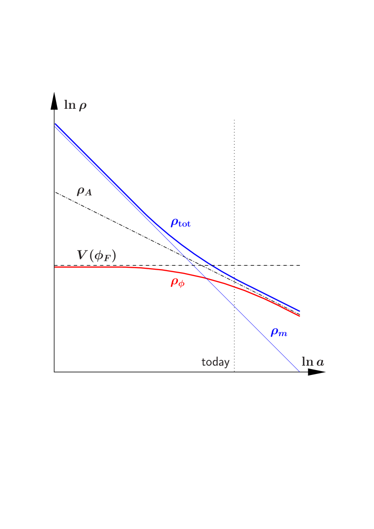
Figure 1: Schematic log-log plot of the evolution of densities in thawing quintessence with $V(\phi)\propto\phi^{-4}$. $V(\phi_{F})=\,$constant is depicted with the horizontal dashed line. The attractor (tracker) $\rho_{A}\propto a^{-2}$ is depicted with the slanted dot-dashed line. The slanted thin solid line (blue) depicts the density of matter $\rho_{m}\propto a^{-3}$, while the lower thick solid line (red) depicts $\rho_{\phi}$ and the upper thick solid line (blue) depicts the total density $\rho_{\rm tot}=\rho_{m}+\rho_{\phi}$. The present time is shown with the vertical dotted line. As evident in the figure, recently the density of quintessence unfreezes in an attempt to follow the tracker. Today $\rho_{m}<\rho_{\phi}<\rho_{A}<V(\phi_{F})$. Note however, that the tracker solution is not valid after the end of the matter era and quintessence is expected to undergo slow-roll down its potential.

However, the actual situation is more complicated. Indeed, when $V(\phi_{F})\simeq\rho_{A}$, we expect quintessence to unfreeze and start slow-rolling in an attempt to follow the tracker, as shown in Fig. 1. This however, is undermined by the fact that the tracker solution is losing its validity at present because we are no more in the pure matter era and the dark energy is about to dominate the Universe. Therefore, we should numerically investigate the problem, which may need a slightly modified value of $M$ to work.

Preliminary study is optimistic and the resulting barotropic parameter for dark energy is within the observational bounds $-1\leq w_{\phi}\leq-0.95$ [28]. The same is true of its running. In fact, the scenario presents some distinct observational signatures, because a potentially varying $w_{\phi}$ is to be probed by forthcoming observations, such as EUCLID. We find that $\phi_{F}\geq 6.80\,m_{P}$ and $0>w_{a}\geq-0.0659$, where $w_{a}\equiv-dw_{\phi}/da|_{a=a_{0}}$, (which is well within the Planck bounds $w_{a}=-0.28^{+0.31}_{-0.27}$ [28]), with $\hat{M}=6.25\,$TeV and $a_{0}\equiv a(t_{0})$ being the scale factor at the present time. The behaviour of the barotropic parameter of quintessence $w_{\phi}$ and of the Universe $w$ is shown in Fig. 2 for the limiting case $\phi_{F}=6.80\,m_{P}$ (where $w_{a}=-0.0659$). We see that the values found satisfy the Planck bounds.

Figure 2: Behaviour of the barotropic parameter of quintessence $w_{\phi}$ (lower solid curve -blue) and of the whole Universe $w$ (upper solid curve - orange) as a function of the logarithm of the scale factor $\ln a$, which is normalised to unity today $a_{0}=1$. We see that originally the Universe is in the matter era with $w=0$ and the quintessence field is frozen with constant density $V(\phi_{F})$, such that $w_{\phi}=-1$. However, when approaching the present time (depicted by the vertical solid line - black) the quintessence unfreezes and $w_{\phi}(t)>-1$, while it also begins to dominate the Universe so that $w(t)<0$. Choosing the limiting case $\phi_{F}=6.80\,m_{P}$ the present values of $w_{\phi}$ and $w$ satisfy the Planck bounds, depicted by the horizontal lines. In the future, quintessence becomes fully dominant so $w\approx w_{\phi}$, while it slow-rolls down the quintessential tail of the scalar potential, ever more slowly, approximating $w=w_{\phi}\rightarrow-1$. It is clear that both $w_{\phi}$ and $w$ are running at present, with $w_{a}\equiv-dw_{\phi}/da|_{a=a_{0}}<0$.

From Eq. (26), taking $\phi_{F}=6.80\,m_{P}$ corresponds to choosing $Q=0.002$. Then, Eq. (12) gives $H=1.16\times 10^{-5}\,m_{P}$. Using this, Eq. (13) suggests $\lambda=1.77\times 10^{-15}$. For the inflationary observables, Eq. (16) results in $n_{s}=0.967$ and Eq. (14) gives $r=0.0130$. Both comfortably satisfy the observational bounds. The value $\hat{M}=6.25\,$TeV suggests that $M=\lambda^{-1/8}\hat{M}=4.36\times 10^{5}\,$GeV. Finally, the potential density when the field is still frozen is

$$V(\phi_{F})=\frac{\hat{M}^{8}}{\phi_{F}^{4}}=(2.36\times 10^{-3}\,{\rm eV})^{4}\,.$$ (32)

Comparing the above with $\Omega_{\Lambda}\rho_{0}$ as given in Eq. (27) we have $V(\phi_{F})/\Omega_{\Lambda}\rho_{0}=(\frac{2.36}{2.25})^{4}=1.21>1$, which agrees with the expectation that the field has unfrozen and its density at present is smaller than $V(\phi_{F})$, as suggested by Fig. 1.

Before concluding, we briefly discuss the dissipative coefficient. By considering $\Upsilon\neq\Upsilon(\phi)$ we implicitly considered the case when $\Upsilon=C_{T}T$, as in Ref. [25] (see also Ref. [30]). Then we find

$$C_{T}=3QH/T\,.$$ (33)

In order to have warm inflation $T>H$. Indeed, in Ref. [25] it is found that $T/H={\cal O}(10)$. Thus, with $Q=0.002$, Eq. (33) suggests $C_{T}\sim 10^{-3}$.

6 Conclusions

In this paper we have discussed warm quintessential inflation. As a toy model we have considered the original quintessential inflation model of Ref. [14], which is shown in Eq. (1). We stress however, that the scalar potential in Eq. (1) is only experienced during the inflation and quintessence regimes when $|\phi|\sim m_{P}$, while the field is kinetically dominated when $|\phi|\ll m_{P}$, which means that it is oblivious of the potential, when crossing the origin. Because of this fact, the exact form of the potential in Eq. (1) when $|\phi|\ll m_{P}$ should not be taken too seriously. In fact, warm quintessential inflation could in principle be a possibility when considering other models of quintessential inflation in the literature (see for example Ref. [12] and references therein).

The warm quintessential inflation model presented here appears promising for a more thorough investigation, especially of the time near the end of inflation and until reheating (which determines $N_{*}$ and indirectly affects the inflationary observables $n_{s}$ and $r$) and also of the time near the present, where there is connection with the dark energy observations. It is our intention to pursue this study, but we thought that the basic idea should be put out there first. Our promising findings suggest that modelling warm quintessential inflation can be a fruitful new avenue, especially when attempting to reconcile inflation, dark energy and the swampland conjectures.

Our paper appeared first but it was soon followed by Ref. [31], which studies a very similar model. There are aspects of the system studied where each paper focuses more than the other (for example, our work is more elaborate regarding the behaviour of the quintessence field at present) and, in that sense, both works complement each other.

Acknowledgements

We would like to thank Vahid Kamali and Charlotte Owen for discussions. KD was supported (in part) by the Lancaster-Manchester-Sheffield Consortium for Fundamental Physics under STFC grant: ST/L000520/1.

References

- [1] A. A. Starobinsky, Phys. Lett. B 91 (1980) 99 [Phys. Lett. 91B (1980) 99] [Adv. Ser. Astrophys. Cosmol. 3 (1987) 130]; K. Sato, Phys. Lett. 99B (1981) 66 [Adv. Ser. Astrophys. Cosmol. 3 (1987) 134]; D. Kazanas, Astrophys. J. 241 (1980) L59; A. H. Guth, Phys. Rev. D 23 (1981) 347 [Adv. Ser. Astrophys. Cosmol. 3 (1987) 139].
- [2] S. Perlmutter et al. [Supernova Cosmology Project Collaboration], Astrophys. J. 517 (1999) 565; A. G. Riess et al. [Supernova Search Team], Astron. J. 116 (1998) 1009.
- [3] P. J. E. Peebles and B. Ratra, Rev. Mod. Phys. 75 (2003) 559; T. Padmanabhan, Phys. Rept. 380 (2003) 235; E. J. Copeland, M. Sami and S. Tsujikawa, Int. J. Mod. Phys. D 15 (2006) 1753.
- [4] G. Obied, H. Ooguri, L. Spodyneiko and C. Vafa, arXiv:1806.08362 [hep-th]; H. Ooguri, E. Palti, G. Shiu and C. Vafa, Phys. Lett. B 788 (2019) 180.
- [5] P. Agrawal, G. Obied, P. J. Steinhardt and C. Vafa, Phys. Lett. B 784 (2018) 271;
- [6] Y. Akrami, R. Kallosh, A. Linde and V. Vardanyan, Fortsch. Phys. 67 (2019) no.1-2, 1800075.
- [7] S. K. Garg and C. Krishnan, arXiv:1807.05193 [hep-th]; W. H. Kinney, S. Vagnozzi and L. Visinelli, Class. Quant. Grav. 36 (2019) no.11, 117001; A. Achúcarro and G. A. Palma, JCAP 1902 (2019) 041; A. Kehagias and A. Riotto, Fortsch. Phys. 66 (2018) no.10, 1800052.
- [8] S. Das, Phys. Rev. D 99 (2019) no.8, 083510; S. Das, Phys. Rev. D 99 (2019) no.6, 063514; M. Motaharfar, V. Kamali and R. O. Ramos, Phys. Rev. D 99 (2019) no.6, 063513.
- [9] A. Berera, Phys. Rev. Lett. 75 (1995) 3218.
- [10] C. Wetterich, Nucl. Phys. B 302 (1988) 668; B. Ratra and P. J. E. Peebles, Phys. Rev. D 37 (1988) 3406; P. G. Ferreira and M. Joyce, Phys. Rev. D 58 (1998) 023503; R. R. Caldwell, R. Dave and P. J. Steinhardt, Phys. Rev. Lett. 80 (1998) 1582.
- [11] M. Cicoli, S. De Alwis, A. Maharana, F. Muia and F. Quevedo, Fortsch. Phys. 67 (2019) no.1-2, 1800079; L. Heisenberg, M. Bartelmann, R. Brandenberger and A. Refregier, Phys. Rev. D 98 (2018) no.12, 123502; Sci. China Phys. Mech. Astron. 62 (2019) no.9, 990421.
- [12] K. Dimopoulos and C. Owen, JCAP 1706 (2017) no.06, 027; K. Dimopoulos, L. Donaldson Wood and C. Owen, Phys. Rev. D 97 (2018) no.6, 063525.
- [13] M. W. Hossain, R. Myrzakulov, M. Sami and E. N. Saridakis, Phys. Rev. D 90 (2014) no.2, 023512; Phys. Rev. D 89 (2014) no.12, 123513; Int. J. Mod. Phys. D 24 (2015) no.05, 1530014; C. Q. Geng, M. W. Hossain, R. Myrzakulov, M. Sami and E. N. Saridakis, Phys. Rev. D 92 (2015) no.2, 023522.
- [14] P. J. E. Peebles and A. Vilenkin, Phys. Rev. D 59 (1999) 063505.
- [15] M. Giovannini, arXiv:1905.06182 [gr-qc]; . Haro, W. Yang and S. Pan, JCAP 1901 (2019) no.01, 023.
- [16] R. J. Scherrer and A. A. Sen, Phys. Rev. D 77 (2008) 083515; T. Chiba, Phys. Rev. D 79 (2009) 083517 Erratum: [Phys. Rev. D 80 (2009) 109902].
- [17] B. Spokoiny, Phys. Lett. B 315 (1993) 40; M. Joyce and T. Prokopec, Phys. Rev. D 57 (1998) 6022.
- [18] L. H. Ford, Phys. Rev. D 35 (1987) 2955; E. J. Chun, S. Scopel and I. Zaballa, JCAP 0907 (2009) 022.
- [19] G. N. Felder, L. Kofman and A. D. Linde, Phys. Rev. D 59 (1999) 123523; A. H. Campos, H. C. Reis and R. Rosenfeld, Phys. Lett. B 575 (2003) 151.
- [20] B. Feng and M. z. Li, Phys. Lett. B 564 (2003) 169; J. C. Bueno Sanchez and K. Dimopoulos, JCAP 0711 (2007) 007.
- [21] K. Dimopoulos and T. Markkanen, JCAP 1806 (2018) no.06, 021.
- [22] T. Opferkuch, P. Schwaller and B. A. Stefanek, arXiv:1905.06823 [gr-qc].
- [23] S. Ahmad, R. Myrzakulov and M. Sami, Phys. Rev. D 96 (2017) no.6, 063515.
- [24] L. M. H. Hall, I. G. Moss and A. Berera, Phys. Rev. D 69 (2004) 083525; I. G. Moss and C. M. Graham, Phys. Rev. D 78 (2008) 123526; M. Bastero-Gil, A. Berera and R. O. Ramos, JCAP 1107 (2011) 030; R. O. Ramos and L. A. da Silva, JCAP 1303 (2013) 032.
- [25] M. Bastero-Gil, S. Bhattacharya, K. Dutta and M. R. Gangopadhyay, JCAP 1802 (2018) no.02, 054.
- [26] R. Arya, A. Dasgupta, G. Goswami, J. Prasad and R. Rangarajan, JCAP 1802 (2018) no.02, 043; M. Benetti and R. O. Ramos, Phys. Rev. D 95 (2017) no.2, 023517; S. Bartrum, M. Bastero-Gil, A. Berera, R. Cerezo, R. O. Ramos and J. G. Rosa, Phys. Lett. B 732 (2014) 116; M. Bastero-Gil, A. Berera and R. O. Ramos, JCAP 1107 (2011) 030; M. Bastero-Gil and A. Berera, Phys. Rev. D 76 (2007) 043515.
- [27] M. Bastero-Gil and A. Berera, Phys. Rev. D 71 (2005) 063515; N. Videla and G. Panotopoulos, Phys. Rev. D 97 (2018) no.12, 123503.
- [28] Y. Akrami et al. [Planck Collaboration], arXiv:1807.06211 [astro-ph.CO]; N. Aghanim et al. [Planck Collaboration], arXiv:1807.06209 [astro-ph.CO].
- [29] P. J. Steinhardt, L. M. Wang and I. Zlatev, Phys. Rev. D 59 (1999) 123504; T. Chiba, A. De Felice and S. Tsujikawa, Phys. Rev. D 87 (2013) no.8, 083505; I. Zlatev, L. M. Wang and P. J. Steinhardt, Phys. Rev. Lett. 82 (1999) 896.
- [30] M. Bastero-Gil, A. Berera, R. O. Ramos and J. G. Rosa, Phys. Rev. Lett. 117 (2016) no.15, 151301; M. Bastero-Gil, A. Berera, R. Hernández-Jiménez and J. G. Rosa, Phys. Rev. D 98 (2018) no.8, 083502.
- [31] J. G. Rosa and L. B. Ventura arXiv:1906.11835 [hep-ph].