Spectral Noncommutative Geometry, Standard Model and all that

We review the approach to the standard model of particle interactions based on spectral noncommutative geometry. The paper is (nearly) self-contained and presents both the mathematical and phenomenological aspects. In particular the bosonic spectral action and the fermionic action are discussed in detail, and how they lead to phenomenology. We also discuss the Euclidean vs. Lorentz issues and how to go beyond the standard model in this framework.

Keywords: Noncommutative Geometry, Standard Model;
Pacs 02.40 Gh, 11.10 Nx, 12-60.-i.

1 Introduction

The aim of this review is to present the standard model of particle interaction as a particular geometry of spacetime, a noncommutative geometry. The standard model is a very successful theory, and it seems to be working well beyond “factory specifications”. The CERN measurement of the mass of the Higgs mass has been the crowing of several decades of confirmations of the model. Of course not everything is understood, and there are loose ends which may lead to significative advances. Yet little is know about the origin of it. Why among all possible Yang-Mills gauge theories nature has privileged a particular set of particles transforming under a particular representation? A full answer to these questions will of course not be given here, nevertheless we are convinced that a geometrical vision of the standard model may be a key to progress. There are other reasons to consider spacetime as a noncommutative geometry, mainly coming from quantum gravity, where the object to quantize is spacetime itself.

The noncommutative geometry of the standard model presents a very mild version of noncommutativity. Spacetime itself is still an ordinary (possibly curved) manifold, but it is tensor multiplied times a noncommutative, but finite geometry: a matrix algebra. This geometric constructions correspond to the so called spectral triples, which we discuss in the present review. Noncommutative geometry is then used to give a spectral view of the geometry, its symmetries, and the action. There are several important features of this view. The first is that the Higgs particle is on the same footing of the other bosons, it represents the fluctuations of the internal geometry. It becomes another “intermediate boson”, except that its “intermediate boson” nature refers to the internal space, and is therefore a scalar from the continuous spacetime point of view. The other important point is that not any Yang-Mills gauge theory can be described in this framework, on the contrary, if one makes the request that the internal finite dimensional space is the noncommutative equivalent of a manifold, then very few models survive, the standard model among them, or Pati-Salam, but none of the other Grand Unified Theories such as SU(5) or SO(10).

The starting point of noncommutative geometry is based on the spectra of operators, and the action is also based on the spectral data of a generalised Dirac operator. Using the mass (or rather the Yukawa couplings) of known fermions as input in this generalised operator, it is possible to write the action of the standard model, in a curved gravitational background (which is not quantised). The action is composed of a scalar product and a trace properly regularised, and is given at a particular point in the renormalisation flow. In this point the three fundamental interaction have the same strength. It is known that such a point (in the absence of new physics) exists only approximatively, but this gives the possibility to calculate quantities such as the mass of the Higgs. In its bare formulation this number is not the correct one, but further refinements of the model make it compatible with experiment.

We will start our review with a brief recap of the standard model coupled with gravity. This will help not only to set notations, but also to understand what we want to explain. The following section introduces noncommutative geometry from a spectral point of view, as pioneered by Connes. The two previous aspects come together in the fourth section, where the standard model as an almost commutative geometry is presented from a geometrical point of view. The connection with physics is further developed in the following two sections, dedicated to the description of the spectral action and the “numbers” that one can produce from these models. Sections 7 and 8 describe further developments which go beyond the standard model, while Section 9 discusses the issue of the Lorentzian vs. Euclidean signature of the model. A final section concludes the review and gives some pointers for further developments.

References to original work are given when the topic is introduced, but here we would like to refer to other, often complementary, reviews. One of us (FL) gave series of lectures on these topics at the Cimpa School Noncommutative Geometry and Applications to Quantum Physics in Qui Nhon (Vietnam) in 2017, at the COST action training school in Corfu (2017) and at the Bose Research center in Kolkata (2018). A reduced and partial version of these lectures can be fount in [95]. A complete reference, from a mathematician point of view is in a book by W. Van Suijlekom [135], see also his more recent review with Chamseddine [41].

We conclude this introduction with a little bit of history, without any pretence to be complete. The first works on the Higgs as a fluctuation of a noncommutative geometry are in the work of Dubois-Violette, Kerner and Madore [64] and Connes and Lott [47]. For an early discussion of the Higgs (before the spectral action) see also [120]. A lot of preparatory work was done by the Marseille group, notably Daniel Kastler, Bruno Iochum and Thomas Schucker and several young people, in a series of papers lasting over a decade. No review would be complete without mentioning their work. One of the latest review by T. Schucker, which still has some fresh interest, is [118]. A more recent “friendly” overview is [122].

2 The Standard Model and Gravity

Our understanding of fundamental interactions is based on the two pillars: the Standard Model of particle physics and the General Relativity. The Standard Model (SM) is a quantum field theory which addresses the electromagnetic, weak and strong interactions of elementary particles. It had an impressive successes, predicting, for example, the W, Z and Higgs bosons well before experiments demonstrated their existence. General Relativity (GR) describes gravity in terms of differential geometry. It also is supported by a several experiments, starting from the perihelion precession of Mercury, up to modern astrophysical observations of binary pulsars dynamics.

Below we briefly review the action for these two theories. The aim of this microreview is twofold. On the one hand we set the notations, on the other we outline some relevant aspects of SM which are closely related to the spectral action principle. We use the “recent version” of the Standard Model incorporating right handed neutrino. Then discuss some aspects of the renormalization group flow. One of the aims of this review is to show how the SM action can be obtained from the spectral Noncommutative Geometry (NCG), which treats gauge and gravitational degrees of freedom on an equal footing. Therefore we introduce the SM action directly on a curved gravitational background and after that discuss the gravitational action as a part of the bosonic action.

2.1 The Classical Fermionic action of Standard Model

The fermions of the Standard Model are combined in multiplets according to their transformation properties upon the action of the gauge group $SU(3)\times SU(2)\times U(1)$. Note one important aspect: all the multiplets transform according to either fundamental or trivial representations of $SU(3)$ and $SU(2)$. The action of the abelian subgroup $U(1)$ is defined by the hypercharge $Y$. These transformation properties are summarised in Tab. 1.

	$\boldsymbol{\mathrm{v}}_{\mathcal{R}}$	$\boldsymbol{\mathrm{e}}_{\mathcal{R}}$	$\boldsymbol{\mathrm{L}}_{\mathcal{L}}$	$\boldsymbol{\mathrm{u}}_{\mathcal{R}}$	$\boldsymbol{\mathrm{d}}_{\mathcal{R}}$	$\boldsymbol{\mathrm{Q}}_{\mathcal{L}}$
SU(3)	t	t	t	f	f	f
SU(2)	t	t	f	t	t	f
U(1)	0	-2	-1	4/3	-2/3	1/3

Table 1: Representations of the gauge subgroups on various fermionic multiplets of the Standard Model. For the nonabelian subgroups $SU(3)$ and $SU(2)$ the letters “f” and “t” indicate a fundamental and a trivial representations respectively. For the abelian subgroup $U(1)$ we specify the hypercharge $Y$.

Hereafter $\boldsymbol{\mathrm{v}}$, $\boldsymbol{\mathrm{e}}$, $\boldsymbol{\mathrm{u}}$ and $\boldsymbol{\mathrm{d}}$ indicate neutrinos, electron-like leptons, upper and down like quarks respectively. Moreover $\boldsymbol{\mathrm{Q}}_{\mathcal{L}}$ corresponds to the quark doublets $(\boldsymbol{\mathrm{u}}_{\mathcal{L}},\boldsymbol{\mathrm{d}}_{\mathcal{L}})$ while $\boldsymbol{\mathrm{L}}_{\mathcal{L}}$ corresponds to the lepton doublets $(\boldsymbol{\mathrm{v}}_{\mathcal{L}},\boldsymbol{\mathrm{e}}_{\mathcal{L}})$. By boldface characters we indicate that the multiplets have to be replicated by three generations, for example $\boldsymbol{\mathrm{e}}=(e,\mu,\tau)$ and so on. The subscripts $\mathcal{L}$ and $\mathcal{R}$ indicate the chirality of the fermions $\psi$ from the corresponding multiplets. By definition the left and the right handed fermions satisfy:

$$\psi_{\mathcal{L}}=\frac{1}{2}\left(1-\gamma^{5}\right)\psi_{\mathcal{L}},\quad\quad\psi_{\mathcal{R}}=\frac{1}{2}\left(1+\gamma^{5}\right)\psi_{\mathcal{R}}.$$ (2.1)

The fermionic action of the Standard Model reads:

$$S^{\rm{M}}_{F} = \int d^{4}x\sqrt{-g^{\rm M}}\left\{\right.i\overline{\left(\boldsymbol{\mathrm{u}}_{\mathcal{R}}\right)}\not{\nabla}_{\mathrm{M}}\boldsymbol{\mathrm{u}}_{\mathcal{R}}+i\overline{\left(\boldsymbol{\mathrm{d}}_{\mathcal{R}}\right)}\not{\nabla}_{\mathrm{M}}\boldsymbol{\mathrm{d}}_{\mathcal{R}}+i\overline{\left(\boldsymbol{\mathrm{Q}}_{\mathcal{L}}\right)}\not{\nabla}_{\mathrm{M}}\boldsymbol{\mathrm{Q}}_{\mathcal{L}}$$ (2.2)

$$+ i\overline{\left(\boldsymbol{\mathrm{v}}_{\mathcal{R}}\right)}\not{\nabla}_{\mathrm{M}}\boldsymbol{\mathrm{v}}_{\mathcal{R}}+i\overline{\left(\boldsymbol{\mathrm{e}}_{\mathcal{R}}\right)}\not{\nabla}_{\mathrm{M}}\boldsymbol{\mathrm{e}}_{\mathcal{R}}+i\overline{\left(\boldsymbol{\mathrm{L}}_{\mathcal{L}}\right)}\not{\nabla}_{\mathrm{M}}\boldsymbol{\mathrm{L}}_{\mathcal{L}}$$

$$- \left[\overline{\left(\boldsymbol{\mathrm{Q}}_{\mathcal{L}}\right)}\left[\hat{y}^{\dagger}_{u}\otimes\tilde{H}\right]\boldsymbol{\mathrm{u}}_{\mathcal{R}}+\overline{\left(\boldsymbol{\mathrm{Q}}_{\mathcal{L}}\right)}\left[\hat{y}_{d}^{\dagger}\otimes H\right]\boldsymbol{\mathrm{d}}_{\mathcal{R}}+\right.$$

$$+ \overline{\left(\boldsymbol{\mathrm{L}}_{\mathcal{L}}\right)}\left[\hat{Y}^{\dagger}_{u}\otimes\tilde{H}\right]\boldsymbol{\mathrm{v}}_{\mathcal{R}}+\overline{\left(\boldsymbol{\mathrm{L}}_{\mathcal{L}}\right)}\left[\hat{Y}^{\dagger}_{d}\otimes\ H\right]\boldsymbol{\mathrm{e}}_{\mathcal{R}}$$

$$+ \frac{1}{2}\overline{\left(C_{\rm M}\boldsymbol{\mathrm{v}}_{\mathcal{R}}\right)}\left[\hat{y}_{M}^{\dagger}\right]\mathrm{M}_{R}\boldsymbol{\mathrm{v}}_{\mathcal{R}}\left.\left.+\mbox{c.c.}\right]\right\}.$$

Below we clarify the meaning of various quantities which enter in this formula, considering inputs of various nature separately. Note that this structure, in addition to the fermions, contains all other dynamical degrees of freedom: the vector gauge bosons, the scalar bosons and gravity which appears via the vierbeins. In some sense this observation gives a heuristic basis for the spectral action principle, which we discuss in Sec. 4.

Geometric input and spin structures.

The label “${\rm{M}}$” in (2.2) indicates the fact that we are dealing with the Minkowskian theory, i.e. the metric tensor $g^{\mathrm{M}}_{\mu\nu}$ has signature $(+,-,-,-)$. As we will see in Sec.3, in the NCG spectral approach an important role is played by the Euclidean structures, which we will label by “$\mathrm{E}$”. The quantity $g^{\rm M}$ is the determinant of the metric tensor. The expression $\not{\nabla}_{\mathrm{M}}$ is a contraction over the world index of the $\gamma^{\mu}_{\mathrm{M}}$ and the covariant derivatives $\nabla_{\mu}^{\mathrm{M}}$. These can be obtained from the flat gamma matrices $\gamma^{a}_{\mathrm{M}}$, which satisfy

$$\left\{\gamma^{a}_{\mathrm{M}},\gamma^{b}_{\mathrm{M}}\right\}=\eta^{ab}\mathbb{1}_{4},$$ (2.3)

contracting them with the vierbeins $e_{a}^{\mu}$ over the flat (tangential) index $a$:

$$\gamma^{\mu}_{\mathrm{M}}=e^{\mu}_{a}\gamma^{a}_{\mathrm{M}}.$$ (2.4)

The quantities

$$\eta^{ab}=\mathrm{diag}(+1,-1,-1,-1)=\eta_{ab}$$ (2.5)

and $\mathbb{1}_{4}$, which enter in (2.3), stand for the flat Minkowskian metric and for the unit four by four matrix in spinorial indexes respectively. The vierbeins satisfy

$$e^{\mu}_{a}e^{\nu}_{b}\,g^{\mathrm{M}}_{\mu\nu}=\eta_{ab}.$$ (2.6)

The symbol bar in (2.2) indicates the Dirac conjugation of spinors according to the following rule

$$\bar{\psi}=\psi^{\dagger}\gamma^{0}_{\mathrm{M}},$$ (2.7)

where $\dagger$ stands for the Hermitian conjugation and $\gamma^{0}_{\mathrm{M}}$ is the 0-th flat Dirac matrix. The covariant derivative $\nabla_{\mu}^{\mathrm{M}}$ has the structure

$$\nabla_{\mu}^{\mathrm{M}}=\partial_{\mu}-{\mathrm{i}}\mathcal{A}_{\mu}-\frac{{\mathrm{i}}}{2}\omega_{\mu}^{\mathrm{M}},$$ (2.8)

where $\mathcal{A}_{\mu}$ stands for the gauge connection, which acts on various fermionic multiplets in a different way, and which we discuss in details below. The spin-connection

$$\omega_{\mu}^{\mathrm{M}}=\left[\omega_{\mu}^{ab}\right]^{\mathrm{M}}\sigma^{\mathrm{M}}_{ab},$$ (2.9)

is common for all fermionic multiplets. In this formula

$$\left[\omega_{\mu}^{ab}\right]^{\mathrm{M}}=e^{a}_{\nu}\,g_{\mathrm{M}}^{\nu\xi}\,\partial_{\mu}e^{b}_{\xi}+e^{a}_{\nu}\left[\Gamma^{\nu}_{\mu\xi}\right]^{\mathrm{M}}e^{b}_{\rho}\,g_{\mathrm{M}}^{\rho\xi},$$ (2.10)

and

$$\sigma^{\mathrm{M}}_{ab}=\frac{{\mathrm{i}}\left[\gamma^{c}_{\mathrm{M}},\gamma^{d}_{\mathrm{M}}\right]}{4}\,\eta_{ac}\eta_{bd},$$ (2.11)

stand for generators of the defining representation of $Spin(1,3)$. These four by four matrices act on the spinorial index of various multiplets. In  (2.10) the quantities $\left[\Gamma^{\nu}_{\mu\xi}\right]^{\mathrm{M}}$ are the Christoffel symbols of the second kind, which are computed with the Minkowskian metric $g_{\mu\nu}^{\mathrm{M}}$. For a generic metric tensor $g_{\mu\nu}$ these read

$$\Gamma_{\nu\rho}^{\mu}\left[g_{\mu\nu}\right]\equiv\frac{1}{2}\,g^{\mu\lambda}\left(\partial_{\rho}g_{\lambda\nu}+\partial_{\nu}g_{\lambda\rho}-\partial_{\lambda}g_{\nu\rho}\right).$$ (2.12)

In (2.10) and (2.12) we used the metric tensor with two upper indexes and the vierbeins with lower world and upper flat indexes. For any given metric tensor $g_{\mu\nu}$ and a vierbein field $e_{a}^{\mu}$ seen as square matrices in their indexes these objects are nothing but the corresponding inverse matrices:

$$g_{\mu\nu}g^{\nu\lambda}=\delta_{\mu}^{\lambda},\quad e_{\mu}^{a}e^{\mu}_{b}=\delta^{a}_{b},\quad e_{\mu}^{a}e^{\nu}_{a}=\delta_{\mu}^{\nu}.$$ (2.13)

The spin connection renders the local “pseudo-rotational” invariance of  (2.2) upon simultaneous local $SO(1,3)$ pseudo-rotations of vierbeins and the corresponding $Spin(1,3)$ transformations of fermionic fields. In conclusion we notice that the fermionic action, being a scalar, remains invariant upon local diffeomorhisms. We remind that upon these transformations fermionic fields transform as scalars.

Gauge input.

Let us take a closer look at the gauge connection $\mathcal{A}$, which enters in the covariant derivative (2.8). For various fermionic multiplets the gauge connection reads:

$$\mathcal{A}^{\boldsymbol{\mathrm{v}}_{\mathcal{R}}}_{\mu} = g_{1}\,Y_{\boldsymbol{\mathrm{v}}_{\mathcal{R}}}\,B_{\mu},$$

$$\mathcal{A}^{\boldsymbol{\mathrm{e}}_{\mathcal{R}}}_{\mu} = g_{1}\,Y_{\boldsymbol{\mathrm{e}}_{\mathcal{R}}}\,B_{\mu},$$

$$\mathcal{A}^{\boldsymbol{\mathrm{L}}_{\mathcal{L}}}_{\mu} = g_{1}\,Y_{\boldsymbol{\mathrm{L}}_{\mathcal{L}}}\,B_{\mu}+g_{2}\,W_{\mu},$$

$$\mathcal{A}^{\boldsymbol{\mathrm{u}}_{\mathcal{R}}}_{\mu} = g_{1}\,Y_{\boldsymbol{\mathrm{u}}_{\mathcal{R}}}\,B_{\mu}+g_{3}\,G_{\mu},$$

$$\mathcal{A}^{\boldsymbol{\mathrm{d}}_{\mathcal{R}}}_{\mu} = g_{1}\,Y_{\boldsymbol{\mathrm{d}}_{\mathcal{R}}}\,B_{\mu}+g_{3}\,G_{\mu},$$

$$\mathcal{A}^{\boldsymbol{\mathrm{Q}}_{\mathcal{L}}}_{\mu} = g_{1}\,Y_{\boldsymbol{\mathrm{Q}}_{\mathcal{L}}}\,B_{\mu}+g_{2}\,W_{\mu}+g_{3}\,G_{\mu},$$ (2.14)

where the superscripts indicate the corresponding multiplets. The quantities $g_{1}$, $g_{2}$ and $g_{3}$ stand for the $U(1)$, $SU(2)$ and $SU(3)$ gauge coupling constants respectively, $B_{\mu}$ is a real vector field, and the abelian hypercharges $Y$ for various multiplets are collected in Tab. 1. The matrix valued fields $W_{\mu}$ and $G_{\mu}$ are built from the real vector fields $W_{\mu}^{\alpha}$, $\alpha=1,2,3$ and $G_{\mu}^{j}$, $j=1,\ldots,8$ according to the formulas

$$W_{\mu} = \frac{\sigma_{\alpha}}{2}\cdot W_{\mu}^{\alpha},$$

$$G_{\mu} = \frac{\lambda_{j}}{2}\cdot G_{\mu}^{j},$$ (2.15)

act on the Weak isospin index of left doublets and on the colour index of quark triplets. The 2 by 2 matrices $\sigma_{\alpha}$ are Pauli matrices, and $\lambda_{i}$ stand for the 3 by 3 Gell-Mann matrices.

A presence of the gauge fields in the covariant derivatives guarantees a local $SU(3)\times SU(2)\times U(1)$ gauge invariance of the kinetic terms for fermions, which are given by the first two lines of (2.2).

Scalars the Dirac mass terms.

The third and the fourth lines of  (2.2) define the Dirac mass terms. The quantities $\hat{Y}_{u}$, $\hat{Y}_{d}$, $\hat{y}_{u}$, $\hat{y}_{d}$ are arbitrary (dimensionless) complex 3 by 3 Yukawa matrices which act on the generation indices of fermionic multiplets.

According to our conventions the quantity

$$H=\left(\begin{array}[]{c}H^{\mathrm{up}}\\ H^{\mathrm{down}}\end{array}\right)$$ (2.16)

is a weak isospin doublet of scalar fields, which transforms according to the fundamental representation of the $SU(2)$ gauge subgroup and has the hypercharge $Y_{H}=1$. By definition the “charged conjugated” scalar doublet equals to

$$\tilde{H}={\mathrm{i}}\sigma_{2}H^{*},$$ (2.17)

where * stands for the complex conjugation and $\sigma_{2}$ is the second Pauli matrix. One can easily see that $\tilde{H}$ transforms as $H$ under $SU(2)$ transformations, however it has opposite hypercharge: $Y_{\tilde{H}}=-1$. These transformation properties ensure gauge invariance of the Dirac mass terms. We emphasise that $H$ and $\tilde{H}$ are contracted with fermionic multiplets over the $SU(2)$-representation indexes. To emphasize the fact that the Yukawa matrices act on different indices we have written in (2.2) explicitly the tensor product $\otimes$, which is usually omitted.

Charge conjugation and the Majorana mass terms.

The Majorana mass terms, which are given by the last line of (2.2). The quantity $\hat{y}_{M}$ is a 3 by 3 complex matrix acting on a generation index, $\mathrm{M}_{R}$ is the dimensionful constant, which sets the Majorana mass scale for the right handed neutrinos, and the operation

$$C_{\mathrm{M}}=-{\mathrm{i}}\gamma^{2}_{\mathrm{M}}\,\circ\,\mbox{complex conjugation},$$ (2.18)

is the Minkowskian charge conjugation.

The charged conjugated spinor multiplet and the original one transform in the same way upon the the $Spin(1,3)$ transformations, but upon local gauge transformations and global $U(1)$ transformations (e.g. the lepton and baryon number accidental symmetries) the charged conjugated multiplet transforms according to the complex conjugated representation. In particular the Majorana mass terms explicitly violate the lepton number conservation.

2.2 Bosonic action

The bosonic action of SM bosons together with gravity is given by

$$S_{B}^{\mathrm{M}}=\int d^{4}x\,\sqrt{-g^{\mathrm{M}}}\left(L_{\rm g}+L_{\rm s}+L_{\rm gr}\right),$$ (2.19)

where $L_{\rm g}$, $L_{\rm s}$ and $L_{\rm gr}$ stand for the gauge, scalar and the gravitational Lagrangians respectively. The gauge Lagrangian is a sum of the Yang-Mills Lagrangians for the nonabelian vector fields $G_{\mu}$ and $W_{\mu}$ and the Maxwell Lagrangian for the abelian vector field $B_{\mu}$:

$$L_{\rm g}=-\frac{1}{4}G_{\mu\nu}^{j}G^{\mu\nu\,j}-\frac{1}{4}W_{\mu\nu}^{\alpha}W^{\mu\nu\,\alpha}-\frac{1}{4}B_{\mu\nu}B^{\mu\nu}.$$ (2.20)

here the quantities $G_{\mu\nu}^{j}$, $W^{\mu\nu\,\alpha}$ and $B_{\mu\nu}$ stand for the field-strength tensors associated with the corresponding gauge connections:

$$G_{\mu\nu}^{i} = \partial_{\mu}G^{i}_{\nu}-\partial_{\nu}G^{i}_{\mu}+g_{3}f^{ijk}G_{\mu}^{j}G_{\nu}^{k},$$

$$W_{\mu\nu}^{\alpha} = \partial_{\mu}W^{\alpha}_{\nu}-\partial_{\nu}W^{\alpha}_{\mu}+g_{2}f^{\alpha\beta\gamma}W_{\mu}^{\beta}W_{\nu}^{\gamma},$$

$$B_{\mu\nu} = \partial_{\mu}B_{\nu}-\partial_{\nu}B_{\mu}.$$ (2.21)

The Lagrangian for the Higgs scalar $H$, which is minimally coupled to gravity, reads:

$$L_{\rm s}=g^{\mu\nu}_{\mathrm{M}}\nabla_{\mu}H^{\dagger}\nabla_{\nu}H-V(H).$$ (2.22)

According to the transformation properties of the Higgs doublet upon the action of the gauge group, which we discussed above, the covariant derivative, which appears in the kinetic terms, involves the $SU(2)$ and the $U(1)$ gauge connections:

$$\nabla_{\mu}H=\left(\partial_{\mu}-{\mathrm{i}}g_{1}\,Y_{H}\,B_{\mu}-{\mathrm{i}}g_{2}W_{\mu}\right)H.$$ (2.23)

The potential term $V(H)$ is the famous Mexican hat potential, which plays a crucial role in the Higgs mechanism of a spontaneous symmetry breaking:

$$V(H)=-\mathfrak{m}^{2}H^{\dagger}H+\lambda\left(H^{\dagger}H\right)^{2}.$$ (2.24)

In this formula $\lambda$ is a positive dimensionless quartic coupling constant. The quantity $\mathfrak{m}$ is a real constant of the dimension of a mass - the so called “mass parameter” (not to be confused with the actual mass!). This potential has a family of nontrivial minima $\left(H^{\dagger}H\right)_{0}^{2}$, which are usually parametrised by the constant

$$v=\sqrt{\left(H^{\dagger}H\right)_{0}^{2}},$$ (2.25)

which is called the “Higgs vacuum expectation value”. Its experimental value is 246 GeV.

Let us fix the notations for the Riemann tensor, Ricci tensor and the scalar curvature for generic metric tensor $g_{\mu\nu}$

$$R^{\mu}_{\leavevmode\nobreak\ \nu\rho\sigma}\left[g_{\mu\nu}\right] = \partial_{\sigma}\Gamma^{\mu}_{\nu\rho}-\partial_{\rho}\Gamma^{\mu}_{\nu\sigma}+\Gamma^{\lambda}_{\nu\rho}\Gamma^{\mu}_{\lambda\sigma}-\Gamma^{\lambda}_{\nu\sigma}\Gamma^{\mu}_{\lambda\rho}.$$

$$R_{\mu\nu}\left[g_{\mu\nu}\right]=R^{\sigma}_{\leavevmode\nobreak\ \mu\sigma\nu} = \partial_{\nu}\Gamma^{\sigma}_{\mu\sigma}-\partial_{\sigma}\Gamma^{\sigma}_{\mu\nu}+\Gamma^{\lambda}_{\mu\sigma}\Gamma^{\sigma}_{\lambda\nu}-\Gamma^{\lambda}_{\mu\nu}\Gamma^{\sigma}_{\lambda\sigma}.$$

$$R\left[g_{\mu\nu}\right] = g^{\mu\nu}\left\{\partial_{\nu}\Gamma^{\sigma}_{\mu\sigma}-\partial_{\sigma}\Gamma^{\sigma}_{\mu\nu}+\Gamma^{\lambda}_{\mu\sigma}\Gamma^{\sigma}_{\lambda\nu}-\Gamma^{\lambda}_{\mu\nu}\Gamma^{\sigma}_{\lambda\sigma}\right\}.$$ (2.26)

Now we introduce the the gravitational Einstein-Hilbert action:

$$L_{\rm gr}=-\lambda_{\mathrm{c}}\,+\,\frac{M_{\rm Pl}^{2}}{16\pi}R\left[g_{\mu\nu}^{\rm M}\right].$$ (2.27)

The quantity $\lambda_{\mathrm{c}}$ is a real parameter of the dimension $[\mathrm{mass}^{4}]$, which defines a cosmological term. The quantity $M_{\rm Pl}$ is a parameter of the dimension of a mass, whose experimentally observed value is of the order of $10^{19}$ GeV.

2.3 Renormalization group flow: relevant aspects

Upon quantisation various couplings of the Standard Model exhibit a dependence on the energy scale - the normalisation point $\mu$. Such a dependence is often called the renormalisation group (RG) flow or the RG running, and it is described mathematically by the RG equations: an autonomous system of the first order ordinary differential equations. In the spectral approach to the SM an important role is played by the RG flow of the gauge couplings. As we will see in Sect. 6, it provides us with a range of values for the UV cutoff $\Lambda$, which is needed to define the bosonic spectral action, therefore let us focus on it. The RG equations for the gauge coupling constants $g_{i}$ read:

$$\mu\frac{{\mathrm{d}}g_{i}}{{\mathrm{d}}\mu}=\beta_{g_{i}}$$ (2.28)

where the righthand sides are called the beta-functions of the corresponding couplings. These beta functions, generally speaking, depend on all the coupling constants, which are involved in the model and can be computed in a perturbative way via the loop expansion [98, 99, 100].

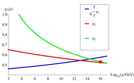
Figure 2.1: The RG running of the gauge couplings $g_{i}$, $i=1,2,3$ in the Standard Model.

At the one loop approximation the beta functions for the gauge couplings are given by

$$\beta_{g_{1}} = \frac{g_{1}^{3}}{16\pi^{2}}\frac{41}{6},$$

$$\beta_{g_{2}} = -\frac{g_{2}^{3}}{16\pi^{2}}\frac{19}{6},$$

$$\beta_{g_{3}} = -\frac{g_{3}^{3}}{16\pi^{2}}7,$$ (2.29)

therefore at this approximation the system (2.28) is closed, and moreover the three equations are not coupled with each other. The initial conditions for these equations are can be taken from the experiment, in particular at $\mu=M_{Z}$:

$$g_{1}(M_{Z})=0.3575\,,\,\,g_{2}(M_{Z})=0.6514\,,\,\,g_{3}(M_{Z})=1.1221.$$ (2.30)

and the corresponding solutions are plotted on Fig. 2.1.

Using the results of [98, 99, 100] one can check that the two loop corrections that do not change this plot significantly. Even though the gauge couplings do not exhibit an exact unification at a single scale $\mu$, there is a some sort of an approximate unification when $\mu$ varies from $10^{14}$GeV to $10^{17}$GeV. This observation, as we will see, is very important for the spectral action principle.

3 Geometry from Algebras

In this chapter we present an enlarged definition of geometry, which could encompass also spaces such as the quantum phase space of particles, or the standard model. Taking inspiration from position and momentum in quantum mechanics, we aim at describing geometries (both ordinary or noncommutative) using the spectral properties of a (possibly noncommuting) algebra of operators. We will introduce the necessary mathematical objects keeping the mathematical rigour at a minimum, and with examples mostly relating to ordinary geometry. More details for the construction, still for a nonmathematical audience are in [95]. The reader interested to details may wish to look at one of the several monographs on the subject, for example [44, 93, 78, 48, 10].

3.1 Algebras

An associative algebra $\mathcal{A}$ over the field of complex numbers $\mathbb{C}$ is a vector space on $\mathbb{C}$, so that every object like $\alpha a+\beta b$ with $\alpha,\beta\in\mathcal{\mathbb{C}}$ and $a,b\in\mathcal{A}$, belongs to $\mathcal{A}$, equipped with a product $\mathcal{A}\times\mathcal{A\rightarrow A}$ which is associative, i.e. $(ab)c=a(bc)=abc$ and distributive over addition

$$a(b+c)=ab+ac,\,\,\,(a+b)c=ac+bc,\,\,\,\forall a,b,c\in\mathcal{A}$$ (3.1)

In the general case the product is not commutative so that

$$ab\neq ba$$ (3.2)

when $\mathcal{A}$ has a unit we call the algebra “unital”.

A $C^{*}-algebra$ admits an antilinear involution ${}^{*}:\mathcal{A}\rightarrow\mathcal{A}$ so that

$$a^{**}=a\ ;\ (ab)^{*}=b^{*}a^{*}\ ;\ (\alpha a+\beta b)^{*}=\bar{\alpha}a^{*}+\bar{\beta}b^{*}\,\,\forall a,b\in\mathcal{A}\,;\,\alpha,\beta\in\mathbb{C}$$ (3.3)

with overbar denoting complex conjugation. Moreover the algebra has a norm with properties

$$\|a\|\geq 0,\,\|a\|=0\,\Leftrightarrow a=0\ ;\ \|\alpha a\|=\alpha\|a\|\ ;\ \|ab\|\leq\|a\|\|b\|\ ;\ \|a+b\|\leq\|a\|+\|b\|$$ (3.4)

and moreover

$$\|a^{*}\|=\|a\|\;\ \|a^{*}a\|=\|a\|^{2}\,\forall a\in\mathcal{A}$$ (3.5)

Example 3.1.

An example of (noncommutative) $C^{*}$-algebra is that of bounded operators on a Hilbert space. The involution $*$ is given by the adjoint and the norm given by the operator norm

$$\|B\|=\mathrm{sup}\{\|B\chi\|_{\mathcal{H}}\,|\,\chi\in\mathcal{H},\,\|\chi\|_{\mathcal{H}}\leq 1\}\,.$$ (3.6)

as particular case there is the noncommutative algebra $\mathbb{M}_{n}(\mathbb{C})$ of $n\times n$ matrices $X$ with complex entries, with $X^{*}$ given by the Hermitian conjugate of $X$. The norm can also be written as

$$\|X\|=\mbox{positive square root of the largest eigenvalue of }X^{*}X\,\,.$$ (3.7)

Example 3.2.

An other example is $C_{0}(M)$ , the commutative algebra of continuous functions on a compact Hausdorff topological space $M$ with * denoting complex conjugation and the norm given by the supremum norm,

$$\|\,f\,\|_{\infty}=\mathrm{\underset{x\in M}{sup}}|f(x)|\,.$$ (3.8)

Note that square integrable functions are not a $C^{*}$ algebra since the norm does not satisfy (3.5).

A proper, norm closed subspace of the algebra $\mathcal{A}$ is a right (resp. left) ideal $\mathcal{I}$ if $a\in\mathcal{A}$ and $b\in\mathcal{I}\Rightarrow ba\in\mathcal{I}$ (resp. $ab\in\mathcal{I}$). A subspace which is both a left and a right ideal is called a two-sided ideal. Each ideal is automatically an algebra. Here we will only consider $*$-ideals, so that $\mathcal{I}=\mathcal{I}^{*}$. If $\mathcal{A}$ is a $C^{\ast}$-algebra, then the quotient $\mathcal{A}/\mathcal{I}$ is also a $C^{*}$-algebra.

3.2 Commutative spaces: Gel’fand-Naimark theorem

There is a complete duality between Hausdorff topological spaces and commutative $C^{*}$-algebras. This is the content of the Gel’fand-Naimark theorem, more precisely, given any topological space $M$, it is possible to naturally associate to it a commutative $C^{*}$-algebra: that of complex valued function on $M$, vanishing on the frontier of $M$ in case the space is noncompact. Conversely given any commutative $C^{*}$ -algebra $\mathcal{C}$, a Hausdorff topological space $M$ such that $\mathcal{A}$ is isometrically ^∗-isomorphic to the algebra of continuous functions $C(M)$ can be reconstructed. In other words, the study of any Hausdorff topological space is equivalent to the study of the commutative $C^{*}$ -algebras. [62, 70].

Let us consider a commutative $\mathcal{C}^{*}-$algebra, $\mathcal{C}$. We call $\mathcal{\hat{C}}$ the structure space $\mathcal{C}$, i.e. the space of equivalence classes of irreducible representations of $\mathcal{C}$. Every irreducible representation of the commutative $C^{*}$ -algebra $\mathcal{C}$ is one-dimensional, so that a (non-zero) $\ast$-linear functional $\varphi:\mathcal{C}\rightarrow\mathcal{C}$ satisfies $\varphi(ab)=\varphi(a)\varphi(b)$, for any $a,b\in\mathcal{C}$. It follows that, for unital algebras, $\varphi(\mathbb{1})=1$, $\forall\varphi\in\mathcal{\hat{C}}$. Any such multiplicative functional is also called a character of $\mathcal{C}$ and the space $\mathcal{\hat{C}}$ is then also the space of all characters of $\mathcal{C}$. The structure space $\widehat{\mathcal{C}}$ becomes a topological space called Gel’fand space endowed with the Gel’fand topology, i.e. the topology of pointwise convergence on $\mathcal{C}$. A sequence $\{\varphi_{n}\}\in\mathcal{\widehat{C}}$ converges to $\varphi\in\widehat{\mathcal{C}}$ iff $\forall a\in\mathcal{C}$ the sequence $\{\varphi_{n}(a)\}$ converges to $\varphi(a)$ in the topology of $\mathbb{C}.$ If the algebra $\mathcal{C}$ has a unit then $\mathcal{\widehat{C}}$ is a compact Hausdorff space, otherwise $\mathcal{\widehat{C}}$ is only locally compact. It is easy to see that $C(\widehat{\mathcal{C}})=\mathcal{C}$.

Example 3.3.

Consider the case of the algebra given by $n$ copies of complex numbers, $\mathcal{C}=\mathbb{C}^{n}$, which we may represent on the Hilbert space $\mathcal{H}=\mathbb{C}^{nm}$ as diagonal matrices:

$$\mathcal{C}\ni\begin{pmatrix}\lambda_{1}\mathbb{1}_{m_{1}}&&&\\ &\lambda_{2}\mathbb{1}_{m_{1}}&&\\ &&\ddots&\\ &&&\lambda_{n}\mathbb{1}_{m_{1}}\end{pmatrix}$$ (3.9)

with $\sum m_{i}=m$ A 1-dimensional representation $\pi:\,\mathcal{C\rightarrow}\mathbb{C}$ is $\pi(a)=\lambda_{1}.$ Correspondingly an example of character $\mathcal{\varphi\in C}$ is $\phi(a)=\lambda_{1}.$ Of course the same procedure can be repeated for all $i$, so that we have $n$ characters, corresponding to $n$ points, which are open and closed at the same time.

Let be $M$ a (locally) compact topological space. As we have shown in Ex. (3.2), we have a natural $C^{\ast}$ -algebra $\mathcal{C}(M)$. On the other side, given a commutative algebra one reconstructs a space of characters with a topology. We can recognise the points of $M$ via the evaluation map, i.e. given a particular character $\varphi=x_{0}$ (the choice of notation is not casual), we write the simple expression

$$x_{0}(a)=a(x_{0})$$ (3.10)

both expression are a complex number. In the first expression this number is seen coming from a map which associates a number to every element of the algebra, in the second we stress that we can as well see it as a map from the algebra, seen as made of the functions of points, in $\mathbb{C}$. The evaluation map is a homeomorphism of $M$ onto $\widehat{\mathcal{C}(M)}$, and int his way we have seen the equivalence. This is the essence of the Gel’fand-Naimark theorem. For a more rigorous treatment see the cited literature.

The noncommutative geometry studies therefore algebras, usually noncommutative. In some cases even for noncommutative algebras it is possible to associate an usual Hausdorff space, this is the case of matrix valued functions on some topological space $M$. This is captured by the concept of Morita equivalence (see for example [93, 78]), in other cases, for instance the noncommutative algebra generated by the $p$ and $q$ of particle quantum mechanics, it is impossible to talk of ‘points’, and we are left with a genuine noncommutative space.

3.3 Spectral triples

The basic device in the construction of noncommutative geometry is the spectral triple $\left(\mathcal{A},\mathcal{H},\mathcal{D}_{0}\right)$ consisting of a *-algebra $\mathcal{A}$ of bounded operators in a Hilbert space $\mathcal{H}$ - containing the identity operator - and a non-necessarily bounded self-adjoint operator $\mathcal{D}_{0}$ on $\mathcal{H}$ with compact resolvent. Namely $(\mathcal{D}_{0}-\lambda)^{-1}$ must be a compact operator when $\lambda$ is not in the spectrum of $\mathcal{D}_{0}$. In the case of ordinary Riemannian manifolds $\mathcal{D}_{0}$ is the Dirac operator, and we will often in the following call it as such, even if in some cases the operator will be very different from the one introduced by Dirac. We also require that $[\mathcal{D}_{0},a]\equiv\mathcal{D}_{0}a-a\mathcal{D}_{0}\in\mathcal{B\left(H\right)}$ for a dense subalgebra of $\mathcal{A}$. In the case of finite dimensional $\mathcal{H}$ every operator has compact resolvent. Otherwise the condition implies that the eigenvalues of $\mathcal{D}_{0}$ have finite multiplicities and they grow to infinity.

There are two more operators which play a role, they are generalizations of chirality and charge conjugation of the “canonical” spectral triple, see Sect. 3.4 below. The spectral triple is said to be even if there is an operator $\Gamma$ on $\mathcal{H}$, $\Gamma=\Gamma^{*},\,\Gamma^{2}=1,$ such that

$$\begin{array}[]{l}\Gamma\mathcal{D}_{0}+\mathcal{D}_{0}\Gamma=0,\\ \Gamma a-a\Gamma=0,\forall a\in\mathcal{A}\end{array}$$ (3.11)

If $\mathcal{H}$ is even then it is possible to separate

$$\mathcal{H=}\frac{(1+\Gamma)}{2}\mathcal{H\oplus}\frac{(1-\Gamma)}{2}\mathcal{H}=\mathcal{H}_{L}\oplus\mathcal{H}_{R}$$ (3.12)

Finally, the spectral triple is said to be real if there is an antilinear isometry $\mathcal{J}$, called real structure by mathematicians. For physicists it is intimately related to the charge conjugation operator. This operator implements an action of the opposite algebra ${\cal A}^{\circ}$ obtained by identifying $b^{\circ}=\mathcal{J}b^{*}\mathcal{J}^{-1},$ and which commutes with the action of ${\cal A}$, and of the generalized one-forms imposing the following conditions, often called zeroth and first order condition respectively:

$$[a,\mathcal{J}b\mathcal{J}^{-1}] = 0$$

$${}[[\mathcal{D}_{0},a],\mathcal{J}b\mathcal{J}^{-1}] = 0\quad\forall\;a,b\in{\cal A}$$ (3.13)

The operator $\mathcal{J}$ must obey three further properties:

$$\mathcal{J}^{2} = \pm\mathbb{1}$$

$$\mathcal{J}\mathcal{D}_{0} = \pm\mathcal{D}_{0}\mathcal{J}$$

$$\mathcal{J}\Gamma = \pm\Gamma\mathcal{J}$$ (3.14)

with choice of signs determined by the algebraic concept of dimension, called KO-dimension (see for example [48]). We will come back to the choice of signs later.

These elements satisfy a set of properties allowing to prove the Connes reconstruction theorem: given any spectral triple $\left(\mathcal{A},\mathcal{H},\mathcal{D}_{0}\right)$ with commutative $\mathcal{A}$ satisfying the required conditions, then ${\mathcal{A}}\simeq C^{\infty}(\mathcal{M})$ for some Riemannian spin manifold $\mathcal{M}$, which we discuss next.

3.4 Canonical triple over a Manifold

An important example of a spectral triple is the canonical triple over a compact Riemannian spin manifold $(\mathcal{M},g^{\mathrm{E}}_{\mu\nu})$. From now on $g^{\mathrm{E}}_{\mu\nu}$ stands for the Euclidean metric tensor, defined on $\mathcal{M}$. By construction the elements of the canonical spectral triple are:

$$\left(C(\mathcal{M}),\mathrm{sp}(\mathcal{M}),\not{D},\gamma^{5},J\right).$$ (3.15)

As we highlighted above, according to Connes’s theorem this spectral triple allows to recover the Riemann space $(\mathcal{M},g^{\mathrm{E}}_{\mu\nu})$. It is convenient to consider the vierbeins but not the metric tensor as the independent geometric input. In particular for a given field of vierbeins $e_{\mu}^{a}$ the corresponding Euclidean metric tensor reads:

$$g^{\mathrm{E}}_{\mu\nu}=e_{\mu}^{a}e_{\nu}^{b}\,\delta_{ab},$$ (3.16)

whilst the metric tensor with the upper indices is defined by the relation

$$g^{\mathrm{E}}_{\mu\nu}g_{\mathrm{E}}^{\nu\lambda}=\delta_{\mu}^{\lambda}.$$ (3.17)

Below we give a detailed description of various ingredients of the canonical spectral triple (3.15), restricting ourselves to the physically relevant case $\dim(\mathcal{M})=4$.

The Hilbert space $\mathcal{H}$ is the space of square integrable spinors $\mathrm{sp}(\mathcal{M})$. The algebra $\mathcal{A}$ is the commutative infinite dimensional algebra $C(\mathcal{M})$ of continuous functions on $\mathcal{M}$. The elements $f\in\mathcal{A}$ act as multiplicative operators on $\mathcal{H}$,

$$(f\,\psi)(x)\equiv f(x)\psi(x)\,,\,\,\forall f\in\mathcal{A},\psi\in\mathcal{H}.$$ (3.18)

The Dirac operator $\mathcal{D}_{0}$ is the standard one, which we denote through $\not{D}$:

$$\not{D}={\mathrm{i}}\gamma^{\mu}_{\mathrm{E}}\nabla_{\mu}.$$ (3.19)

In this formula the Euclidean Dirac matrices $\gamma^{\mu}_{\mathrm{E}}\equiv e^{\mu}_{a}\gamma^{a}_{\mathrm{E}}$ are selfadjoint and the flat gamma matrices $\gamma^{a}_{\mathrm{E}}$ satisfy the anti-commutation relation

$$\left\{\gamma^{a}_{\mathrm{E}},\gamma^{b}_{\mathrm{E}}\right\}=\delta^{ab}\mathbb{1}_{4}.$$ (3.20)

The covariant derivative on the spinor bundle over $\mathcal{M}$

$$\nabla_{\mu}=\partial_{\mu}-\frac{{\mathrm{i}}}{2}\omega_{\mu}^{\mathrm{E}}$$ (3.21)

contains the Euclidean spin connection (which is different from the Minkowskian one in (2.9)):

$$\omega_{\mu}^{\mathrm{E}}=\left[\omega_{\mu}^{ab}\right]^{\mathrm{E}}\sigma^{\mathrm{E}}_{ab},$$ (3.22)

where

$$\left[\omega_{\mu}^{ab}\right]^{\mathrm{E}}=e^{a}_{\nu}\,g_{\mathrm{E}}^{\nu\xi}\,\partial_{\mu}e^{b}_{\xi}+e^{a}_{\nu}\left[\Gamma^{\nu}_{\mu\xi}\right]^{\mathrm{E}}e^{b}_{\rho}\,g_{\mathrm{E}}^{\rho\xi},$$ (3.23)

and

$$\sigma^{\mathrm{E}}_{ab}=\frac{{\mathrm{i}}\left[\gamma^{a}_{\mathrm{E}},\gamma^{b}_{\mathrm{E}}\right]}{4},$$ (3.24)

stand for generators of the defining representation of $Spin(4)$. The Christoffel symbols, which enter in (3.23), are constructed with the Euclidean metric tensor $g^{\mathrm{E}}_{\mu\nu}$ (c.f. (3.16)), using the relation (2.12). The grading $\Gamma$ is the chirality matrix $\gamma^{5}$ i.e. the usual product of all four Dirac’s $\gamma^{\mu}_{\mathrm{E}}$ It is identical to the chirality matrix, which we mentioned in the previous section in the Minkowskian context, c.f. Eq. (2.1). The real structure $\mathcal{J}$ of the canonical spectral triple, which we denote through $J$, is defined as:

$$J={\mathrm{i}}\gamma^{0}_{\mathrm{E}}\gamma^{2}_{\mathrm{E}}\circ\mbox{complex conjugation}.$$ (3.25)

This is the Euclidean charge conjugation: the spinor $J\psi$ transforms in the same way as $\psi$ upon the action of the $Spin(4)$ transformations, while upon the unitary transformations of the spinor $\psi$, which do not effect spinorial index, the field $J\psi$ transforms according to the complex conjugated representation. The operation $J$ looks very similar to the charge conjugation (2.18), which we introduced in the Minkowskian context before. There is, however, a substantial difference between the two: whilst the former preserves chirality, the latter changes. We will come back to this important point in the next section in the context of the “Lorentzianisation” of the Euclidean NCG.

3.5 Noncommutative Manifolds

In this section we will discuss how to characterise manifolds with the algebraic data of the previous section.

Connes [46] has shown that the following seven “axioms” characterise spin manifolds in the commutative case, and generalise to the noncommutative one. We will give the list for completeness, even if some will not be discussed further since they play no role central in the following, although they are of course important for other aspects of geometry.

1. Dimension. The dimension of the manifold can be read from the rate of growth of the eigenvalues of the Dirac operator. Consider the ratio of the number ${N_{\omega}}$ of eigenvalues smaller than a value $\omega$, divided by $\omega$ itself. Then ${\lim_{\omega\to\infty}N_{\omega}/\omega^{\frac{d}{2}}}$ does not diverge or vanishes for a single value of $d$, which defines the dimension.

2. Regularity. For any $a\in{\mathcal{A}}$ both $a$ and $[\mathcal{D}_{0},a]$ belong to the domain of $\delta^{k}$ for any integer $k$, where $\delta$ is the derivation given by $\delta(T)=[|\mathcal{D}_{0}|,T]$. In other words there is a sufficient number of “smooth” functions.

3. Finiteness. The space $\bigcap_{k}{\rm Dom}(\mathcal{D}_{0}^{k})$ is a finitely generated projective left $\mathcal{A}$ module. Not discussed, plays no role.

4. Reality. There exist $\mathcal{J}$ with the commutation relation fixed by the number of dimensions with the property

   1. Commutant, also called order zero. $[a,\mathcal{J}b^{*}\mathcal{J}^{-1}]=0,\forall a,b$

   2. First order. $[[\mathcal{D}_{0},a],\mathcal{J}b^{*}\mathcal{J}^{-1}]=0\leavevmode\nobreak\ ,\forall a,b$

5. Orientation There exists a Hochschild cycle $c$ of degree $n$ which gives the grading $\Gamma$ , This condition gives an abstract volume form.

6. Poincaré duality A Certain intersection form determined by $\mathcal{D}_{0}$ and by the K-theory of $\mathcal{A}$ and its opposite is nondegenerate. Not discussed, plays no role.

These structures, abstract as they may seem, will be put to work in the next sections for a description of the standard model of particle interaction.

4 Almost Commutative Geometry and fermionic action of the Standard Model

In this section we discuss how the fermionic action of the standard model (2.2) can be obtained from a particular kind of noncommutative geometry: an almost commutative geometry. By this we mean the product of an ordinary geometry, namely the canonical triple for a manifold described in Sect. 3.4, times a finite dimensional triple, i.e. a triple described by a finite dimensional algebra. The latter algebra is represented on a Hilbert space also finite dimensional, and the Dirac operator is just a Hermitean matrix.

4.1 Finite spectral triple.

Here we describe the noncommutative finite spectral triple $\left(\mathcal{A}_{F},\mathcal{H}_{F},D_{F},\gamma_{F},J_{F}\right)$.

The Hilbert space $\mathcal{H}_{F}$

The finite dimensional Hilbert space, which is needed to reconstruct the Standard Model within the NCG approach is:

$$\mathcal{H}_{F}=\mathbb{C}^{96}.$$ (4.1)

Let us show where the number 96 comes from. By construction the basic elements of $\mathcal{H}_{F}$ are labeled by the independent chiral fermions of the Standard Model and the corresponding charge conjugated fermions, therefore $\mathrm{dim}\,\mathcal{H}_{F}$ equals to a number of the independent chiral fermions of the Standard Model times two. The fact that the NCG approach treats the charge conjugated fermions as independent entities is a peculiar feature of the formalism, and we will come back to it below in the context of the fermionic quadrupling and Lorentz symmetries in Sects. 4.4 and 9.

Let us count how many chiral fermions contribute to the action of the Standard Model (2.2). We remind that for each generation we have a lepton left doublet $\boldsymbol{\mathrm{L}}_{\mathcal{L}}$ plus two right handed singlets $\boldsymbol{\mathrm{v}}_{\mathcal{R}}$ and $\boldsymbol{\mathrm{e}}_{\mathcal{R}}$, and a doublet $\boldsymbol{\mathrm{Q}}_{\mathcal{L}}$ and two singlets for quarks $\boldsymbol{\mathrm{u}}_{\mathcal{R}}$, $\boldsymbol{\mathrm{d}}_{\mathcal{R}}$ times three colours. Since we are dealing with three generations we arrive to 48 independent chiral fermions, times two to take antiparticles into account: $\mathrm{dim}\,\mathcal{H}_{F}=96$.

Hereafter we label the elements of $\mathcal{H}_{F}$ in the following way:

$$(\boldsymbol{\nu}_{R},\boldsymbol{e}_{R},\boldsymbol{L}_{L},\boldsymbol{u}_{R},\boldsymbol{d_{R}},\boldsymbol{Q}_{L},\boldsymbol{\nu}_{R}^{c},\boldsymbol{e}_{R}^{c},\boldsymbol{L}_{L}^{c},\boldsymbol{u}_{R}^{c},\boldsymbol{d_{R}^{c}},\boldsymbol{Q}_{L}^{c})$$ (4.2)

The symbols here must confronted with the ones used, e.g. in (2.2). Superficially they are the same, and correspond to the same set of particles. But in  (2.2) the unslanted $\boldsymbol{\mathrm{Q}}_{\mathcal{L}}$, $\boldsymbol{\mathrm{u}}_{\mathcal{R}}$ etc. are spacetime fields. In (4.2) the slanted $\boldsymbol{Q}_{L}$, $\boldsymbol{u}_{R}$ etc. correspond to elements of a finite dimensional Hilbert space. Also the chiral indices, $\mathcal{L},\mathcal{R}$ vs. $L,R$ are different, because they are eigenvectors of two different gradings. In particular $\mathcal{L},\mathcal{R}$ (c.f. (2.1)) refer to chirality $\gamma^{5}$, while $L,R$ to $\gamma_{F}$. With the superscript $c$ we indicate the elements of $\mathcal{H}_{F}$ which correspond to the charge conjugated SM multiplets. From now on, whenever it does not create confusion, we address the basic elements of $\mathcal{H}_{F}$ introduced by Eq. (4.2), which do not carry the superscript $c$ as “particles”, whilst the basic elements, which are labelled by the superscript $c$, we call the “antiparticles”.

Unfortunately in this context we have no explanation for the presence of three generations, with identical quantum numbers, except for the different masses of the fermions. An extension of the model involving the Jordan algebra of Hermitean octonionic matrices might give an explanation, as discussed in [63, 30].

The Dirac operator $D_{F}$

Since we are in finite dimensions the Dirac operator will be a finite 96 by 96 matrix. We shall see later that the finite dimensional Dirac operator introduces the mass terms in the product-geometric fermionic action Eq. (4.27). This in the end leads to the physical fermionic action (2.2), therefore it is natural to have it carry the information about the Yukawa couplings $\hat{Y}_{u}$, $\hat{Y}_{d}$, $\hat{y}_{u}$, $\hat{y}_{d}$, and also the Majorana mass $\hat{y}_{M}$ and $\mathrm{M}_{R}$ . In the basis (4.2) it has the following form (for graphical reasons we substitute the block of zeros by a dot):

$$D_{F}=\left[\!\begin{array}[]{cccccc|cccccc}\cdot&\cdot&\boldsymbol{\Upsilon}_{\nu}\!\!\!&\cdot&\cdot&\cdot&\boldsymbol{{\Upsilon}}^{\dagger}_{R}\!\!\!&\cdot&\cdot&\cdot&\cdot&\cdot\\ \cdot&\cdot&\boldsymbol{\Upsilon}_{e}\!\!\!&\cdot&\cdot&\cdot&\cdot&\cdot&\cdot&\cdot&\cdot&\cdot\\ \boldsymbol{\Upsilon}_{\nu}^{\dagger}\!\!\!&\boldsymbol{\Upsilon}_{e}^{\dagger}\!\!\!&\cdot&\cdot&\cdot&\cdot&\cdot&\cdot&\cdot&\cdot&\cdot&\cdot\\ \cdot&\cdot&\cdot&\cdot&\cdot&\boldsymbol{\Upsilon}_{u}\!\!\!&\cdot&\cdot&\cdot&\cdot&\cdot&\cdot\\ \cdot&\cdot&\cdot&\cdot&\cdot&\boldsymbol{\Upsilon}_{d}\!\!\!&\cdot&\cdot&\cdot&\cdot&\cdot&\cdot\\ \cdot&\cdot&\cdot&\boldsymbol{\Upsilon}_{u}^{\dagger}\!\!\!&\boldsymbol{\Upsilon}_{d}^{\dagger}\!\!\!&\cdot&\cdot&\cdot&\cdot&\cdot&\cdot&\cdot\\ \hline\cr\boldsymbol{\Upsilon}_{R}\!\!\!&\cdot&\cdot&\cdot&\cdot&\cdot&\cdot&\cdot&\boldsymbol{\Upsilon}^{*}_{\nu}\!\!\!&\cdot&\cdot&\cdot\\ \cdot&\cdot&\cdot&\cdot&\cdot&\cdot&\cdot&\cdot&\boldsymbol{\Upsilon}^{*}_{e}\!\!\!&\cdot&\cdot&\cdot\\ \cdot&\cdot&\cdot&\cdot&\cdot&\cdot&\boldsymbol{\Upsilon}_{\nu}^{t}\!\!\!&\boldsymbol{\Upsilon}_{e}^{t}\!\!\!&\cdot&\cdot&\cdot&\cdot\\ \cdot&\cdot&\cdot&\cdot&\cdot&\cdot&\cdot&\cdot&\cdot&\cdot&\cdot&{\boldsymbol{\Upsilon}}^{*}_{u}\\ \cdot&\cdot&\cdot&\cdot&\cdot&\cdot&\cdot&\cdot&\cdot&\cdot&\cdot&{\boldsymbol{\Upsilon}}^{*}_{d}\\ \cdot&\cdot&\cdot&\cdot&\cdot&\cdot&\cdot&\cdot&\cdot&\boldsymbol{\Upsilon}_{u}^{t}\!\!\!&\boldsymbol{\Upsilon}_{d}^{t}\!\!\!&\cdot\end{array}\!\right].$$ (4.3)

where

$$\boldsymbol{\Upsilon}_{\nu} = \hat{Y}_{u}\otimes\tilde{h}_{\nu}^{\dagger}$$

$$\boldsymbol{\Upsilon}_{e} = \hat{Y}_{d}\otimes h_{e}^{\dagger}$$

$$\boldsymbol{\Upsilon}_{u} = \hat{y}_{u}\otimes\tilde{h}_{u}^{\dagger}$$

$$\boldsymbol{\Upsilon}_{d} = \hat{y}_{d}\otimes{h}_{d}^{\dagger}$$

$$\boldsymbol{\Upsilon_{R}^{\dagger}} = \hat{y}_{M}\otimes\mathrm{M}_{R}.$$ (4.4)

In these formulas the two component columns $h_{\nu,e,u,d}$ (in the Weak isospin indexes) are chosen as follows (hereafter $v$ is the Higgs vacuum expectation value, introduced in (2.25)):

$$h_{\nu}=\left(\begin{array}[]{c}v\\ 0\end{array}\right),\quad h_{e}=\left(\begin{array}[]{c}0\\ v\end{array}\right),\quad h_{u}=\left(\begin{array}[]{c}v\\ 0\end{array}\right),\quad h_{d}=\left(\begin{array}[]{c}0\\ v\end{array}\right).$$ (4.5)

We remind, the tilde in (4.4) indicates charge conjugated weak isospin doublets e.g. $\tilde{h}_{\nu}=\sigma_{2}{h}^{*}_{\nu}$, where $\sigma_{2}$ stands for the second Pauli matrix (c.f. (2.17)).

The noncommutative algebra $A_{F}$

Under assumptions on the representation $-$ irreducibility and existence of a separating vector $-$ it is possible to show [34] that the most general finite algebra in (4.13) satisfying all conditions for the noncommutative space to be a manifold is

$$\mathcal{A}_{F}=\mathbb{M}_{a}(\mathbb{H})\oplus\mathbb{M}_{2a}(\mathbb{C})\quad\quad a\in\mathbb{N}^{*}.$$ (4.6)

This algebra acts on an Hilbert space of dimension $2(2a)^{2}$ [32, 34]. To have a non trivial grading on $\mathbb{M}_{a}(\mathbb{H})$ the integer $a$ must be at least 2, meaning the simplest possibility is

$${\cal A}_{F}=\mathbb{M}_{2}(\mathbb{H})\oplus\mathbb{M}_{4}(\mathbb{C}).$$ (4.7)

The grading condition $[a,\Gamma]=0$, with $\Gamma$ given in (4.13) below, reduces the algebra to the left-right algebra:

$$\mathcal{A}_{LR}=\mathbb{H}_{L}\oplus\mathbb{H}_{R}\oplus\mathbb{M}_{4}(\mathbb{C}).$$ (4.8)

This is basically a Pati-Salam model [113], one of the not many models allowed by the spectral action [97]. The order one condition reduces further the algebra (for a review see also [132])

$${\cal A}_{sm}=\mathbb{C}\oplus\mathbb{H}\oplus\mathbb{M}_{3}(\mathbb{C}),$$ (4.9)

where $\mathbb{H}$ are the quaternions, which we represent as $2\times 2$ matrices, and $\mathbb{M}_{3}(\mathbb{C})$ are $3\times 3$ complex valued matrices. ${\cal A}_{sm}$ is the algebra of the standard model, that is the one whose unimodular group is U(1)$\times$SU(2)$\times$U(3). The details of these reductions can be found in [58, appendix A].

In the basis (4.2) an element of the algebra $a=(\lambda,h,m)$ with $\lambda\in\mathbb{C},h\in\mathbb{H}$ and $m\in\mbox{Mat}_{3}(\mathbb{C})$ is represented by the matrix :

$$a=\left[\!\begin{array}[]{cccccc|cccccc}\lambda&\cdot&\cdot&\cdot&\cdot&\cdot&\cdot&\cdot&\cdot&\cdot&\cdot&\cdot\\ \cdot&\lambda^{*}&\cdot&\cdot&\cdot&\cdot&\cdot&\cdot&\cdot&\cdot&\cdot&\cdot\\ \cdot&\cdot&h&\cdot&\cdot&\cdot&\cdot&\cdot&\cdot&\cdot&\cdot&\cdot\\ \cdot&\cdot&\cdot&\lambda&\cdot&\cdot&\cdot&\cdot&\cdot&\cdot&\cdot&\cdot\\ \cdot&\cdot&\cdot&\cdot&\lambda^{*}&\cdot&\cdot&\cdot&\cdot&\cdot&\cdot&\cdot\\ \cdot&\cdot&\cdot&\cdot&\cdot&h&\cdot&\cdot&\cdot&\cdot&\cdot&\cdot\\ \hline\cr\cdot&\cdot&\cdot&\cdot&\cdot&\cdot&\lambda&\cdot&\cdot&\cdot&\cdot&\cdot\\ \cdot&\cdot&\cdot&\cdot&\cdot&\cdot&\cdot&\lambda&\cdot&\cdot&\cdot&\cdot\\ \cdot&\cdot&\cdot&\cdot&\cdot&\cdot&\cdot&\cdot&\lambda&\cdot&\cdot&\cdot\\ \cdot&\cdot&\cdot&\cdot&\cdot&\cdot&\cdot&\cdot&\cdot&m&\cdot&\cdot\\ \cdot&\cdot&\cdot&\cdot&\cdot&\cdot&\cdot&\cdot&\cdot&\cdot&m&\cdot\\ \cdot&\cdot&\cdot&\cdot&\cdot&\cdot&\cdot&\cdot&\cdot&\cdot&\cdot&m\end{array}\!\right].$$ (4.10)

The real structure $J_{F}$

This exchange particles with antiparticles, and performs a complex conjugation (it is an antiunitary operator). It is a bloc diagonal operator which can be expressed as:

$$J_{F}=\left[\begin{array}[]{cc}\mathbb{0}&\mathbb{1}_{48}\\ \mathbb{1}_{48}&0\end{array}\right]\circ cc.$$ (4.11)

We emphasise that this operation is antiunitary in $\mathcal{H}_{F}$.

The grading $\gamma_{F}$

The last ingredient of the finite dimensional spectral triple is defined in the basis (4.2) as follows:

$$\gamma_{F}=\left[\!\begin{array}[]{cccccc|cccccc}-\mathbb{1}&\cdot&\cdot&\cdot&\cdot&\cdot&\cdot&\cdot&\cdot&\cdot&\cdot&\cdot\\ \cdot&-\mathbb{1}&\cdot&\cdot&\cdot&\cdot&\cdot&\cdot&\cdot&\cdot&\cdot&\cdot\\ \cdot&\cdot&\mathbb{1}&\cdot&\cdot&\cdot&\cdot&\cdot&\cdot&\cdot&\cdot&\cdot\\ \cdot&\cdot&\cdot&-\mathbb{1}&\cdot&\cdot&\cdot&\cdot&\cdot&\cdot&\cdot&\cdot\\ \cdot&\cdot&\cdot&\cdot&-\mathbb{1}&\cdot&\cdot&\cdot&\cdot&\cdot&\cdot&\cdot\\ \cdot&\cdot&\cdot&\cdot&\cdot&\mathbb{1}&\cdot&\cdot&\cdot&\cdot&\cdot&\cdot\\ \hline\cr\cdot&\cdot&\cdot&\cdot&\cdot&\cdot&\mathbb{1}&\cdot&\cdot&\cdot&\cdot&\cdot\\ \cdot&\cdot&\cdot&\cdot&\cdot&\cdot&\cdot&\mathbb{1}&\cdot&\cdot&\cdot&\cdot\\ \cdot&\cdot&\cdot&\cdot&\cdot&\cdot&\cdot&\cdot&-\mathbb{1}&\cdot&\cdot&\cdot\\ \cdot&\cdot&\cdot&\cdot&\cdot&\cdot&\cdot&\cdot&\cdot&\mathbb{1}&\cdot&\cdot\\ \cdot&\cdot&\cdot&\cdot&\cdot&\cdot&\cdot&\cdot&\cdot&\cdot&\mathbb{1}&\cdot\\ \cdot&\cdot&\cdot&\cdot&\cdot&\cdot&\cdot&\cdot&\cdot&\cdot&\cdot&-\mathbb{1}\end{array}\!\right]$$ (4.12)

Note that the signs of unities on the diagonal correspond to the chiralities of the corresponding fermionic multiplets, which are equal to plus one for the left-handed particles and right-handed anti-particles and to the minus one for the right-handed particles and the left-handed antiparticles.

4.2 The product geometry.

Almost commutative spectral triple $\left(\mathcal{A},\mathcal{H},\mathcal{D}_{0},\Gamma,\mathcal{J}\right)$ is defined as a product of the infinite dimensional canonical commutative spectral triple $\left(C(M),\mathrm{sp}(M),\not{D},\gamma^{5},J\right)$ and the finite dimensional noncommutative spectral triple $\left(\mathcal{A}_{F},\mathcal{H}_{F},D_{F},\gamma_{F},J_{F}\right)$ according to the following rule:

$$\mathcal{A} = C(M)\otimes\mathcal{A}_{F},$$

$$\mathcal{H} = \mathrm{sp}(M)\otimes\mathcal{\mathcal{missing}}{H}_{F},$$

$$\mathcal{D}_{0} = \not{D}\otimes 1_{F}+\gamma^{5}\otimes{D}_{F},$$

$$\Gamma = \gamma^{5}\otimes\gamma_{F},$$

$$\mathcal{J} = J\otimes J_{F},$$ (4.13)

where, we emphasise, the real structure $\mathcal{J}$ is antiunitary in $\mathcal{H}$. The $\gamma^{5}$ in the definition of $\mathcal{D}_{0}$ in the second term is necessary. Otherwise, for a general product of two spectral triples, the resulting operator could not have a compact resolvent [52]. The choice of putting the chirality in the first or second addend is irrelevant, the operator $\not{D}\otimes\gamma+1\otimes{D}_{F}$ is unitarily equivalent to the one defined above. There are still some ambiguity in this definition, to cite just one, the product we have defined does not generalize in a natural way to a further product of triples, the order of product matters and we would have that the product of triples is nonassociative. Fortunately all problems are neatly solved considering a graded product of triples [27, 67, 23].

In what follows we parametrise the elements of the Hilbert space $\mathcal{H}$ as follows:

$$\Psi=(\boldsymbol{\mathrm{v}}_{R},\boldsymbol{\mathrm{e}}_{R},\boldsymbol{\mathrm{L}}_{L},\boldsymbol{\mathrm{u}}_{R},\boldsymbol{\mathrm{d}}_{R},\boldsymbol{\mathrm{Q}}_{L},\boldsymbol{\mathrm{v}}_{R}^{c},\boldsymbol{\mathrm{e}}_{R}^{c},\boldsymbol{\mathrm{L}}_{L}^{c},\boldsymbol{\mathrm{u}}_{R}^{c},\boldsymbol{\mathrm{d}}_{R}^{c},\boldsymbol{\mathrm{Q}}_{L}^{c})^{\mathrm{T}},$$ (4.14)

This parametrisation looks very similar to the parametrisation (4.2) of the elements of $\mathcal{H}_{F}$, but the change of typeface indicates that the elements of $\mathcal{H}$ are spinors, no longer complex numbers. In these notations $\boldsymbol{\mathrm{u}}_{R}$ is a collection of 4-component spinors which transforms upon the action of the gauge group as the right handed quarks $\boldsymbol{\mathrm{u}}_{\mathcal{R}}$, $\boldsymbol{\mathrm{u}}_{R}^{c}$ is an independent collection of 4-component spinors which transforms upon the action of the gauge group as the charge conjugated right handed quark $J\boldsymbol{\mathrm{u}}_{\mathcal{R}}$ field and so on. These spinors are non-chiral, in the sense that they are not eigenvectors of $\gamma^{5}$.

This almost commutative spectral triple is a central ingredient and basically the starting point of the NCG approach to the Standard Model. The forthcoming discussion is devoted to description of how to construct the classical action of the Standard Model (2.2) using this spectral triple. Nevertheless the product structure exhibits a very peculiar feature, which is known as a “fermionic quadrupling”. Below we describe, what the problem is. Before we proceed we outline some important aspects of the general structure of the Dirac operator.

Constraints on the Dirac Operator

The Dirac operator $D_{F}$ defined in (4.3) correctly reproduces the Yukawa coupling of fermions including a possible Majorana mass for the neutrinos. One of the important aspects of of this approach is the fact that the mathematical framework on NCG singles out its structure, modulo a few caveats which we will discuss. As we have seen in Sect. 3.3 there are constraints on the commutation of $D$ with the elements of the algebra, $J$ and $\Gamma$, which in turn impose limitations on $D_{F}$. The condition (3.14) depends on a choice of signs, which in turn depend on the number of dimensions. While for the continuous part the choice is unambiguous, for the discrete algebra the definition of dimension is less clear. The dimension stemming from the growth of eigenvalues is ill defined for finite dimensional operators. One might think that it is zero, but this choice leads to an unphysical Dirac operator. Mathematically however, there is a different definition of dimension [44, 45] based on K-homology, which indeed dictates the choice of signs. It turns out [37] that the proper choice for the number of dimension which reproduces the correct couplings is 6 (mod 8). This choice of signs remarkably is also the one one would obtain if one were to use Minkowskian rather than Euclidean quantities [19].

But we are not yet there, even with these provisions there still are spurious couplings. These can be eliminated imposing a condition called the ‘massless photon condition” [37]. This is the requirement of commutation of $D_{F}$ with elements of the algebra of the kind$(\lambda,\lambda\,\mathbb{1}_{2},\mathbb{0}_{3})$, which in the representation (4.10) are matrices which in the first nine blocks are a multiple of the identity, and vanish in the remaining three blocks. This condition does not impose any restriction in the strong force sector, but it eliminates unwanted couplings and keeps an unbroken U(1) symmetry. The condition has originally been imposed by hand, as it has no evident geometric meaning. Moreover it must be imposed on the unfluctuated $\mathcal{D}_{0}$, the procedure would not work for the covariant Dirac operator of (4.20).

Some solutions have been proposed to this. The unwanted couplings also disappear if one imposes [27], in the finite part, a “second order condition”, i.e. the generalization of (3.3):

$$[[D_{F},a],[D_{F},b]]=0\quad;\forall a,b\in\mathcal{A}_{F}$$ (4.15)

A similar condition can be imposed [28] for the full triple only up to “junk forms”, i.e.  higher forms which appear spuriously when commuting the Dirac operator with the element of the algebra, and have to be quotiented out to reobtain the usual de Rham cohomolgy. Unlike the massless photon condition, the second order condition has a mathematical origin. In [68, 26, 69, 66] an extension of noncommutative geometry to the nonassociative case has been introduced. The standard model, and its restriction including the second order conditions, emerges imposing associativity constraints to this generalised geometry. In particular in [27] the algebra of the spectral triple is enlarged to a superalgebra ($\mathbb{Z}_{2}$ graded) with differential form and the Hilbert space. Within this scheme the second order comes naturally solving the junk form issue.

The Dirac operator can have some extra, not experimentally excluded, coupling between particles if one considers alternative internal grading operators. The choice of $\gamma_{F}$ having eigenvalue +1 and -1 on left and right particles respectively may seem natural, but is not necessary. In [54] a different grading, imposed by a noncommutative generalization of Clifford symmetry. The new grading is related to the old one by

$$\gamma_{F}=\left(\mathrm{Q}-\mathrm{L}\right)\gamma^{\mathrm{st}}_{F},$$ (4.16)

where $\mathrm{Q}$ and $\mathrm{L}$ stand for the projectors of the “quark” and “leptonic” subspaces of $\mathcal{H}_{F}$ respectively. The structure of $D_{F}$ in this case changes, and more couplings are allowed. They have been investigated in [86]. The theory allows for extra bosonic fields, with some couplings which disappear after elimination of the spurious degrees of freedom, which are present due to the fermionic quadrupling discussed below. The extra terms are compatible with known physics. A complete phenomenological analysis has not been yet performed, but their role for the renormalization flow is studied in [13].

The fermion quadruplication problem.

Since the Dirac spinor has four components, the element $\Psi$ of the full Hilbert space $\mathcal{H}$ is described by 384 independent complex valued functions, whilst the fermionic action of the Standard Model (2.2) depends just on 96. As we have seen at the beginning of this section: 48 chiral fermions, which have just two independent components. Clearly there is some overcounting, called for historical reasons fermion doubling [96, 77]. Let us explain the origin of the overcounting.

For the forthcoming discussions it is convenient to split the Hilbert space $\mathcal{H}$ of the almost commutative geometry as follows:

$$\mathcal{H}=\mathrm{sp}(M)\otimes\mathcal{H}_{F}=\mathcal{H}_{L}\oplus\mathcal{H}_{R}\oplus\mathcal{H}_{L}^{c}\oplus\mathcal{H}_{R}^{c},$$ (4.17)

The subscripts $L$ and $R$ indicate the transformation properties of the corresponding Dirac multiplets upon the action of the gauge group. In other words $\mathcal{H}_{L}$ consist of the multiplets of the nonchiral 4-component spinors corresponding to left particles and right antiparticles:

$$(\boldsymbol{\mathrm{v}}_{R},\boldsymbol{\mathrm{e}}_{R},\boldsymbol{\mathrm{u}}_{R},\boldsymbol{\mathrm{d}}_{R},)^{\mathrm{T}}\in\mathcal{H}_{R},\quad(\boldsymbol{\mathrm{L}}_{L},\boldsymbol{\mathrm{Q}}_{L})^{\mathrm{T}}\in\mathcal{H}_{L},$$ (4.18)

and analogously

$$(\boldsymbol{\mathrm{v}}_{R}^{c},\boldsymbol{\mathrm{e}}_{R}^{c},\boldsymbol{\mathrm{u}}_{R}^{c},\boldsymbol{\mathrm{d}}_{R}^{c})^{\mathrm{T}}\in\mathcal{H}_{R}^{c},\quad(\boldsymbol{\mathrm{L}}_{L}^{c},\boldsymbol{\mathrm{Q}}_{L}^{c})^{\mathrm{T}}\in\mathcal{H}_{L}^{c}.$$ (4.19)

On the other side the Standard Model is described by the multiplets of the chiral fermions, which are the eigenvectors of the left and right chiral projectors which we indicate with a different typeface, see (2.1). In other words apart from the particle with the correct chirality $\mathcal{H}$ contains a particle with the same quantum numbers but with the opposite chirality - the mirror particle. Folllowing [55] we will call this doubling the “mirror doubling”.

Another doubling has the following origin. With the physical Lorentz signature the fermionic action of the Standard Model (2.2) does not contain any independent variables with the index “c”, which indicates the charge conjugated field: the charge conjugated spinor is obtained from the original one via the the charge conjugation operation (2.18) i.e. they are not independent variables.

This second doubling is called in [55] the “charge conjugation doubling”. We notice that the Minkowskian charge conjugation operation (2.18) changes chirality, whilst the Euclidean charge conjugation $J$ (i.e. the real structure of the canonical spectral triple) does not. This fact is very important and results in the necessity to carry out the (anti) Wick rotation to the Lorentzian signature in order to eliminate this doubling.

4.3 Covariant Dirac operator.

The Dirac operator $\mathcal{D}_{0}$, which enters in the almost commutative spectral triple is not sufficient to build the fermionic action (2.2), since the latter contains the gauge and the scalar fields as well. Nevertheless, in analogy with the introduction of the covariant derivative, there is an elegant way to introduce these fields in the game, which is based on the spectral triple only: one has to consider the so called fluctuated Dirac operator

$$\mathcal{D}=\mathcal{D}_{0}+\sum_{i}a_{i}[\mathcal{D}_{0},b_{i}]+\sum_{i}\mathcal{J}\,a_{i}[\mathcal{D}_{0},b_{i}]\mathcal{J}^{\dagger},$$ (4.20)

for generic elements $a_{i},b_{i}\in\mathcal{A}$. Both gauge and scalar fields in the spectral approach derive from these fluctuations. Mathematically these fluctuations are nothing but the addition to the Dirac operator of a connection one form, which in the spectral approach to geometry are seen as operators themselves.

There are two sources, which give nonzero contributions to the commutators $[\mathcal{D}_{0},b_{i}]$. The first is the noncommutativity of $\not{D}$, which enters in the first term of $\mathcal{D}_{0}$, with the elements $\mathcal{C}(M)$ i.e. the infinite dimensional (tensor) factor of $\mathcal{A}$. The second is the noncommutativity of $D_{F}$, which enters in the second term of $\mathcal{D}_{0}$, with the elements of $A_{sm}$ i.e. the finite dimensional (tensor) factor of $\mathcal{A}$.

Considering the fluctuations of the Dirac operator (4.20) one can show (see [37] for details) that the former class of the fluctuations recovers exactly the gauge fields, which correspond to the gauge group of the Standard Model $U(1)\times SU(2)\times SU(3)$, whilst the latter class of the fluctuations leads to the Higgs scalars. More precisely the fluctuated Dirac operator has the following structure:

$$\mathcal{D}={\mathrm{i}}\gamma^{\mu}_{\mathrm{E}}\nabla_{\mu}^{\mathrm{E}}+\gamma^{5}\otimes M,$$ (4.21)

where the covariant derivative $\nabla_{\mu}^{\mathrm{E}}$ contains both the Euclidean Levi-Civita spin-connection and the $U(1)\times SU(2)\times SU(3)$ gauge connection, and the Matrix $M$ is obtained from $D_{F}$ via the replacement of the constant 2 component columns (c.f. (4.4)) by the two component complex scalar field $H$ according to the following rule:

$$\tilde{h}_{\nu} \longrightarrow \tilde{H},$$

$$h_{e} \longrightarrow H,$$

$$\tilde{h}_{u} \longrightarrow \tilde{H},$$

$$h_{d} \longrightarrow H.$$ (4.22)

Note that upon the fluctuations of the Dirac operator the entry $\mathrm{M}_{R}$ remains a constant i.e. it does not transform into a field. The fluctuated Dirac operator (4.20) transforms in a covariant manner upon the simultaneous transformation of the gauge and the scalar fields, in particular the combination

$$\left(\mathcal{J}\Psi\right)^{\dagger}\mathcal{D}\,\Psi,\quad\Psi\in\mathcal{H}$$ (4.23)

is gauge invariant, and can be considered to be a natural candidate for the fermionic action. Nevertheless such a fermionic action depends on four times more degrees of freedom than the fermionic action of the Standard Model due to the fermionic quadrupling, which we discussed above.

In order to get rid of the mirror doubling one has to extract the subspace $\mathcal{H}_{+}$ of $\mathcal{H}$ which contains just the fermions with correct chiralities, which has the following structure:

$$\mathcal{H}_{+}=\left(H_{L}\right)_{\mathcal{L}}\oplus\left(\mathcal{H}_{R}\right)_{\mathcal{R}}\oplus\left(\mathcal{H}_{L}^{c}\right)_{\mathcal{R}}\oplus\left(\mathcal{H}_{R}^{c}\right)_{\mathcal{L}}.$$ (4.24)

In the original paper [37] such an extraction was presented in the form

$$P_{+}\mathcal{H}_{+}=\mathcal{H}_{+}$$ (4.25)

where the projector $P_{+}$ is defined via the grading $\Gamma$ of the almost commutative geometry as follows:

$$P_{+}=\frac{1}{2}\left(\mathbb{1}_{\mathcal{H}}+\Gamma\right).$$ (4.26)

The Euclidean fermionic action introduced in [37], which is free of the mirror doubling reads:

$${S}_{F}^{\mathrm{E}}=\frac{1}{2}\int d^{4}x\sqrt{g^{\mathrm{E}}}\left(\mathcal{J}\Psi_{+}\right)^{\dagger}\mathcal{D}\Psi_{+},\quad\Psi_{+}\in\mathcal{H}_{+}.$$ (4.27)

This action still suffers of the charge conjugation doubling, and it is Euclidean, however some progress is there: it correctly recovers the action in the form of a Pfaffian. Another issue is the fact that we are in the Euclidean context. We turn to this issue.

4.4 The physical fermionic action.

In this section we describe the (anti) Wick rotation to the Lorentzian signature and explain how to get rid of the charge doubling. We will see that the two operations are actually connected.

Wick rotation: general remaks.

Upon the Wick rotation we mean a procedure, which allows to connect the action of a Minkowskian quantum field theory $S^{\rm M}[{\rm fields},g_{\mu\nu}^{\rm M}]$ with the action $S^{\rm E}[{\rm fields},g_{\mu\nu}^{\rm E}]$ of a Euclidean quantum field theory. The path integrands must transform in a proper way:

$$\exp{\left(-S^{\rm E}[{\rm fields},g_{\mu\nu}^{\rm E}]\right)}\longleftrightarrow\exp{\left({\mathrm{i}}S^{\rm M}[{\rm fields},g_{\mu\nu}^{\rm M}]\right)}.$$ (4.28)

In a flat space-time in the Cartesian coordinates the imaginary time formalism, based on the replacement $t\longrightarrow{\mathrm{i}}t$, is usually used. This prescription is too naive. One can see [139] that it may fail for spacetimes for which the choice of “time” depends on coordinates. To go from an Euclidean to a Lorentzian theory in a self consistent manner we proceed differently. Each expression $F$ which involving vierbeins $e_{\mu}^{a}$ is transformed according to:

$$\mbox{Wick:}\quad F\left[e_{\mu}^{0},e_{\mu}^{j}\right]\longrightarrow\quad F\left[{\mathrm{i}}e_{\mu}^{0},e_{\mu}^{j}\right],\,\,\,j=1,2,3.$$ (4.29)

This procedure perfectly works for the bosonic fields in scalar, vector and gravitational sectors. Let us consider the bosonic actions, which, as we will see in the next chapter, come out from the bosonic spectral action,

$$S_{\rm scal}^{\rm E}\left[g_{\mu\nu},A_{\mu},\phi\right] = \int d^{4}x\sqrt{g^{\rm E}}\left\{\sum_{j=1}^{N}\left(g^{\mu\nu}_{\rm E}\nabla_{\mu}\phi_{j}^{\dagger}\nabla_{\nu}\phi_{j}-\frac{1}{6}R\left[g_{\mu\nu}^{\rm E}\right]\phi_{j}^{\dagger}\phi_{j}\right)+V(\phi)\right\},$$

$$S^{\rm E}_{\rm gauge}\left[F_{\mu\nu}\right] = \int d^{4}x\sqrt{g^{\rm E}}\,g^{\mu\alpha}_{\rm E}g^{\nu\beta}_{\rm E}\,{\rm tr}\,F_{\mu\nu}F_{\alpha\beta},$$

$$S^{\rm E}_{\rm grav}\left[g_{\mu\nu}^{\rm E}\right] = \int d^{4}x\sqrt{g^{\rm E}}\left(\lambda+\frac{M_{\rm Pl}^{2}}{16\pi}R\left[g_{\mu\nu}^{\rm E}\right]+aC_{\mu\nu\alpha\beta}\left[g_{\mu\nu}^{\rm E}\right]C^{\mu\nu\alpha\beta}\left[g_{\mu\nu}^{\rm E}\right]\right),$$ (4.30)

and their Minkowskian counterparts:

$$S_{\rm scal}^{\rm M}\left[g_{\mu\nu}^{\rm M},\phi_{j}\right] = \int d^{4}x\sqrt{-g^{\rm M}}\left\{\sum_{j=1}^{N}\left(g^{\mu\nu}_{\rm M}\nabla_{\mu}\phi_{j}^{\dagger}\nabla_{\nu}\phi_{j}-\frac{1}{6}R\left[g_{\mu\nu}^{\rm M}\right]\phi_{j}^{\dagger}\phi_{j}\right)-V(\phi)\right\},$$

$$S_{\rm gauge}^{\rm M}\left[g_{\mu\nu}^{\rm M},A_{\mu}\right] = \int d^{4}x\sqrt{-g^{\rm M}}\,\left(-g^{\mu\alpha}_{\rm M}g^{\nu\beta}_{\rm M}\,{\rm tr}\,F_{\mu\nu}F_{\alpha\beta}\right),$$ (4.31)

$$S_{\rm grav}^{\rm M}\left[g_{\mu\nu}^{\rm M}\right] = \int d^{4}x\sqrt{-g^{\rm M}}\left(-\lambda\,+\,\frac{M_{\rm Pl}^{2}}{16\pi}R\left[g_{\mu\nu}^{\rm M}\right]-aC_{\mu\nu\alpha\beta}\left[g_{\mu\nu}^{\rm M}\right]C^{\mu\nu\alpha\beta}\left[g_{\mu\nu}^{\rm M}\right]\right),$$

where $\phi$ is a multicomponent scalar field, $V$ - its potential, $A_{\mu}$ is the vector potential and $F_{\mu\nu}$ stands for the corresponding field-strength tensor. The quantities $R[g_{\mu\nu}]$ and $C_{\mu\nu\eta\xi}[g_{\mu\nu}]$ are the scalar curvature and the Weyl tensor, which are build from the metric tensor $g_{\mu\nu}$; the cosmological constant and the Planck mass are denoted through $\lambda$ and $M_{\rm Pl}$ respectively; the quantity $a$ is the dimensionless constant.

After the Wick rotation (4.29) the Euclidean bosonic actions (4.30) map onto the Minkowskian version (4.4) exactly in a way, which fits the general prescription (4.28):

$$\mbox{Wick:}\quad\exp{\left(-S_{\mathrm{bos}}^{\rm E}[{\rm fields},g_{\mu\nu}^{\rm E}]\right)}\longrightarrow\exp{\left({\mathrm{i}}S_{\mathrm{bos}}^{\rm M}[{\rm fields},g_{\mu\nu}^{\rm M}]\right)},\quad\mathrm{bos}={\rm scal},\,{\rm gauge},\,{\rm grav}.$$ (4.32)

The fermionic case is subtle, since the doubling plays a role.

The fermionic case.

Applying the Wick rotation of the vierbeins (4.29) to the NCG Euclidean fermionic action (4.27) one obtains:

$$\mathrm{Wick}:\quad\exp\left(-S_{F}^{\mathrm{E}}[\mathrm{spinors},e^{a}_{\mu}]\right)\longrightarrow\exp\left({\mathrm{i}}{S}_{F}^{\mathrm{M\,\,doubled}}[\mathrm{spinors},e^{a}_{\mu}]\right),$$ (4.33)

where the fermionic action ${S}_{F}^{\mathrm{M\,\,doubled}}$ is Lorentz invariant, however it depends on twice more independent variables and it is not real. The former means that the classical configuration space of the theory, which is described by this action, is twice bigger than needed. This implies that canonical quantisation, needed, in particular, to describe the asymptotic states, see [55] for discussions. Both issues can be resolved via the elimination of the charge doubling, which is rendered as the following identification of the variables in the action ${S}_{F}^{\mathrm{M\,\,doubled}}$ from the subspaces $\mathcal{H}_{L}^{c}$ and $\mathcal{H}_{R}^{c}$ with the variables from $\mathcal{H}_{L}$ and $\mathcal{H}_{R}$:

$$\mathrm{step\,\,1}:\begin{cases}\;\left(\psi_{L}^{c}\right)_{\mathcal{R}}\in\underbrace{\left(H_{L}^{c}\right)_{\mathcal{R}}}_{\subset H_{+}}\quad\mbox{has to be identified with}\quad C_{\mathrm{M}}\left(\psi_{L}\right)_{\mathcal{L}},\quad\left(\psi_{L}\right)_{\mathcal{L}}\in\underbrace{\left(H_{L}\right)_{\mathcal{L}}}_{\subset H_{+}}\\ \;\left(\psi_{R}^{c}\right)_{\mathcal{L}}\in\smash{\underbrace{\left(H_{R}^{c}\right)_{\mathcal{L}}}_{\subset H_{+}}}\quad\mbox{has to be identified with}\quad C_{\mathrm{M}}\left(\psi_{R}\right)_{\mathcal{R}},\quad\left(\psi_{R}\right)_{\mathcal{R}}\in\smash{\underbrace{\left(H_{R}\right)_{\mathcal{R}}}_{\subset H_{+}}}\rule{0.0pt}{16.0pt}\end{cases}.\vspace{14pt}$$ (4.34)

We emphasise that the identification (4.34) makes sense after the Wick rotation to Lorentzian signature: since the quantities to be identified transform in the same way under the Lorentzian $SO(1,3)$ transformations rather than Euclidean $SO(4)$ rotations. This establishes a deep connection between the resolution of the two naively-thinking independent issues: the Euclideness of the approach and a presence of the charge conjugation doubling. Since there is no risk of confusion anymore, hereafter we simplify the notations:

$$\mbox{change of notations}:\quad\left(\psi_{L}\right)_{\mathcal{L}}\longrightarrow\psi_{\mathcal{L}},\quad\left(\psi_{R}\right)_{\mathcal{R}}\longrightarrow\psi_{\mathcal{R}},$$ (4.35)

One more step has to be done to complete the discussion. The result of the application of the procedure (4.34) to the ${S}_{F}^{\mathrm{M\,\,doubled}}$ leads to the Lorentz invariant fermionic action, which is real and depends on the correct number of the degrees of freedom. Nevertheless all the mass terms involve the chirality $\gamma^{5}$ matrix, what implies that the discrete symmetries of this theory do not coincide with the ones of the Standard Model, in particular the outcoming QED sector contains the axial mass terms, which break P-invariance! In order to resolve this final issue one has to carry out the axial transformation of all the spinors

$$\mathrm{step\,\,2}:\quad\psi\longrightarrow e^{-\frac{{\mathrm{i}}\pi}{4}\gamma^{5}}\psi.$$ (4.36)

It is very important, that this last step must be performed before the quantisation: otherwise one will get an additional Pontrtyagin gauge action which comes out from the abelian axial anomaly. Summarising all together we see that:

$$\mbox{Wick rotation + step 1 + step 2}:\quad\exp{\left(-S_{F}^{\mathrm{E}}\right)}\longrightarrow\exp{\left({\mathrm{i}}S^{\rm{M}}_{F}\right)},$$ (4.37)

where, we remind, $S^{\rm{M}}_{F}$ has been introduced in (2.2).

5 Bosonic spectral Action

In this section we discuss how to define the action for bosons using the spectral data. First we present the original cutoff-based definition of the bosonic spectral action (BSA). After that we discuss the heat kernel expansion, which on the one side allows to compute it in the low-energy approximation, whilst on the other side naturally suggests to define the “asymptotically expanded BSA”. Then we demonstrate another computation of the quadratic part of the bosonic spectral action, valid at all energy scales.This calculation shows that the ultraviolet behaviour of the original BSA drastically differs from its asymptotically expanded version. A recent book describes in detail the spectral action [65].

In the presentation here we postulate the spectral action. This action is natural from the spectral geometry point of view, which is the theme behind noncommutative geometry. It is however possible to connect it to other structures. A precursor was the finite mode regularization introduced in [4, 5, 76] in QCD. In [9, 6, 7, 85, 89] it is argued that a structure similar to the bosonic spectral action can emerge from anomalies. A different regularization, based on the $\zeta$ function, also gives rise to the action [87]. It is also possible to see the fermionic action as “spectral”, and in this case neutrinos play a fundamental role [121, 116].

5.1 Formal Definition

We start from the fluctuated Dirac operator $\mathcal{D}$, that we introduced in Eq. (4.21), i.e. the Dirac operator, which enters in the Euclidean fermionic action (4.27). It is remarkable, that one can define the action for bosons in terms of this object as well. By definition

$$S_{B}:={\rm Tr}\,\chi\left(\frac{\mathcal{D}^{2}}{\Lambda^{2}}\right),$$ (5.1)

where $\chi$ is a cutoff function, and $\Lambda$ is the cutoff scale. The former is assumed to be an arbitrary function such that the trace is well defined. A natural choice of this function is the characteristic function of the unit interval or its smooth approximation. In such a case the right hand side has a clear meaning: bosonic spectral action is the number of the eigenvalues of the Dirac operator $\mathcal{D}$, which are smaller than the UV cutoff scale $\Lambda$. We shall see from the discussion of the predictive power of the BSA in the next section, there will be a natural range of values for the parameter $\Lambda$ between $10^{14}$GeV and $10^{17}$GeV.

Even though the definition (5.1) is quite simple and natural, it is absolutely not obvious that this structure correctly reproduces a bosonic action of the Standard Model. In the next subsection we demonstrate how to extract the information from the definition (5.1).

5.2 The Heat Kernel Expansion.

The traditional approach to BSA is based on the heat kernel expansion. Presenting the generic cutoff function $\chi(z)$ as a superposition of decreasing exponents,

$$\chi(z)=\int_{0}^{\infty}dt\,e^{-tz}\hat{\chi}(z),$$ (5.2)

where $\hat{\chi}$ stands for the inverse Laplace transform (which we assume exists) of $\chi$, we see that it is sufficient to study the case

$$\chi(z)=\exp{(-z)}.$$ (5.3)

The important point is the fact that the the square of the Dirac operator $\mathcal{D}^{2}$, which enters in the definition of the BSA (5.1), is a Laplace-type operator.

Laplace-type operators

The literature on Laplace-type operators is sterminate. Here we present some facts on these operators, necessary and hopefully sufficient to understand the forthcoming discussion. After we introduce the quantities relevant for our case $L=\mathcal{D}^{2}$. In general (see e.g. [136]) the Laplace type operator, is an operator, which acts on smooth sections of some vector bundle $V$ over the Riemannian manifold $\mathcal{M}$, and which has the following structure:

$$L=-(g^{\mu\nu}_{\mathrm{E}}\nabla^{\mathrm{E}}_{\mu}\nabla^{\mathrm{E}}_{\nu}+E).$$ (5.4)

In this formula $E$ is some endomorphism of $V$, and the covariant derivative:

$$\nabla^{\mathrm{E}}_{\mu}=\partial_{\mu}+\sigma_{\mu},$$ (5.5)

is defined by some connection $\sigma_{\mu}$ on $V$. In other words the Laplace-type operator is uniquely defined by the three entries: the Euclidean metric $g^{\mu\nu}_{\mathrm{E}}$, the endomorphism $E$ and the connection $\sigma_{\mu}$. We also notice that the combination $g^{\mu\nu}_{\mathrm{E}}\nabla^{\mathrm{E}}_{\mu}\nabla^{\mathrm{E}}_{\nu}$ in (5.4) contains the Christoffel symbols associated with $g^{\mu\nu}_{\mathrm{E}}$ (c.f. (2.12)), since the first covariant derivative $\nabla^{\mathrm{E}}_{\mu}$ acts on a quantity carrying one coordinate index. One can say that the sections of the vector bundle over $\mathcal{M}$ are the multicomponent fields on $\mathcal{M}$, whilst the endomorphism $E$ is a matrix valued function which acts on these multicomponent fields.

In our case $L=\mathcal{D}^{2}$, and the vector bundle $V$ is chosen so that its basic space is our (Euclidean) four dimensional “spacetime” manifold $\mathcal{M}$, whilst its smooth sections are elements of $\mathcal{H}$, 384-component fields on $\mathcal{M}$. The connection $\sigma_{\mu}$ is the one in the covariant derivative  (4.21). It contains the Euclidean spin-connection and the $SU(2)\times SU(2)\times U(1)$ gauge connection. In the basis (4.14) the connection $\sigma$ is given by 384 by 384 matrix valued function:

$$\sigma_{\mu}=-\frac{{\mathrm{i}}}{2}\omega_{\mu}^{\mathrm{E}}\otimes 1_{96}-{\mathrm{i}}\mathcal{A}^{\mathcal{H}}_{\mu},$$ (5.6)

where $\omega_{\mu}^{\mathrm{E}}$ is the Euclidean spin-connection (3.22), whilst the gauge connection is

$${\mathrm{i}}\mathcal{A}^{\mathcal{H}}_{\mu}={\mathrm{i}}\mathcal{A}_{\mu}\oplus({\mathrm{i}}\mathcal{A}_{\mu})^{*},$$ (5.7)

where $\mathcal{A}_{\mu}$ is the gauge connection of the Standard Model, which we introduced in Sect. 2. The superscript “$\mathcal{H}$” indicates that the action of the gauge connection $\mathcal{A}_{\mu}$ is promoted to the subspace $\mathcal{H}^{c}_{R}\oplus\mathcal{H}^{c}_{L}$, whose presence manifests the anti-charge doubling. By definition $\mathcal{A}_{\mu}$ acts on $\mathcal{H}_{R}\oplus\mathcal{H}_{L}$ as a 192 by 192 matrix valued function:

$$\mathcal{A}_{\mu}=\mathcal{A}^{\boldsymbol{\mathrm{v}}_{\mathcal{R}}}_{\mu}\oplus\mathcal{A}^{\boldsymbol{\mathrm{e}}_{\mathcal{R}}}_{\mu}\oplus\mathcal{A}^{\boldsymbol{\mathrm{L}}_{\mathcal{L}}}_{\mu}\oplus\mathcal{A}^{\boldsymbol{\mathrm{u}}_{\mathcal{R}}}_{\mu}\oplus\mathcal{A}^{\boldsymbol{\mathrm{d}}_{\mathcal{R}}}_{\mu}\oplus\mathcal{A}^{\boldsymbol{\mathrm{Q}}_{\mathcal{L}}}_{\mu},$$ (5.8)

where various blocks are defined by Eq. (2.14). In this formula the superscripts indicate which subspaces are affected by the corresponding blocks: for example $\mathcal{A}^{\boldsymbol{\mathrm{e}}_{\mathcal{R}}}_{\mu}$ acts on $\boldsymbol{\mathrm{e}}_{R}$, $\mathcal{A}^{\boldsymbol{\mathrm{L}}_{\mathcal{L}}}_{\mu}$ acts on $\boldsymbol{\mathrm{L}}_{L}$ and etc. Defining the “gauge curvature” via

$$\mathcal{F}^{\mathcal{H}}_{\mu\nu}=\partial_{\mu}\mathcal{A}^{\mathcal{H}}_{\nu}-\partial_{\nu}\mathcal{A}^{\mathcal{H}}_{\mu}+\left[\mathcal{A}^{\mathcal{H}}_{\mu},\mathcal{A}^{\mathcal{H}}_{\nu}\right],$$ (5.9)

we present the 384 by 384 matrix valued function (viz. endomorphism) $E$:

$$E=-({\mathrm{i}}\gamma^{\mu}_{\mathrm{E}}\otimes 1_{96})[\nabla_{\mu}^{\mathrm{E}},\gamma^{5}\otimes M]-M^{2}-\frac{R}{4}\otimes{\mathbb{1}}_{\mathcal{H}}+\frac{{\mathrm{i}}}{4}[\gamma^{\mu}_{\mathrm{E}}\otimes 1_{96},\gamma^{\nu}_{\mathrm{E}}\otimes 1_{96}]\mathcal{F}_{\mu\nu}^{\mathcal{H}}.$$ (5.10)

We remind, the 384 by 384 matrix $M$, which contains all the scalar fields, is defined after Eq. (4.21). Hereafter in this section the Riemann tensor $R_{\sigma\rho\mu\nu}$, the Ricci tensor $R_{\mu\nu}$ and the scalar curvature $R$ are computed with the metric $g_{\mu\nu}^{\mathrm{E}}$ according to (2.26) and (2.12).

Heat kernel trace and its asymptotic expansion

With the choice of the exponential cutoff function (5.3) the bosonic spectral action (5.1) is the trace of the heat operator associated with $L=\mathcal{D}^{2}$, or simply the heat kernel trace. For a generic Laplace-type operator (5.4), the heat operator $K(t)=\exp\left(-tL\right)$ solves the initial value problem

$$\left\{\begin{array}[]{lcl}\partial_{t}K(t)&=&-LK,\\ K(0)&=&\mathbb{1}_{V}\end{array}\right.$$ (5.11)

for the heat equation, where the parameter $t$, which for our purposes has to be identified with $\Lambda^{-2}$, is called for historical reasons “proper time”. The quantity $\mathbb{1}_{V}$ is the unit matrix in the bundle. In our case $L=\mathcal{D}^{2}$, the unity $\mathbb{1}_{V}$ coincides with $\mathbb{1}_{\mathcal{H}}=\mathbb{1}_{384}$.

The following plays a key role: for generic Laplace-type operator $L$ and $d$-dimensional compact manifold $\mathcal{M}$ without boundary the heat kernel trace is well defined, and the following asymptotic heat kernel expansion holds [136] at arbitrary order $N$:

$${\mathrm{Tr}}\,\exp{\left(-tL\right)}\simeq\sum_{n=0}^{N}t^{n-\frac{d}{2}}a_{2n}\left(L\right)+\mathcal{O}\left(t^{N-\frac{d}{2}+1}\right),$$ (5.12)

where the quantities $a_{2n}(L)$ are the even heat-kernel (or DeWitt-Seeley-Gilkey) coefficients. These coefficients are local polynomials of the Riemann tensor $R_{\mu\nu\eta\xi}$, the endomorphism $E$, the “curvature” $\Omega_{\mu\nu}$, which is defined in terms of the connection $\sigma_{\mu}$:

$$\Omega_{\mu\nu}=\partial_{\mu}\sigma_{\nu}-\partial_{\nu}\sigma_{\mu}+\left[\sigma_{\mu},\sigma_{\nu}\right],$$ (5.13)

and their covariant derivatives. For our connection $\sigma$ given by (5.6) the “curvature” $\Omega_{\mu\nu}$, with $\mathcal{F}^{\mathcal{H}}_{\mu\nu}$ defined by (5.9), reads:

$$\Omega_{\mu\nu} = {\mathrm{i}}\mathcal{F}^{\mathcal{H}}_{\mu\nu}-\frac{1}{4}\gamma^{\sigma}_{\mathrm{E}}\gamma^{\rho}_{\mathrm{E}}R_{\sigma\rho\mu\nu}\otimes 1_{96},$$ (5.14)

Remark 5.1.

The asymptotic heat kernel expansion (5.12) is valid at small proper time $t$ only, therefore we are in a low-energy approximation. Otherwise, any finite ansatz of the expansion (5.12) would be a poor approximation of the heat kernel trace. At the end of this section (Eqs. (5.41) and (5.38)) we present an explicit example illustrating this.

Remark 5.2.

Apart from the signature issue, we note that our construction necessitates an elliptic operator with discrete spectrum, i.e. a compact space. Infrared compactification is usually a mere device necessary for the correct definition of operator. This may be naive, the infrared is being understood to play a fundamental role in general in field theory (see for example [129, 11, 12]. Also in noncommutative field theory the issue is non trivial [103, 29, 92], and the presence of boundaries for the Heat Kernel expansion results in a whole bunch of novelties, starting from parity anomalies [35, 33, 80, 90, 91].

The first three nontrivial heat kernel coefficients for a $d$-dimensional manifold without boundary are [136]:

$$a_{0}(L) = \frac{1}{(4\pi)^{d/2}}\int_{\mathcal{M}}{\mathrm{d}}^{d}x\,\sqrt{g^{\mathrm{E}}}\,\,\>{\rm tr}\,{\mathbb{1}}_{V},$$

$$a_{2}(L) = \frac{1}{(4\pi)^{d/2}}\int_{\mathcal{M}}{\mathrm{d}}^{d}x\,\sqrt{g^{\mathrm{E}}}\,\,\>{\rm tr}\,\left(-\frac{R}{6}\,{\mathbb{1}}_{V}+{E}\right),$$

$$a_{4}(L) = \frac{1}{(4\pi)^{d/2}}\frac{1}{360}\int_{\mathcal{M}}{\mathrm{d}}^{d}x\,\sqrt{g^{\mathrm{E}}}\,\,\>{\rm tr}\,(5R^{2}\,{\mathbb{1}}_{V}-2R_{\mu\nu}R^{\mu\nu}\,{\mathbb{1}}_{V}$$ (5.15)

$$+2R_{\mu\nu\sigma\rho}R^{\mu\nu\sigma\rho}\,{\mathbb{1}}_{V}-60R{E}+180{E}^{2}+30\Omega_{\mu\nu}\Omega^{\mu\nu}),$$

where “$\>{\rm tr}\,$” stands for the trace over bundle indices. The heat kernel coefficients $a_{n}$ are universal: all the integrands in (5.15) are not sensitive to a particular shape of the manifold $\mathcal{M}$. In our case $d=4$, hence we set $N=2$ in the asymptotic expansion (5.12). This way the contributions of the higher heat kernel coefficients will be suppressed by inverse powers of the UV cutoff $\Lambda$ in the low-energy regime. By “low-energy regime” we mean the following. The bosonic background is chosen so that various bosonic fields and their derivatives are much smaller than the corresponding powers of $\Lambda$, for the Higgs field this results in $H^{\dagger}H\ll\Lambda^{2}$, $D_{\mu}H^{\dagger}D^{\mu}H\ll\Lambda^{4}$, etc.

In conclusion we see that if one uses a generic cutoff function $\chi$, instead of the exponential cutoff, the low-energy asymptotic expansion is still valid, albeit in a slightly different form. Substituting the heat kernel expansion (5.12) in the decomposition (5.2) one finds that at $d=4$ the bosonic spectral action (5.1) exhibits the following asymptotic low-energy expansion in the inverse powers of the cutoff scale $\Lambda$

$$S_{B}\simeq\sum_{n=0}^{N}f_{n}\,\Lambda^{4-2n}a_{2n}\big{(}\mathcal{D}^{2}\big{)}+\mathcal{O}\left(\Lambda^{-2N+2}\right),$$ (5.16)

where the $f_{n}$ are the momenta of $\hat{\chi}$, defined by (5.2):

$$f_{0} = \int_{0}^{\infty}{\mathrm{d}}x\,x\,\chi(x),$$

$$f_{2} = \int_{0}^{\infty}{\mathrm{d}}x\,\chi(x),$$

$$f_{2n+4} = (-1)^{n}\partial^{n}_{x}\chi(x)\big{|}_{x=0}\ \ n\geq 0.$$ (5.17)

In the case $\chi=e^{-z}$ all these numbers, obviously, are equal to one.

5.3 Asymptotically expanded Bosonic Spectral Action.

The bosonic action of the Standard Model derives from the first three nontrivial heat kernel coefficients. Setting $N=2$ in the expansion  (5.12) and truncating the remaining part we define the asymptotically expanded BSA as the finite ansatz of the asymptotic expansion (5.16)

$$S_{B,4}:=\Lambda^{4}f_{0}\,a_{0}(\mathcal{D}^{2})+\Lambda^{2}f_{2}\,a_{2}(\mathcal{D}^{2})+\Lambda^{0}f_{4}\,a_{4}(\mathcal{D}^{2}),$$ (5.18)

where the subscript $4$ indicates that we took into account just the heat kernel coefficients up to $a_{4}$. The terminology “asymptotically expanded spectral action” was introduced in [133, 134]. Strictly speaking all the phenomenological studies [31, 37, 36, 39] of the spectral action were devoted exactly to this asymptotically expanded BSA. Note that it is not necessary to truncate the expansion (5.12) at $N=2$: the contribution of a larger but finite number of the higher heat kernel coefficients was also considered [60].

Applying the general formulas (5.15) to $L=\mathcal{D}^{2}$ one finds:

$$a_{0}\left(\mathcal{D}^{2}\right) = \frac{24}{\pi^{2}}\,\int_{\mathcal{M}}d^{4}x\,\sqrt{g^{\mathrm{E}}},$$

$$a_{2}\left(\mathcal{D}^{2}\right) = \frac{1}{\pi^{2}}\int_{\mathcal{M}}d^{4}x\,\sqrt{g^{\mathrm{E}}}\,\left(2R-3y_{1}H^{\dagger}H-\frac{y_{2}}{2}\mathrm{M}_{R}^{2}\right),$$

$$a_{4}\left(\mathcal{D}^{2}\right) = \frac{1}{2\pi^{2}}\int_{\mathcal{M}}d^{4}x\,\sqrt{g^{\mathrm{E}}}\left({3y_{1}}\left(D_{\mu}H^{\dagger}D^{\mu}H-\frac{R}{6}H^{\dagger}H\right)-\frac{y_{2}}{12}R\,\mathrm{M}_{R}^{2}\right.$$ (5.19)

$$+ 3z_{1}\left(H^{\dagger}H\right)^{2}+\frac{z_{2}}{2}\,\mathrm{M}_{R}^{4}+2z_{3}\left(H^{\dagger}H\right)\mathrm{M}_{R}^{2}$$

$$+ g_{3}^{2}G_{\mu\nu}^{j}G^{\mu\nu\,j}+g_{2}^{2}W_{\mu\nu}^{\alpha}W^{\mu\nu\,\alpha}+\frac{5}{3}g_{1}^{2}B_{\mu\nu}B^{\mu\nu}$$

$$+ \left.\frac{11}{30}\,\mathrm{GB}-\frac{3}{5}C_{\mu\nu\eta\lambda}C^{\mu\nu\eta\lambda}\right),$$

where $\mathrm{GB}$ denotes the Gauss-Bonnet density:

$$\mathrm{GB}\equiv\frac{1}{4}\epsilon^{\mu\nu\rho\sigma}\epsilon_{\alpha\beta\gamma\delta}R^{\alpha\beta--}_{--\mu\nu}R^{\gamma\delta--}_{--\rho\sigma},$$ (5.20)

and

$$C_{\mu\nu\eta\lambda}C^{\mu\nu\eta\lambda}=R_{\mu\nu\eta\lambda}R^{\mu\nu\eta\lambda}-2R_{\mu\nu}R^{\mu\nu}-\frac{1}{3}R^{2}$$ (5.21)

stands for the square of the Weyl tensor. The quantities $G_{\mu\nu}^{j}$, $W_{\mu\nu}^{\alpha}$ and $B_{\mu\nu}$, defined by (2.21), stand for the field strength of the $SU(3)$, $SU(2)$ and $U(1)$ gauge fields respectively. The numbers $y_{r}$, $z_{s}$, $r=1,2$, $s=1,2,3$ are combinations of the Yukawa couplings:

$${y_{1}} {\equiv} {{\rm tr}\left(\left[\hat{y}_{u}\hat{y}_{u}^{\dagger}\right]+\left[\hat{y}_{d}\hat{y}_{d}^{\dagger}\right]+\frac{1}{3}\left[\hat{Y}_{u}\hat{Y}_{u}^{\dagger}\right]+\frac{1}{3}\left[\hat{Y}_{d}\hat{Y}_{d}^{\dagger}\right]\right)},$$

$${y_{2}} {\equiv} {{\rm tr}\left(\hat{y}_{M}\hat{y}_{M}^{\dagger}\right)},$$

$${z_{1}} {\equiv} {{\rm tr}\left(\left[\hat{y}_{u}\hat{y}_{u}^{\dagger}\right]^{2}+\left[\hat{y}_{d}\hat{y}_{d}^{\dagger}\right]^{2}+\frac{1}{3}\left[\hat{Y}_{u}\hat{Y}_{u}^{\dagger}\right]^{2}+\frac{1}{3}\left[\hat{Y}_{d}\hat{Y}_{d}^{\dagger}\right]^{2}\right)},$$

$${z_{2}} {\equiv} {{\rm tr}\left(\hat{y}_{M}\hat{y}_{M}^{\dagger}\right)^{2}},$$

$${z_{3}} {\equiv} {{\rm tr}\left(\hat{y}_{M}\hat{y}_{M}^{\dagger}\right)\left(\hat{Y}_{u}\hat{Y}_{u}^{\dagger}\right)}.$$ (5.22)

Substituting (5.19) in (5.18) we arrive at the following expanded BSA:

$$S_{B,4} = \int_{\mathcal{M}}d^{4}x\,\sqrt{g^{\mathrm{E}}}\,\left(\alpha_{1}+\alpha_{2}R+\alpha_{3}C_{\mu\nu\eta\lambda}C^{\mu\nu\eta\lambda}+\alpha_{4}\mathrm{GB}\right.$$ (5.23)

$$+ \alpha_{5}G_{\mu\nu}^{j}G^{\mu\nu\,j}+\alpha_{6}F_{\mu\nu}^{\alpha}F^{\mu\nu\,\alpha}+\alpha_{7}B_{\mu\nu}B^{\mu\nu}$$

$$+ \left.\alpha_{8}\left(D_{\mu}H^{\dagger}D^{\mu}H-\frac{R}{6}H^{\dagger}H\right)+\alpha_{9}\,H^{\dagger}H+\alpha_{10}\left(H^{\dagger}H\right)^{2}\right).$$

This action contains everything the standard model may wish, and even more: on the one side the actions for the gauge fields  (2.20), and for the Higgs scalar (2.22) and (2.24)) are there (the second and the third lines respectively), but also the gravitational action (the first line) emerges from this formalism as well. We emphasise that all the constants $\alpha_{1}$,…,$\alpha_{10}$ are fixed, in terms of the “fermionic input”, which enters through the Dirac operator $\mathcal{D}$ via the gauge couplings, the Yukawa matrices and the $\mathrm{M}_{R}$ scale. This is in particular true for the coefficients of the Higgs field. Moreover, by construction (Eq. (5.1), Eq. (5.18) ) the answer (5.23) depends on the UV cutoff scale $\Lambda$ and the cutoff function $\chi$ via the first three momenta of its inverse Laplace transform (5.17).

The dimensionful constants

$$\alpha_{1} = \frac{1}{\pi^{2}}\left(24f_{0}\Lambda^{4}-\left(\frac{y_{2}}{2}\right)f_{2}\Lambda^{2}\mathrm{M}_{R}^{2}+\left(\frac{z_{4}}{4}\right)f_{4}\mathrm{M}_{R}^{4}\right),$$

$$\alpha_{2} = \frac{1}{\pi^{2}}\left(2f_{2}\Lambda^{2}-\frac{1}{24}y_{2}f_{4}\mathrm{M}_{R}^{2}\right),$$ (5.24)

fix the structure $\alpha_{1}+\alpha_{2}R$, which is nothing but the Einstein-Hilbert action (c.f. Eq. (2.27)) for gravity with the cosmological constant. The dimensionless constants

$$\alpha_{3} = -\frac{1}{\pi^{2}}\frac{3}{10}\,f_{4},$$

$$\alpha_{4} = \frac{1}{\pi^{2}}\frac{11}{60}\,f_{4},$$ (5.25)

fix the quadratic gravitational terms $\alpha_{3}C_{\mu\nu\eta\lambda}C^{\mu\nu\eta\lambda}+\alpha_{4}\mathrm{GB}$. Note that the Gauss-Bonnet term being topological does not affect the classical equations of motion, while the cosmological consequences of the Weyl square term were studied in the spectral action context in [105, 115].

The constants $\alpha_{5}$,…, $\alpha_{10}$, given by

$$\alpha_{5} = \frac{g_{3}^{2}}{2\pi^{2}}\,f_{4},$$

$$\alpha_{6} = \frac{g_{2}^{2}}{2\pi^{2}}\,f_{4},$$

$$\alpha_{7} = \frac{5}{3}\frac{g_{1}^{2}}{2\pi^{2}}\,f_{4},$$

$$\alpha_{8} = \frac{3y_{1}}{2\pi^{2}}f_{4},$$

$$\alpha_{9} = \frac{1}{\pi^{2}}\left(-3y_{1}f_{2}\Lambda^{2}+z_{3}f_{4}\mathrm{M}_{R}^{2}\right),$$

$$\alpha_{10} = \frac{3z_{1}}{2\pi^{2}}f_{4},$$ (5.26)

constrain the bosonic action of the standard model. In Sec. 6 we shall see that these constrains restrict the parameters of the Standard Model, in particular the Higgs quartic coupling will not be the independent parameter, but will come out from the spectral data. Moreover the constraints point at the interpretation of the spectral action: it has to be identified with the classical action of the standard model at the unification scale. To obtain predictions the renormalisation group flow must be considered. 6 we will demonstrate how to Wick rotate the asymptotically expanded BSA to the Lorentzian signature.

The asymptotically expanded BSA plays an important role as far as the low-energy phenomenology is concerned. Nevertheless the UV behaviour of the original BSA (5.1) substantially differs from its asymptotically expanded version (5.18), and it is quite interesting from the pointless geometry perspective. Therefore, before going to the phenomenological consequences of the spectral action and its predictive power, we pause to take a closer look at the original BSA (5.1).

5.4 Beyond the low momenta approximation

Here, following [88], we apply less common but more sophisticated technique in order to extract the information from the bosonic spectral action  (5.1). The results regarding the gauge sector were obtained and studied in [81, 82]. We will show that this object exhibits two qualitatively different behaviours, with transition scale is given by $\Lambda$. While the low momenta regime of the BSA reproduces the asymptotically expanded BSA, which describes the Standard Model non minimally coupled with gravity, the high momenta behaviour appears to be drastically different. We will see that exchange of high momenta bosons is impossible. The latter, due to the uncertainty principle, makes impossible measurement of distances smaller than the inverse cutoff scale $\Lambda^{-1}$, pointing to a scale in which there may be present a transition to a different geometric phase.

A generic contribution to the expansion (5.12) to order $t^{n}=\Lambda^{-2n}$ has the following structure:

$$\Lambda^{-2n}(\mbox{contribution})=\int d^{4}x\,\sqrt{g^{\mathrm{E}}}\,\,\left(\frac{\mbox{powers of fields, powers of $\partial$}}{\Lambda^{2n}}\right)$$ (5.27)

where powers of the cutoff scale $\Lambda$ in denominator are compensated by powers of fields and their derivatives in numerator. Higher heat kernel coefficients contain higher derivatives of fields, and higher powers of fields, but at low energies their contribution can be neglected. In this way the BSA recovers Standard Model bosonic Lagrangian.

We need to distinguish the notions of low/high momenta and low/high energy regimes, and we focus on the momenta dependence. By momenta we mean to momenta of Fourier modes of various bosonic fields. The low and high energy regimes are understood here comparing various dynamical quantities of the positive energy dimension with the corresponding powers of the cutoff scale $\Lambda$. In particular the high energy regime can be achieved in various ways: one can either consider highly oscillating fields (i.e. high momenta) or large amplitudes of gauge and scalar fields, without requiring rapid oscillations. To avoid confusions, we emphasise that in the present consideration the word “energy” is used exactly in the sense, described above, in particular, it has nothing to do with the 0-th component of the 4-momenta.

We want to study the propagation of free bosons in the spectral approach at arbitrary, in particular, high momenta. For this purpose we should compute the BSA up to quadratic order in fields, summing all derivatives. Barvinsky and Vilkovisky [20] obtained a resummation of the heat kernel expansion, that allows to derive linear equations of motion, valid for both high and low momenta regions.

Barvinsky-Vilkovisky expansion

For a generic Laplace-type operator $L$ both the heat kernel expansion  (5.12) and the Barvinsky and Vilkovisky expansion involve the same ingredients: the proper time $t$ and the “curvatures” $\mathcal{Q}=(E,\Omega_{\mu\nu},R_{\mu\nu\lambda\sigma})$. There is, however, a substantial difference. Whilst the former is an expansion in powers of the proper time $t$, the latter is an expansion in powers of the “curvatures” $\mathcal{Q}$:

$$\>{\rm Tr}\,\,{\exp{\left(-tL\right)}}\simeq\frac{1}{(4\pi t)^{2}}\int d^{4}x\sqrt{g^{\mathrm{E}}}\,{\rm tr}\,\Big{[}1+tP+t^{2}\bigl{(}R_{\mu\nu}f_{1}\left(-t{\nabla^{2}}\right)R^{\mu\nu}+Rf_{2}\left(-t{\nabla^{2}}\right)R$$

$$+\,Pf_{3}\left(-t{\nabla^{2}}\right)R+P\,f_{4}\left(-t{\nabla^{2}}\right)P+\Omega_{\mu\nu}f_{5}\left(-t{\nabla^{2}}\right)\Omega^{\mu\nu}\bigr{)}\Big{]}+\mathcal{O}\left(\mathcal{Q}^{3}\right).$$ (5.28)

In this formula $P\equiv E+\tfrac{1}{6}R$, $f_{1},...,f_{5}$ are known functions:

$$f_{1}(\xi)=\frac{h(\xi)-1+\tfrac{1}{6}\xi}{\xi^{2}}\,,\qquad f_{5}(\xi)=-\frac{h(\xi)-1}{2\xi}\,,$$

$$f_{2}(\xi)=\tfrac{1}{288}h(\xi)-\tfrac{1}{12}f_{5}(\xi)-\tfrac{1}{8}f_{1}(\xi)\,,\qquad f_{3}(\xi)=\tfrac{1}{12}h(\xi)-f_{5}(\xi)\,,$$

$$f_{4}=\tfrac{1}{2}h(\xi)\,,$$ (5.29)

and

$$h(z):=\int_{0}^{1}d\alpha\,e^{-\alpha(1-\alpha)\,z}\,.$$ (5.30)

For illustrative purposes in what follows we will discuss a simplified BSA corresponding to a single fermion, interacting with abelian gauge, real scalar and gravitational fields. We will compute for this special case the righthand side of (5.28) and confront the low and high momenta behaviours.

Simplified model

Below we consider the simplified BSA with the exponential cutoff

$$S_{b}=\mathrm{Tr}\,\exp{\left(-\frac{\mathcal{D}^{2}}{\Lambda^{2}}\right)}$$ (5.31)

where the Dirac operator

$$\mathcal{D}=i\gamma^{\mu}\nabla_{\mu}+\gamma_{5}\phi.$$ (5.32)

is a simplified version of the fluctuated Dirac operator (4.21). In order to understand why the real BSA has the announced nontrivial behaviour this simplified BSA is sufficient. In (5.32) $\phi$ stands for the real scalar field - the “simplified” version of the Higgs field. The connection (5.6)

$$\sigma_{\mu}=-\frac{{\mathrm{i}}}{2}\omega_{\mu}^{\mathrm{E}}-{\mathrm{i}}{A}_{\mu}\cdot 1_{4},$$ (5.33)

which enters in the covariant derivative  (5.5) contains both the spin-connection and the abelian gauge connection $A_{\mu}$. Defining (c.f. Eq. (5.9))

$$F_{\mu\nu}=\partial_{\mu}A_{\nu}-\partial_{\nu}A_{\mu},$$ (5.34)

one can easily check that in such a setup

$$E=\frac{i}{4}\left[\gamma^{\mu},\gamma^{\nu}\right]F_{\mu\nu}-\frac{R}{4}\,1_{4}-\phi^{2}\,1_{4}-i\gamma^{\mu}\gamma_{5}\phi_{;\mu},$$ (5.35)

and

$$\Omega_{\mu\nu}=iF_{\mu\nu}\,1_{4}-\frac{1}{4}\gamma^{\sigma}\gamma^{\rho}R_{\sigma\rho\mu\nu}.$$ (5.36)

These formulas are nothing but the simplified versions of (5.10) and (5.14) correspondingly. Substituting the expressions (5.35) and (5.36) for $E$ and $\Omega$ in the righthand side of (5.28) we obtain

$$S_{b}\simeq\frac{1}{32\pi^{2}}\int\,d^{4}x\,\sqrt{g^{\mathrm{E}}}\left\{\right.8\Lambda^{4}-\Lambda^{2}\left(\frac{2}{3}R+8\phi^{2}\right)$$

$$+R\left[8f_{2}\left(-\frac{\nabla^{2}}{\Lambda^{2}}\right)-\frac{2}{3}f_{3}\left(-\frac{\nabla^{2}}{\Lambda^{2}}\right)+\frac{1}{18}f_{4}\left(-\frac{\nabla^{2}}{\Lambda^{2}}\right)\right]R$$

$$+8\,R_{\mu\nu}f_{1}\left(-\frac{\nabla^{2}}{\Lambda^{2}}\right)R^{\mu\nu}-R_{\mu\nu\rho\sigma}\,f_{5}\left(-\frac{\nabla^{2}}{\Lambda^{2}}\right)R^{\mu\nu\rho\sigma}$$

$$+\phi^{2}\,\left[-8f_{3}\left(-\frac{\nabla^{2}}{\Lambda^{2}}\right)+\frac{4}{3}f_{4}\left(-\frac{\nabla^{2}}{\Lambda^{2}}\right)\right]R+8\,\phi\left[-\nabla^{2}f_{4}\left(-\frac{\nabla^{2}}{\Lambda^{2}}\right)\right]\phi+8\,\phi^{2}f_{4}\left(-\frac{\nabla^{2}}{\Lambda^{2}}\right)\phi^{2}$$

$$\left.+F_{\mu\nu}\left[4f_{4}\left(-\frac{\nabla^{2}}{\Lambda^{2}}\right)-8f_{5}\left(-\frac{\nabla^{2}}{\Lambda^{2}}\right)\right]F^{\mu\nu}\right\}+\mathcal{O}(\mathcal{Q}^{3}).$$ (5.37)

This is the main result of an application of the Barvinsky-Vilkovisky expansion to the BSA (5.31). Dependences on all possible momenta is “captured” by the form factors $f_{1},..,f_{5}$. Let us take a closer look at the low and high momenta regimes.

Expanding at small $\xi$ the formfactors $f_{1}(\xi),..,f_{5}(\xi)$, which stand in (5.37), what corresponds to the low-momenta regime, we arrive to

$$S_{b} \simeq \frac{1}{32\pi^{2}}\int\,d^{4}x\,\sqrt{g}\left\{8\Lambda^{4}-\Lambda^{2}\left(8\phi^{2}-\frac{2R}{3}\right)\right.$$ (5.38)

$$+ 4\phi\left(-\nabla^{2}-\frac{R}{6}\right)\phi+4\phi^{4}+\frac{4}{3}F_{\mu\nu}F^{\mu\nu}$$

$$- \left.\frac{1}{10}C_{\mu\nu\rho\sigma}C^{\mu\nu\rho\sigma}+\frac{1}{60}\mathrm{GB}\right\}.$$

One can check that the anszatz (5.38) correctly reproduces the heat kernel anszatz (5.18) up to the Gauss-Bonnet term (5.20). Nevertheless, the Gauss-Bonnet term, being topological, does not affect classical equations of motion, therefore at low momenta (5.37) reproduces correctly all the classical dynamics, which comes out from the asymptotically expanded BSA $S_{B,4}$. In particular the free propagators of all the bosonic fields: they are the standard ones, i.e. the low momenta bosons propagate in a standard way.

Consider now the high momenta regime of (5.37). Since we are interested in the propagators of the free bosonic fields we consider the quadratic part of the action only. For the gravitational field we consider fluctuations of the metric tensor over the flat background, imposing the transverse and traceless gauge fixing condition

$$g_{\mu\nu}=\delta_{\mu\nu}+h_{\mu\nu},\quad h^{\mu}_{\mu}\equiv\delta^{\mu\nu}h_{\mu\nu}=0,\quad\partial_{\mu}h^{\mu\nu}=0.$$ (5.39)

For the gauge field we impose the transversal gauge fixing condition

$$\partial_{\mu}A^{\mu}=0.$$ (5.40)

Expanding the formfactors $f_{1}(\xi),..,f_{5}(\xi)$ at large $\xi$ we obtain for the quadratic part of the BSA

$$S_{b}^{(2)}\simeq\frac{\Lambda^{4}}{16\pi^{2}}\int d^{4}x\left[-\frac{3}{2}\,h_{\mu\nu}h^{\mu\nu}+8\phi\frac{1}{-\partial^{2}}\phi+8F_{\mu\nu}\frac{1}{(-\partial^{2})^{2}}F^{\mu\nu}\right],$$ (5.41)

The low and high momenta regimes of BSA, are completely different. While the low momenta regime leads to the standard propagators, at high momenta the action does not contain positive powers of derivatives: in this regime high momenta particles do not propagate.

In conclusion we notice that the content of this subsection is relevant to the dynamics of the classical bosonic fields. The nontrivial UV behaviour (5.41) implies that bosonic propagators do not decay at high momenta, therefore the quantum theory is not well defined, for once is not renormalizable, even if one treats the gravitational sector at the classical level only, see the discussion in [39] and [87]. Some sort of the UV completion may necessary, or a more drastic change of order parameter. Another important aspect is the Wick rotation to the Lorentzian signature. It is easy to “Wick rotate” any finite number of the heat kernel coefficients (i.e. “the asymptotically expanded BSA”), however it is not clear what to do with the complete BSA (5.1).

Remark 5.3.

Presenting a generic smooth cutoff function as a superposition of decreasing exponents weighted with its inverse Laplace transform, we see that the high momenta behaviour (5.41) holds also in this case: high momenta bosons do not propagate. This nontrivial behaviour can be seen as a resummation of the asymptotic expansion (5.16), and it gives a qualitatively different behaviour from than any finite anzatz of this expansion: the kinetic term of bosonic spectral action vanishes at high momenta. On the other side, in the case of the sharp cutoff the expansion contains just three nonzero terms, therefore it does not make sense to discuss any resummation. Such an anszatz, obviously, grows up at large momenta. Nevertheless, a careful analysis in [81] shows that this anszatz describes the behaviour of the left-hand side of (5.16) at small momenta compared to $\Lambda$ only, at high momenta the kinetic terms of the bosonic spectral action vanish, see the discussion is [81, Sect. 4.2].

5.5 Comments on the non-compact case.

Even thought in the spectral approach the manifold $\mathcal{M}$ is assumed to be compact, the physical applications definitely require a non-compact space time. The non-compactness creates an infrared problem. Let us clarify the origin of this issue.

For the sake of simplicity we restrict ourselves to the simplified model (5.31), assuming that the Riemann curvature $R^{\mu\nu\lambda\xi}$, the gauge curvature $F^{\mu\nu}$ and the scalar field $\phi$ decay fast at infinity. Unfortunately, even in such a simple setup, the right-hand side of (5.31) does not exist. The heat kernel expansion (5.12) points at the source of the problem: the 0-th coefficient (c.f. Eq. (5.15)) is nothing but the volume of $\mathcal{M}$, which is infinite for the non-compact manifold. On the other side, the higher heat kernel coefficients, being local polynomials of $R^{\mu\nu\lambda\xi}$, $F^{\mu\nu}$ and $\phi$, are well defined quantities. In [81] the following IR regularisation of the bosonic spectral action has been proposed:

$$S_{b}=\mathrm{Tr}\,\left(\exp{\left(-\frac{\mathcal{D}^{2}}{\Lambda^{2}}\right)}-\exp{\left(-\frac{\mathcal{D}_{0}^{2}}{\Lambda^{2}}\right)}\right),$$ (5.42)

with $\mathcal{D}_{0}:={\mathrm{i}}\delta^{\nu}_{A}\gamma^{A}_{\mathrm{E}}\partial_{\nu}$. In such a construction the unpleasant IR divergences in the two terms cancel each other. It is remarkable, that the second “IR-regularising term” in (5.42) does not affect the equations of motion. In conclusion we notice that the generalisation of (5.42) for the arbitrary cutoff function $\chi$ is obvious: one has to replace $\exp(...)$ by $\chi(...)$.

6 Physical constraints from Noncommutative Geometry

Here we discuss the how the spectral action principle can restrict possible phenomenological values of physical quantities.. All the parameters of the bosonic spectral action (5.23) are not arbitrary numbers, but obey the constraints (5.24), (5.25) and (5.26). Let us clarify what these constrains physically mean.

First of all let us normalise the gauge contribution to (5.23), in a canonical way and Wick rotate it to the Lorentzian signature. Performing the rescaling of the gauge potentials

$$G_{\mu}^{j}\longrightarrow\frac{1}{2}\frac{1}{\sqrt{\alpha_{5}}}G_{\mu}^{j},\quad W_{\mu}^{\alpha}\longrightarrow\frac{1}{2}\frac{1}{\sqrt{\alpha_{6}}}W_{\mu}^{\alpha},\quad B_{\mu}\longrightarrow\frac{1}{2}\frac{1}{\sqrt{\alpha_{7}}}B_{\mu},$$ (6.1)

together with the Wick rotation, which we discussed in Sect.4.4, we arrive to the gauge Lagrangian of the Standard Model

$$L_{\rm gauge}=-\frac{1}{4}G_{\mu\nu}^{j}G^{\mu\nu\,j}-\frac{1}{4}F_{\mu\nu}^{\alpha}F^{\mu\nu\,\alpha}-\frac{1}{4}B_{\mu\nu}B^{\mu\nu}.$$ (6.2)

Since both the fermionic and the bosonic actions come out from the same Dirac operator $\mathcal{D}$, the same rescaling must be performed in the vector-spinor couplings of the fermionic action, what is equivalent to setting in (2.14):

$$g_{3}=\frac{\pi}{2}\sqrt{\frac{2}{f_{4}}},\quad g_{2}=\frac{\pi}{2}\sqrt{\frac{2}{f_{4}}},\quad g_{1}=\frac{\pi}{2}\sqrt{\frac{3}{5}}\sqrt{\frac{2}{f_{4}}},$$ (6.3)

The relation (6.3) tells us that the gauge couplings must unify, while we know from the experiment, that the three interactions of the Standard Model: the strong, the electro-weak and the electro-magnetic have quite different strength at the energy scales, which are accessible for the accelerators. On the other side we also know, that the the gauge couplings “run” with the growth of energy according to the RG equations, which at one loop have the following form:

$$\frac{{\mathrm{d}}g_{i}(\mu)}{{\mathrm{d}}\log\mu}=\frac{1}{16\pi^{2}}\beta_{i}(g_{1},g_{2},g_{3}),\quad i=1,2,3,$$ (6.4)

where $\beta_{i}$ stand for the beta functions of the gauge couplings, whose explicit form can be found in [98, 99, 100]. It is remarkable that at the one loop level, which is usually used in the NCG context, these beta functions depend on on the gauge couplings only, not on the Yukawa or Higgs self-interaction constants.

From the experimental data we know that some sort of the “approximate unification” occurs at the energies $10^{14}-10^{17}$ GeV, as shown in Fig. 2.1. Therefore the relation (6.3) hints us how to postulate the physical interpretation of the spectral action principle. This identifies the scale (or at least the range of scales) in which the BSA is written.

From now on we follow this paradigm and rewrite (6.3) as the initial condition for the RG equations (2.28) at the scale $\Lambda$.

$$g_{2}^{2}\left(\Lambda\right)=g_{3}^{2}\left(\Lambda\right)=\frac{5}{3}g_{1}^{2}\left(\Lambda\right)=\frac{1}{f_{4}}\frac{\pi^{2}}{2}.$$ (6.5)

Although the exact unification does not take place for the present version of the asymptotically expanded BSA (5.18), one can consider the higher heat kernel coefficients, as it was done in [60]. These alter the RG flow and upon a proper (fine) tuning of the parameters may result in a precise unification. Note that (6.5) imposes a constraint between the gauge couplings at the unification scale and the “cutoff-function input” $f_{4}$ (5.17).

Consider now the scalar sector of the model. Rescaling the Higgs field

$$H\longrightarrow\frac{1}{\sqrt{\alpha_{8}}}\,H,$$ (6.6)

and performing the Wick rotation to the Lorentzian signature we arrive at the Higgs Lagrangian of the Standard Model

$$L_{H}=D_{\mu}H^{\dagger}D^{\mu}H-\frac{R}{6}H^{\dagger}H+\mu^{2}H^{\dagger}H-\lambda\left(H^{\dagger}H\right)^{2},$$ (6.7)

where the Higgs mass parameter $\mu^{2}$ and the quartic coupling constant $\lambda$ are given by

$$\mu^{2}\left(\Lambda\right)=\frac{\alpha_{9}}{\alpha_{8}}\quad;\quad\lambda\left(\Lambda\right)=\frac{\alpha_{10}}{\alpha_{8}^{2}}.$$ (6.8)

It is important, that the rescaling (6.6) has to be performed in the scalar-spinor coupling of the fermionic action (4.27) as well. Since according to the spectral action principle all the coefficients in (properly normalized) spectral action have to be identified with the corresponding running constants taken at the scale $\Lambda$, we arrive to the following relations

$$\hat{y}_{u}\left(\Lambda\right)=\frac{1}{\sqrt{\alpha_{8}}}\cdot\hat{y}_{u}\left(\Lambda\right),\ \hat{y}_{d}\left(\Lambda\right)=\frac{1}{\sqrt{\alpha_{8}}}\cdot\hat{y}_{d}\left(\Lambda\right),\ \hat{Y}_{u}\left(\Lambda\right)=\frac{1}{\sqrt{\alpha_{8}}}\cdot\hat{Y}_{u}\left(\Lambda\right),\ \hat{Y}_{d}\left(\Lambda\right)=\frac{1}{\sqrt{\alpha_{8}}}\cdot\hat{Y}_{d}\left(\Lambda\right),$$ (6.9)

which makes sense iff

$$\alpha_{8}=1.$$ (6.10)

Using the explicit expression for $\alpha_{8}$ and taking into account the constraint (6.5) between the gauge couplings and the parameter $f_{4}$ we arrive to the following “unification” relation between the Yukawa and the gauge couplings:

$${\rm tr}\left[\hat{y}_{u}^{\dagger}\left(\Lambda\right)\hat{y}_{u}\left(\Lambda\right)+\hat{y}_{d}^{\dagger}\left(\Lambda\right)\hat{y}_{d}\left(\Lambda\right)+\frac{1}{3}\hat{Y}_{u}^{\dagger}\left(\Lambda\right)\hat{Y}_{u}\left(\Lambda\right)+\frac{1}{3}\hat{Y}_{d}^{\dagger}\left(\Lambda\right)\hat{Y}_{d}\left(\Lambda\right)\right]\ =\frac{4}{3}g_{2}^{2}\left(\Lambda\right)$$ (6.11)

In conclusion we notice that using the formula (6.10) we can simplify (6.8):

$$\lambda\left(\Lambda\right)=\frac{z_{1}}{y_{1}}=\frac{{{\rm tr}\left(\left[\hat{y}_{u}\hat{y}_{u}^{\dagger}\right]^{2}+\left[\hat{y}_{d}\hat{y}_{d}^{\dagger}\right]^{2}+\frac{1}{3}\left[\hat{Y}_{u}\hat{Y}_{u}^{\dagger}\right]^{2}+\frac{1}{3}\left[\hat{Y}_{d}\hat{Y}_{d}^{\dagger}\right]^{2}\right)}}{{{\rm tr}\left(\left[\hat{y}_{u}\hat{y}_{u}^{\dagger}\right]+\left[\hat{y}_{d}\hat{y}_{d}^{\dagger}\right]+\frac{1}{3}\left[\hat{Y}_{u}\hat{Y}_{u}^{\dagger}\right]+\frac{1}{3}\left[\hat{Y}_{d}\hat{Y}_{d}^{\dagger}\right]\right)}}.$$ (6.12)

The constrains (6.5), (6.11) and (6.12) for the initial data for the RG flow is the crucial predictive power of the spectral action principle. Constraining the quartic coupling $\lambda$ at the scale $\Lambda$ one finds its value at the TeV scale, solving the RG equations.

Comparing the result with the known Higgs vacuum expectation value one predicts the mass of the Higgs boson. The value predicted is between 167 and 172 GeV [135], with the mainly uncertainty due to ambiguity of the choice of choice of the unification point. This value was a genuine prediction made in [31, 37] before LHC measured it to be smaller. While the prediction if clearly not satisfied, it is nevertheless remarkable that a physical theory, based on first mathematical principles, obtains a result not too distant from the experimental one. Note in addition that the prediction is made at one loop, and under the assumption that there is no new physics between the scale probed at LHC and the unification scale. In the next sections we will take the constructive point of view that the experimental results must a stimulus to improve the model, still keeping the mathematical roots.

There have been several proposals in this sense, and some of them are reviewed in [118]. In particular in [127] it was proposed that the presence of an extra scalar field, corresponding to the breaking of a extra U(1) symmetry, can bring down the mass of the Higgs to 126 GeV. This model however contains extra fermions. Earlier examples of extensions are in [114, 110, 119, 125, 126, 124, 128]. What is common to these extensions is the enlargement of the Hilbert space, i.e. the introduction of extra fermions. While this in not in principle a negative aspect, it is preferable to keep the number of type of fermions to be the presently known ones. Their intricate choice of quantum numbers, with the highly nontrivial cancellation of anomalies, suggests a fundamental role of the structure. Moreover, as we will see, they naturally fit into a Pati-Salam kind of structure. Another reason to keep the present fermionic structure is the fact that there is a (generalised) Hodge duality which play an important role in the understanding of the symmetries of the Dirac operator [54, 50, 51, 53].

Shortly after the original measurement of the Higgs mass, in [36] it was noticed that the presence of an extra field, present in the Dirac operator in the position occupied by the neutrino Majorana mass, could lower the mass of the Higgs, thus rendering the model compatible with experiment, at the price of a loss of predictive power, since a scale should be given to this field.

This is done ruling out the hypothesis of the “big desert” and considering an additional scalar field $\sigma$ that lives at high energies and gives mass to the Majorana neutrinos. Explicitly $\sigma$ is obtained in [36] by turning (inside the finite dimensional part $D_{F}$ of the Dirac operator) the constant-entry $y_{R}$ of the Majorana matrix $\mathcal{M}_{R}$ into a field:

$$y_{R}\to y_{R}\sigma(x)$$ (6.13)

The extra field changes the renormalization flow, which will be not dictated by a Lagrangian which contains also the couplings of $\sigma$ with the Higgs:

$$S_{\mathrm{B}} ={\displaystyle\frac{24}{\pi^{2}}f_{0}\Lambda^{4}\int d^{4}x\sqrt{g}}$$

$$\,\,\,-\frac{2}{\pi^{2}}f_{2}\Lambda^{2}\int d^{4}x\sqrt{g}\left(R+\frac{1}{2}a\overline{H}H+\frac{1}{4}c\sigma^{2}\right)$$

$$\,\,\,{\displaystyle+\frac{1}{2\pi^{2}}f_{4}\int d^{4}x\sqrt{g}\left[\frac{1}{30}\left(-18C_{\mu\nu\rho\sigma}^{2}+11R^{*}R^{*}\right)+\frac{5}{3}g_{1}^{2}B_{\mu\nu}^{2}+g_{2}^{2}(W_{\mu\nu}^{\alpha})^{2}+g_{3}^{2}(V_{\mu\nu}^{m})^{2}\right.}$$

$$\,\,\,+\left.\frac{1}{6}aR\overline{H}H+b(\overline{H}H)^{2}+a|\nabla_{\mu}H_{a}|^{2}+2e\overline{H}H\sigma^{2}+\frac{1}{2}d\sigma^{4}+\frac{1}{12}cR\sigma^{2}+\frac{1}{2}c(\partial_{\mu}\sigma)^{2}\right]$$ (6.14)

With the new field the mass of the Higgs is lowered, and made compatible with the experiment, at the price of the loss of predictive power because there is a new parameter which is loosely constrained. A detailed analysis of the phenomenology is beyond the scope of this review, but we signal that it will be similar to Pati-Salam, with input coming from NCG, and we refer to  [38, 39, 40] for a specific analysis, and to [18, 14, 15, 16, 17] for a more general view.

The origin of the field $\sigma$ is quite different from the Higgs. The latter, like the other bosons, are components of the gauge potential $\mathbb{A}$. They are obtained from the commutator of $D_{F}$. with the algebra: $D_{F}$ has constant components, that is without manifold dependence, but when these numbers are commuted with elements of the algebra they give rise to the desired bosonic fields. One could hope to obtain $\sigma$ in a similar way, by considering $y_{R}$ as a Yukawa coupling. As explained in [58], the problem is that in taking the commutator with elements of the algebra ${\cal A}_{sm}$, the coefficient $y_{R}$ does not contribute to the potential because of the first order condition. This forced the authors of [36] to “promote to a field” only the entry $y_{R}$, in a somewhat arbitrary way. Indeed the components of $D_{F}$ cannot all be fields to start with, otherwise the model would loose its predictive power, in that all Yukawa couplings would be fields, and the masses of all fermions would run independently, thus making any prediction impossible. In the following (sections 7.2 and 7.3) we show that there is a way to obtain the field $\sigma$ from $y_{R}$ by a fluctuation of the metric, provided one starts with an algebra larger than the one of the standard model. Another problem is that the mass of this extra field should be of the order of $10^{11}$ GeV. On the other side, for the authors of [36] perform the renormalization group flow in an interval, $10^{2}-10^{10}$ GeV, where the extra field is decoupled. These considerations called for a rethinking of the problem. Another field could solve the problem, but it should emerge more naturally, and the renormalization group flow should take into account the possibility of having extra symmetries. There is a further way to introduce the field, using outer automorphism [69]. This is less ad hoc, but we will not discuss it. We will instead pass to the description of changes of the symmetry to accomodate the extra field as a connection.

7 The grand symmetry model

In this section we will present a method of finding the correct mass of the Higgs, based on an extension of the symmetries of the model first presented in [58, 59]. In the next section we will discuss an alternative scheme based on the violation of the order one condition.

7.1 Mixing spinorial and internal degrees of freedom

The total Hilbert space ${\cal H}$ of the almost commutative geometry (4.13) is the tensor product of four dimensional spinors by the 96-dimensional elements of $\mathcal{H}_{F}$. Any of its element is a $\mathbb{C}^{384}$-vector valued function on $\mathcal{M}$. From now on, for simplicity, we work with $N=1$ generation only, and consider instead $384/3=128$ components vector. The total Hilbert space can thus be written - at least in a local trivialization - in two ways:

$$\mathcal{H}=\mathrm{sp}(\mathcal{M})\otimes\mathcal{H}_{F}=L^{2}(\mathcal{M})\otimes\mathsf{H}_{F}$$ (7.1)

where $\sf H_{F}\simeq\mathbb{C}^{128}$ takes into account both external (i.e. spin) and internal (i.e. particle) degrees of freedom.

For the purposes of this section it is useful to introduce another notation which can take into account the various representations of the groups in compact way We label the basis of $\sf H_{F}$ with four indices as $s\dot{s}\mathsf{C}{\mathrm{I}}\alpha$ according to the following:

• describe the Dirac spinor with a double index notation: $\mathit{s=r,l}$ runs over the right, left parts and $\mathit{\dot{s}=\dot{0},\dot{1}}$ over the particle, antiparticle parts of the spinors.

• differentiates “particles” (${\sf C=0}$) from “antiparticles” (${\sf C=1}$).

• is a “lepto-colour” index: ${\mathrm{I}}=0$ identifies leptons while ${\mathrm{I}}=1,2,3$ are the three colours of QCD.

• is the flavour index. It runs over the set $u_{R},d_{R},u_{L},d_{L}$ when ${\mathrm{I=1,2,3}}$, and $\nu_{R},e_{R},\nu_{L},e_{L}$ when ${\mathrm{I=0}}$.

As we said we suppress a further generation index, as it will not play any role in the following. It can easily be reinstated in the end.

We will represent a vector $\Psi\in\mathcal{H}$ explicitly as a multi index-spinor as: $\Psi^{\mathsf{C}{\mathrm{I}}}_{\mathit{s}\mathit{\dot{s}}{\mathbf{\alpha}}}\in L^{2}(\mathcal{M})$. The position of the indices is arbitrary: $\Psi$ evaluated at $x\in\mathcal{M}$ is a column vector, so all the indices are row indices. An element $A$ in ${\cal B}(\cal H)$ is a $128\times 128$ matrix whose coefficients are function of $M$, and carries the indices

$$A=A_{\mathsf{D}s{\mathrm{J}}\dot{s}\alpha}^{\mathsf{C}t{\mathrm{I}}\dot{t}\beta}$$ (7.2)

where $\mathsf{D},t,{\mathrm{J}},\dot{t},\beta$ are column indices with the same range as $\mathsf{C},s,{\mathrm{I}},\dot{s},\alpha$.

This choice of indices yields the chiral basis for the Euclidean Dirac matrices:

$$\gamma^{\mu}_{E}=\left(\begin{array}[]{cc}0_{2}&{\sigma^{\mu}}\\ {\tilde{\sigma}^{\mu}}&0_{2}\end{array}\right)_{st},\quad\gamma^{5}_{E}=\gamma^{1}_{E}\gamma^{2}_{E}\gamma^{3}_{E}\gamma^{0}_{E}=\left(\begin{array}[]{cc}\mathbb{I}_{2}&0_{2}\\ 0_{2}&-\mathbb{I}_{2}\end{array}\right)_{st},$$ (7.3)

where for $\mu=0,1,2,3$ one defines

$$\sigma^{\mu}=\left\{\mathbb{I}_{2},-i\sigma_{i},\right\},\quad\tilde{\sigma}^{\mu}=\left\{\mathbb{I}_{2},i\sigma_{i}\right\}$$ (7.4)

with $\sigma_{i}$, $i=1,2,3$ the Pauli matrices. Explicitly,

$$\sigma^{0}=\mathbb{I}_{2},\;\sigma^{1}=-i\sigma_{1}=\left(\begin{array}[]{cc}0&-i\\ -i&0\end{array}\right)_{\dot{s}\dot{t}},\;\sigma^{2}=-i\sigma_{2}=\left(\begin{array}[]{cc}0&-1\\ 1&0\end{array}\right)_{\dot{s}\dot{t}},\;\sigma^{3}=-i\sigma_{3}=\left(\begin{array}[]{cc}-i&0\\ 0&i\end{array}\right)_{\dot{s}\dot{t}}.$$

The free Dirac operator $\not{D}$ extended to ${\cal H}$ by $\not{D}\otimes{\mathbb{I}}_{F}$ acts as

$$\not{D}\otimes{\mathbb{I}}_{F}=\,\delta^{\mathsf{C}{\mathrm{I}}\beta}_{\mathsf{D}{\mathrm{J}}\alpha}\not{D}=i\left(\begin{array}[]{cc}\delta^{{\mathrm{I}}\beta}_{{\mathrm{J}}\alpha}\,\gamma^{\mu}_{E}\nabla_{\mu}^{S}&0_{64}\\ 0_{64}&\delta^{{\mathrm{I}}\beta}_{{\mathrm{J}}\alpha}\,\gamma^{\mu}_{E}\nabla_{\mu}^{S}\end{array}\right)_{\mathsf{C}\mathsf{D}}.$$ (7.5)

while indicating $D_{M_{R}}$ the Majorana part of the Dirac operator:

$$D_{M_{R}}:=\gamma^{5}_{E}D_{F_{(Majorana)}}=\eta_{s}^{t}\,\delta_{\dot{s}}^{\dot{t}}\Xi_{{\mathrm{J}}\alpha}^{{\mathrm{I}}\beta}\left(\begin{array}[]{cc}0&y_{M}\\ \bar{y}_{M}&0\end{array}\right)_{\mathsf{C}\mathsf{D}},\text{ with }\Xi:=\left(\begin{array}[]{cc}1&0\\ 0&0_{3}\end{array}\right)$$ (7.6)

In tensorial notation, the charge conjugation operator is

$$J=i\gamma^{0}_{E}\gamma^{2}_{E}cc=i\left(\begin{array}[]{cc}{{\overline{\sigma}}^{2}}&0_{2}\\ 0_{2}&{\sigma^{2}}\end{array}\right)_{st}\,cc=-i\eta_{s}^{t}\tau_{\dot{s}}^{\dot{t}}\,cc,$$ (7.7)

while

$$J_{F}=\left(\begin{array}[]{cc}0&\mathbb{I}_{16}\\ \mathbb{I}_{16}&0\end{array}\right)_{\mathsf{C}\mathsf{D}}cc,$$ (7.8)

hence

$$({\cal J}\Psi)^{{\sf C}{\mathrm{I}}}_{s\mathit{\dot{s}}{\mathbf{\alpha}}}=-i\eta^{t}_{s}\,\tau^{\dot{t}}_{\dot{s}}\,\xi^{\mathsf{C}}_{\mathsf{D}}\,\delta^{{\mathrm{I}}\beta}_{{\mathrm{J}}\alpha}\,\bar{\Psi}^{{\sf D}{\mathrm{J}}}_{t\mathit{\dot{t}}{\mathbf{\beta}}}$$ (7.9)

where for any pair of indices $x,y\in[1,...,n]$ one defines

$$\xi^{x}_{y}=\left(\begin{array}[]{cc}0_{n}&\mathbb{I}_{n}\\ \mathbb{I}_{n}&0_{n}\end{array}\right),\quad\eta^{x}_{y}=\left(\begin{array}[]{cc}\mathbb{I}_{n}&0_{n}\\ 0_{n}&-\mathbb{I}_{n}\end{array}\right),\quad\tau^{x}_{y}=\left(\begin{array}[]{cc}0_{n}&-\mathbb{I}_{n}\\ \mathbb{I}_{n}&0_{n}\end{array}\right).$$ (7.10)

The chirality acts as $\gamma^{5}_{E}=\eta_{s}^{t}\delta_{\dot{s}}^{\dot{t}}$ on the spin indices, and as $\gamma_{F}=\eta^{\mathsf{C}}_{\mathsf{D}}\,\delta^{\mathrm{I}}_{\mathrm{J}}\,\eta_{\alpha}^{\beta}$ on the internal indices:

$$(\Gamma\Psi)^{{\sf C}{\mathrm{I}}}_{s\mathit{\dot{s}}{\mathbf{\alpha}}}=\eta_{s}^{t}\delta_{\dot{s}}^{\dot{t}}\,\,\eta^{\mathsf{C}}_{\mathsf{D}}\,\delta^{\mathrm{I}}_{\mathrm{J}}\,\eta_{\alpha}^{\beta}\;\Psi^{{\sf D}{\mathrm{J}}}_{t\mathit{\dot{t}}{\mathbf{\beta}}}.$$ (7.11)

7.2 The grand algebra

Let us restart from the most general finite algebra that satisfies all the conditions for the noncommutative space to be a manifold, Eq. (4.6). The standard model coupled with gravity is described by the case $a=2$. The case $a=3$ would require a 72-dimensional Hilbert space, and there is no obvious way to build it from the particle content of the standard model. The next case, $a=4$, requires the Hilbert space to have dimension 128, which is the dimension of $\mathsf{H}_{F}$, as defined in (7.1). Said in an other way, considering together the spin and internal degrees of freedom as part of the “grand Hilbert space” $\mathsf{H}_{F}$ gives precisely the number of dimension to represent the grand algebra

$${\cal A}_{G}=\mathbb{M}_{4}({\mathbb{H}})\oplus\mathbb{M}_{8}({\mathbb{C}}).$$ (7.12)

This means that ${C^{\infty}({\cal M})}\otimes\mathcal{A}_{G}$ can be represented on the same Hilbert space $\cal H$ as ${C^{\infty}({\cal M})}\otimes{\cal A}_{F}$. The only difference is that one needs to factorize $\cal H$ in (7.1) as $L^{2}(\mathcal{M})\otimes\mathsf{H}_{F}$ instead of $sp({\cal M})\otimes{\cal H}_{F}$. It is a remarkable “coincidence” that the passage from the standard model to the grand algebra, namely from $a=2$ to $a^{\prime}=4=2a$, requires to multiply the dimension of the internal Hilbert space by $4$ (for $2(2a^{\prime})^{2}=2(4a)^{2}=4(2(2a)^{2})$) which is precisely the dimension of spinors in a spacetime of dimension $4$. Once more we stress that no new particles are introduced: ${\cal A}_{F}$ acts on ${\cal H}_{F}={\mathbb{C}}^{32}$, $\mathcal{A}_{G}$ acts on $\mathsf{H}_{F}={\mathbb{C}}^{128}$ but $C^{\infty}(\mathcal{M})\otimes{\cal A}_{G}$ and $C^{\infty}(\mathcal{M})\otimes{\cal{A}}_{F}$ acts on the same Hilbert space $\cal H$. Since the Hilbert space is not changed, either the Dirac operator will remain the same as in the standard model case, eq. (4.3).

The representation of the grand algebra $\mathcal{A}_{G}$ on $\mathsf{H}_{F}$ is more involved than the one of ${\cal A}_{F}$ on ${\cal H}_{F}$, given in (4.10). In analogy with what was done earlier we consider an element of ${\cal A}_{G}$ as two $8\times 8$ matrices, and see both of them having a block structure of four $4\times 4$ matrices. Thus the component $Q\in M_{4}(\mathbb{H})$ of the grand algebra gets two new extra indices with respect to the quaternionic component of $\cal A_{F}$, and the same is true for $M\in{\mathbb{M}}_{8}(\mathbb{C})$. For the complex matrices we choose to identify these two new indices with the spinor (anti)-particles indices $\dot{0},\dot{1}$; and for the quaternions with the spinor left-right indices $r,l$ introduced in (7.2). This choice is not unique but, in all the cases, having both sectors diagonal on different indices ensures that the order zero condition is satisfied, as explained below.

We therefore have

$$Q=\left(\begin{array}[]{cc}Q_{r\alpha}^{r\beta}&Q^{l\beta}_{r\alpha}\\ Q_{l\alpha}^{r\beta}&Q_{l\alpha}^{l\beta}\end{array}\right)_{st}\in\mathbb{M}_{4}(\mathbb{H}),\quad M=\left(\begin{array}[]{cc}M^{\dot{0}{\mathrm{I}}}_{\dot{0}{\mathrm{J}}}&M^{\dot{1}{\mathrm{I}}}_{\dot{0}{\mathrm{J}}}\\ M^{\dot{0}{\mathrm{I}}}_{\dot{1}{\mathrm{J}}}&M^{\dot{1}{\mathrm{I}}}_{\dot{1}{\mathrm{J}}}\end{array}\right)_{\dot{s}\dot{t}}\in\mathbb{M}_{8}(\mathbb{C})$$ (7.13)

where, for any $\dot{s},\dot{t}\in\left\{\dot{0},\dot{1}\right\}$ and $s,t\in\left\{l,r\right\}$, the matrices

$$Q_{s\alpha}^{t\beta}\in\mathbb{M}_{2}(\mathbb{H}),\quad M^{\dot{t}{\mathrm{I}}}_{\dot{s}{\mathrm{J}}}\in\mathbb{M}_{4}(\mathbb{C}).$$ (7.14)

This means that the representation of the element $A=(Q,M)\in{\mathcal{A}}_{G}$ is:

$$A^{\mathsf{C}\,t\,{\mathrm{I}}\dot{t}\beta}_{\mathsf{D}s{\mathrm{J}}\dot{s}\alpha}=\left(\delta^{\mathsf{C}}_{0}\delta_{\dot{s}}^{\dot{t}}\delta^{\mathrm{I}}_{\mathrm{J}}\,{Q}^{t\beta}_{s\alpha}+\delta^{\mathsf{C}}_{1}M^{\dot{t}{\mathrm{I}}}_{\dot{s}{\mathrm{J}}}\delta_{s}^{t}\delta_{\alpha}^{\beta}\right).$$ (7.15)

As in the standard model case the quaternionic part acts on the particle sector of the internal indices ($\delta^{\mathsf{C}}_{0}$) and the complex part on the antiparticle sector ($\delta^{\mathsf{C}}_{1}$). The difference is that the grand algebra acts in a nondiagonal way not only on the flavour and lepto-colour indices ${\mathbf{\alpha}},{\mathrm{I}}$, but also on the $s$ and $\dot{s}$ indices. The novelty is in this mixing of internal and spacetime indices: at the grand algebra level, the spin structure is somehow hidden. Specifically, the representation (7.15) is not invariant under the action of the Lorentz group, or $Spin(4)$ since we are dealing with spin representation, in euclidean signature.

The representation of $C^{\infty}(\mathcal{M})\otimes{\cal A}_{G}$ is given by (7.15) where the entries of $Q$ and $M$ are now functions on $\mathcal{M}$. Since the total Hilbert space $\cal H$ is unchanged, there is no reason to change the real structure and the grading. In particular one easily checks that the order zero condition holds true for the grand algebra

$$\left[A,{\cal J}B{\cal J}^{-1}\right]=0\quad\forall A,B\in\mathcal{A}_{G}.$$ (7.16)

This is because the real structure $\cal J$ acts as the charge conjugation operator (7.7) on the spinor indices, and as $J_{F}$, eq. (4.11), in $\mathcal{H}_{F}$ (where it exchanges the two blocks corresponding to particles and antiparticles). In tensorial notations one has

$$({\cal J}\Psi)^{{\sf C}{\mathrm{I}}}_{s\mathit{\dot{s}}{\mathbf{\alpha}}}=-i\eta^{t}_{s}\,\tau^{\dot{t}}_{\dot{s}}\,\xi^{\mathsf{C}}_{\mathsf{D}}\,\delta^{\mathrm{I}}_{\mathrm{J}}\,\delta^{\beta}_{\alpha}\,\bar{\Psi}^{{\sf D}{\mathrm{J}}}_{t\mathit{\dot{t}}{\mathbf{\beta}}}$$ (7.17)

where we use Einstein summation and define

$$\xi=\left(\begin{array}[]{cc}0&1\\ 1&0\end{array}\right)_{\mathsf{C}\mathsf{D}},\quad\eta=\left(\begin{array}[]{cc}1&0\\ 0&-1\end{array}\right)_{st},\quad\tau=\left(\begin{array}[]{cc}0&-1\\ 1&0\end{array}\right)_{\dot{s}\dot{t}}.$$ (7.18)

Hence $\cal J$ preserves the indices structure in (7.15), apart from the exchange $\delta^{\mathsf{C}}_{0}\leftrightarrow\delta^{\mathsf{C}}_{1}$: since $Q$ and $M$ act on different indices, the commutation (7.16) is assured. Notice that without the enlargement of the action of the finite dimensional algebra to the spinorial indices, it would have been impossible to find a representation of $\mathcal{A}_{G}$ which satisfies the order zero condition, unless one adds more fermions. In this respect the grand algebra is not anymore an internal algebra in the usual sense, i.e. as acting on the matrix part of an almost commutative spin geometry.

7.3 The Majorana coupling and the $\sigma$ field

In this section we show how the grand algebra makes possible to have a Majorana mass giving rise to the field $\sigma$. Although the calculations are quite involved, the principle is quite simple. Since we have a larger algebra, the Majorana Dirac operator needs not be diagonal in the spin indices. This added degree of freedom enables the possibility to satisfy the order one condition in a non trivial way, namely to still have a one form which commutes with the opposite algebra, but that at the same time gives rise to a field.

We now show, as an example, the effects of the grading condition on the grand algebra, leading to a first reduced algebra. In a very similar way is it possible to show how the first order condition induced by $D_{M_{R}}$ gives rise to the reduction $\mathcal{A}_{G}\to\mathcal{A}^{\prime\prime}_{G}$ of the grand algebra, as summarized in (7.3). With $\mathcal{A}^{\prime\prime}_{G}$ and $D_{M_{R}}$ we can generate the field $\sigma$ as required by (6.13). Finally the $1^{\text{st}}$-order condition induced by the free Dirac operator $\not{D}\otimes{\mathbb{I}}_{F}$ gives back the Standard Model.

Example: reduction due to grading

The grading condition imposes a reduction $\mathcal{A}_{G}\to{\cal A}^{\prime}_{G}$ where

$${\cal A}^{\prime}_{G}=\left(\mathbb{H}^{l}_{L}\oplus\mathbb{H}^{r}_{L}\oplus\mathbb{H}^{l}_{R}\oplus\mathbb{H}^{r}_{R}\right)\oplus\mathbb{M}_{8}(\mathbb{C}).$$ (7.19)

To see it, recall that the chirality $\Gamma$ in (7.11) acts as $\gamma^{5}_{E}=\eta_{s}^{t}\delta_{\dot{s}}^{\dot{t}}$ on the spin indices, and as $\gamma_{F}$ on the internal indices:

$$(\Gamma\Psi)^{{\sf C}{\mathrm{I}}}_{s\mathit{\dot{s}}{\mathbf{\alpha}}}=\eta_{s}^{t}\delta_{\dot{s}}^{\dot{t}}\,\,\eta^{\mathsf{C}}_{\mathsf{D}}\,\delta^{\mathrm{I}}_{\mathrm{J}}\,\eta_{\alpha}^{\beta}\;\Psi^{{\sf D}{\mathrm{J}}}_{t\mathit{\dot{t}}{\mathbf{\beta}}}$$ (7.20)

where $\eta^{\mathsf{C}}_{\mathsf{D}}$ and $\eta^{\beta}_{\alpha}$ are defined as in (7.18). Changing the order of the indices so that to match (7.15), one has

$$\Gamma=\eta^{\mathsf{C}}_{\mathsf{D}}\,\eta_{s}^{t}\,\delta^{\mathrm{I}}_{\mathrm{J}}\,\delta_{\dot{s}}^{\dot{t}}\,\eta_{\alpha}^{\beta}.$$ (7.21)

Since the representation of ${\cal A}_{G}$ is diagonal in the $\mathsf{C}$ index, the grading condition is satisfied if and only if it is satisfied by both sectors - quaternionic and complex - independently.

In particular, the biggest subalgebra of ${C^{\infty}({\cal M})}\otimes\mathcal{A}_{G}$ that satisfies the grading condition $[\Gamma,A]=0$ and has bounded commutator with $\not{D}\otimes{\mathbb{I}}_{F}$ is the left-right algebra $\mathcal{A}_{LR}$ given by

$$\mathcal{A}_{LR}:=\mathbb{H}_{L}\oplus\mathbb{H}_{R}\oplus\mathbb{M}_{4}(\mathbb{C}),$$ (7.22)

In fact by (7.11), for the quaternionic sector $[\Gamma,A]=0$ amounts to asking $[\eta_{s}^{t}\eta_{\alpha}^{\beta},Q_{s\alpha}^{t\beta}]=0$. This imposes

$$Q=\left(\begin{array}[]{cc}Q^{r}_{r}&0_{4}\\ 0_{4}&Q^{l}_{l}\end{array}\right)_{st}$$ (7.23)

where

$$Q^{r}_{r}=\left(\begin{array}[]{cc}{q^{r}_{R}}&0_{2}\\ 0_{2}&{q^{r}_{L}}\end{array}\right)_{\alpha\beta},\;Q^{l}_{l}=\left(\begin{array}[]{cc}{q^{l}_{R}}&0_{2}\\ 0_{2}&{q^{l}_{L}}\end{array}\right)_{\alpha\beta}\quad\text{ with }q^{r}_{R},q^{r}_{L},q^{l}_{R},q^{l}_{L}\in\hbox{\mybb H}.$$ (7.24)

For complex valued matrices the requirement is $[\delta^{\dot{t}{\mathrm{I}}}_{\dot{s}{\mathrm{J}}},M^{\dot{t}{\mathrm{I}}}_{\dot{s}{\mathrm{J}}}]=0$, which is trivially satisfied. Hence the grading condition $[\Gamma,A]=0$ imposes the reduction of $\mathcal{A}_{G}$ to

$${\cal A}^{\prime}_{G}:=(\hbox{\mybb H}^{l}_{L}\oplus\hbox{\mybb H}^{r}_{L}\oplus\hbox{\mybb H}^{l}_{R}\oplus\hbox{\mybb H}^{r}_{R})\oplus M_{8}(\hbox{\mybb C}).$$ (7.25)

For $A=(Q,M)\in{C^{\infty}({\cal M})}\otimes{\cal A}^{\prime}_{G}$, the boundedness of the commutator

$$[\not{D}\otimes{\mathbb{I}}_{F},A]=\left(\begin{array}[]{cc}\delta^{I}_{J}\,[\not{\partial},Q]&0_{64}\\ 0_{64}&\delta_{\alpha}^{\beta}\,[\not{\partial},M]\end{array}\right)_{{\sf CD}}$$ (7.26)

means that

$$[\not{\partial},Q]=i\gamma^{\mu}_{E}(\nabla_{\mu}^{S}Q)+i[\gamma^{\mu}_{E},Q]\nabla_{\mu}^{S}\quad\text{ and }\quad[\not{\partial},M]=i\gamma^{\mu}_{E}(\nabla_{\mu}^{S}M)+i[\gamma^{\mu}_{E},M]\nabla^{S}_{\mu}$$ (7.27)

are bounded. This is obtained if and only if $Q$ and $M$ commute with all the Dirac matrices, i.e. are proportional to $\delta_{s\dot{s}}^{t\dot{t}}$. For $Q$ this means $Q_{r}^{r}=Q_{l}^{l}$, hence the reductions

$$\hbox{\mybb H}^{r}_{R}\oplus\hbox{\mybb H}^{l}_{R}\to\hbox{\mybb H}_{R},\quad\hbox{\mybb H}^{r}_{L}\oplus\hbox{\mybb H}^{l}_{L}\to\hbox{\mybb H}_{L}.$$ (7.28)

For $M$, this means that all the components $M_{\dot{s}}^{\dot{t}}$ in (7.13) are equal, i.e. the reduction

$$M_{8}(\hbox{\mybb C})\to M_{4}(\hbox{\mybb C}).$$ (7.29)

Therefore ${\cal A}^{\prime}_{G}$ is reduced to the usual Pati-Salam algebra $\mathcal{A}_{LR}$, acting diagonally on spinors.

The reduction of $\mathcal{A}_{G}$ to the algebra of the standard model, due to the first order condition, is summarized as follows (for details see [58]):

$$\mathcal{A}_{G} = M_{4}(\mathbb{H})\oplus M_{8}(\mathbb{C})$$

$$\Downarrow$$ grading condition

$${\cal A}^{\prime}_{G} = \left(\mathbb{H}^{l}_{L}\oplus\mathbb{H}^{r}_{L}\oplus\mathbb{H}^{l}_{R}\oplus\mathbb{H}^{r}_{R}\right)\oplus\mathbb{M}_{8}(\mathbb{C})$$

$$\Downarrow 1^{\text{st}} D_{M_{R}}$$ -order for the Majorana-Dirac operator

$$\mathcal{A}^{\prime\prime}_{G} = (\mathbb{H}^{l}_{L}\oplus\mathbb{H}^{r}_{L}\oplus\mathbb{C}^{l}_{R}\oplus\mathbb{C}^{r}_{R})\oplus(\mathbb{C}^{l}\oplus M_{3}^{l}(\mathbb{C})\oplus\mathbb{C}^{r}\oplus M^{r}_{3}(\mathbb{C}))\text{with }\mathbb{C}^{r}_{R}=\mathbb{C}^{r}=\mathbb{C}^{l}$$

$$\Downarrow 1^{\text{st}} \not{D}\otimes{\mathbb{I}}_{F}$$ -order for the free Dirac operator

$$\mathcal{A}_{sm} = \mathbb{C}\oplus\mathbb{H}\oplus M_{3}(\mathbb{C})$$

In $\mathcal{A}^{\prime\prime}_{G}$ with three of the four complex algebras identified, $\mathbb{C}^{r}_{R}=\mathbb{C}^{r}=\mathbb{C}^{l}$ the $\sigma$ field will be given by the difference of two elements of the remaining complex algebras $\mathbb{C}^{r}_{R}\leavevmode\nobreak\ \text{and}\leavevmode\nobreak\ \mathbb{C}^{l}_{R}$:

$$\sigma\thicksim y_{R}(c_{R}-c\text{\textasciiacute}_{R}),\text{ with }c_{R}\in\mathbb{C}^{r}_{R}\text{ and }c^{\prime}_{R}\in\mathbb{C}^{l}_{R}$$ (7.32)

7.4 Twisting the Grand Symmetry

Although the first and second order conditions are satisfied, as explained in [56], the elements of the grand symmetry do not form a spectral triple because the commutator $[\not{D}\otimes{\mathbb{I}}_{F},A]$ of any of its element with the free Dirac operator is never bounded. This is a consequence of the noncommutativity of the Dirac’s $\gamma$ with the internal algebras [58, Eq. (5.3)]. This is not a technical mathematical requirement, it means that it is impossible represent one-forms on the Hilbert space. In order to have bounded commutators, the action of $\mathcal{A}_{G}$ on spinors has to be trivial. In other term, to build a spectral triple with the grand algebra ($a=4$ in (4.6)), one has to consider its subalgebra given by $a=2$, that acts without mixing spinorial and internal indices. But then we would not have a grand algebra and a solution of the problem of the mass of the Higgs. The alternative [56] is to instead consider twisted spectral triples. They have been introduced in [49] to solve the problem of the unboundedness of the commutator in a different context. The twist also permits to understand the breaking to the standard model as a dynamical process induced by the spectral action, as conjectured in [58]. This is a spontaneous breaking from a pre-geometric Pati-Salam model to the almost-commutative geometry of the standard model, with two Higgs-like fields: scalar and vector.

We start with the definition of a twisted spectral triple as a triple together with an automorphism $\rho$ of $\mathcal{A}$ such that

$$[{\cal D}_{0},a]_{\rho}={\cal D}_{0}a-\rho(a){\cal D}_{0}$$ (7.33)

is bounded for any $a\in\mathcal{A}$. All other conditions which do not involve commutators involving ${\cal D}_{0}$ and elements of the algebra are unchanged. The question is whether to twist the commutator with ${\cal J}b^{*}{\cal J}^{-1}$ as well. As explained in [49, Prop. 3.4], the set $\Omega^{1}_{D}$ of twisted $1$-forms, namely all the operators of the form

$$\mathbb{A}_{\rho}=\sum_{i}b^{i}[{\cal D}_{0},a_{i}]_{\rho},$$ (7.34)

is a $\mathcal{A}$-bimodule for the left and right actions

$$a\cdot\omega\cdot b:=\rho(a)\omega b\quad\forall a,b\in\mathcal{A},\omega\in\Omega^{1}_{D}$$ (7.35)

therefore it is natural to twist the commutator of the algebra with its commutant.

The bosonic fields are obtained by the twisted fluctuations of ${\cal D}_{0}$ by $\mathcal{A}$, which amount to substituting ${\cal D}_{0}$ with [61]

$${\cal D}_{{\mathbb{A}}_{\rho}}:={\cal D}_{0}+{\mathbb{A}}_{\rho}+\epsilon^{\prime}\,{\cal J}{\mathbb{A}}_{\rho}{\cal J}^{-1}$$ (7.36)

We emphasize that the fluctuation (7.36) has a different structure from the standard fluctuation (4.20), consequently here we use a different notation, labelling the fluctuating Dirac operator (7.36) by ${\mathbb{A}}_{\rho}$, differently from (4.20).

Furthermore we assume that $\rho$ is a $*$-automorphism that commutes with the real structure ${\cal J}$, which permits to define the twisted version of the $1^{\text{st}}$-order condition as

$$[[{\cal D}_{0},a]_{\rho},\,{\cal J}b{\cal J}^{-1}]_{\rho_{0}}=[{\cal D}_{0},a]_{\rho}\,{\cal J}b{\cal J}^{-1}-{\cal J}\rho(b){\cal J}^{-1}[{\cal D}_{0},a]_{\rho}=0\quad\quad\forall a,b\in\mathcal{A}.$$ (7.37)

where:

$$\rho_{0}({\cal J}b{\cal J}^{-1}):={\cal J}\rho(b){\cal J}^{-1}.$$ (7.38)

A gauge transformation for a twisted spectral triple  [94] is implemented by the simultaneous action on $\mathcal{H}$ and ${\cal L}(\mathcal{H})$ (the space of linear operators on $\mathcal{H}$) of the group of unitaries of $\mathcal{A}$,

$${\cal U}(\mathcal{A}):=\left\{u\in\mathcal{A},u^{*}u=uu^{*}=\mathbb{I}\right\}.$$ (7.39)

The action on $\mathcal{H}$ follows from the adjoint action of $\mathcal{A}$ (on the left via its representation, on the right by $\psi a:=a^{\circ}\psi={\cal J}a^{*}{\cal J}^{-1}\psi$), i.e.

$$\text{Ad}(u)\psi=u\psi u^{*}=u{\cal J}u{\cal J}^{-1}\psi\quad\forall\psi\in\mathcal{H},\,u\in{\cal U}(\mathcal{A}).$$ (7.40)

The action on ${\cal L}(\mathcal{H})$ is defined as

$$T\mapsto\text{Ad}(\rho(u))\,T\,\text{Ad}(u^{*})\qquad\forall T\in{\cal L}(\mathcal{H}),$$ (7.41)

where

$$\text{Ad}(\rho(u))=\rho(u){\cal J}\rho(u){\cal J}^{-1}.$$ (7.42)

In particular, for $T={\cal D}_{{\mathbb{A}}_{\rho}}$ a twisted covariant Dirac operator  (7.36), one has [94]

$$\text{Ad}(\rho(u))\,{\cal D}_{{\mathbb{A}}_{\rho}}\text{Ad}(u^{*})={\cal D}_{{\mathbb{A}}_{\rho}^{u}}$$ (7.43)

where

$${\mathbb{A}}_{\rho}^{u}:=\rho(u){{\mathbb{A}}_{\rho}}u^{*}+\rho(u)\left[{\cal D},u^{*}\right]_{\rho}.$$ (7.44)

The map ${\mathbb{A}}_{\rho}\mapsto{\mathbb{A}}_{\rho}^{u}$ is a twisted version of the usual law of transformation of the gauge potential in noncommutative geometry [45].

As explained in section (7.3) the grading condition $[\Gamma,A]=0$ imposes the reduction of $\mathcal{A}_{G}$ to

$${\cal B}_{LR}:=(\mathbb{H}^{l}_{L}\oplus\mathbb{H}^{r}_{L}\oplus\mathbb{H}^{l}_{R}\oplus\mathbb{H}^{r}_{R})\oplus M_{8}(\mathbb{C}).$$ (7.45)

For $A=(Q,M)\in{C^{\infty}({\cal M})}\otimes{\cal B}_{LR}$, the commutator

$$[\not{D}\otimes\mathbb{I}_{F},A]=\left(\begin{array}[]{cc}\delta^{I}_{J}\,[\not{\partial},Q]&0_{64}\\ 0_{64}&\delta_{\alpha}^{\beta}\,[\not{\partial},M]\end{array}\right)_{{\sf CD}}$$ (7.46)

is unbounded because in

$$[\not{\partial},Q]=i\gamma^{\mu}_{E}(\nabla_{\mu}^{S}Q)+i[\gamma^{\mu}_{E},Q]\nabla_{\mu}^{S}\quad\text{ and }\quad[\not{\partial},M]=i\gamma^{\mu}_{E}(\nabla_{\mu}^{S}M)+i[\gamma^{\mu}_{E},M]\nabla^{S}_{\mu}$$ (7.47)

$Q$ and $M$ do not commute with the Dirac’2 $\gamma$ matrices.

We will cure the unboundedness of $[\not{\partial},Q]$ seeing the triple for the standard model as a twisted spectral triple. Unfortunately, however, the necessary twist does not reduce the complex sector, i.e. the condition (7.29) has to be imposed by hand. We will do this, for want of a better procedure.

Imposing (7.29) on the grand algebra $\mathcal{A}_{G}$ reduced by the grading to ${\cal B}_{LR}$ yields

$${\cal B}^{\prime}:=(\mathbb{H}^{l}_{L}\oplus\mathbb{H}^{r}_{L}\oplus\mathbb{H}^{l}_{R}\oplus\mathbb{H}^{r}_{R})\oplus M_{4}(\mathbb{C}).$$ (7.48)

An element $A=(Q,M)$ of $\cal B^{\prime}$ is given by (7.15) where $M$ in (7.13) is proportional to $\delta_{\dot{s}}^{\dot{t}}$ while $Q$ is a diagonal matrix in the $st$ indices:

$$Q = \left(\begin{array}[]{cc}Q^{r}_{r}&0_{4}\\ 0_{4}&Q^{l}_{l}\end{array}\right)_{st}$$ (7.51)

$$M = \delta_{\dot{s}}^{\dot{t}}M^{\mathrm{I}}_{\mathrm{J}}\in M_{4}(\mathbb{C}).$$ (7.52)

The algebra $\cal B^{\prime}$ contains the algebra of the standard model $\mathcal{A}_{sm}$, and still has a part (the quaternion) that acts in a non-trivial way on the spin degrees of freedom. Moreover $\cal B^{\prime}$ is compatible with the twisted first-order condition in fact it is possible to show [61, Prop. 3.4] that $({C^{\infty}({\cal M})}\otimes{\cal B}^{\prime},\mathcal{H},\not{D}\otimes\mathbb{I}_{F},\rho)$ together with the grading $\Gamma$ and the real structure $J$ in is a graded twisted spectral triple which satisfies the twisted first-order condition of definition 7.37. Also [61, Prop. 3.4] we have that, with Majorana masses, the subalgebra

$${\cal B}:=\mathbb{H}^{l}_{L}\oplus\mathbb{H}^{r}_{L}\oplus\mathbb{C}^{l}_{R}\oplus\mathbb{C}_{R}^{r}\oplus M_{3}(\mathbb{C}).$$ (7.53)

satisfies the twisted first-order condition

$$[[\not{D}\otimes{I}_{F}+D_{M_{R}},A]_{\rho},{\cal J}B{\cal J}^{-1}]_{\rho}=0$$ (7.54)

In conclusion, the twisted spectral triple

$$({C^{\infty}({\cal M})}\otimes{\cal B},\,L^{2}(\mathcal{M})\otimes{\mathbb{C}}^{128},\,\not{D}\otimes{I}_{F}+D_{M_{R}};\,\rho)$$ (7.55)

solves the problem of the non-boundedness of the commutators $[\not{D}\otimes{I}_{F},A]$ raised by the non-trivial action of the grand algebra on spinors. The crucial point is that this twisted algebra still generates the field $\sigma$ by a twisted fluctuation of $D_{M_{R}}$ as we see next.

7.5 Twisted fluctuation and breaking to the Standard Model

As explained in (7.36) we call twisted fluctuation of ${\cal D}_{0}$ by $C^{\infty}(\mathcal{M})\otimes\cal B$ the substitution of ${\cal D}_{0}$ with

$${\cal D}_{\mathbb{A}_{\rho}}={\cal D}_{0}+\mathbb{A}_{\rho}+{\cal J}\,\mathbb{A}_{\rho}\,{\cal J}^{-1}$$ (7.56)

where $\mathbb{A}_{\rho}$ is twisted $1$-form

$$\mathbb{A}_{\rho}=B^{i}[{\cal D}_{0},A_{i}]_{\rho}\quad A_{i},B^{i}\in{C^{\infty}({\cal M})}\otimes\cal B.$$ (7.57)

With diagonal $A_{i}=(Q_{i},M_{i})$ and $B^{i}=(R_{i},N_{i})$, as in (7.52), $Q,R$ quaternionic matrices, $M,N$ complex valued matrices. We do not require $\mathbb{A}$ to be selfadjoint, we only ask that ${\cal D}_{\mathbb{A}_{\rho}}$ is selfadjoint and called it twisted-covariant Dirac operator. It is the sum ${\cal D}_{\mathbb{A}_{\rho}}={\cal D}_{X}+{\cal D}_{\sigma}$ of the twisted-covariant free Dirac operator

$${\cal D}_{X}:=\not{D}+\not{\mathbb{A}}_{X}+{\cal J}\not{\mathbb{A}}_{X}{\cal J}^{-1}\quad\quad\not{\mathbb{A}}_{X}:=B^{i}[\not{D},A_{i}]_{\rho}$$ (7.58)

with the twisted-covariant Majorana-Dirac operator

$${\cal D}_{\sigma}:=D_{M_{R}}+\mathbb{A}_{M_{R}}+{\cal J}\mathbb{A}_{M_{R}}{\cal J}^{-1}\quad\quad\mathbb{A}_{M_{R}}:=B^{i}[D_{M_{R}},A_{i}]_{\rho}.$$ (7.59)

In [61] ${\cal D}_{X}$ and ${\cal D}_{\sigma}$ are explicitly computed. They are parametrized by a vector field $X_{\mu}$ and a scalar field ${\boldsymbol{\sigma}}$:

$${\cal D}_{X}+{\cal D}_{\sigma}=\not{D}-i\gamma^{\mu}_{E}\mathbb{X}_{\mu}+{\boldsymbol{\sigma}}$$ (7.60)

with

$${\mathbb{X}_{\mu}}:=\delta^{I}_{J}\,\rho(R^{i})\,\nabla^{S}_{\mu}Q_{i}-\delta_{\alpha}^{\beta}\,\bar{N}^{i}\nabla^{S}_{\mu}\bar{M}_{i}\text{\leavevmode\nobreak\ \leavevmode\nobreak\ and\leavevmode\nobreak\ \leavevmode\nobreak\ }{\boldsymbol{\sigma}}:=(\mathbb{I}+\gamma^{5}_{E}\phi)$$ (7.61)

where $\phi$ is a complex scalar field given by elements of $\mathbb{C}^{r}_{L}$ and $\mathbb{C}^{l}_{L}$. These field, and in particular ${\mathbb{X}}^{\mu}$, belong to the pre-geometric phase described by the grand symmetry, in fact they transform under the symmetry which mixes spacetime and gauge indices. Its physical consequences have not been yet investigated.

The next step is the calculation of the spectral action for the twisted-covariant Dirac operator ${\cal D}_{\mathbb{A}_{\rho}}={\cal D}_{X}+{\cal D}_{\boldsymbol{\sigma}}$ whose potential part is minimum when the Dirac operator $\not{D}\otimes\mathbb{I}_{F}\oplus D_{M_{R}}$ of the twisted spectral triple is fluctuated by a subalgebra of $C^{\infty}(\mathcal{M})\otimes{\cal B}$ which is invariant under the automorphism $\rho$. The maximal such sub-algebra is precisely the algebra ${C^{\infty}({\cal M})}\otimes\mathcal{A}_{sm}$ of the standard model.

Let us parametrize the action in term of the difference between twisted and untwisted fields as follows:

$$\Delta(X)_{\mu}:={\mathbb{X}_{\mu}}-\rho({\mathbb{X}_{\mu}}),\quad\Delta({\boldsymbol{\sigma}}):=({\boldsymbol{\sigma}}-\rho({\boldsymbol{\sigma}}))D_{R}.$$ (7.62)

The square of the twisted-covariant Dirac operator is

$${\cal D}_{\mathbb{A}_{\rho}}^{2}=-\left(\gamma^{\mu}_{E}\gamma^{\nu}_{E}\partial_{\mu}\partial_{\nu}+(\alpha_{X}^{\mu}+\alpha^{\mu}_{{\boldsymbol{\sigma}}})\partial_{\mu}+\beta_{X}+\beta_{X{\boldsymbol{\sigma}}}+\beta_{{\boldsymbol{\sigma}}}\right)$$ (7.63)

where

$$\alpha^{\mu}_{X} :=i\left\{\not{\mathbb{X}},\gamma^{\mu}_{E}\right\},\quad\beta_{X}=i\gamma^{\mu}_{E}(\partial_{\mu}\not{\mathbb{X}})-\not{\mathbb{X}}\not{\mathbb{X}},$$ (7.64)

while

$$\alpha^{\mu}_{{\boldsymbol{\sigma}}}:=i\gamma^{\mu}_{E}\gamma^{5}_{E}\Delta({\boldsymbol{\sigma}}),\quad\quad\beta_{{\boldsymbol{\sigma}}}:=-{\boldsymbol{\sigma}}^{2}D_{R}^{2},$$ (7.65)

and

$$\beta_{X{\boldsymbol{\sigma}}}:=i\gamma^{\mu}_{E}\gamma^{5}_{E}\left(D_{\mu}({\boldsymbol{\sigma}}D_{R})+\Delta({\boldsymbol{\sigma}})\,{\mathbb{X}}_{\mu}\right).$$ (7.66)

In [61] the spectral action, i.e. the trace of ${\cal D}_{\mathbb{A}}^{2}$, is calculated and the main result is summarized in its potential part:

$$V(X) =\Lambda^{2}f_{2}\,\text{Tr}\,E_{X}^{0}+\frac{1}{2}\,f_{0}\text{Tr}\,(E_{X}^{0})^{2}\text{\leavevmode\nobreak\ \leavevmode\nobreak\ with\leavevmode\nobreak\ \leavevmode\nobreak\ }E_{X}^{0}=\frac{1}{2}\not{\Delta}^{2}({\mathbb{X}})$$ (7.67)

$$V({\boldsymbol{\sigma}}) =C_{4}\,\phi^{4}+C_{2}\,\phi^{2}+C_{0}$$ (7.68)

$$V(X,{\boldsymbol{\sigma}}) =\frac{1}{2}f_{0}\,\text{Tr}\,(E_{X{\boldsymbol{\sigma}}}^{0})^{2}+f_{0}\,\text{Tr}\,E_{X}^{0}E_{\boldsymbol{\sigma}}^{0}.$$ (7.69)

with $E_{X{\boldsymbol{\sigma}}}^{0}=\frac{1}{2}\gamma^{5}_{E}\left[\not{\mathbb{H}},\Delta({\boldsymbol{\sigma}})\right]$ and

$$E_{X}^{0}E_{\boldsymbol{\sigma}}^{0}=\frac{1}{2}(3\phi^{2}-1)\not{\Delta}^{2}({\mathbb{X}})D_{R}^{2}-\phi\,\not{\Delta}^{2}({\mathbb{X}})\gamma^{5}_{E}D_{R}^{2}$$ (7.70)

One obtains that the whole potential $V(X)+V({\boldsymbol{\sigma}})+V(X,{\boldsymbol{\sigma}})$ is zero if and only if both the scalar field ${\boldsymbol{\sigma}}$ and the vector field $\Delta(X)_{\mu}$ are zero. Moreover an element $(Q,M)$ of $\cal B$ is invariant by the automorphism $\rho$ if and only if

$$\rho(Q)=Q,$$ (7.71)

which means $\mathbb{H}_{R}^{r}=\mathbb{H}_{R}^{l}$ and $\mathbb{C}_{L}^{r}=\mathbb{C}_{L}^{l}$, that is $(Q,M)\in\mathcal{A}_{sm}$. Therefore the potential part of the spectral action is minimum when the Dirac operator $\not{D}\otimes\mathbb{I}_{F}\oplus D_{M_{R}}$ of the twisted spectral triple is fluctuated by a subalgebra of $C^{\infty}(\mathcal{M})\otimes{\cal B}$ which is invariant under the automorphism $\rho$ , i.e. precisely the algebra ${C^{\infty}({\cal M})}\otimes\mathcal{A}_{sm}$ of the standard model.

Summarising the main results of grand symmetry model: starting with the enlarged algebra $\cal B$, one builds a twisted spectral triple whose fluctuations generate both an extra scalar field $\boldsymbol{\sigma}$ and an additional vector field ${\mathbb{X}_{\mu}}u$. This is a Pati-Salam like model - the unitary of $\cal B$ yields both an $SU(2)_{R}$ and an $SU(2)_{L}$, together with an extra $U(1)$ - but in a pre-geometric phase since the Lorentz symmetry (in our case: the Euclidean $SO(n)$ symmetry) is not explicit. The spectral action spontaneously breaks this model to the standard model, in which the Lorentz symmetry is explicit, with the scalar and the vector fields playing a role similar as the one of Higgs field. We thus have a dynamical model of emergent geometry.

8 Beyond the Standard Model without the first order condition

In this section we describe another extension of the inner fluctuations [39] based on spectral triples that do not fulfil the first-order condition, involving the addition of a quadratic term to the usual linear terms. Without the restriction of the first-order condition, invariance under inner automorphisms requires the inner fluctuations of the Dirac operator to contain a quadratic piece expressed in terms of the linear part. This leads immediately to a Pati-Salam $SU(2)_{R}\times SU(2)_{L}\times SU(4)$ type model which unifies leptons and quarks in four colours. Besides the gauge fields, there are 16 fermions in the $(2,1,4)+(1,2,4)$ representation, fundamental Higgs fields in the (2, 2, 1), (2, 1, 4) and $(1,\ 1,\ 1+15)$ representations. Depending on the precise form of the initial Dirac operator there are additional Higgs fields which are either composite depending on the fundamental Higgs fields listed above, or are fundamental themselves. As in the case of the Grand Symmetry of the previous section, these additional fields break spontaneously the Pati-Salam symmetries at high energies to those of the Standard Model and make the model compatible with the experimental Higgs mass.

The first order condition is one of the conditions for a noncommutative geometry to be a manifold. Nevertheless, in [38] it was suggested that this condition can be violated, on phenomenological grounds. This has various consequences. The Dirac operator {fluctu with these generalised transformation fails to be gauge invariant in the usual sense. The authors of [38] considered the more general, “universal”, one form so that the fluctuations of the Dirac operator have now three contributions. Two of them re the usual ones and satisfy the first order condition:

$${\mathbb{A}}_{(1)} =\sum_{j}a_{j}[{\cal D}_{0},\ b_{j}]$$ (8.1)

$$\tilde{{\mathbb{A}}}_{(1)} =\sum_{j}\hat{a}_{j}[{\cal D}_{0},\ \hat{b}_{j}]\ \text{with}\ \hat{a}_{i}={\cal J}a_{i}{\cal J}^{-1},\ \hat{b}_{i}={\cal J}b_{i}{\cal J}^{-1}$$ (8.2)

while the last one is absent if the first order condition is imposed, it is:

$${\mathbb{A}}_{(2)}=\sum_{j}\hat{a}_{j}[{\mathbb{A}}_{(1)},\ \hat{b}_{j}]=\sum_{j,k}\hat{a}_{j}a_{k}[[{\cal D}_{0},\ b_{k}],\ \hat{b}_{j}]$$ (8.3)

it is a nonlinear correction in the terms of the algebra. This defines a novel fluctuated operator

$${\cal D}_{\mathbb{A}}={\cal D}_{0}+{\mathbb{A}}_{(1)}+\tilde{{\mathbb{A}}}_{(1)}+{\mathbb{A}}_{(2)}$$ (8.4)

We clarify that here, as well as in (7.36), the fluctuation (8.4) has a different structure from both (7.36) and (4.20) therefore it is indicated with a different subscript notation, ${\cal D}_{\mathbb{A}}$.

The gauge transformations (for details see [38]) are

$${\mathbb{A}}_{(1)} \mapsto u{\mathbb{A}}_{(1)}u^{*}+u[{\cal D}_{0},\ u^{*}]$$

$${\mathbb{A}}_{(2)} \mapsto {\cal J}u{\cal J}^{-1}{\mathbb{A}}_{(2)}{\cal J}u^{*}{\cal J}^{-1}+{\cal J}u{\cal J}^{-1}[u[{\cal D}_{0},\ u^{*}],\ {\cal J}u^{*}J^{-1}]$$ (8.5)

these transformations have to be made in order, i.e. the ${\mathbb{A}}_{(1)}$ of the second line is the one obtained from the the first line. The transformation of $\tilde{\mathbb{A}}_{(1)}$ is a straigthforward generalization. In [38] a semi-group structure, Pert($\mathcal{A}$), is given to the inner fluctuations. This means that

an inner fluctuation of $D$ by $\displaystyle\sum_{j}a_{j}\otimes b_{j}^{\mathrm{o}}\in\mbox{Pert}(\mathcal{A})$, is now simply given by ${\cal D}_{0}\mapsto\sum_{j}a_{j}{\cal D}_{0}b_{j}.$

As explained after (4.6) the simplest and most general finite algebra satisfying all the conditions for a noncommutative space to be a manifold - except for the order one condition - equipped with a real structure and a grading is the algebra $\mathcal{A}_{LR}=\mathbb{H}_{R}\oplus\mathbb{H}_{L}\oplus M_{4}(\mathbb{C})$ defined in (4.7). The order one condition restricts the above algebra further to the subalgebra $\mathcal{A}_{sm}=\mathbb{C}\oplus\mathbb{H}\oplus M_{3}(\mathbb{C})$ defined in (4.9).

The new Dirac operator ${\cal D}_{\mathbb{A}}$ of (8.4) has now nonlinear contributions, but the Hilbert space is still the same, as is the algebra $\mathcal{A}_{LR}$. The consequence of the new term is a change of the representation of the Higgs, which now can be seen as a composite particle, due to the presence of $\mathbb{a}_{2}$. Consider the representations of the group of unitaries of the algebra $\mathcal{A}_{LR}$, i.e.$SU(2)_{R}\times SU(2)_{L}\times SU(4)$ where $SU(4)$ represents the color group with the lepton number as the fourth color The Higgs fields appearing in $A_{(2)}$ are composite, they depend quadratically on those appearing in $A_{(1)}$ and are in the representations $(2_{R},\ 2_{L},\ 1)$ , $(2_{R},\ 1_{L},\ 4)$ and $(1_{R},\ 1_{L},\ 1+15)$ of $SU(2)_{R}\times SU(2)_{L}\times SU(4)$. Otherwise, there will be additional fundamental Higgs fields in the $(3_{R},\ 1_{L},\ 10)$ , $(1_{R},\ 1_{L},\ 6)$ and $(2_{R},\ 2_{L},\ 1+15)$ representations, but not the $(2_{R},\ 1_{L},\ 4)$.

The calculations of the spectral action are not dissimilar from the ones of the Grand symmetry, but it is convenient to split the Hilbert space in a different way. We will leave the details out and refer to [38, 39, 40] for details and give the final result for the calculation of the spectral action:

$$S_{CCvS} =\frac{24}{\pi^{2}}f_{0}\Lambda^{4}\int d^{4}x\sqrt{g}$$

$$\,\,\,-\frac{2}{\pi^{2}}f_{2}\Lambda^{2}\int d^{4}x\sqrt{g}\left(R+\frac{1}{4}\left(H_{\mathrm{\dot{a}}I\dot{c}K}H^{\mathrm{\dot{c}}K\dot{a}I}+2\Sigma_{\dot{a}I}^{cK}\Sigma_{cK}^{\dot{a}I}\right)\right)$$

$${\displaystyle\,\,\,+\frac{1}{2\pi^{2}}f_{40}\int d^{4}x\sqrt{g}\left[-{\displaystyle\frac{3}{5}C_{\mu\nu\rho\sigma}^{2}+{\displaystyle\frac{11}{30}R^{*}R^{*}+g_{L}^{2}(W_{\mu\nu L}^{\alpha})^{2}+g_{R}^{2}(W_{\mu\nu R}^{\alpha})^{2}+g^{2}(V_{\mu\nu}^{m})^{2}}}\right.}$$

$$\,\,\,+\nabla_{\mu}\Sigma{}_{aI}^{\dot{c}K}\nabla^{\mu}\Sigma{}_{\dot{c}K}^{aI}+\frac{1}{2}\nabla_{\mu}H_{\dot{a}I\dot{b}J}\nabla^{\mu}H^{\dot{\mathrm{a}}I\dot{b}J}+\frac{1}{12}R\left(H_{\dot{a}I\mathrm{\dot{c}}K}H^{\dot{c}K\dot{a}I}+2\Sigma{}_{\dot{a}I}^{cK}\Sigma{}_{cK}^{\dot{a}I}\right)$$

$$\,\,\,\left.+\frac{1}{2}\left|H_{\dot{a}I\dot{c}K}H^{\mathrm{\dot{c}}K\dot{b}J}\right|^{2}+2H_{\dot{a}I\dot{c}K}{\displaystyle\Sigma_{bJ}^{\dot{c}K}H^{\dot{a}I\dot{d}L}\Sigma_{\dot{d}L}^{bJ}+\Sigma_{aI}^{\dot{c}K}\Sigma_{\dot{c}K}^{bJ}\Sigma_{bJ}^{\dot{d}L}\Sigma_{\dot{d}L}^{aI}}\right].$$ (8.6)

Apart from the usual terms already present in the other cases, the new terms are the composite fields $\Sigma_{\dot{a}I}^{bJ}$ and $H_{\dot{a}I\dot{b}J}$ which transform under the $(2_{R},\ 2_{L},\ 1+15)$ and $(3_{R},\ 1_{L},\ 10)+(1_{R},\ 1_{L},\ 6)$ representations of $SU(2)_{R}\times SU(2)_{L}\times SU(4)$ . Moreover, for generic Dirac operator one also generates the fundamental field $(1_{R},\ 3_{L},\ 10)$.

It is possible to see that this model contains, as particular solution, the Standard Model, as coming froma Pati-Salam model. It is the extra fields of this unified model which play the role of lowering the mass of the Higgs, making it compatible with the measure one. The classical approach to grand unified theories suffers the presence of an arbitrary and complicated Higgs representations. This problem is solved in the noncommutative spectral model by having minimal representations of the Higgs fields. Remarkably, a very close model to the one deduced here is the one considered by Marshak and Mohapatra [104] where the $U(1)$ of the left-right model is identified with the $B-L$ symmetry. In addition this type of model arises in the first phase of breaking of $SO(10)$ to $SU(2)_{R}\times SU(2)_{L}\times SU(4)$ (see for example [123, 3]).

9 Twist and Lorentz Structure

In this section we connect the twist introduced in Sect. 7.4 with a Lorentz structure of the theory. We show that when the automorphism $\rho$ in a twisted spectral triple $(\mathcal{A},\mathcal{H},D;\rho)$ is inner, then there exists a natural $\rho$-twisted inner product on $\mathcal{H}$. Furthermore, for the twisted geometry of the Standard Model 7.4, this inner-product is a Krein product of Lorentzian spinors [57].

The twisted fluctuations of the Dirac operator, which were initially introduced in analogy with the non twisted case [61], have been placed [94] on the same rigorous footing as Connes’ original “fluctuations of the metric” [45], namely as a way to export a real twisted spectral triple to a Morita equivalent algebra. In particular, in case of self-Morita equivalence, one obtains formula (7.36). Additionally, a gauge transformation is implemented as in the non-twisted case, namely as a change of connection in the bimodule that implements Morita equivalence. This yields formula (7.43), which is our starting point in this section.

There is an important difference between the twisted and the non-twisted cases: while usual fluctuations preserve the selfadjointness of the Dirac operator, twisted-fluctuations may not. In [94] this issue was addressed working out the necessary and sufficient conditions, such that the unitary $u$ which implements the twisting automorphism (in case the latter lifts to an inner automorphism of ${\cal B}(\mathcal{H})$) must satisfy in order to preserve selfadjointness. Interestingly, there are other solutions beyond the obvious ones (i.e.  $u$ invariant under the twist).

In this section we provide an alternative solution: instead of trying to preserve selfadjointness, we investigate whether there is a “more natural” property preserved under a twisted fluctuation. We find one: selfadjointness with respect to the inner product induced by the twist. Unexpectedly, in the case of the twisted spectral triple of the Standard Model, the induced product is the Krein product of Lorentz spinors. The Lorentz structure emerges, uniquely (if fermions are untouched by the twist) from the algebraic properties of the twisted Euclidean spectral triple  [94]).

9.1 Twisted inner product

The first step is the definition of an inner product which takes the twist $\rho$ defined in Sect. 7.4 into account. This is provided by:

Definition 9.1.

A $\rho$-twisted inner product, in short a $\rho$-product, $\langle\cdot,\,\cdot\rangle_{\rho}$ is an inner product on $\mathcal{H}$ such that

$$\langle\Psi,\mathcal{O}\Phi\rangle_{\rho}=\langle\rho(\mathcal{O})^{\dagger}\Psi,\Phi\rangle_{\rho}\qquad\forall{\cal O}\in{\cal B}(\mathcal{H}),\;\Psi,\,\Phi\in\mathcal{H},$$ (9.1)

where $\rho({\cal O})^{\dagger}$ is the adjoint of $\rho({\cal O})$ with respect to the initial Hilbert inner product $\langle\cdot,\cdot\rangle$.

We denote

$${\cal O}^{+}:=\rho({\cal O})^{\dagger}$$ (9.2)

the adjoint of a bounded operator ${\cal O}$ with respect to the $\rho$-twisted inner product.We call ${\cal O}^{+}$ the $\rho$-adjoint. Analogously we define $\rho$-hermitean ($\mathcal{O}=\rho(\mathcal{O})^{+}$) and $\rho$-unitary ($U\rho(U)^{\dagger}=\rho(U)^{\dagger}U=\mathbb{1}$) operators.

A particular class of twists is the one implemented by a unitary operator $R$:

$$\rho({\cal O})=R{\cal O}R^{\dagger}\qquad\forall{\cal O}\in{\cal B}(\mathcal{H}),$$ (9.3)

It can be checked[57] that this defines a good $\rho$-product:

$$\langle\Psi,\Phi\rangle_{\rho}=\langle\Psi,R\Phi\rangle=\langle R^{\dagger}\Psi,\Phi\rangle.$$ (9.4)

With this product $R$ is both unitary (by definition) and $\rho$-unitary. The $\rho$-product defined in 9.1 need not be positive definite, but the unitarity of $R$ ensures that in this case it is not degenerate.

The extension of an inner automorphism $a\to uau^{*}$ of $\mathcal{A}$ to an automorphism of ${\cal B}(\mathcal{H})$ is not unique (just consider two distinct unitaries $R_{1}$, $R_{2}$ in ${\cal B}(\mathcal{H})$ such that $R_{1}aR_{1}^{\dagger}=R_{2}aR_{2}^{\dagger}$ for any $a\in\mathcal{A}$). Any such extension defines an automorphism of $\mathcal{A}_{\circ}$:

$$\rho({\cal J}a^{*}{\cal J}^{-1})=R\,{\cal J}a^{*}{\cal J}^{-1}R^{\dagger}\quad\forall a\in\mathcal{A}.$$ (9.5)

We say that an inner automorphism is compatible with $\cal J$ if it admits an extension such that (9.5) agrees with $\rho_{\circ}\in\text{Aut}(\mathcal{A}_{\circ})$ defined in 7.38. More precisely:

Definition 9.2.

Given a real spectral triple $(\mathcal{A},\mathcal{H},D)$, an inner automorphism $\rho$ of $\mathcal{A}$ is compatible with the real structure ${\cal J}$ if there exists a unitary $R\in\cal B(\mathcal{H})$ such that

$$\rho(a)=RaR^{\dagger}\quad\text{ and }\quad{\cal J}\,R\,a^{*}\,R^{\dagger}{\cal J}^{-1}=R{\cal J}a^{*}{\cal J}^{-1}R^{\dagger}\qquad\forall a\in\mathcal{A}.$$ (9.6)

This condition is verified in particular when the inner automorphism can be implemented by a unitary $R$ such that

$${\cal J}R=\pm R{\cal J}.$$ (9.7)

9.2 Lorentzian signature and Krein space

If $R$ is selfadjoint (and not the identity), it will have eigenvalues $\pm 1$, and it splits $\mathcal{H}$ in two eigenspaces $\mathcal{H}_{+},\mathcal{H}_{-}$. The $\rho$-product is positive (resp.  negative) definite on $\mathcal{H}_{+}$ (resp. $\mathcal{H}_{-}$. this is a Krein space. For this $R$ is a fundamental symmetry, i.e.  it satisfies $R^{2}=\mathbb{1}$ and the inner product $\langle\cdot,R\cdot\rangle_{\rho}$ is positive definite on $\mathcal{H}$ (in our case, this is simply the Hilbert product one started with).

For the model of Sect. 7.4 turn out that the flip $R$ is one of the $\gamma$ matrices: $\gamma^{0}_{E}$ which in the usual basis is the same for the Euclidean and Lorentzian cases:

$$R=\begin{pmatrix}0&\mathbb{1}_{2}\\ \mathbb{1}_{2}&\mathbb{0}\end{pmatrix}=\gamma^{0}_{E}=\gamma^{0}_{M}$$ (9.8)

With this twist $\mathcal{H}$ has become a Krein space.The $\rho$-product (9.1) is now the usual inner product of quantum field theory in Lorentz signature, where instead of $\psi^{\dagger}$ it appears $\bar{\psi}=\psi^{\dagger}\gamma_{E}^{0}$:

$$\langle\psi,\phi\rangle_{\rho}=\langle\psi,\gamma_{E}^{0}\phi\rangle=\int d^{4}x\psi^{\dagger}\gamma_{E}^{0}\phi:=\int d^{4}x\bar{\psi}\phi.$$ (9.9)

These statements are basis independent, che choice of which $\gamma$ we chose for the flip is tantamount to the choice of one of Euclidean direction to be “time”. It now makes sense to define the integral on a time slice and have fields normalized only for the space integral, which is what is commonly done. However, the $\rho(\gamma^{i}_{E})$’s are not the Lorentzian signature (i.e. Minkowskian) gamma matrices,

$$\gamma^{0}_{M}=\gamma^{0}_{E}\;,\quad\gamma_{M}^{j}=i\gamma_{E}^{j}\quad j=1,2,3.$$ (9.10)

In Sect. 4.4 we considered the effect of change of the change of signature (and Wick rotation) for the $\gamma$’s $W:\gamma^{\mu}_{E}\to\gamma^{\mu}_{M}$, that is

$$W(\gamma^{0}_{E})=\gamma^{0}_{E},\quad W(\gamma^{j}_{E})=i\gamma^{j}_{E},$$ (9.11)

one has that the twist is in some sense the square of the Wick rotation

$$\rho(\gamma^{0}_{E})=W(W(\gamma^{0}_{E})),\quad\rho(\gamma^{j}_{E})=W(W(\gamma^{j}_{E})).$$ (9.12)

The Euclidean Dirac matrices are selfadjoint for the Hilbert product of $\mathrm{sp}(\mathcal{M})$, but (except for $\gamma^{0}_{E}$) not $\rho$-hermitian since from (9.2) one has

$$(\gamma^{j}_{E})^{+}=\rho(\gamma^{j}_{E})^{\dagger}=-{\gamma^{j}_{E}}^{\dagger}.$$ (9.13)

On the contrary, the Minkowskian gamma matrices (except $\gamma^{0}_{M}$) are not selfadjoint for the Hilbert product since (9.10) yields $(\gamma^{j}_{M})^{\dagger}=-\gamma^{j}_{M}$; but they are $\rho$-hermitian since

$$\rho(\gamma^{j}_{M})=i\rho(\gamma^{j}_{E})=-i\gamma^{j}_{E}=-\gamma^{j}_{M},$$ (9.14)

so that

$$(\gamma_{M}^{j})^{+}=\rho(\gamma^{j}_{M})^{\dagger} =(\gamma_{0}\gamma_{M}^{j}\gamma_{0})^{\dagger}=\gamma_{0}(\gamma_{M}^{j})^{\dagger}\gamma_{0}=-\gamma_{0}\gamma_{M}^{j}\gamma_{0}=-\rho(\gamma_{M}^{j})=\gamma^{j}_{M}.$$ (9.15)

The “temporal” gamma matrix $\gamma^{0}:=\gamma^{0}_{E}=\gamma^{0}_{M}$ is both selfadjoint and $\rho$-hermitian.

The twist naturally defines a Krein structure, while maintaining in the background the Euclidean structure. Applications of Krein spaces to noncommutative geometry framework have been recently studied in[130, 28] as well as in [74, 75, 73] (see reference therein for earlier attempts of adapting Connes noncommutative geometry to the Minkowskian signature). In [111, 112, 25, 24] mathematical discussions on Lorentzian triples is present.

9.3 Fermionic Action

For a twisted spectral triple, both fermionic  (4.27) and bosonic actions (5.1) are well defined, but their invariance under a gauge transformation, i.e.

$${\cal D}_{\mathbb{A}_{\rho}}\mapsto{\cal D}_{\mathbb{A}_{\rho}^{u}}:=\text{Ad}(\rho(u))\,{\cal D}_{\mathbb{A}_{\rho}}\,\text{Ad}(u^{*})\quad\text{ and }\quad\psi\longmapsto\text{Ad}(u)\psi,$$ (9.16)

is not ensured. On the one side $S^{F}({\cal D}_{\mathbb{A}_{\rho}^{u}})$ is invariant for $u=\rho(u)$. On the other $S_{B}({\cal D}_{\mathbb{A}_{\rho}^{u}})$ is defined only if ${\cal D}_{\mathbb{A}_{\rho}^{u}}$ is selfadjoint, or at least normal. But for an arbitrary unitary $u$, the operator ${\cal D}_{\mathbb{A}_{\rho}^{u}}$ need not be selfadjoint. But it still has compact resolvent. Therefore if the operator is at least normal, the trace in (5.1) is finite for any value of the cutoff $\Lambda$ and the bosonic action $S^{B}({\cal D}_{\mathbb{A}_{\rho}^{u}})$ is then well defined.

In this section we will modify the fermionic action to make it invariant under (9.16) for any unitary $u$. The bosonic action will be considered in the next section. We will consider a Lorentzian twisted fermionic variant of the fermionic action of Sect. 4.4, another variation based on the Euclidean version can be found in [57]. We choose the former because it is related to Krein spaces.

$$S_{F_{\rho}}=\langle{\cal J}\psi,{\cal D}^{M}_{\mathbb{A}_{\rho}}\psi\rangle_{\rho}$$ (9.17)

where ${\cal D}^{M}_{\mathbb{A}_{\rho}}$ is a $\rho$-hermitian twisted fluctuation of the Minkowskian operator  (9.20). The Lorentzian action has been considered in [19, 130].

Our prescription is based on the substitution of the inner product in (4.4) with the $\rho$-product. This ensures invariance under (9.16). The Krein structure induced by the twist suggests a way to define a fermionic action which is antisymmetric on the whole of $\mathcal{H}$: by assuming that $\cal D$ is $\rho$-hermitian. We will not discuss here the construction of Krein or twisted spectral triples, which is performed for example in [130, 28, 22], it will suffice for us to note that if $(\mathcal{A},\mathcal{H},{\cal D};\rho)$ is a real twisted spectral triple with $\rho$ an inner automorphism of ${\cal B}(\mathcal{H})$ compatible with the real structure in the sense of Def. 9.2, then $\langle{\cal J}\psi,{\cal D}\phi\rangle_{\rho}\quad\forall\psi,\phi\in\text{Dom}\,{\cal D}$ is a bilinear form invariant under the simultaneous transformations of  (9.16). In other words

$$\langle{\cal J}\psi,{\cal D}\phi\rangle_{\rho}=\langle{\cal J}\text{Ad}(\rho(u))\psi,\text{Ad}(\rho(u)){\cal D}\text{Ad}(\rho(u^{*}))\text{Ad}(\rho(u))\phi\rangle_{\rho}\quad\forall\psi,\phi\in\text{Dom}\,{\cal D},\;u\in{\cal U}(\mathcal{A}).$$ (9.18)

As an illustration, consider the twisted spectral triple of the Standard Model (4.13) with $\not{\partial}$, $\cal J$ and $\gamma_{E}$ substituted with their Lorentzian version,

$$\not{\partial}_{M}:=i\gamma^{\mu}_{M}\partial_{\mu},\quad J_{M}:=-i\gamma^{2}_{M}\,cc,\quad\gamma_{M}:=\gamma^{0}_{M}\gamma^{1}_{M}\gamma^{2}_{M}\gamma^{3}_{M}=i^{3}\gamma^{0}_{M}\gamma^{1}_{E}\gamma^{2}_{E}\gamma^{3}_{E}=-i\gamma_{E},$$ (9.19)

where $\gamma_{M}^{\mu}$ are the Minkowskian Dirac matrices (9.10).

The Minkowskian Dirac operator

$${\cal D}^{M}_{0}:=\not{\partial}_{M}\otimes\mathbb{1}_{96}+\gamma_{M}\otimes D_{F}$$ (9.20)

is $\rho$-hermitian since

$$({\cal D}^{M}_{0})^{+}=\rho(({\cal D}^{M}_{0})^{\dagger}) =\gamma^{0}(\not{\partial}_{M})^{\dagger}\gamma^{0}\otimes\mathbb{1}_{96}+\gamma^{0}_{M}\gamma_{M}^{\dagger}\gamma^{0}_{M}\otimes D_{F},$$

$$=-i\gamma^{0}_{M}(\gamma^{\mu}_{M})^{\dagger}\gamma^{0}_{M}\partial_{\mu}+\gamma_{M}\otimes D_{F}=-i\gamma^{\mu}_{M}\partial_{\mu}+\gamma_{M}\otimes D_{F}={\cal D}^{M}_{0},$$

where we used $\not{\partial}_{M}^{\dagger}=i(\gamma^{\mu}_{M})^{\dagger}\partial_{\mu}$ and (9.13).

Moreover, it is possible to show the antisymmetry of the fermionic action (9.17) :

$$\langle{\cal J}_{M}\psi,{\cal D}^{M}_{\mathbb{A}_{\rho}}\psi\rangle_{\rho}=-\langle{\cal D}^{M}_{\mathbb{A}_{\rho}}\psi,{\cal J}_{M}\psi\rangle_{\rho}$$ (9.21)

using the fact that

$$\overline{\gamma^{0}_{M}}=\gamma^{0}_{M},\quad\overline{\gamma^{1}_{M}}=\gamma^{1}_{M},\quad\overline{\gamma^{2}_{M}}=-\gamma^{2}_{M},\quad\overline{\gamma^{3}_{M}}=\gamma^{3}_{M},$$ (9.22)

so that on a Lorentzian four dimensional manifold, the real structure satisfies

$$(J_{M})^{2} =(-i\gamma_{M}^{2}\,cc)^{2}=\gamma_{M}^{2}\overline{\gamma_{M}^{2}}=-(\gamma^{2}_{M})^{2}=\mathbb{1};$$

$$J_{M}\not{\partial}_{M} =\not{\partial}_{M}{J_{M}}\quad\text{ for }\quad J_{M}\not{\partial}_{M}-\not{\partial}_{M}{J_{M}}=\left(\gamma^{\mu}_{M}\gamma^{2}_{M}+\gamma^{2}_{M}\overline{\gamma^{\mu}_{M}}\right)\partial_{\mu}\,cc=0;$$

$$J_{M}\gamma_{M} =-i\gamma_{M}^{2}(\overline{\gamma^{0}_{M}}\,\overline{\gamma^{1}_{M}}\,\overline{\gamma^{2}_{M}}\,\overline{\gamma^{3}_{M}})cc=i\gamma_{M}^{2}(\gamma^{0}_{M}\gamma^{1}_{M}\gamma^{2}_{M}\gamma^{3}_{M})cc=-i(\gamma^{0}_{M}\gamma^{1}_{M}\gamma^{2}_{M}\gamma^{3}_{M})\gamma_{M}^{2}cc$$

$$=\gamma_{M}J_{M}.$$

Since $J_{F}^{2}=\mathbb{1}$, the first equation yields $(J_{M}\otimes J_{F})^{2}=\mathbb{1}$. The second and third equations, together with $D_{F}J_{F}=J_{F}D_{F}$ (coming from the $KO$ dimension $6$) yield

$${\cal D}^{M}_{0}(J_{M}\otimes J_{F}) =\not{\partial}_{M}J_{M}\otimes J_{F}+\gamma_{M}{J}_{M}\otimes D_{F}J_{F}={J}_{M}\not{\partial}_{M}\otimes J_{F}+J_{M}\gamma_{M}\otimes J_{F}D_{F}$$

$$=(J_{M}\otimes J_{F}){\cal D}^{M}_{0},$$ (9.23)

Finally one has $\gamma^{0}J_{M}=-J_{M}\gamma^{0}$, showing that  (9.17) is antisymmetric as expected.

The gauge invariance in Prop. (9.18) does not rely on the selfadjointness of the Dirac operator, and thus is still valid for $\rho$-hermitean Dirac operator. What must be checked, however, for (9.21) to make sense is that a twisted perturbation of a $\rho$-hermitean operator is still $\rho$-hermitean, and that this property is preserved under gauge transformation. A direct calculation [57, Prop. 4.4] shows this.

9.4 Bosonic action

For the usual (hermitean) Dirac operator the bosonic action (5.1) is trivially invariant for the transformation ${\cal D}\to U{\cal D}U^{\dagger}$, and it has been computed in  [61] for a selfadjoint twisted fluctuation ${\cal D}_{\mathbb{A}_{\rho}}$ of the Dirac operator of the Standard Model. The substitution of ${\cal D}^{\dagger}$ with the Krein adjoint ${\cal D}^{+}$ may seem natural, but it quickly runs into problems because the heath kernel technique, by its nature, works only for elliptic operators, while ${\cal D}^{+}{\cal D}$ is hyperbolic operator. Considers instead the following $\rho$-hermitian Dirac operator:

$${D}={D}^{+}=\rho({D})^{\dagger},$$ (9.24)

it has compact resolvent and it is possible to write (5.1) in a twisted form as

$$\text{Tr}\,\chi\left(\frac{\rho({D}){D}}{\Lambda^{2}}\right).$$ (9.25)

This has no reference to Hilbert adjointness. Taking for $D$ the $\rho$-Hermitian Minkowskian Dirac operator $i\gamma^{\mu}_{M}\partial_{\mu}$ (which has locally compact resolvent, see [131, Prop. 4.2] and reference therein), it returns the Euclidean action: by cyclicity of the trace, one can substitute $\rho(D)D$ with $\frac{1}{2}\left(\rho(D)D+D\rho(D)\right)$, which is nothing but the Euclidean Laplacian (up to a sign):

$$\frac{1}{2}\left(\rho(D)D+D\rho(D)\right) =\frac{1}{2}\left(i\gamma^{\mu\dagger}_{M}\partial_{\mu}i\gamma^{\nu}_{M}\partial_{\nu}+i\gamma^{\mu}_{M}\partial_{\mu}i\gamma^{\nu\dagger}_{M}\partial_{\nu}\right)$$ (9.26)

$$=-\frac{1}{2}\left(\gamma^{\mu\dagger}_{M}\gamma^{\nu}_{M}\partial_{\mu}\partial_{\nu}+\gamma^{\mu}_{M}\gamma^{\nu\dagger}_{M}\partial_{\mu}\partial_{\nu}\right)$$ (9.27)

$$=-\frac{1}{2}\left(\gamma^{\mu\dagger}_{M}\gamma^{\nu}_{M}+\gamma^{\mu}_{M}\gamma^{\nu\dagger}_{M}\right)\partial_{\mu}\partial_{\nu}$$ (9.28)

$$=-g_{E}^{\mu\nu}\partial_{\mu}\partial_{\nu}$$ (9.29)

where $g_{E}$ is the Euclidean metric.

The modifications of the bosonic spectral action that we have shown here do not yield the bosonic action in a Lorentzian signature, which is a well-known and difficult problem. However, twists could shed a new light on the problem, suggesting the traditional approach of quantum field theory: to start with a Lorentzian signature, for which a twist is adapted, then to perform a Wick rotation yielding the Einstein-Hilbert action in Euclidean signature and Wick rotating back to the Lorentzian physical model. The added value of the twist should be thus to prescribe a geometry upon which to “Wick rotate back”.

10 Conclusions and Outlook

There are several direction in which this research must go. First there is the comparison with experiments. Unlike other theories based on sophisticated mathematics, this approach reaches physically testable predictions immediately, in some sense it has its roots in an analysis of the standard model. There are however many points to solve, we cited already the Euclidean-Lorentz problematic. The present RG analysis of the spectral action is carried out with the one-loop precision, but if one wants to calculate more precise numbers it will be necessary to go beyond the one-loop approximation.

What is central in the NCG approach to the particle physics is the spectral aspect of the action, but there is still much to be understood for the expansion and its physical role. As we have said in Sec. 5.4, resuming the heat kernel expansion one can capture the UV behaviour (5.41) of the spectral action. It is clear, that this ultraviolet behaviour leads to nonrenormalizable QFT and some UV completion is needed, nevertheless nothing forbids to impose this UV completion at the energy scale $\tilde{\Lambda}$ which is greater than $\Lambda\sim 10^{16}$ GeV itself, e.g. $\tilde{\Lambda}\sim M_{Pl}\sim 10^{19}$ GeV. In such a setup there appears an energy region between $\Lambda$ and $\tilde{\Lambda}$, where the behaviour of bosons is governed by Eq. (5.41), see the discussion in [137]. It is clear, that the asymptotic (5.41) will have nontrivial physical consequences for example Coulomb’s electrostatic law will change at short distances; it is also obvious that Eq. (5.41) will also have nontrivial thermodynamical consequences, which may be relevant for a dynamics of the early Universe. Therefore we find it very interesting to figure out physical consequences of this high momenta regime.

Another important point is the further study of the possible pre-geometric phase hinted by the Grand Symmetry. This is pointing to a genuine noncommutative space, not just the product of ordinary spacetime times a finite noncommutative algebra. It is likely that going beyond the standard model will require a new vision of spacetime. This is pointing in the direction of quantum gravity. The scales are not too different. Unification of the three gauge interactions suggests a scale of the order of $10^{16}$ GeV, while the common wisdom indicates the onset of quantum gravitational effects at a scale of $10^{19}$ GeV. This does take into account possible numerical factors, $16\pi^{2}$ is more than two orders of magnitude! Moreover, the onset of “new physics” will alter the running, and possibly alter the unification and quantum gravity scales. A common scale may be the scale at which a quantum spacetime has to be considered. For such an object the tool of noncommutative geometry, applied to the standard model in this review, may be the most appropriate.

An alternative definition of the spectral action via the zeta function regularization [87] also opens interesting perspectives. In contrast to the cutoff based spectral action, this formulation does not exploit the cutoff scale $\Lambda$, therefore it is natural to raise a question, whether a scale-invariant formulation of the spectral action exists. In such a formulation all the physical scales are supposed to be generated dynamically. The scale invariant extensions of the standard model received significant attention in particle physics [2, 71, 79] and cosmology [72, 138]. Modern theoretical physics offers various mechanisms of the dynamical scale generation in both scalar [43, 83, 84] and gravitational [1, 117, 140] sectors.

It would be very interesting to go ahead in this direction and to construct a scale-invariant and scalar-less formulation of the spectral NCG, where not just scales, but the scalar fields are generated dynamically from fermions, like it happens in the technicolor scenario. Such a formulation would be very interesting from the gravitational point of view. Indeed, in the zeta-function-based spectral Lagrangian the only allowed gravitational term would be the Weyl tensor square, what is nothing but a classical Lagrangian of conformal gravity. This higher derivative gravitational model is renormalizable by power counting, and, what is also important, PT-symmetric. Generally speaking the higher-derivative theories are non unitary, however, a presence of the PT-symmetry allows to quantise it in a unitary way [102], using the PT-symmetry Bender-Mannheim formalism [101, 21], see also [8, 108, 106, 107] for the recent progress PT-symmetric studies in particular in the context of the noncommutative geometry [109]. We emphasize, that once one succeeds to build such a model, it will be UV complete, and then one can study quantum gravitational corrections in a systematic way.

Acknowledgments

We thank U. Aydemir, L. Boyle, S. Farnsworth, A. Sitarz and D. Vassilievich for useful suggestions and comments on the draft. FL would like to thank Thierry Masson, Roland Tray, George Zoupanos and Biswajit Chakraborty for organising conferences and series of lectures in Vietnam, Greece and India. This work has been supported by the INFN Iniziativa Specifica GeoSymQFT and Spanish MINECO under project MDM-2014-0369 of ICCUB (Unidad de Excelencia ‘Maria de Maeztu’).

References

- [1] S. L. Adler, “Einstein Gravity as a Symmetry Breaking Effect in Quantum Field Theory,” Rev. Mod. Phys. 54 (1982) 729 [Erratum-ibid. 55 (1983) 837].
- [2] L. Alexander-Nunneley and A. Pilaftsis, “The Minimal Scale Invariant Extension of the Standard Model,” JHEP 1009 (2010) 021 doi:10.1007/JHEP09(2010)021
- [3] G. Altarelli and D. Meloni, “A non supersymmetric SO(10) grand unified model for all the physics below ,” JHEP 1308 (2013) 021 doi:10.1007/JHEP08(2013)021 [arXiv:1305.1001 [hep-ph]].
- [4] A. A. Andrianov and L. Bonora, “Finite-Mode Regularization Of The Fermion Functional Integral,” Nucl. Phys. B 233, 232 (1984).
- [5] A. A. Andrianov and L. Bonora, “Finite Mode Regularization Of The Fermion Functional Integral. 2,” Nucl. Phys. B 233, 247 (1984).
- [6] A. A. Andrianov, M. A. Kurkov and F. Lizzi, “Spectral Action from Anomalies,” PoS CNCFG 2010 (2010) 024 doi:10.22323/1.127.0024 [arXiv:1103.0478 [hep-th]].
- [7] A. A. Andrianov, M. A. Kurkov and F. Lizzi, “Spectral action, Weyl anomaly and the Higgs-Dilaton potential,” JHEP 1110 (2011) 001 doi:10.1007/JHEP10(2011)001 [arXiv:1106.3263 [hep-th]].
- [8] A. A. Andrianov, C. Lan and O. O. Novikov, “PT Symmetric Classical and Quantum Cosmology,” Springer Proc. Phys. 184 (2016) 29.
- [9] A. A. Andrianov and F. Lizzi, “Bosonic Spectral Action Induced from Anomaly Cancelation,” JHEP 1005 (2010) 057 [arXiv:1001.2036 [hep-th]].
- [10] P. Aschieri, M. Dimitrijevic, P. Kulish, F. Lizzi and J. Wess, Noncommutative spacetimes: Symmetries in noncommutative geometry and field theory, Lect. Notes Phys. 774 (2009) 1.
- [11] M. Asorey, A. P. Balachandran, F. Lizzi and G. Marmo, “Equations of Motion as Constraints: Superselection Rules, Ward Identities,” JHEP 1703 (2017) 136 doi:10.1007/JHEP03(2017)136 [arXiv:1612.05886 [hep-th]].
- [12] M. Asorey, A. P. Balachandran, F. Lizzi and G. Marmo, “Entangled Scent of a Charge,” JHEP 1805 (2018) 130 doi:10.1007/JHEP05(2018)130 [arXiv:1802.03922 [hep-th]].
- [13] U. Aydemir, “Clifford-based spectral action and renormalization group analysis of the gauge couplings,” Eur. Phys. J. C 79 (2019) no.4, 325 doi:10.1140/epjc/s10052-019-6846-9 [arXiv:1902.08090 [hep-ph]].
- [14] U. Aydemir, D. Minic, C. Sun and T. Takeuchi, “Higgs mass, superconnections, and the TeV-scale left-right symmetric model,” Phys. Rev. D 91 (2015) 045020 doi:10.1103/PhysRevD.91.045020 [arXiv:1409.7574 [hep-ph]].
- [15] U. Aydemir, D. Minic, C. Sun and T. Takeuchi, “Pati–Salam unification from noncommutative geometry and the TeV-scale boson,” Int. J. Mod. Phys. A 31 (2016) no.01, 1550223 doi:10.1142/S0217751X15502231 [arXiv:1509.01606 [hep-ph]].
- [16] U. Aydemir, D. Minic, C. Sun and T. Takeuchi, “The 750 GeV diphoton excess in unified models from noncommutative geometry,” Mod. Phys. Lett. A 31 (2016) no.18, 1650101 doi:10.1142/S0217732316501017 [arXiv:1603.01756 [hep-ph]].
- [17] U. Aydemir, D. Minic, C. Sun and T. Takeuchi, “-decay anomalies and scalar leptoquarks in unified Pati-Salam models from noncommutative geometry,” JHEP 1809 (2018) 117 doi:10.1007/JHEP09(2018)117 [arXiv:1804.05844 [hep-ph]].
- [18] U. Aydemir, D. Minic and T. Takeuchi, “The Higgs Mass and the Emergence of New Physics,” Phys. Lett. B 724 (2013) 301 doi:10.1016/j.physletb.2013.06.044 [arXiv:1304.6092 [hep-ph]].
- [19] J. W. Barrett, “A Lorentzian version of the non-commutative geometry of the standard model of particle physics,” J. Math. Phys. 48 (2007) 012303 [hep-th/0608221].
- [20] A. O. Barvinsky and G. A. Vilkovisky, “Covariant perturbation theory. 2: Second order in the curvature. General algorithms,” Nucl. Phys. B 333 (1990) 471. doi:10.1016/0550-3213(90)90047-H
- [21] C. M. Bender and P. D. Mannheim, “No-ghost theorem for the fourth-order derivative Pais-Uhlenbeck oscillator model,” Phys. Rev. Lett. 100 (2008) 110402 [arXiv:0706.0207 [hep-th]].
- [22] N. Bizi, “Thesis: Semi-Riemannian Noncommutative Geometry, Gauge Theory, and the Standard Model of Particle Physics,” arXiv:1812.00038 [math-ph].
- [23] N. Bizi, C. Brouder and F. Besnard, “Space and time dimensions of algebras with application to Lorentzian noncommutative geometry and quantum electrodynamics,” J. Math. Phys. 59 (2018) no.6, 062303 doi:10.1063/1.5010424 [arXiv:1611.07062 [hep-th]].
- [24] A. Bochniak, “Pseudo-Riemannian Spectral Triples for the Standard Model,” EPJ Web Conf. 201 (2019) 09002. doi:10.1051/epjconf/201920109002
- [25] A. Bochniak and A. Sitarz, “Finite Pseudo-Riemannian Spectral Triples and The Standard Model,” Phys. Rev. D 97 (2018) no.11, 115029 doi:10.1103/PhysRevD.97.115029 [arXiv:1804.09482 [hep-th]].
- [26] L. Boyle and S. Farnsworth, “Non-Commutative Geometry, Non-Associative Geometry and the Standard Model of Particle Physics,” New J. Phys. 16 (2014) no.12, 123027 doi:10.1088/1367-2630/16/12/123027 [arXiv:1401.5083 [hep-th]].
- [27] L. Boyle and S. Farnsworth, “A new algebraic structure in the standard model of particle physics,” JHEP 1806 (2018) 071 doi:10.1007/JHEP06(2018)071 [arXiv:1604.00847 [hep-th]].
- [28] C. Brouder, N. Bizi and F. Besnard, “The Standard Model as an extension of the noncommutative algebra of forms,” arXiv:1504.03890 [hep-th].
- [29] F. Canfora, M. Kurkov, L. Rosa and P. Vitale, “The Gribov problem in Noncommutative QED,” JHEP 1601 (2016) 014 doi:10.1007/JHEP01(2016)014 [arXiv:1505.06342 [hep-th]].
- [30] A. Carotenuto, L. Dabrowski and M. Dubois-Violette, “Differential calculus on Jordan algebra and Jordan modules,” Lett. Math. Phys. 109 (2019) no.1, 113 doi:10.1007/s11005-018-1102-z [arXiv:1803.08373 [math.QA]].
- [31] A. H. Chamseddine and A. Connes, “The spectral action principle,” Commun. Math. Phys. 186, 731 (1997) [arXiv:hep-th/9606001].
- [32] A. H. Chamseddine and A. Connes. “A dress for sm the beggar”, Phys. Rev. Lett. 99 (2007) 191601
- [33] A. H. Chamseddine and A. Connes, “Quantum Gravity Boundary Terms from Spectral Action,” Phys. Rev. Lett. 99 (2007) 071302 doi:10.1103/PhysRevLett.99.071302 [arXiv:0705.1786 [hep-th]].
- [34] A. H. Chamseddine and A. Connes. “Why the standard model ?”, J. Geom. Phys. 58 (2008) 38–47.
- [35] A. H. Chamseddine and A. Connes, “Noncommutative Geometric Spaces with Boundary: Spectral Action,” J. Geom. Phys. 61 (2011) 317 doi:10.1016/j.geomphys.2010.10.002 [arXiv:1008.3980 [hep-th]].
- [36] A. H. Chamseddine and A. Connes, “Resilience of the Spectral Standard Model,” JHEP 1209 (2012) 104 doi:10.1007/JHEP09(2012)104 [arXiv:1208.1030 [hep-ph]].
- [37] A. H. Chamseddine, A. Connes and M. Marcolli, “Gravity and the standard model with neutrino mixing,” Adv. Theor. Math. Phys. 11 (2007) 991 [arXiv:hep-th/0610241].
- [38] A. H. Chamseddine, A. Connes and W. D. van Suijlekom, “Inner Fluctuations in Noncommutative Geometry without the first order condition,” arXiv:1304.7583 [math-ph].
- [39] A. H. Chamseddine, A. Connes and W. D. van Suijlekom, “Beyond the Spectral Standard Model: Emergence of Pati-Salam Unification,” arXiv:1304.8050 [hep-th].
- [40] A. H. Chamseddine, A. Connes and W. D. van Suijlekom, “Grand Unification in the Spectral Pati-Salam Model,” JHEP 1511 (2015) 011 doi:10.1007/JHEP11(2015)011 [arXiv:1507.08161 [hep-ph]].
- [41] A. H. Chamseddine and W. D. Van Suijlekom, “A survey of spectral models of gravity coupled to matter,” arXiv:1904.12392 [hep-th].
- [42] S. Chatrchyan et al. [CMS Collaboration], “Observation of a new boson at a mass of 125 GeV with the CMS experiment at the LHC,” Phys. Lett. B 716 (2012) 30 [arXiv:1207.7235 [hep-ex]].
- [43] S. R. Coleman and E. J. Weinberg, “Radiative Corrections as the Origin of Spontaneous Symmetry Breaking,” Phys. Rev. D 7 (1973) 1888. doi:10.1103/PhysRevD.7.1888
- [44] A. Connes, Noncommutative Geometry, Academic Press, 1994.
- [45] A. Connes. “Gravity coupled with matter and the foundations of noncommutative geometry”, Commun. Math. Phys. 182 (1996) 155–176.
- [46] A. Connes, “On the spectral characterization of manifolds,” J. Noncommutative Geometry, 7 1, 2013. arXiv:0810.2088 [math.OA].
- [47] A. Connes and J. Lott, “Particle Models And Noncommutative Geometry (expanded Version),” Nucl. Phys. Proc. Suppl. 18B (1991) 29.
- [48] A. Connes, M. Marcolli, “Noncommutative Geometry, Quantum Fields and Motives”, AMS 2007;
- [49] A. Connes and H. Moscovici, Type III and spectral triples, Traces in number theory, geoemtry and quantum fields, Aspects Math. E38 (2008), no. Friedt. Vieweg, Wiesbaden, 57–71.
- [50] L. Dabrowski, “On noncommutative geometry of the Standard Model: fermion multiplet as internal forms,” in Geometric Methods in Physics XXXVI: Workshop and Summer School, Białowieża, edited by Piotr Kielanowski, A. Odzijewicz, Emma Previato, Birkhauser, 2017, arXiv:1711.06492 [math-ph].
- [51] L. Dąbrowski, F. D’Andrea and A. Sitarz, “The Standard Model in noncommutative geometry: fundamental fermions as internal forms,” Lett. Math. Phys. 108 (2018) no.5, 1323 doi:10.1007/s11005-017-1036-x [arXiv:1703.05279 [math-ph]].
- [52] L. Dabrowski and G. Dossena, “Product of real spectral triples,” Int. J. Geom. Meth. Mod. Phys. 8 (2011) 1833 doi:10.1142/S021988781100597X [arXiv:1011.4456 [math-ph]].
- [53] L. Dąbrowski and A. Sitarz, “Fermion masses, mass-mixing and the almost commutative geometry of the Standard Model,” JHEP 1902 (2019) 068 doi:10.1007/JHEP02(2019)068 [arXiv:1806.07282 [hep-th]].
- [54] F. D’Andrea and L. Dabrowski, “The Standard Model in Noncommutative Geometry and Morita equivalence,” Journal of Noncommutative Geometry 10, (2) 2016, 551-578, doi: 10.4171/JNCG/242 [arXiv:1501.00156 [math-ph]].
- [55] F. D’Andrea, M. A. Kurkov and F. Lizzi, “Wick Rotation and Fermion Doubling in Noncommutative Geometry,” Phys. Rev. D 94 (2016) 025030 doi:10.1103/PhysRevD.94.025030
- [56] A. Devastato, “Noncommutative geometry, Grand Symmetry and twisted spectral triple,” J. Phys. Conf. Ser. 634 (2015) no.1, 012008 doi:10.1088/1742-6596/634/1/012008 [arXiv:1503.03861 [hep-th]].
- [57] A. Devastato, S. Farnsworth, F. Lizzi and P. Martinetti, “Lorentz signature and twisted spectral triples,” JHEP 1803 (2018) 089 doi:10.1007/JHEP03(2018)089 [arXiv:1710.04965 [hep-th]].
- [58] A. Devastato, F. Lizzi and P. Martinetti, “Grand Symmetry, Spectral Action, and the Higgs mass,” JHEP 1401 042 (2014) [arXiv:1304.0415 [hep-ph]];
- [59] A. Devastato, F. Lizzi and P. Martinetti, “Higgs mass in Noncommutative Geometry,” Fortschr. Phys. 62, 863 (2014). arXiv:1403.7567 [hep-th].
- [60] A. Devastato, F. Lizzi, C. Valcarcel Flores and D. Vassilevich, “Unification of Coupling Constants, Dimension six Operators and the Spectral Action,” arXiv:1410.6624 [hep-ph].
- [61] A. Devastato and P. Martinetti, “Twisted spectral triple for the Standard Model and spontaneous breaking of the Grand Symmetry,” Math. Phys. Anal. Geom. 20 (2017) no.1, 2 doi:10.1007/s11040-016-9228-7 [arXiv:1411.1320 [hep-th]].
- [62] J. Dixmier, Les -algebres et leurs representations (Gauthier-Villars, 1964).
- [63] M. Dubois-Violette, “Exceptional quantum geometry and particle physics,” Nucl. Phys. B 912 (2016) 426 doi:10.1016/j.nuclphysb.2016.04.018 [arXiv:1604.01247 [math.QA]].
- [64] M. Dubois-Violette, R. Kerner and J. Madore, “Noncommutative Differential Geometry of Matrix Algebras,” J. Math. Phys. 31 (1990) 316.
- [65] M. Eckstein and B. Iochum, Spectral Action in Noncommutative Geometry, Springer 2019.
-
[66]
S. Farnsworth, Standard model physics and beyond
from noncommutative geometry, Ph. D. Thesis, University of Waterloo, (2015)
https://inspirehep.net/record/1419192/files/Farnsworth_Shane.pdf. - [67] S. Farnsworth, “The graded product of real spectral triples,” J. Math. Phys. 58 (2017) no.2, 023507 doi:10.1063/1.4975410 [arXiv:1605.07035 [math-ph]].
- [68] S. Farnsworth and L. Boyle, “Non-Associative Geometry and the Spectral Action Principle,” JHEP 1507 (2015) 023 doi:10.1007/JHEP07(2015)023 [arXiv:1303.1782 [hep-th]].
- [69] S. Farnsworth and L. Boyle, “Rethinking Connes’ approach to the standard model of particle physics via non-commutative geometry,” New J. Phys. 17 (2015) no.2, 023021 doi:10.1088/1367-2630/17/2/023021 [arXiv:1408.5367 [hep-th]].
- [70] J.M.G. Fell, R.S. Doran, Representations of ∗ -Algebras, Locally Compact Groups and Banach ∗ -Algebraic Bundles (Academic Press, 1988).
- [71] P. G. Ferreira, C. T. Hill and G. G. Ross, “Inertial Spontaneous Symmetry Breaking and Quantum Scale Invariance,” Phys. Rev. D 98 (2018) no.11, 116012 doi:10.1103/PhysRevD.98.116012 [arXiv:1801.07676 [hep-th]].
- [72] P. G. Ferreira, C. T. Hill, J. Noller and G. G. Ross, “Inflation in a scale invariant universe,” Phys. Rev. D 97 (2018) no.12, 123516 doi:10.1103/PhysRevD.97.123516 [arXiv:1802.06069 [astro-ph.CO]].
- [73] N. Franco, Temporal lorentzian spectral triples, Rev. Math. Phys. 26 (2014) no.08, 1430007.
- [74] N. Franco and M. Eckstein, An algebraic formulation of causality for noncommutative geometry, Class. Quantum Grav. 30 (2013), 135007.
- [75] N. Franco and M. Eckstein, Exporing the causal structure of almost commutative geometries, SIGMA 10 (2014), no. 010, 23.
- [76] K. Fujikawa, “Comment On Chiral And Conformal Anomalies,” Phys. Rev. Lett. 44, 1733 (1980).
- [77] J. M. Gracia-Bondia, B. Iochum and T. Schucker, “The Standard model in noncommutative geometry and fermion doubling,” Phys. Lett. B 416 (1998) 123 [hep-th/9709145].
- [78] J.M. Gracia-Bondia, J.C. Varilly, H. Figueroa, Elements of Noncommutative Geometry, Birkhauser, 2000.
- [79] C. T. Hill, “Inertial Symmetry Breaking,” arXiv:1803.06994 [hep-th].
- [80] B. Iochum, C. Levy and D. Vassilevich, “Spectral action for torsion with and without boundaries,” Commun. Math. Phys. 310 (2012) 367 doi:10.1007/s00220-011-1406-7 [arXiv:1008.3630 [hep-th]].
- [81] B. Iochum, C. Levy and D. Vassilevich, “Spectral action beyond the weak-field approximation,” Commun. Math. Phys. 316, 595 (2012) [arXiv:1108.3749 [hep-th]].
- [82] B. Iochum, C. Levy and D. Vassilevich, “Global and local aspects of spectral actions,” J. Phys. A 45, 374020 (2012) [arXiv:1201.6637 [math-ph]].
- [83] P. Jones, P. McDougall, M. Ragsdale and D. Singleton, “Scalar field vacuum expectation value induced by gravitational wave background,” Phys. Lett. B 781 (2018) 621 doi:10.1016/j.physletb.2018.04.055 [arXiv:1706.09402 [gr-qc]].
- [84] M. Kurkov, “Emergent spontaneous symmetry breaking and emergent symmetry restoration in rippling gravitational background,” Eur. Phys. J. C 76 (2016) no.6, 329 doi:10.1140/epjc/s10052-016-4178-6 [arXiv:1601.00622 [hep-th]].
- [85] M. A. Kurkov and F. Lizzi, “Higgs-Dilaton Lagrangian from Spectral Regularization,” Mod. Phys. Lett. A 27 (2012) 1250203 doi:10.1142/S0217732312502033 [arXiv:1210.2663 [hep-th]].
- [86] M. A. Kurkov and F. Lizzi, “Clifford Structures in Noncommutative Geometry and the Extended Scalar Sector,” Phys. Rev. D 97 (2018) no.8, 085024 doi:10.1103/PhysRevD.97.085024 [arXiv:1801.00260 [hep-th]].
- [87] M. A. Kurkov, F. Lizzi, M. Sakellariadou and A. Watcharangkool, “Spectral action with zeta function regularization,” Phys. Rev. D 91 (2015) no.6, 065013 doi:10.1103/PhysRevD.91.065013 [arXiv:1412.4669 [hep-th]].
- [88] M. A. Kurkov, F. Lizzi and D. Vassilevich, “High energy bosons do not propagate,” Phys. Lett. B 731, 311 (2014) [arXiv:1312.2235 [hep-th]].
- [89] M. A. Kurkov and M. Sakellariadou, “Spectral Regularisation: Induced Gravity and the Onset of Inflation,” JCAP 1401 (2014) 035 doi:10.1088/1475-7516/2014/01/035 [arXiv:1311.6979 [hep-th]].
- [90] M. Kurkov and D. Vassilevich, “Parity anomaly in four dimensions,” Phys. Rev. D 96 (2017) no.2, 025011 doi:10.1103/PhysRevD.96.025011 [arXiv:1704.06736 [hep-th]].
- [91] M. Kurkov and D. Vassilevich, “Gravitational parity anomaly with and without boundaries,” JHEP 1803 (2018) 072 doi:10.1007/JHEP03(2018)072 [arXiv:1801.02049 [hep-th]].
- [92] M. Kurkov and P. Vitale, “The Gribov problem in Noncommutative gauge theory,” Int. J. Geom. Meth. Mod. Phys. 15 (2018) 1850119 doi:10.1142/S0219887818501190.
- [93] G. Landi, An Introduction to Noncommutative Spaces and their Geometries, Springer Lecture Notes in Physics 51, Springer Verlag (Berlin Heidelberg) 1997. arXiv:hep-th/9701078.
- [94] G. Landi and P. Martinetti, “Gauge transformations for twisted spectral triples,” Lett. Math. Phys. 108 (2018) no.12, 2589 doi:10.1007/s11005-018-1099-3 [arXiv:1704.06212 [math-ph]].
- [95] F. Lizzi, “Noncommutative Geometry and Particle Physics,” PoS CORFU 2017 (2018) 133 doi:10.22323/1.318.0133 [arXiv:1805.00411 [hep-th]].
- [96] F. Lizzi, G. Mangano, G. Miele and G. Sparano, “Fermion Hilbert space and fermion doubling in the noncommutative geometry approach to gauge theories,” Phys. Rev. D 55 (1997) 6357 doi:10.1103/PhysRevD.55.6357 [hep-th/9610035].
- [97] F. Lizzi, G. Mangano, G. Miele and G. Sparano, “Constraints on unified gauge theories from noncommutative geometry,” Mod. Phys. Lett. A 11 (1996) 2561 [hep-th/9603095].
- [98] M. E. Machacek and M. T. Vaughn, “Two Loop Renormalization Group Equations in a General Quantum Field Theory. 1. Wave Function Renormalization,” Nucl. Phys. B 222 (1983) 83.
- [99] M. E. Machacek and M. T. Vaughn, “Two Loop Renormalization Group Equations in a General Quantum Field Theory. 2. Yukawa Couplings” Nucl. Phys. B 236 (1984) 221.
- [100] M. E. Machacek and M. T. Vaughn, “Two Loop Renormalization Group Equations in a General Quantum Field Theory. 3. Scalar Quartic Couplings,” Nucl. Phys. B 249 (1985) 70.
- [101] P. D. Mannheim, “Solution to the ghost problem in fourth order derivative theories,” Found. Phys. 37 (2007) 532 [hep-th/0608154].
- [102] P. D. Mannheim, “Making the Case for Conformal Gravity,” Found. Phys. 42 (2012) 388 [arXiv:1101.2186 [hep-th]].
- [103] S. Minwalla, M. Van Raamsdonk and N. Seiberg, “Noncommutative perturbative dynamics,” JHEP 0002 (2000) 020 doi:10.1088/1126-6708/2000/02/020 [hep-th/9912072].
- [104] R. N. Mohapatra and R. E. Marshak, “Local B-L Symmetry of Electroweak Interactions, Majorana Neutrinos and Neutron Oscillations,” Phys. Rev. Lett. 44 (1980) 1316 Erratum: [Phys. Rev. Lett. 44 (1980) 1643]. doi:10.1103/PhysRevLett.44.1644.2, 10.1103/PhysRevLett.44.1316
- [105] W. Nelson and M. Sakellariadou, “Natural inflation mechanism in asymptotic noncommutative geometry,” Phys. Lett. B 680 (2009) 263 [arXiv:0903.1520 [hep-th]].
- [106] O. Novikov, “Inhomogeneous perturbations in the pseudo-Hermitian quantum cosmology,” EPJ Web Conf. 191 (2018) 07005. doi:10.1051/epjconf/201819107005
- [107] O. O. Novikov, “Scattering in pseudo-Hermitian quantum field theory and causality violation,” Phys. Rev. D 99 (2019) no.6, 065008 doi:10.1103/PhysRevD.99.065008 [arXiv:1901.05414 [hep-th]].
- [108] O. O. Novikov, “Inhomogeneous modes in the PT-symmetric quantum cosmology,” Phys. Part. Nucl. Lett. 15 (2018) no.4, 353 doi:10.1134/S1547477118040179 [arXiv:1712.03939 [hep-th]].
- [109] O. O. Novikov, “-symmetric quantum field theory on the noncommutative spacetime,” arXiv:1906.05239 [hep-th].
- [110] M. Paschke, F. Scheck and A. Sitarz, “Can (noncommutative) geometry accommodate leptoquarks?,” Phys. Rev. D 59 (1999) 035003 [hep-th/9709009].
- [111] M. Paschke, A. Sitarz, “Equivariant Lorentzian Spectral Triples”, arXiv preprint math-ph/0611029.
- [112] M. Paschke and R. Verch, “Local covariant quantum field theory over spectral geometries,” Class. Quant. Grav. 21 (2004) 5299 [gr-qc/0405057].
- [113] J. C. Pati and A. Salam, “Lepton Number as the Fourth Color,” Phys. Rev. D 10 (1974) 275 [Erratum-ibid. D 11 (1975) 703].
- [114] I. Pris and T. Schucker, “Noncommutative geometry beyond the standard model,” J. Math. Phys. 38 (1997) 2255 [hep-th/9604115].
- [115] M. Sakellariadou, “Cosmological consequences of the noncommutative spectral geometry as an approach to unification,” J. Phys. Conf. Ser. 283 (2011) 012031 [arXiv:1010.4518 [hep-th]].
- [116] M. Sakellariadou and A. Sitarz, “Fermionic spectral action and the origin of nonzero neutrino masses,” arXiv:1903.09149 [hep-th].
- [117] A. D. Sakharov, “Vacuum quantum fluctuations in curved space and the theory of gravitation,” Sov. Phys. Dokl. 12 (1968) 1040 [Dokl. Akad. Nauk Ser. Fiz. 177 (1967) 70] [Sov. Phys. Usp. 34 (1991) 394] [Gen. Rel. Grav. 32 (2000) 365].
- [118] T. Schucker, “Forces from Connes’ geometry,” Lect. Notes Phys. 659 (2005) 285 [hep-th/0111236].
- [119] T. Schucker and S. Zouzou, “Spectral action beyond the standard model,” hep-th/0109124.
- [120] A. Sitarz, “Higgs mass and noncommutative geometry,” Phys. Lett. B 308 (1993) 311 doi:10.1016/0370-2693(93)91290-4 [hep-th/9304005].
- [121] A. Sitarz, “Spectral action and neutrino mass,” EPL 86 (2009) no.1, 10007 doi:10.1209/0295-5075/86/10007 [arXiv:0808.4127 [math-ph]].
- [122] A. Sitarz, “A Friendly Overview of Noncommutative Geometry,” Acta Phys. Polon. B 44, no. 12, 2643 (2013). doi:10.5506/APhysPolB.44.2643
- [123] R. Slansky, “Group Theory for Unified Model Building,” Phys. Rept. 79 (1981) 1. doi:10.1016/0370-1573(81)90092-2
- [124] R. Squellari and C. A. Stephan, “Almost-Commutative Geometries Beyond the Standard Model. III. Vector Doublets,” J. Phys. A 40 (2007) 10685 [arXiv:0706.3112 [hep-th]].
- [125] C. A. Stephan, “Almost-commutative geometries beyond the standard model,” J. Phys. A 39 (2006) 9657 [hep-th/0509213].
- [126] C. A. Stephan, “Almost-commutative geometries beyond the standard model. II. New Colours,” J. Phys. A 40 (2007) 9941 [arXiv:0706.0595 [hep-th]].
- [127] C. A. Stephan, “New Scalar Fields in Noncommutative Geometry,” Phys. Rev. D 79 (2009) 065013 [arXiv:0901.4676 [hep-th]].
- [128] C. A. Stephan, “Beyond the Standard Model: A Noncommutative Approach,” arXiv:0905.0997 [hep-ph].
- [129] A. Strominger, “Lectures on the Infrared Structure of Gravity and Gauge Theory,” arXiv:1703.05448 [hep-th].
- [130] K. van den Dungen, Krein spectral triples and the fermionic action, Math. Phys. Anal. Geom. 19 (2016) no.1, 4.
- [131] K. van den Dungen and A. Rennie, “Indefinite Kasparov modules and pseudo-Riemannian manifolds”, Annales Henri Poincaré 17 (2016), 3255-3286.
- [132] K. van den Dungen and W. D. van Suijlekom, “Particle Physics from Almost Commutative Spacetimes,” arXiv:1204.0328 [hep-th].
- [133] W. D. van Suijlekom, “Renormalization of the asymptotically expanded Yang-Mills spectral action,” Commun. Math. Phys. 312, 883 (2012) [arXiv:1104.5199 [math-ph]].
- [134] W. D. van Suijlekom, “Renormalizability Conditions for Almost-Commutative Manifolds,” Annales Henri Poincare 15, 985 (2014).
- [135] W. D. van Suijlekom, Noncommutative Geometry and Particle Physics, (Springer, Dordrecht, 2015).
- [136] D. V. Vassilevich, “Heat kernel expansion: User’s manual,” Phys. Rept. 388 (2003) 279 [hep-th/0306138].
- [137] D. Vassilevich, “Can Spectral Action be a Window to Very High Energies?,” J. Phys. Conf. Ser. 670 (2016) no.1, 012050 doi:10.1088/1742-6596/670/1/012050 [arXiv:1510.03954 [hep-th]].
- [138] S. Vicentini, L. Vanzo and M. Rinaldi, “Scale-invariant inflation with one-loop quantum corrections,” Phys. Rev. D 99 (2019) no.10, 103516 doi:10.1103/PhysRevD.99.103516
- [139] M. Visser, “How to Wick rotate generic curved space time”, arXiv:1702.05572
- [140] M. Visser, “Sakharov’s induced gravity: A Modern perspective,” Mod. Phys. Lett. A 17 (2002) 977 [gr-qc/0204062].