A Quark-Nova in the wake of a core-collapse Supernova: a unifying model for long duration Gamma-Ray Bursts and Fast Radio Bursts

Abstract

By appealing to a Quark-Nova (QN; the explosive transition of a neutron star to a quark star) in the wake of a core-collapse Supernova (CCSN) explosion of a massive star, we develop a unified model for long duration Gamma-ray Bursts (LGRBs) and Fast Radio Bursts (FRBs). The time delay (years to decades) between the SN and the QN and, the fragmented nature (i.e. millions of chunks) of the relativistic QN ejecta are key to yielding a robust LGRB engine. In our model, a LGRB light-curve exhibits the interaction of the fragmented QN ejecta with a turbulent (i.e. filamentary and magnetically saturated) SN ejecta which is shaped by its interaction with an underlying pulsar wind nebula (PWN). The afterglow is due to the interaction of the QN chunks, exiting the SN ejecta, with the surrounding medium. Our model can fit BAT/XRT prompt and afterglow light-curves, simultaneously with their spectra, thus yielding the observed properties of LGRBs (e.g. the Band function and the X-ray flares). We find that the peak luminosity-peak photon energy relationship (i.e. the Yonetoku law), and the isotropic energy-peak photon energy relationship (i.e. the Amati law) are not fundamental but phenomenological. FRB-like emission in our model result from coherent synchrotron emission (CSE) when the QN chunks interact with non-turbulent weakly magnetized PWN-SN ejecta, where conditions are prone to the Weibel instability. Magnetic field amplification induced by the Weibel instability in the shocked chunk frame sets the bunching length for electrons and pairs to radiate coherently. The resulting emission frequency, luminosity and duration in our model are consistent with FRB data. We find a natural unification of high-energy burst phenomena from FRBs (i.e. those connected to CCSNe) to LGRBs including X-ray Flashes (XRFs) and X-ray rich GRBs (XRR-GRBs) as well as Super-Luminous SNe (SLSNe). We find a possible connection between Ultra-High Energy Cosmic Rays and FRBs and propose that a QN following a binary neutron star merger can yield a short GRB (SGRB) with fits to BAT/XRT light-curves.

1 Introduction

1.1 Gamma Ray Bursts (GRBs)

Ever since their discovery (Klebesadel et al. 1973) and the confirmation of their cosmological origin (Meegan et al. 1992; van Paradijs et al. 1997), GRBs have challenged physicists and astrophysicists who have yet to understand fully the driving mechanism and the nature of the underlying engine. The intense, intermittent prompt emission in hard X-rays and gamma-rays lasts from milliseconds to hundreds of seconds with short-duration GRBs (SGRBS) peaking at $\sim 0.3$ s and long-duration GRBs (LGRBs) peaking at $\sim 30$ seconds (Mazets et al. 1981; Norris et al. 1984; Kouveliotou et al. 1993; Horváth 1998; see Mukherjee et al. 1998 for a possible intermediate group). Their emission in the afterglow phase (i.e. X-ray, optical and radio) can last from hours to weeks (Costa et al. 1997; van Paradijs et al. 1997; Mészáros & Rees 1997). The measured redshift distributions of the two groups show a median of $\sim 2.4$ for LGRBs (e.g. Bagoly et al. 2006) and $\sim 0.4$ for SGRBs (e.g. O^′Shaughnessy et al. 2008; in Berger et al. (2007) it is suggested that between 1/3 to 2/3 of SGRBs are at a redshift $\sim 1$).

The spectra of SGRBs and LGRBs are non-thermal and well described by the phenomenological Band-function (Band et al. 1993; Preece et al. 2000) which has yet to be explained fully (see however e.g. Pe’er, Mészáros & Rees 2006; Beloborodov 2010). Recent analysis supports the synchrotron origin (Li 2019; Li et al. 2019). In some GRBs a thermal component in addition to the Band-function (Band et al. 2004) seems necessary to reproduce the observed spectrum (Ghirlanda et al. 2003; Ryde 2005; Basak & Rao 2015).

There is a rich literature on the topic of GRBs covering the history, the observations and the physics of these intriguing bursts. We refer the interested reader to past, and recent, reviews and references therein for details (e.g. Fishman & Meegan 1995; Piran 1999, 2000; van Paradijs et al. 2000; Mészáros 2002; Lu et al. 2004; Piran 2005; Mészáros 2006; Bisnovatyi-Kogan 2006; Zhang 2007; Nakar 2007; Gehrels et al. 2009; Costa & Frontera 2011; Berger 2014; Pe’er 2015; D’Avanzo 2015; Iyyani 2018; Zhang 2018). While our model applies to LGRBs, in this introduction, we briefly discuss general properties of SGRBS and LGRBs.

1.1.1 Standard models

In the standard and widely accepted picture, a catastrophic event yields a relativistic fireball which consists of ejecta with a wide range of Lorentz factors whose energy is harnessed by internal shocks (Cavallo & Rees 1978; Goodman 1986; Paczyński 1986; Kobayashi et al. 1997; Piran 1999; see also Zhang & Yan 2011). LGRBs are believed to originate from collapsars (i.e. collapsing massive Wolf-Rayet type stars; Woosley 1993; MacFadyen & Woosley 1999). Models involving collapsars utilize a hyper-accreting stellar mass BH as a central engine wich drives a jet (e.g. Popham et al. 1999; Li 2000; Lee et al. 2000; Di Matteo et al. 2002; Gu et al. 2006; Chen & Beloborodov 2007; Janiuk et al. 2007; Lei et al. 2009; Liu et al. 2015; Li et al. 2018a; Lei et al. 2013a, b).

SGRB are from the merging of two compact objects in binary systems (two neutron stars or a neutron star and a stellar-mass black hole; Blinnikov et al. 1984; Paczyński 1986; Eichler et al. 1989; Narayan, Paczynski & Piran 1992). These two phenomena produce highly collimated ultra-relativistic jets and appeal to colliding shells with different Lorentz factors to harness the jet’s kinetic and internal energy yielding the highly intermittent prompt emission (Rees & Mészáros 1994; Kobayashi et al. 1997). The afterglow emission is from the interaction of the jet with the surrounding ambient medium farther away from the engine involving jet deceleration (e.g. Wijers et al. 1997; Mészáros & Rees 1997). The observation of jet breaks is often used as evidence for collimation (Rhoads 1997, 1999; Frail, et al. 2001) and while it seems generally capable of accounting for some features of LGRBs and SGRBs, it nevertheless requires fine-tuning in some cases (e.g. Grupe et al. 2009; Covino et al. 2010). Recent studies show that the achromatic break expected to be associated with the jets is absent in some GRBs (Willingale et al. 2007). This can only be explained with models involving impulsive jets or multiple jets (see e.g. Granot 2005; van Eerten et al. 2011). Alternative scenarios such as the cannonball model of Dar & de Rújula (2004, and references therein) and the “ElectroMagnetic Black Hole (EMBH)” model (Christodoulou & Ruffini 1971; Damour & Ruffini 1975; Preparata et al. 1998) may account for some features of some seemingly non-standard GRBs.

1.1.2 The galaxy, the metallicity and the supernova association

LGRBs are often associated with star forming environments (e.g. Bloom et al. 2002; Fruchter et al. 2006 and references therein). Specifically, LGRBs are associated with low-mass, gas-rich and low-metallicity star-forming galaxies (like the Large Magellanic Cloud; Bloom et al. 2002; Fruchter et al. 2006; Wang & Dai 2014) that are fainter and more irregular than core-collapse SNe host galaxies.

The SN-LGRB association (Woosley 1993; Galama et al. 1998; Bloom et al. 1999; Hjorth et al. 2003; Stanek et al. 2003) together with the association of LGRBs with star forming environments link LGRBs to the deaths of massive stars (suggestive of the collapsar model; e.g. MacFadyen & Woosley 1999). Specifically, all SNe, spatially and temporally, associated with LGRBs are classified as broad-line (BL) Type Ic (Type Ic-BL; see Hjorth & Bloom 2012). However, some LGRBs show no underlying Type Ic core-collapse SNe (Fynbo et al. 2006; Niino et al. 2012) as expected in the collapsar model. These are found in metal-rich environments with little to no star formation (e.g. Tanga et al. 2018). It is suggested that a non-negligible fraction of LGRB hosts have a metallicity around the solar value (e.g. Prochaska et al. 2009; Savaglio et al. 2012; Elliott et al. 2013; Schady et al. 2015). The collapsar model requires the progenitor to be metal-poor in order to maintain the massively rotating cores required to launch a LGRB (e.g. Woosley & Heger 2006).

SGRBs tend to reside in environment with relatively reduced star formation (e.g. Gehrels et al. 2005; Barthelmy et al. 2005; D’Avanzo et al. 2009; Zhang et al. 2009; Levesque et al. 2010 and references therein). However, as demonstrated in Berger (2014) SGRBs lacking SN associations are predominantly associated with star-forming galaxies. While SGRBs have not been associated with any SNe so far, they have been associated with a variety of galaxies ranging from LGRB-like galaxies to elliptical ones (e.g. Gehrels et al. 2005; D’Avanzo et al. 2009) and in some cases SGRBs are found to be in isolation (e.g. Berger 2010) as expected if they originate from binary mergers.

1.1.3 The extended emission (EE) and the late-time X-ray plateaus

Some GRBs show re-brightening (the extended emission; EE) which occurs tens of seconds after the prompt emission and can last for hundreds of seconds (e.g. Norris & Bonnell 2006; Norris, Gehrels & Scargle 2010). These bursts seem to show properties characteristic of both SGRBs and LGRBs and may require a complex engine activity (e.g. Thompson et al. 2004; Rosswog 2007; Metzger et al. 2008, 2010a; Barkov & Pozanenko 2011; Bucciantini et al. 2012).

A canonical GRB afterglow light-curve emerged from the Swift XRT observations (Nousek et al. 2006). Spanning a very wide time-interval of $10^{-1}$-$10^{5}$ s, the observed light-curves show phases of a rapid decline in the early X-ray afterglow (i.e. a steep decay component; e.g. Tagliaferri et al. 2005) followed by a plateau (also referred to as the shallow decay component which lasts $10^{4}$-$10^{5}$ seconds; e.g. Zhang et al. 2006) and then a normal decay component. The plateaus are common to both SGRBs (Rowlinson et al. 2013) and LGRBs with spectral properties similar to those of the prompt emission (Chincarini et al. 2010).

Some of these canonical light-curves show occasional flaring during the late X-ray afterglow emission (e.g. O’Brien et al. 2006), in particular for LGRBs and in some SGRBs (e.g. Barthelmy et al. 2005; Campana et al. 2006; La Parola et al. 2006). These, sometimes repetitive, X-ray flares superimposed on the X-ray light-curve have been observed in about half of the afterglows with a fluence which is on average a few percents of the GRB prompt emission (e.g. Burrows et al. 2005). In some cases, giant flares have been observed with fluence equaling that of the prompt emission (e.g. Falcone et al. 2007). These flares are not expected in the standard model and are suggestive of energy injection into the jet hundreds of seconds following the prompt emission or a very late re-start of the engine (e.g. King et al. 2005; Zhang et al. 2006). Recent analyses concluded that the flares may be linked to the prompt emission and are not an afterglow effect (Falcone et al. 2007; Dainotti et al. 2008; Chincarini et al. 2010). I.e. they seem to involve a mechanism that is similar to the one behind the prompt emission but acting at lower energies and at later times (e.g. Peng et al. 2014).

Keeping the central engine active for much longer than the duration of the prompt emission (hours to days of extended activity) is difficult for the collapsar model of LGRBs, because accretion disc viscous timescale are short (see however Rosswog 2007). Magnetars and their spin-down power (Duncan & Thompson 1992; Thompson & Duncan 1993) may explain the $>10^{4}$ s engine activity in the X-ray afterglow (e.g. Gompertz, O’Brien & Wynn 2014; Lü et al. 2015) but not necessarily the flares. Merging of two neutron stars into a hyper-massive quark star (QS) and then collapse into a black hole (BH), could be responsible for plateaus and following bump in the X-ray light curves of some GRBs (Li, et al. 2016; Hou et al. 2018). In the context of SGRBs, it is pointed out that NS-NS mergers may not lead to magnetars and one has to deal with the limited energy input from the rotational energy (see however Gompertz, O’Brien & Wynn 2014). Others appeal to curvature effect (e.g. Kumar & Panaitescu 2000), magnetic dissipation processes (e.g. Giannios 2006) or light scattering in the jet to induce rebrightenning (e.g. Panaitescu 2008). At this stage, it is not unreasonable to state that the origin of the extended activity as well as the flares are debatable in the standard models (see Dar 2006 for alternative explanations).

1.1.4 GRB prompt phase two-component relationships

Several two-component relationships have been proposed (Fenimore & Ramirez-Ruiz 2000; Norris et al. 2000; Schaefer et al. 2001; Amati et al. 2002; Yonetoku et al. 2004; Ghirlanda et al. 2004; Liang & Zhang 2005; Firmani et al. 2006; Li 2007; Butler et al. 2007; Tsutsui et al. 2008; see also Schafer 2007 for a review). In particular, Amati et al. (2002) found a correlation between the cosmological rest-frame spectrum peak photon energy, $E_{\rm peak}$, and the isotropic-equivalent radiated energy, $E_{\rm iso}$ (the Amati relation). Yonetoku et al. (2004, 2010) found a tight correlation between $E_{\rm peak}$ and the 1-second peak luminosity ($L_{\rm iso,peak}$) in GRBs (the Yonetoku relation). These relationships are debated in the literature with pro- and con- camps (e.g. Nakar & Piran 2005; Butler et al. 2007; Collazzi et al. 2012; Heussaff et al. 2013; Dainotti & Amati 2018). Other correlations not considered here are reviewed in details in Dainotti (2018).

1.1.5 Quark stars (QSs) and GRBs

The strange matter hypothesis states that matter made of up, down and strange quarks (i.e. (uds) matter) could be the most stable state of matter (Itoh 1970; Bodmer 1971; Terazawa 1979; Witten 1984; see also Weber 2005 and reference therein). If true, then strange-quark seeding in the deconfined core (where the quarks are not confined inside neutrons) of some NSs would imply that the whole system could lower its energy by converting to the more stable (uds) matter. There is an extensive literature devoted to the existence and properties of quark stars and the conversion of a NS to a quark star (e.g. Olinto 1987; Lugones et al. 1994; Dai et al. 1995; Cheng & Dai 1996; Horvath & Benvenuto 1988; Ouyed, R. et al. 2002; Keränen et al. 2005; Niebergal et al. 2010; Herzog & Röpke 2011; Pagliara et al. 2013; Furusawa et al. 2016a, b; Drago & Pagliara 2015a, b; Ouyed, A. et al. 2018a, b). The strange-quark seeding needed to trigger the conversion has also been investigated with different seeding mechanisms and timescales suggested in the literature (e.g. Olesen & Madsen 1994; Iida & Sato 1998; Drago, Lavagno, & Pagliara 2004; Bombaci, Parenti & Vidana 2004; Mintz et al. 2010; Perez-Garcia et al. 2010; Logoteta et al. 2012). These studies together find different paths to the formation of a quark star from a strange-quark seeded core of a NS.

Early investigations of QSs as GRB engines use general arguments to argue that the energy release during the conversion of a NS to a QS (of order $10^{53}$ ergs) combined with properties of the resulting QS (e.g. its spin-down power, the exotic phases of quark matter) may yield a GRB engine (Usov 1992; Dai & Lu 1998; Wang et al. 2000; Ouyed, R. et al. 2002; Ouyed, R. & Sannino 2002; Berezhiani et al. 2003; Drago, Lavagno, & Pagliara 2004; Ouyed, R. et al. 2005; Paczyński & Haensel 2005; Xu & Liang 2009; Dai et al. 2011; Perez-Garcia et al. 2013; Drago et al. 2016). Other models involve the conversion of a NS to a strange star by accretion in a low-mass X-ray binary (Cheng & Dai 1996; Ouyed, R. et al. 2011a, b; Ouyed, R. & Staff 2013). In the post-QN phase highly variable hyper-accretion onto the QS, which appeals to the exotic phase of quark matter, ejects intermittent relativistic shells, reminiscent of the energetics and variability seen in GRBs (Ouyed, R. et al. 2005). However, most of these models fail to account for the many unique features of GRBs mentionned in this introduction (e.g. the spectrum, variability, etc…).

1.2 Fast Radio Bursts (FRBs)

The discovery of intense, millisecond, highly dispersed radio bursts in the GHz range (Lorimer et al. 2007) opened a new era in radio astronomy and a window into one of the most enigmatic phenomena in modern astronomy, Fast Radio Burst (FRBs). Dozens of FRBs are known (see http://frbcat.org/) with two repeating ones (Spitler et al. 2016; Scholz et al. 2016; CHIME/FRB Collaboration 2019). Their dispersion measures (DM; of hundreds of pc cm^-3) put them at extra-Galactic to cosmological distances which makes them extremely bright ($>10^{41}$ erg s^-1). While a typical GRB prompt emission is made of many sub-second pulses yielding an intermittent emission, FRBs consists of a single pulse of milliseconds duration, except for the multiple pulses in repeating FRBs. The story of FRBs so far seems to resemble that of GRBs (e.g. Kulkarni et al. 2014; Kulkarni 2018). A full account of the discoveries, observations and properties of these FRBs can be found in Lorimer et al. (2007); Thornton et al. (2013); Spitler et al. (2014); Petroff et al. (2016); Ravi et al. (2016); Gajjar et al. (2018); michilli_2018a with a recent analysis given in Lorimer et al. (2018).

Because of the large beam width at Parkes and Areciob, FRBs are weakly localized which makes it difficult to isolate their host galaxies or associate them with any astrophysical objects. With no discernible source and with no counterparts at other frequencies FRBs are hard to model. One can infer that FRBs are associated with high brightness temperatures requiring a coherent emission mechanism (Katz 2014). A discussion of current theoretical models can be found in the literature (e.g. Katz 2016a; Platts et al. 2018; Popov et al. 2018). Many of these models involve single or double compact stars undergoing catastrophic processes such as merging, comet impact or bursting. Specifically, models involving intense pulses from pulsars or magnetars (Connor et al. 2016; Cordes & Wasserman 2016; Katz 2016b; Metzger et al. 2017; Margalit & Metzger 2018) have been proposed. Other models appealing to standard compact objects include NS-NS mergers (Yamasaki et al. 2018), impact of asteroids with NSs (e.g. Geng & Huang 2015; Dai et al. 2016), as well as WD-WD, WD-NS and WD-BH interactions (e.g. Kashiyama et al. 2013; Gu et al. 2016; Li et al. 2018b). Montez & Zarka (2014) make use of the interaction of planets, large asteroids, or white dwarfs with a pulsar wind. Repeating FRBs may be used as an argument to disfavor catastrophic scenarios preferring instead models involving magnetar-like bursting activity. Because FRBs are relatively new compared to GRBs, so far there have been only a handful attempts at explaining them using QSs (e.g. Shand et al. 2016).

1.3 The Quark-Nova model for GRBs

Our working hypothesis is that a QN can occurs whenever the underlying NS’s core density reaches the quark-decofinement limit $\rho_{\rm NS,cr.}$ where quarks roam freely and are no longer confined to hadrons. For static configurations, and for a given Equation-of-State of neutron matter, we define a critical NS mass $M_{\rm NS,cr.}$ when the density in the NS core is $\rho_{\rm NS,cr.}$. If a NS is born with a mass above this critical value but is rapidly rotating then $\rho_{\rm NS,cr.}$ is only reached after spin-down and/or by accreting more mass (see discussion §  2.1 in Ouyed, R. & Staff 2013 for example). An increase in mass can occur following a SN if fallback is important or in a binary system where the NS can gain mass from a companion (Ouyed, R. et al. 2011a, b; Ouyed, R. & Staff 2013) or during a Common Envelope phase (e.g. Ouyed, R. et al. 2015a, b, 2016 and references therein). In this paper, we consider deconfinement, immediately followed by the QN, triggered by spin-down.

If the QN occurs early in the wake of a SN, meaning that the NS explodes weeks to months following its birth in the SN, the kinetic energy of the QN ejecta (the outermost layers of the NS crust ejected during the explosion) is efficiently converted to radiation (Leahy & Ouyed 2008; Ouyed, R. et al. 2009a). Crucially, the extended envelope means that PdV losses are negligible when it is shocked by the QN ejecta, yielding a Super-Luminous SN (SLSN; Ouyed, R. et al. 2009a). Effectively, the QN re-energizes and re-brightens the extended SN ejecta giving light-curves very similar to those of SLSNe (Ouyed, R. et al. 2012, 2013b; Kostka et al. 2014a; Ouyed, R. et al. 2016). A number of SLSNe and double-humped SNe have been modelled in this framework (see http://www.quarknova.ca/LCGallery.html for a picture gallery of the fits). The QN model predicts that the interaction of the neutron-rich QN ejecta with the SN ejecta would lead to unique nuclear spallation products, in particular an excess of ⁴⁴Ti at the expense of ⁵⁶Ni (Ouyed, R. et al. 2011c; Ouyed, A. et al. 2014, 2015a), which may have been observed in Cas A SN (e.g. Laming 2014; Ouyed, R. et al. 2015a).

Including a QN event in the collapsar model (e.g. Staff et al. 2007, 2008a, 2008b; Ouyed, R. et al. 2009b) or in binaries (Ouyed, R. et al. 2011a, b, 2015c) provides an intermediary stage (between the NS and the Black Hole (BH) phases; the BH forms from the collapse of the QS) that extends the engine’s activity and provides an extra source of energy. In Staff et al. (2008a, b) it was found that a three stage model within the context of a core-collapse supernova involving a NS, converting to a QS followed by a BH phase from the collapsing QS allowed some interpretation of the observations of early and late X-ray afterglows of GRBs. Basically, this model harnesses the QN energy (Leahy & Ouyed 2009) in addition to the QS spin-down power (Staff et al. 2007). However, these models did not capture important features of GRBs such as the variable light-curve and the spectrum.

1.3.1 Our current model for LGRBs and FRBs

For time-delays between the SN and the QN exceeding a few years, the SN ejecta is too large and diffuse to experience any substantial re-brightening (i.e. no SLSNe can result). However, the density in the inner layers of the SN ejecta is still high enough to induce shock heating of the QN chunks yielding either a LGRB or an FRB as we show in this paper.

Specifically, we demonstrate that a QN event which occurs years to decades following the core-collapse SN explosion of a massive star (hereafter we assume to be a Type Ic SN) can explain the photometric and spectroscopic activity of LGRBs. In addition, we find a regime where the interaction between the QN ejecta and the PWN-SN ejecta (i.e. the shell born from the interaction between the SN and the PWN) allows for the development of the Weibel instability which induces coherent synchrotron emission (CSE) with power, duration and DM consistent with FRBs.

The storyboard in our model, elaborated in this paper, can be very briefly summarized as follows:

1. A normal Type Ic (no broad lines) SN occurs following the collapse of a Wolf-Rayet star stripped of its Hydrogen and Helium envelopes. The resulting SN compact remnant is a massive NS (either born with mass exceeding $M_{\rm NS,cr.}$ or can exceed it via mass accretion) but born rapidly rotating so to keep the core density below the quark deconfinement limit $\rho_{\rm NS,cr.}$;

2. Concurrently a Pulsar Wind Nebula (PWN) is powered by the spinning down pulsar born from the SN. The interaction of the PWN with the SN ejecta generates a PWN-SN shell (we refer to as the “wall” in this paper);

3. NS spin-down drives the NS core density above $\rho_{\rm NS,cr.}$ and triggers the QN.

4. The explosion releases $\sim 10^{53}$ ergs in kinetic energy imparted to the NS’s outermost crust layers which expands and fragments into millions of pieces (i.e. $\sim~{}10^{6}$ chunks of $\sim 10^{22}$-$10^{23}$ gm each). This QN ejecta moves out radially from the explosion site with a Lorentz factor $\Gamma_{\rm QN}$ of a few thousand;

5. The chunks crash into the PWN-SN shell (i.e. the wall) to create a GRB (presented in details in §  4 and §  5) or an FRB (presented in details in §  6).

   1. The LGRB is synchrotron emission induced by the interaction of a dominant QN chunk (i.e. the one closest to the observer’s line-of-sight) with the turbulent PWN-SN shell. The afterglow is from the chunk’s interaction with the surrounding medium past the SN ejecta (§  4.2 and §  5.1);

   2. A flare is from secondary chunks (surrounding the primary chunk) going through the same filaments as the primary chunk effectively echoing the prompt emission (i.e. with emission occurring later in time and at lower frequencies; §  4.2.6 and §  5.3.6);

   3. The prompt emission from a chunk interacting with a filament in the turbulent PWN-SN shell yields a fast cooling synchrotron spectrum. A chunk passing through multiple filaments in the PWN-SN shell gives a convolution of many fast cooling synchrotron spectra resulting in a Band-like spectrum (see §  5.2);

   4. The interaction of the primary and secondary chunks with the PWN-SN shell together yield the light-curve (including the prompt, flares and afterglow) and spectrum of an LGRB (see §  5.3);

   5. The Yonetoku and Amati relationships are found to be phenomenological and not fundamental properties of LGRBs (see §  4.3.2 and §  5.3.8);

6. If the QN occurs in a non-turbulent or weakly turbulent PWN-SN shell with a weak magnetic field, the Weibel instability develops in the shocked chunk’s frame when colliding with the PWN-SN shell. The instability allows for particle bunching and the switch from incoherent to coherent synchrotron emission. FRBs result in this case with properties consistent with data (see §  6);

7. We propose a unification of LGRBs and FRBs, based on the degree of magnetization of the PWN-SN ejecta (see §  8.2).

The paper is organized as follows: In §  2 we give a brief overview of the physics and astrophysics of the QN. We describe the characteristics of the QN ejecta which is ultra-relativistic and heavy-ion-rich which fragments as it expands away from the explosion site. In §  3 we analyze the interaction of the SN ejecta with the underlying PWN. This section describes the PWN-SN shell (i.e. the wall) with which the QN chunks, ejected years to tens of years after the SN, interact. We first consider, in §  4, an analytical model based on a non-turbulent PWN-SN shell, and as a proof-of-principle, we show how the interactions of the QN chunks with such a wall and later with its surroundings can yield key properties of LGRBs. Improvement of the analytical model is given in §  5 where a turbulent and filamentary PWN-SN ejecta is considered. This captures many more properties of LGRBs including the complex light-curves and the Band spectrum, while demonstrating that the Yonetoku and Amati laws are phenomenological in nature. Here we test our model against 48 observed LGRBs and show its success at fitting simultaneously their light-curves (including the afterglow and flares) and spectra. We end the GRB part of the paper by listing specific predictions of our model.

FRBs (i.e. those related to star-forming regions) are discussed in §  6 where we demonstrate that a QN occurring in a non-turbulent and weakly magnetized PWN-SN (i.e. when the SN ejecta is not blown out by the NS spin-down power), allows the development of the Weibel instability in the shocked QN chunks. Coherent synchrotron emission (CSE) is triggered, yielding luminosity, frequency and duration consistent with observed FRBs. Some predictions are listed at the end of this part of the paper. Other astrophysical implications (e.g. Ultra-High Energy Cosmic Rays; magnetar formation and SLSNe) of our model are explored in §  7. In particular, in §  7.4 we investigate how a QN in the wake of a binary NS merger can yield a SGRB. In §  8 we present a general discussion of our model and list its limitations. We also suggest a scheme which unifies LGRBs and FRBs including XRFS, XRR-GRBs and SLSNe simply by varying the degree of magnetization of the PWN-SN shell when it is hit by the QN chunks. We conclude in §  9.

2 The Quark Nova: key ingredients

In the QN model, quark deconfinement (i.e. when quarks are no longer confined to hadrons) in the core of a massive NS can be initiated by an increase of the core density above the deconfinement value $\rho_{\rm NS,c.}$. This can occur via spin-down as assumed in our paper here (e.g. Staff et al. 2006) and/or mass accretion (Ouyed, R. et al. 2011a, b, 2015c) triggering a hadronic-to-quark-matter conversion front. Recent analytical (e.g. Vogt et al. 2004; Keränen et al. 2005) and numerical (Niebergal et al. 2010; Ouyed, R. et al. 2013a; Ouyed, A. et al. 2015b, 2018a, 2018b; see also references listed in §  1.1.5) analyses of the microphysics and macrophysics of the transition, suggest that the transition could be of an explosive type which might occur via a Deflagration-Detonation-Transition (DDT) and/or quark-core collapse QN where the “halted” quark core is prone to collapse in a mechanism similar to a core-collapse SN (see Niebergal 2011; Ouyed, A. 2018). While our working hypothesis (i.e. the QN explosion) remains to be confirmed in multi-dimension simulations which is currently the main focus of the QN group, our findings in this paper (and our work on SLSNe in the context of QNe in the wake of SNe; e.g. Ouyed, R. et al. 2016 and references therein) lend it some support.

2.1 Quark deconfinement

As shown in Staff et al. (2006), a QN is most likely to occur when a NS is born with a mass just above $M_{\rm NS,cr.}$. If non-rotating, the QN will occur promptly. If the NS is rapidly rotating (i.e. a birth period $P_{\rm NS}$ of the order of a few milliseconds) the core density at birth is below $\rho_{\rm NS,cr.}$. As the NS spin-downs, the core density eventually increases above $\rho_{\rm NS,cr.}$, triggering quark deconfinement in the core thus initiating the hadronic-to-quark-matter transition (see also Mellinger et al. 2017). We assume the expanding conversion front induces an explosive conversion (by means of a DDT or quark-core-collapse) to a QS (Niebergal et al. 2010; Ouyed, A. et al. 2018a, b).

Hereafter we take $M_{\rm NS,c.}=2M_{\odot}$ in order to take into account the $\sim 2M_{\odot}$ NS observed by Demorest al. (2010). The precise value of $N_{NS,c.}$ does not affect the results of the current study. A $2M_{\odot}$ NS does not rule out the existence of quark stars, since quark matter can be stiff enough to allow massive QSs (e.g. Alford et al. 2007; see also §  2.1 in Ouyed, R. & Staff (2013) for a discussion).

2.2 Energetics

A QN can release $(M_{\rm NS,cr.}/m_{\rm n})E_{\rm conv.}\sim 3.8\times 10^{53}\ {\rm ergs}\times(M_{\rm NS,cr.}/2M_{\odot})$ from the direct conversion of its hadrons to quarks with an average of $E_{\rm conv.}\sim 100$ MeV of energy released per hadron (e.g. Weber 2005); $m_{\rm n}$ is the neutron mass. Accounting for gravitational energy and additional energy release during phase transitions within the quark phase, the total energy may easily exceed $5\times 10^{53}$ ergs (e.g. Jaikumar et al. 2004; Vogt et al. 2004; Yasutake et al. 2005). Taking into account that a sizeable percentage of energy, about 1/3 of the total conversion energy, is transferred to the kinetic energy of the QN ejecta; $E_{\rm QN}\sim 10^{53}$ erg is adopted as the fiducial value for the kinetic energy of the QN ejecta. The fiducial Lorentz factor is taken as $\Gamma_{\rm QN}=10^{3.5}$ which translates to a QN ejecta mass $M_{\rm QN}=10^{-4.75}M_{\odot}$, effectively, the outermost crust region of the NS (e.g. Keränen et al. 2005; Ouyed, R. & Leahy 2009; Marranghello et al. 2010). Hereafter we write $E_{\rm QN,53}=E_{\rm QN}/10^{53}$ erg and $\Gamma_{\rm QN,3.5}=\Gamma_{\rm QN}/10^{3.5}$).

2.3 Fragmentation of the Quark Nova ejecta: the QN chunks

The expanding relativistic QN ejecta cools rapidly enough to solidify or liquify and break up into of order one million fragments (Ouyed, R. & Leahy 2009).

2.3.1 Chunk’s mass and statistics

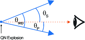
Figure 1: Viewing geometry: Illustration of the velocity vectors of two chunks, the primary chunk at $\theta_{\rm P}$ and the secondary chunk at $\theta_{\rm S}=\theta_{\rm sep.}-\theta_{\rm P}$.

The mass of a typical QN chunk for typical QN parameters is $10^{19}\ {\rm gm}<m_{\rm c}<10^{23}\ {\rm gm}$ depending on whether the QN ejecta breaks up in the solid or liquid phase. In reality, the fragmentation (i.e. the mass of a typical chunk and the resulting number of fragments; whose parameters are hereafter assigned the subscript “c”) is more complicated than the estimates presented in Ouyed, R. & Leahy (2009). For simplicity, we set the number of chunks fixed to $N_{\rm c}=10^{6}$ which implies a typical chunk mass $m_{\rm c}=M_{\rm QN}/N_{\rm c}\simeq 10^{22.5}$ gm; we assume that they all have the same mass (the implications of having a mass distribution are mentioned at the end of §  8.4). The distribution of QN chunks is equally spaced in solid angle and centered on the explosion site (see Figure 1 and Appendix B.1).

2.3.2 Chunk’s maximum size

The very early stages of the evolution of the QN ejecta are dominated by adiabatic losses inducing an almost instantaneous loss of the ejecta’s internal energy; mainly due to the rapid expansion in the degenerate relativistic regime of the ejecta (Ouyed, R. & Leahy 2009). However, re-heating from $\beta$-decay and from sweeping of ambient material (see Appendix B.3) keeps the chunk’s temperature high enough that it will continue to expand until it reaches the transparency radius (when the chunk becomes optically thin). The chunk’s size at transparency, in the co-moving frame where quantities are primed, is given by

$$\kappa_{\rm c}^{\prime}\rho_{\rm c,T}^{\prime}R_{\rm c,T}^{\prime}=1\ .$$ (1)

Here $\kappa_{\rm c}^{\prime}$ is the chunk’s opacity and the subscript “T” stands for “Transparent”. Writing the density as $\rho_{\rm c,T}^{\prime}=m_{\rm c}/(A_{\rm c,T}^{\prime}R_{\rm c,T}^{\prime})$ yields a critical cross-section area

$$A_{\rm c,T}=A_{\rm c,T}^{\prime}\sim 2.4\times 10^{21}\ {\rm cm}^{2}\times m_{\rm c,22.5}\kappa_{\rm c,-1}\ ,$$ (2)

or a radius of $R_{\rm c,T}^{\prime}\sim 2.8\times 10^{10}\ {\rm cm}^{2}\times m_{\rm c,22.5}^{1/2}\kappa_{\rm c,-1}^{1/2}$. When the chunk hits this critical size it stops expanding. The un-primed cross-section area is in the NS frame of reference (i.e. the GRB cosmological rest frame; see Appendix A for the different reference frames involved here). We take a typical chunk’s opacity to be $\kappa_{\rm c}=0.1$ cm² g^-1 (see Appendix B.2); $\kappa_{\rm c}^{\prime}=\kappa_{\rm c}$ since opacity is frame independent.

The corresponding baryon number density, $\frac{m_{\rm c}/m_{\rm H}}{(4\pi/3){R_{\rm c,T}^{\prime}}^{3}}$, in the chunk’s frame is

$$n_{\rm c,T}^{\prime}\sim 2.2\times 10^{14}\ {\rm cm}^{-3}\times m_{\rm c,22.5}^{-1/2}\times\kappa_{\rm c,-1}^{-3/2}\ .$$ (3)

2.3.3 The chunk’s sweeping luminosity

As it sweeps up protons and electrons from the ambient medium of baryon number density $n_{\rm amb.}$, the chunk gains energy which it emits as radiation. The evolution of the chunk’s sweeping luminosity $L_{\rm c,sw.}^{\prime}(t^{\prime})$ and its Lorentz factor $\Gamma_{\rm c}(t^{\prime})$ are given by Eqs. (5) and (6) in Appendix B.3. When the chunk is coasting at its maximum, constant size, given by $A_{\rm c,T}\propto m_{\rm c}$, then the chunk’s mass cancels out of Eq. (6). This implies that the time evolution of the chunk’s Lorentz factor $\Gamma_{\rm c}(t^{\prime})$ is determined by the ambient density alone $\rho_{\rm amb.}=\mu_{\rm H}m_{\rm H}n_{\rm amb.}$; we take a mean molecular weight of $\mu_{\rm H}=1.25$ with $m_{\rm H}$ the hydrogen mass. Equations (5) and (6) can be integrated to yield the evolution of the chunk’s Lorentz factor and the resulting, promptly radiated, sweeping luminosity:

$$\Gamma_{\rm c}(t^{\prime}) =\frac{\Gamma_{\rm QN}}{\left(1+\frac{t^{\prime}}{t_{\Gamma}^{\prime}}\right)^{1/2}}$$ (4)

$$L_{\rm c,sw.}^{\prime}(t^{\prime}) =1.1\times 10^{36}\ {\rm erg\ s}^{-1}\times$$ (5)

$$\times m_{\rm c,22.5}\kappa_{\rm c,-1}n_{\rm amb.,0}\Gamma_{\rm c,3.5}(t^{\prime})^{2}\ ,$$

with $\Gamma_{\rm c}(0)=\Gamma_{\rm QN}$. The chunk’s Lorentz factor decreases after a characteristic hydrodynamical timescale (taking $\beta_{\rm c}=v_{\rm c}/c=1$ where $c$ is the speed of light):

$$t_{\Gamma}^{\prime}\simeq\frac{9.9\times 10^{6}\ {\rm s}}{n_{\rm amb.,0}\Gamma_{\rm QN,3.5}^{2}\kappa_{\rm c,-1}}\ ,$$ (6)

which is effectively set by the ambient density for a given QN explosion; i.e. for a given $\Gamma_{\rm QN}$. The equations above assumes a constant ambient density. In the case of varying ambient density, Eq.(5) still holds but Eq.(4) must be replaced by re-integrating Eq.(6) accordingly.

3 A QN in the wake of a SN

We now consider a QN occurring after a SN explosion in which a rapidly rotating NS was born with a mass above the critical mass $M_{\rm NS,cr.}$. For such NSs, the increase in core density is most dramatic at $t_{\rm SpD}$, the spin-down characteristic timescale (see Staff et al. 2006). In other words, it is natural to assume that the time-delay $t_{\rm QN}$ between the SN proper and the exploding neutron star is the spin-down timescale; i.e. $t_{\rm QN}\simeq t_{\rm SpD}$ when $M_{\rm NS}\geq M_{\rm NS,c.}$. Hereafter, we keep fixed the radius and mass of the NS and set them to $R_{\rm NS}=10$ km and $M_{\rm NS}=M_{\rm NS,cr.}=2M_{\odot}$, respectively. The NS moment of inertia we take to be $I_{\rm NS}=10^{45}$ g cm².

The decline of the pulsar spin-down power, assuming a magnetic dipole, depends on time as (Deutsch 1955; Manchester & Taylor 1977),

$$L_{\rm SpD}(t)=L_{\rm SpD,0}\left(1+\frac{t}{t_{\rm SpD}}\right)^{-2}\ ,$$ (7)

with

$$L_{\rm SpD,0}\simeq 3.9\times 10^{41}\ {\rm erg\ s}^{-1}\times P_{\rm NS,-2.4}^{-4}B_{\rm NS,12.5}^{2}\ ,$$ (8)

$$t_{\rm SpD}\simeq 103.7\ {\rm years}\times P_{\rm NS,-2.4}^{2}B_{NS,12.5}^{-2}\ ,$$ (9)

and a rotational energy, $E_{\rm SpD}=(1/2)I_{\rm NS}(2\pi/P_{\rm NS})^{2}$, of

$$E_{\rm SpD}\simeq 1.2\times 10^{51}\ {\rm erg}\times P_{\rm NS,-2.4}^{-2}\ .$$ (10)

The subscript “SpD” stands for spin-down. The NS’s birth period and magnetic field are given in units of 4 milliseconds ($P_{\rm NS,-2.4}=P_{\rm NS}/4$ ms) and $10^{12.5}$ G ($B_{\rm NS,12.5}=B_{\rm NS}/10^{12.5}$ G), respectively (hereafter our fiducial values).

3.1 Summary of model’s parameters

The parameters described below are in chronological order starting with the SN, followed by the Pulsar Wind Nebula (PWN) phase describing the interaction between the SN ejecta and the PW and, the QN proper which occurs at time $t_{\rm QN}=t_{\rm SpD}$ following the SN.

• SN parameters: There are 5 parameters. The first 3 are the SN ejecta’s kinetic energy $E_{\rm SN}$, the SN ejecta’s mass $M_{\rm SN}$ and $n$ which is the power-law index of the SN’s steep density part overlaying the density plateau. We set the SN fiducial values as $E_{\rm SN}=10^{51}\ {\rm erg}$, $M_{\rm SN}=10^{34}$ grams (i.e. $5M_{\odot}$) and $n=9$.

  The SN ambient medium the SN explodes into is defined by its baryon number density $n_{\rm amb.}$ and magnetic field $B_{\rm amb.}$. We list them as part of the SN parameter set with fiducial values of 1 cm^-3 and $10^{-5}$ G.

• NS parameters: With the radius and mass of the NS set to $10$ km and $2M_{\odot}$, respectively, there are only 2 free parameters which are the NS’s birth period $P_{\rm NS}$ and birth magnetic field $B_{\rm NS}$. The birth period varies only by a factor of a few from one SN to another since only massive NSs with spin period $P_{\rm NS}$ of a few milliseconds can experience substantial increase in their core’s density and explode as QNe (Staff et al. 2006). For $B_{\rm NS}$, we take a log-normal distribution with mean $12.5$ and variance $\sigma_{\rm\log B}=0.5$ (e.g. Faucher-Giguère & Kaspi 2006 and references therein).

  The range in $t_{\rm SpD}$ is controlled by the NS birth magnetic field $B_{\rm NS}$ which varies by orders of magnitude from one source to another unlike $P_{\rm NS}$ which varies by a factor of a few at most.

• QN parameters: There are 4 parameters. The first 2 parameters are the ejecta’s kinetic energy $E_{\rm QN}=10^{53}$ ergs (kept fixed; effectively set by the NS mass $M_{\rm NS,c.}$), and its Lorentz factor $\Gamma_{\rm QN}=10^{3.5}$ also kept fixed. The ejecta’s mass is then given by $M_{\rm QN}=E_{\rm QN}/\Gamma_{\rm QN}c^{2}\sim 10^{-4.75}M_{\odot}$ (representative of the NS’s outermost crust). The third parameter we take to be the total number of chunks $N_{\rm c}=10^{6}$ which yields a typical QN chunk’s mass $m_{\rm c}=10^{22.5}$ gm. Other parameters/properties of the QN ejecta such as the chunk’s critical cross-section area $A_{\rm c,T}$ and the corresponding rest-frame baryon number density $n_{\rm c,T}^{\prime}$ (given by Eqs. (2) and (3), respectively) are all known once the mass of the chunk is known.

Table 1 lists the fiducial values for our parameters. The SN and NS parameters combined yield the properties of the PWN-SN turbulent shell (resulting from the interaction between the PWN and the SN ejecta) which we refer to as the “wall”.

3.2 The SN ejecta

We describe the SN ejecta and how it is shaped by its interaction with the underlying PWN and with the overlaying ambient medium (with constant baryon number density $n_{\rm amb.}$ and magnetic field $B_{\rm amb.}$) prior to the QN event.

The analytical SN and PWN models we adopt here are the self-similar solutions given in Chevalier (1977, 1982, 1984); Blondin et al. (1998, 2001); see also Reynolds & Chevalier 1984; van der Swaluw et al. 2001, 2003, 2004; Chevalier 2005. For a constant $n_{\rm amb.}$, the size of the SN ejecta is given by $R_{\rm SN}=\alpha_{\rm n}(Av_{\rm t}^{n}/\rho_{\rm amb.})^{1/n}t^{(n-3)/n}$ with $A=((5n-25)/(2\pi n))\times E_{\rm SN}v_{\rm t}^{-5}$ and $v_{\rm t}=((10n-50)/(3n-9)\times E_{\rm SN}/M_{\rm SN})^{1/2}$ is the velocity at the intersection between the density plateau of the SN ejecta. The SN ejecta’s power law steep density gradient is set by the parameter $n$. For $n=9$, $\alpha_{9}=1.048$, $A=1.5\times 10^{7}$ g cm^-3 s${}^{3}\times{E_{\rm SN,51}}^{-3/2}M_{\rm SN,34}^{5/2}$ and $v_{\rm t}=4.7\times 10^{3}$ km s${}^{-1}\times{E_{\rm SN,51}}^{1/2}M_{\rm SN,34}^{-1/2}$. I.e.

$$R_{\rm SN}(t)\simeq 3.0\times 10^{18}\ {\rm cm}\times\left({E_{\rm SN,51}}^{1/3}M_{\rm SN,34}^{-2/9}n_{\rm amb.,0}^{-1/9}\right)\times t_{9.5}^{2/3}\ .$$ (11)

Since $t_{\rm QN}=t_{\rm SpD}\sim 100$ years for our fiducial values, the time-dependency of the SN properties are given in units of $100$ years; i.e. $t_{9.5}=t/(10^{9.5}\ {\rm s})=t/(100\ {\rm years})$.

The SN ejecta’s density profile is

$$\rho_{\rm SN}(r,t)=\begin{cases}\rho_{\rm Plat.}(t),&\text{for\ }r<R_{\rm Plat.}\\ \rho_{\rm Plat.}(t)\times\left(\frac{R_{\rm Plat.}}{r}\right)^{-n},&\text{for\ }r>R_{\rm Plat.}\end{cases}$$ (12)

with $R_{\rm Plat.}(t)=v_{\rm t}t$ defines the edge of the density plateau in the inner SN ejecta and $\rho_{\rm Plat.}(t)=At^{-3}$ is the time-evolving plateau’s density.

For our fiducial SN parameters, we get

$$R_{\rm Plat.}(t)\simeq 1.5\times 10^{18}\ {\rm cm}\times\left({E_{\rm SN,51}}^{1/2}M_{\rm SN,34}^{-1/2}\right)\times t_{9.5}\ ,$$ (13)

with the plateau’s baryon number density, $n_{\rm Plat.}(t)=\rho_{\rm Plat.}(t)/m_{\rm H}$, being

$$n_{\rm Plat.}(t)\simeq 2.9\times 10^{2}\ {\rm cm}^{-3}\times\left({E_{\rm SN,51}}^{-3/2}M_{\rm SN,34}^{5/2}\right)\times t_{9.5}^{-3}\ .$$ (14)

3.3 The PWN-SN shell: the “wall”

The collision between the PWN and the inner SN ejecta (the plateau) leads to the formation of an PWN-SN dense shell (i.e. the “wall” with its parameters denoted with subscript “w”). The wall is at a radius $R_{\rm w}=1.5\left(\frac{n}{n-5}\right)^{1/5}\left(\frac{n-5}{n-3}\right)^{1/2}\left(\frac{{E_{\rm SN}}^{3}L_{\rm SpD}^{2}}{M_{\rm SN}^{5}}\right)^{1/10}t^{6/5}$ or,

$$R_{\rm w}(t) \sim 1.5\times 10^{18}\ {\rm cm}~{}\times$$ (15)

$$\times\left(\frac{{E_{\rm SN,51}}^{3}}{M_{\rm SN,34}^{5}}\right)^{1/10}\left(\frac{P_{\rm NS,-2.4}^{-2}}{t_{\rm SpD,100}}\right)^{1/5}\times t_{9.5}^{6/5}\ ,$$

which assumes a constant pulsar luminosity $L_{\rm SpD}=E_{\rm SpD}/t_{\rm SpD}$. The corresponding wall’s speed, $V_{\rm w}=dR_{\rm w}/dt=R_{\rm w}/t\propto t^{1/5}$, is

$$V_{\rm w}(t) \sim 5.7\times 10^{3}\ {\rm km\ s}^{-1}\times$$ (16)

$$\times\left(\frac{{E_{\rm SN,51}}^{3}}{M_{\rm SN,34}^{5}}\right)^{1/10}\left(\frac{P_{\rm NS,-2.4}^{-2}}{t_{\rm SpD,100}}\right)^{1/5}\times t_{9.5}^{1/5}\ .$$

For $t=t_{\rm QN}=t_{\rm SpD}$, we have $V_{\rm w}\propto P_{\rm NS}^{-2/5}$. I.e. the wall’s speed varies very little in time and is roughly constant from one source to another in our model.

The wall’s baryon number density is $n_{\rm w}=f_{\gamma_{\rm ad.}}\times(\rho_{\rm SN}/m_{\rm H})$ with $\rho_{\rm SN}/m_{\rm H}$ is the SN ejecta’s baryon number density and $f_{\gamma_{\rm ad.}}=(\gamma_{\rm ad.}+1)/(\gamma_{\rm ad.}-1)$ is the shock compression factor set by the adiabatic index $\gamma_{\rm ad.}$. This gives, for $\gamma_{\rm ad.}=5/3$,

$$n_{\rm w}(t)\sim 1.2\times 10^{3}\ {\rm cm}^{-3}\times\left({E_{\rm SN,51}}^{-3/2}M_{\rm SN,34}^{5/2}\right)\times t_{9.5}^{-3}\ .$$ (17)

The maximum wall’s thickness can roughly be estimated from mass conservation to be $\Delta R_{\rm w}/R_{\rm w}=1/(3f_{\gamma_{\rm ad.}})$ so that $\Delta R_{\rm w}/R_{\rm w}=1/12$. In principle, the wall can be thinner if cooling is taken into account.

3.3.1 The wall’s magnetic field

The development of the Rayleigh-Taylor (RT) instability within the PWN-SN interface (e.g. Chevalier & Klein 1978) means that the wall’s magnetic field is prone to turbulent amplification (e.g. Jun et al. 1995; Jun 1998; Bucciantini et al. 2004; Duffell & Kasen 2017; see also Stone & Gardiner 2007; Porth et al. 2014). These studies find that the amplified magnetic field can be estimated using equipartition arguments which allows us to assume for simplicity that $B_{\rm w}^{2}/8\pi=\epsilon_{\rm w}\times n_{\rm w}k_{\rm B}T_{\rm w,sh.}$ where the shocked wall temperature is given by $k_{\rm B}T_{\rm w,sh.}=3/16\times\mu_{\rm e}m_{\rm H}V_{\rm w}^{2}$ and $\epsilon_{\rm w}$ being the ratio of magnetic to thermal energy at the PWN-SN shock. We take the mean molecular weight per electron to be $\mu_{\rm e}=2$ representative of the type-Ic SN ejecta. This yields

$$B_{\rm w}(t)\simeq 0.8\ {\rm mG}\ \times\epsilon_{\rm w,-5}^{1/2}n_{\rm w,3}(t)^{1/2}V_{\rm w,8.7}(t)\ ,$$ (18)

where we set $\epsilon_{\rm w}=10^{-5}$ as our fiducial value since it gives milli-Gauss values in line with simulations and measurements of the magnetic field strength in SNRs (e.g. Reynolds et al. 2012 and references therein). This parameter enters when calculating the spectrum (i.e. the synchrotron emission) and is thus listed in Table 1. Since $V_{\rm w}$ (given in units of $10^{8.7}$ cm s^-1= 5000 km s^-1) varies little from one source to another (see Eq. (16)), the wall’s magnetic field depends essentially on the wall’s density and the strength of the turbulent amplification parameter $\epsilon_{\rm w}$. However, since $\epsilon_{\rm w}$ is expected to be constant once turbulence saturation is reached in the PWN-SN ejecta this leaves $n_{\rm w}$ as the controlling parameter.

Table 1: Fiducial parameters in our model (see §  3.1).

SN					NS		QN			Spectrum (see § 4.2.5)
$E_{\rm SN}$	$M_{\rm SN}$	$n$	$n_{\rm amb.}$	$B_{\rm amb.}$	$P_{\rm NS}$	$B_{\rm NS}^{\mathbf{a}}$	$E_{\rm QN}$	$\Gamma_{\rm QN}$	$N_{\rm c}$	$\epsilon_{\rm w}^{\mathbf{b}}$	$p$	$n_{\rm pairs}$
$10^{51}$ erg	$10^{34}\ {\rm gm}$ ($=5M_{\odot}$)	9	1 cm-3	$10^{-5}$ G	$10^{-2.4}$ s (= 4 ms)	$10^{12.5}$ G	$10^{53}$ erg	$10^{3.5}$	$10^{6}$	$10^{-5}$	2.4	10

^a We adopt a log-normal distribution for the magnetic field with mean $10^{12.5}$ G and variance $\sigma_{\rm\log B}=0.5$ (see §  3.1).
^b The wall’s magnetization factor as defined in Eq. (18).

3.4 Characteristic timescales

There are two critical timescales that define the interaction between the PW and the SN ejecta (e.g. Blondin et al. 2001; Chevalier 2005), prior to the QN explosion:

• The SN density plateau: The wall would reach the edge of the SN ejecta plateau at time (obtained by equating Eqs. (15) and (13))

  $$t_{\rm Plat.}\sim\left(\frac{E_{\rm SN}}{E_{\rm SpD}}\right)t_{\rm SpD}\ ,$$ (19)

  in the constant spin-down luminosity case. The condition $t_{\rm QN}=t_{\rm SpD}>t_{\rm Plat.}$ is satisfied whenever $E_{\rm SN}\leq E_{\rm SpD}$ and is equivalent to

  $$P_{\rm NS}\leq P_{\rm NS,cr.}\sim\frac{4\ {\rm ms}}{{E_{\rm SN,51}}^{1/2}}\ \cdot$$ (20)

  For $P_{\rm NS}<P_{\rm NS,cr.}$ (i.e. when $t_{\rm Plat.}<t_{\rm SpD}$), the QN occurs after the wall has reached the edge of the density plateau. I.e., the SN ejecta is already blown-out by the PWN (see Figure 6 in Blondin & Chevalier (2017)) and can no longer be described by a self-similar solution. This case is more relevant in our model since it gives best fits to light-curves and spectra of observed LGRBs as we show in §  5.3. Thus for our fiducial values, the blow-out regime corresponds to NSs born with a period in the range $1.5\ {\rm ms}<P_{\rm NS}\leq P_{\rm NS,cr.}$ with the lower limit set by the r-mode instability on rapidly rotating accreting NS (Andersson et al. 1999, 2000);

• The SN reverse shock: When the SN reverse shock (RS) propagates inward to the edge of the SN plateau it triggers its inward motion and eventually “crushes” the PWN. The relevant timescale for $n=9$ is

  $$t_{\rm SN,RS}\simeq 459\ {\rm years}\times{E_{\rm SN,51}}^{-1/2}M_{\rm SN,34}^{5/6}n_{\rm amb.,0}^{-1/3}\ .$$ (21)

  For the constant pulsar luminosity case, the ratio between the pressure in the PWN and behind the RS can be estimated (e.g. Eq. (9) in Blondin et al. 2001; see also van der Swaluw et al. 2001) to be $P_{\rm PWN}/P_{\rm RS}\sim 1.5$ for our fiducial values. Thus, no crushing is more likely. Nevertheless, we impose $t_{\rm SpD}<t_{\rm SN,RS}$ (which guarantees $t_{\rm Plat.}<t_{\rm SN,RS}$ because $t_{\rm Plat.}<t_{\rm SpD}$). This means we do not need to consider the effect of the SN reverse shock on the PWN. We cannot rule out the scenario where the QN occurs while the wall has been crushed to smaller radii. However, the evolution of the crushed PWN changes so that the current model is not applicable. This is a complication beyond the scope of this paper and may be worth exploring elsewhere.

Other timescales relevant to our model:

• The SN optical depth $\tau_{\rm SN}$: The conditions $\tau_{\rm SN}<1$ (i.e. an optically thin SN; see Appendix C), translates to

  $$t_{\rm QN}>t_{\rm SLSN}\sim 1.8\ {\rm years}\times{E_{\rm SN,51}}^{-1/2}M_{\rm SN,34}\ .$$ (22)

  For $\tau_{\rm SN}>1$, the QN kinetic energy is “absorbed” in the SN envelope re-brightening the SN and yielding a SLSN (see §  5.4.1);

In summary, the range in time delay between the SN and the QN applicable to GRBs is $t_{\rm SLSN}<t_{\rm QN}=t_{\rm SpD}<t_{\rm SN,RS}$ which for our fiducial values gives

$$1.8\ {\rm yr}<t_{\rm QN}<460\ {\rm yr}\ .$$ (23)

The corresponding range in wall’s density (which controls the GRB luminosity in our model) can be derived by incorporating the range in $t_{\rm QN}$ given in Eq. (23) into Eq. (17) to get

$$12.6\ {\rm cm}^{-3}<n_{\rm w}<2.1\times 10^{8}\ {\rm cm}^{-3}\ .$$ (24)

The corresponding wall’s size (which controls GRB timescales in our model) is derived by incorporating the range in $t_{\rm QN}$ in Eq. (23) into Eq. (15) to get

$$1.2\times 10^{16}\ {\rm cm}<R_{\rm w}<9.3\times 10^{18}\ {\rm cm}\ .$$ (25)

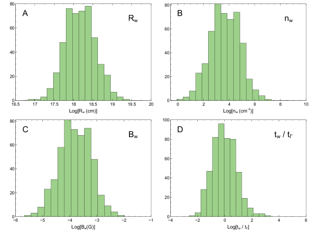
Figure 2: PWN-SN shell (“the wall”) properties: Distributions of the wall’s parameters (radius $R_{\rm w}$, density $n_{\rm w}$, magnetic field $B_{\rm w}$ and thickness parameter $t_{\rm w}/t_{\Gamma}$) for a distribution of $t_{\rm QN}$ (i.e. $B_{\rm NS}$) in our model. We use Rice’s rule for binning

The first 3 panels in Figure 2 show the $n_{\rm w},R_{\rm w}$ and $B_{\rm w}$ distributions, for our fiducial values of parameters, applicable to GRBs. The time delay, $t_{\rm QN}=t_{\rm SpD}$, is set by drawing $B_{\rm NS}$ from a log-normal distribution with mean of 12.5 and a variance $\sigma_{\rm\log B_{\rm NS}}=0.5$ (see Table 1).

4 Application to long duration GRBs I: A non-turbulent PWN-SN ejecta

In this proof-of-principle section, we present the simple but analytically tractable case of: (i) the QN chunks colliding with a non-turbulent self-similar PWN-SN shell (i.e. the wall as described above) located at $R_{\rm w}$ (with thickness $\Delta R_{\rm w}=R_{\rm w}/12$), density $n_{\rm w}$ and magnetic field $B_{\rm w}$; (ii) $t_{\rm QN}=t_{\rm SpD}$ which gives, for the fiducial values of our parameters, $t_{\rm QN}\sim 100$ years, $n_{\rm w}\sim 10^{3}$ cm^-3, $R_{\rm w}\sim 10^{18}$ cm and $B_{\rm w}\sim$ mG.

Once the NS explodes, the QN ejecta is ultra-relativistic. It catches up with the wall in less than a year during which time we assume the wall properties did not evolve. There are 3 distinct regions the QN ejecta interacts with: (i) the pre-wall phase (the inside of the PWN) before they collide with the wall; (ii) the wall phase (giving us the prompt emission and the GRB proper); (iii) the post-wall phase when the chunks interact with the ambient medium (giving us the afterglow).

This simple case will be used later as a reference when applying our model to the fully turbulent PWN-SN shell in the blow-out regime (i.e. for $E_{\rm SN}<E_{\rm SpD}$; see Eq. (19)) which is relevant to most LGRBs (see §  5.3).

4.1 The pre-wall phase: QN chunks inside the PWN

Inside the PW bubble (see Appendix B.4) the density is low enough that a chunk’s sweeping luminosity (Eq. (5)) is dwarfed by heating from the $\beta$-decay of r-process elements in the chunk; i.e. $L_{\rm c,sw.}^{\prime}(t^{\prime})<<L_{\rm c,\beta}^{\prime}(t^{\prime})$ with the $\beta$-decay power given by Eq. (4). The time evolution of the chunk’s temperature $T_{\rm c}^{\prime}(t^{\prime})$ and cross-section area $A_{\rm c}^{\prime}(t^{\prime})$ during the optically thick regime (i.e. before transparency) is found from Eqs. (10) and (11), respectively, in Appendix B.4.

The distance travelled by a chunk in the NS frame before it becomes optically thin is $R_{\rm T}$ given by Eq. (13) which, within a factor of a few, is close to $R_{\rm w}$. The chunk’s temperature in the pre-wall phase at transparency (i.e. the corresponding blackbody at $t_{\rm T}^{\prime}$ found from $A_{\rm c,T}\sigma_{\rm SB}{T_{\rm c,T}^{\prime}}^{4}=L_{\rm c,\beta}(t^{\prime})$) is

$$k_{\rm B}T_{\rm c,T}^{\prime}\simeq 0.23\ {\rm eV}\times m_{\rm c,22.5}^{-0.194}\kappa_{c,-1}^{-3.3/6.7}\ .$$ (26)

Thus, in the non-turbulent PWN-SN shell (i.e. the single wall) scenario, we have the simple picture of the chunks being cool and optically thin when they start colliding with the wall.

4.2 The wall phase: QN chunks inside the wall

Important properties:

• Doppler effects: Appendix A lists the references frames in our model: the chunk’s frame (primed quantities), the NS frame (unprimed quantities) and the observer’s frame (quantities with superscript “obs.”). Since $\Gamma_{\rm c}(t^{\prime})^{2}>>1$ and $\theta_{\rm c}<<1$ applies we can write the Doppler factor as $D_{\rm c}(\Gamma_{\rm c}(t^{\prime}),\theta_{\rm c})\simeq 2\Gamma_{\rm c}(t^{\prime})/(1+\Gamma_{\rm c}(t^{\prime})^{2}\theta_{\rm c}^{2})$;

• The primary chunk at $\theta_{\rm P}$ (closest to the line-of-sight) causes the prompt and afterglow emission: Figure 1 shows the spacing between the QN chunks as presented in Appendix B.1. The distribution of QN chunks is equally spaced in solid angle and centered on the explosion site. Because the angular spacing between chunks is several times larger than $1/\Gamma_{\rm c}\sim 3.2\times 10^{-4}/\Gamma_{\rm c,3.5}$, there will almost always be a single chunk dominating the observed prompt emission. This chunk we refer to as the “primary” chunk and is depicted with subscript “P”. The primary’s viewing angle is $0<\theta_{\rm P}<2\times 10^{-3}/N_{\rm c,6}^{1/2}$ with an average value $\bar{\theta}_{\rm P}\sim(4/3)/N_{\rm c}^{1/2}\simeq 1.3\times 10^{-3}/N_{\rm c,6}^{1/2}$;

• The secondary chunk at $\theta_{\rm S}$ causes the flares: Each primary chunk is surrounded by about 6 peripheral chunks (the secondaries) as described in Figure 1 with $\theta_{\rm S}=\theta_{\rm sep.}-\theta_{\rm P}=4/N_{\rm c}^{1/2}-\theta_{\rm P}$; $\theta_{\rm sep.}=4/N_{\rm c}^{1/2}$ is the separation between adjacent chunks. Hereafter we use the simplification that these secondary chunks are combined into a single chunk whose viewing angle is in the range $2\times 10^{-3}/N_{\rm c,6}^{1/2}<\theta_{\rm S}<4\times 10^{-3}/N_{\rm c,6}^{1/2}$ with an average value $\bar{\theta}_{\rm S}=(28/9)/N_{\rm c}^{1/2}\simeq 3.1\times 10^{-3}/N_{\rm c,6}^{1/2}$. The secondary chunk defines the flaring activity in our model and acts as a repeat, or echo, of the prompt GRB induced by the primary chunk;

• The chunk’s forward shock (FS) and reverse shock (RS): The QN chunk collision with the wall yields a FS and a RS. The RS is relativistic when $n_{\rm c}^{\prime}/n_{\rm w}<<\Gamma_{\rm QN}^{2}$, (e.g. Landau & Lifschitz 1959; Blandford & McKee 1976; Mésźaros & Rees 1992; Sari & Piran 1995). This case implies that most of the chunk’s kinetic energy is converted to internal energy, slowing down the chunk in a fraction of a second (the time it takes the RS to cross the chunk). Using Eq. (3) for $n_{\rm c}^{\prime}$, this occurs when

  $$n_{\rm w}>n_{\rm w,RS}=2.2\times 10^{7}\ {\rm cm}^{-3}\times\left(m_{\rm c,22.5}^{-1/2}\kappa_{\rm c,-1}^{-3/2}\Gamma_{\rm c,3.5}^{-2}\right)\ .$$ (27)

  Using Eq. (17) this happens when

  $$t_{\rm QN}<t_{\rm QN,RS} =3.8\ {\rm yrs}\times\left(E_{\rm SN,51}^{-1/2}M_{\rm SN,34}^{5/6}\right)\times$$ (28)

  $$\times\left(m_{\rm c,22.5}^{1/6}\kappa_{\rm c,-1}^{1/2}\Gamma_{\rm c,3.5}^{2/3}\right)\ .$$

  The above is for $n_{\rm w}=f_{\gamma_{\rm ad.}}n_{\rm Plat.}=4n_{\rm Plat.}$. For higher compression factor $f_{\gamma_{\rm ad.}}$, $t_{\rm QN,RS}$ is higher by a multiplicative factor $(f_{\gamma_{\rm ad.}}/4)^{1/3}$.

  For $t_{\rm QN,RS}<t_{\rm QN}<t_{\rm SN,RS}$, the chunk’s RS is Newtonian. In this case, the dynamics and the emission is dominated by the FS which moves with a Lorentz factor $\Gamma_{\rm FS}(t^{\prime})$;

• The wall’s (i.e. PWN-SN shell) geometry: We assume that the wall is perfectly aligned along a spherical shell centered on the QN explosion. In addition we assume that the wall is continuous spatially, and has a uniform density $n_{\rm w}$;

• The relevant timescales: There are two contributions: (i) a radial time delay which arises as the primary chunk crosses the wall and; (ii) an angular time delay between the primary chunk hitting at $\theta_{\rm P}$ and the secondary chunk hitting the wall at a higher viewing angle $\theta_{\rm S}$. The angular time delay between them is

  $$\Delta t_{\rm S-P}=\frac{R_{\rm w}\theta_{\rm S}^{2}}{2c}-\frac{R_{\rm w}\theta_{\rm P}^{2}}{2c}\ .$$ (29)

  The component which dominates the GRB duration enters later when we consider a turbulent PWN-SN ejecta is the radial time delay which takes into account the radial distribution and extent of multiple filaments from the “shredded” wall (see §  5.3);

• The thin and thick wall scenarios: Let us define $t_{\rm w}^{\prime}=\Delta R_{\rm w}/\Gamma_{\rm FS}c$ as a measure of the wall’s crossing time in the chunk’s frame with $\Delta R_{\rm w}=R_{\rm w}/12$ the wall’s thickness in the NS frame. The distribution of the thickness parameter $t_{\rm w}^{\prime}/t_{\Gamma}^{\prime}=t_{\rm w}/t_{\Gamma}$ is shown in the lower right panel in Figure 2 for fiducial values of our parameters. If $t_{\rm w}^{\prime}<t_{\Gamma}^{\prime}$ then the chunks will wall experience no deceleration (thin wall case) while in the thick wall case ($t_{\rm w}^{\prime}>t_{\Gamma}^{\prime}$ ) there is significant deceleration on timescales of a few times $t_{\Gamma}^{\prime}$.

In the remainder of this section, we use the thin wall case (i.e. $t_{\rm w}^{\prime}<3t_{\Gamma}^{\prime}$) where the chunk’s Lorentz factor remains roughly constant when crossing the wall so we can write $\Gamma_{\rm FS}(t^{\prime})\simeq\Gamma_{\rm QN}=10^{3.5}$. The thick wall case (with $t_{\rm w}^{\prime}>3t_{\Gamma}^{\prime}$) is presented in Appendix D and is compared to the thin wall case at the end of this section.

It is useful to differentiate between the 3 sets of parameters: (i) the wall (i.e. PWN-SN shell) parameters; (ii) the chunk/QN parameters; (iii) the observer’s parameters mainly defined by the viewing angle $\theta_{\rm c}$. For the solutions presented in what follows we only vary the viewing angles $\theta_{\rm P}$ and $\theta_{\rm S}$ and the time delay between the QN and SN, $t_{\rm QN}=t_{\rm SpD}$. In the thin wall case, the Doppler factor depends only on the viewing angle so that that $D(\Gamma_{\rm c}(t^{\prime}),\theta_{\rm c})\simeq D(\Gamma_{\rm QN},\theta_{\rm c})=2\Gamma_{\rm QN}/f(\theta_{\rm c})$ with

$$f(\theta_{\rm c})=1+(\Gamma_{\rm QN}\theta_{\rm c})^{2}\ .$$ (30)

For $0<\theta_{\rm c}=\theta_{\rm P}<2\times 10^{-3}/N_{\rm c,6}^{1/2}$ this implies $0\leq f(\theta_{\rm P})\leq 41$ and $f(\bar{\theta}_{\rm P})\simeq 17.9$ for the primary chunk. For the secondary chunk we have $2\times 10^{-3}/N_{\rm c,6}^{1/2}<\theta_{\rm c}=\theta_{\rm S}<4\times 10^{-3}/N_{\rm c,6}^{1/2}$ with a corresponding $41\leq f(\theta_{\rm S})\leq 161$ and $f(\bar{\theta}_{\rm S})\simeq 97.1$.

Hereafter, we will refer to the prompt emission (induced by the primary chunk) by the subscript “GRB”, the flaring (induced by the secondary chunk) by the subscript “Flare” and the afterglow (induced by the primary chunk) by the subscript “AG”, respectively.

4.2.1 The luminosity

When $t_{\rm QN,RS}<t_{\rm QN}<t_{\rm SN,RS}$, the RS into the chunk is purely Newtonian. The emission is dominated by the chunk’s FS moving at a Lorentz factor $\Gamma_{\rm FS}\simeq\Gamma_{\rm QN}$. The observed luminosity from a single chunk seen at an angle $\theta_{\rm c}=\theta_{\rm P}$ from the line-of-sight hitting the wall of density $n_{\rm w}$ is $L_{\rm GRB}=D(\Gamma_{\rm QN},\theta_{\rm P})^{4}L_{\rm c,sw.}^{\prime}$ where the chunk’s sweeping luminosity $L_{\rm c,sw.}^{\prime}(t^{\prime})$ is given by Eq. (5); emitted as synchrotron radiation (see §  4.2.5). This gives

$$L_{\rm GRB} \simeq\left(\frac{1.7\times 10^{54}\ {\rm erg\ s}^{-1}}{f(\theta_{\rm p})^{4}}\right)\times$$ (31)

$$\times(m_{\rm c,22.5}\kappa_{\rm c,-1}\Gamma_{\rm QN,3.5}^{6})\times\left(n_{\rm w,3}\right)\ .$$

With $0<\theta_{\rm P}<2/N_{\rm c}^{1/2}$ and for the range in $n_{\rm w}$ given in Eq. (24) we get

$$7.5\times 10^{45}\ {\rm erg\ s}^{-1}<L_{\rm GRB}<3.5\times 10^{59}\ {\rm erg\ s}^{-1}\ ,$$ (32)

with an average value of $8.8\times 10^{48}\ {\rm erg\ s}^{-1}$.

4.2.2 The duration

The observed duration of emission from a single chunk going through the wall of thickness $\Delta R_{\rm w}$ is $\Delta t_{\rm GRB}=\Delta R_{\rm w}/(D(\Gamma_{\rm QN},\theta_{\rm P})\Gamma_{\rm QN}c)=f(\theta_{\rm P})\times\Delta R_{\rm w}/(2\Gamma_{\rm QN}^{2}c)$. For $\Delta R_{\rm w}/R_{\rm w}=1/12$, we get

$$\Delta t_{\rm GRB}\sim\left(\frac{1}{6}\ {\rm s}\times f(\theta_{\rm P})\right)\times\frac{(R_{\rm w,18})}{(\Gamma_{\rm QN,3.5}^{2})}\ .$$ (33)

For $0<\theta_{\rm P}<2/N_{\rm c}^{1/2}$ and for the range of $R_{\rm w}$ given in Eq. (25) we arrive at

$$4.8\ {\rm ms}<\Delta t_{\rm GRB}<63.6\ {\rm s}\ ,$$ (34)

with an average value of 3 seconds.

4.2.3 The isotropic energy

The isotropic energy ($E_{\rm GRB}=L_{\rm GRB}\Delta t_{\rm GRB}$) is

$$E_{\rm GRB}\simeq\left(\frac{2.8\times 10^{53}\ {\rm erg}}{f(\theta_{\rm p})^{3}}\right)\times$$ (35)

$$\times\left(m_{\rm c,22.5}\kappa_{\rm c,-1}\Gamma_{\rm QN,3.5}^{4}\right)\times\left(n_{\rm w,3}R_{\rm w,18}\right)\ .$$

With $n_{\rm w,3}R_{\rm w,18}\simeq 2.9\times t_{9.5}^{-9/5}$ (i.e. $0.19<n_{\rm w,3}R_{\rm w,18}<183$), the range in isotropic energy is

$$2.1\times 10^{48}\ {\rm ergs}<E_{\rm GRB}<2.7\times 10^{57}\ {\rm ergs}\ ,$$ (36)

with an average value of $\sim 5\times 10^{49}\ {\rm ergs}$.

4.2.4 The afterglow

Exiting the wall and the SN with a Lorentz factor of $\sim\Gamma_{\rm QN}$, the primary chunk interacts with the surrounding ambient medium (subscript “amb.”) and radiates at a rate of

$$L_{\rm AG} \simeq\left(\frac{1.7\times 10^{51}\ {\rm erg\ s}^{-1}}{f(\theta_{\rm P})^{4}}\right)\times$$ (37)

$$\times(m_{\rm c,22.5}\kappa_{\rm c,-1}\Gamma_{\rm QN,3.5}^{6})\times(n_{\rm amb.,0})\ ,$$

with a corresponding range, due to $\theta_{\rm P}$, of

$$6\times 10^{44}\ {\rm erg\ s}^{-1}<L_{\rm AG}<1.7\times 10^{51}\ {\rm erg\ s}^{-1}\ ,$$ (38)

and an average value of $\sim 1.7\times 10^{46}\ {\rm erg}$ s^-1.

The luminosity ratio between the prompt and afterglow emission is given by the density ratio $n_{\rm w}/n_{\rm amb.}\sim 10^{3}$ in the single wall scenario. However, in order to simultaneously fit the prompt, afterglow and flare emission of observed LGRB light-curves, the density jump alone is not sufficient and a decrease in $\Gamma_{\rm FS}$ prior to exiting the GRB phase is necessary (see §  5.3), which is suggestive of a thick wall. A thick wall is also needed to recover the Band-like spectrum (see §  5.2).

The duration of the afterglow is $t_{\rm AG}=t_{\rm\Gamma,amb.}^{\prime}/D(\Gamma_{\rm QN},\theta_{\rm P})$ where $t_{\rm\Gamma,amb.}^{\prime}$ is the dynamical timescale (see Eq. (6)) in the ambient medium:

$$t_{\rm AG}=1.5\times 10^{3}\ {\rm s}\times\frac{f(\theta_{\rm P})}{n_{\rm amb.,0}\Gamma_{\rm QN,3.5}^{3}\kappa_{\rm c,-1}}\ ,$$ (39)

with a range of $1.3\times 10^{3}\ {\rm s}\leq t_{\rm AG}^{\rm obs.}\leq 6.4\times 10^{4}\ {\rm s}$ and an average value of $\sim 2.7\times 10^{4}\ {\rm s}$.

4.2.5 The spectrum

There are 3 more parameters that define the spectrum. The electron energy distribution with the power-law index $p$, the number of pairs $n_{\rm pairs}$ generated in the chunk’s FS per proton swept-up and, $\epsilon_{\rm w}$ the ratio of magnetic to thermal energy defining the wall’s magnetization (see Eq. (18)). Important effects include:

• Acceleration in the FS: A typical electron (or positron) accelerated by the FS acquires the average Lorentz factor of the electrons distribution $\gamma_{\rm e,av.}=(\zeta_{\rm p}\Gamma_{\rm FS}m_{\rm p}/m_{\rm e})/2n_{\rm pairs}$ (e.g. Piran 1999; recall that $\zeta_{\rm p}=1$ in our case as explained in Appendix B.3. We define $n_{\rm pairs}$ as the number of pairs created per proton by dissipative processes in the FS (e.g. Thompson & Madau 2000; Beloborodov 2002 and references therein) with 10 pairs created per proton swept-up as our fiducial value. The minimum Lorentz factor of the distribution is $\gamma_{\rm e,m}=\gamma_{\rm e,av.}\times(p-2)/(p-1)$ where $p>2$ is the power-law index describing the distribution of Lorentz factors of the electrons. We get

  $$\gamma_{\rm e,m} \simeq 8.3\times 10^{4}\times\frac{g(p)/g(2.4)}{n_{\rm pairs,1}}\times\Gamma_{\rm QN,3.5}\ ,$$ (40)

  with $g(p)=(p-2)/(p-1)$. The no-pairs case is recovered by setting $n_{\rm pairs}=1/2$ in all equations involving $n_{\rm pairs}$;

• Synchrotron emission: We consider synchrotron emission from the chunk’s FS. There are two relevant timescales in the chunk’s co-moving frame. The first is the synchrotron cooling time ($t_{\rm Syn.}^{\prime}\simeq 7.7\times 10^{8}$ s$/{B_{\rm w}^{\prime}}^{2}\gamma_{\rm e}$; e.g. Rybicki & Lightman 1986; Lang 1999). Here $B_{\rm w}^{\prime}=B_{\rm w,sh.}=\Gamma_{\rm FS}B_{\rm w}$ is the shock compressed wall’s magnetic field (in the shocked chunk’s frame), which yields

  $$t_{\rm Syn.}^{\prime}\simeq\frac{7.7\times 10^{7}\ {\rm s}}{\Gamma_{\rm QN,3.5}^{2}B_{\rm w,-3}^{2}\gamma_{\rm e}}\ ,$$ (41)

  with $B_{\rm w}$ given by Eq. (18).

  The above can be compared to the chunk’s hydrodynamic time $t_{\Gamma}^{\prime}\simeq 9.9\times 10^{3}$ s$/(n_{\rm w,3}\Gamma_{\rm QN,3.5}^{2}\kappa_{\rm c,-1})$; see Eq.(6). The ratio is

  $$\frac{t_{\rm Syn.}^{\prime}}{t_{\Gamma}^{\prime}}\sim\frac{1.2\times 10^{4}}{\gamma_{\rm e}}\times\frac{\kappa_{\rm c,-1}}{\epsilon_{\rm w,-5}V_{\rm w,8.7}^{2}}\ ,$$ (42)

  where $n_{\rm w}$ cancels out of the equation above since $B_{\rm w}^{2}\propto n_{\rm w}$. A critical electron Lorentz factor is found by setting $t_{\rm Syn.}^{\prime}=t_{\Gamma}^{\prime}$ to get

  $$\gamma_{\rm e,c}\simeq 1.2\times 10^{4}\times\frac{\kappa_{\rm c,-1}}{\epsilon_{\rm w,-5}V_{\rm w,8.7}^{2}}\ ,$$ (43)

  which is the Lorentz factor of an electron that cools on a hydrodynamic timescale. The injected high-energy electrons will be cooled to this value in the fast-cooling regime;

• The peak photon energy: For an electron of Lorentz factor $\gamma_{\rm e}$, the observed synchrotron photon energy is $E_{\rm\gamma}=D(\Gamma_{\rm QN},\theta_{\rm c})E_{\rm\gamma}^{\prime}$ (with $E_{\rm\gamma}^{\prime}=(\hbar e/m_{\rm e}c)B_{\rm w,sh.}\gamma_{\rm e,}^{2}$; e.g. Lang 1999):

  $$E_{\rm\gamma}\simeq\frac{2.3\times 10^{-4}\ {\rm eV}}{f(\theta_{\rm P})}\times\Gamma_{\rm QN,3.5}^{2}B_{\rm w,-3}\gamma_{\rm e}^{2}\ .$$ (44)

The fast cooling regime occurs when $\gamma_{\rm e,m}>\gamma_{\rm e,c}$ which is equivalent to

$$n_{\rm pairs}<69\frac{\Gamma_{\rm QN,3.5}\epsilon_{\rm w,-5}V_{\rm w,8.7}^{2}\left(g(p)/g(2.4)\right)}{\kappa_{\rm c,-1}}\ .$$ (45)

To derive the spectrum from a single chunk we first estimate the cooling photon energy (setting $\gamma_{\rm e}=\gamma_{\rm e,c}$ in Eq. (44)) to be

$$E_{\rm\gamma,c}\simeq\left(\frac{25.9\ {\rm keV}}{f(\theta_{\rm P})}\right)\times\left(\Gamma_{\rm QN,3.5}^{2}\kappa_{\rm c,-1}^{2}\right)\times\left(\frac{n_{\rm w,3}^{1/2}}{\epsilon_{\rm w,-5}^{3/2}V_{\rm w,8.7}^{3}}\right)\ ,$$ (46)

where we replaced $B_{\rm w}$, given by Eq. (18), in Eq. (44). Similarly, The observed characteristic photon energy (setting $\gamma_{\rm e}=\gamma_{\rm e,m}$ in Eq. (44)) is

$$E_{\rm\gamma,p} \simeq\left(\frac{1.2\ {\rm MeV}}{f(\theta_{\rm P})}\right)\times\left(\Gamma_{\rm QN,3.5}^{4}\right)\times\left(\frac{g(p)/g(2.4)}{n_{\rm pairs,1}}\right)^{2}\times$$ (47)

$$\times\left(n_{\rm w,3}^{1/2}\epsilon_{\rm w,-5}^{1/2}V_{\rm w,8.7}\right)\ .$$

For $0<\theta_{\rm P}<2/N_{\rm c}^{1/2}$ and for the range in $n_{\rm w}$ given in Eq. (24) we get

$$3.4\ {\rm keV}<E_{\rm\gamma,p}<42.7\ {\rm MeV}\ ,$$ (48)

with an average value of 218 keV.

In the single thin wall case, the spectrum is a fast cooling synchrotron spectrum (since $E_{\rm\gamma,p}>E_{\rm\gamma,c}$) which is different from the Band function (Band et al. 2004). However, as we show in §  5.2, slowing down of the chunk in the case of a single thick wall (i.e. a time-varying Lorentz factor $\Gamma_{\rm FS}=\Gamma_{\rm FS}(t^{\prime})$) and/or when considering a primary chunk interacting with multiple filaments yields a Band function.

4.2.6 The flare

A flare in our model is from the chunk (at $\theta_{\rm c}=\theta_{\rm S}$) colliding with the wall. In this case, flares can be seen as a repetition of the prompt emission with a smaller Doppler factor (i.e. stretched in time but reduced in intensity). The luminosity ratio between a flare and a burst is thus

$$\frac{L_{\rm Flare}}{L_{\rm GRB}}=\frac{f(\theta_{\rm P})^{4}}{f(\theta_{\rm S})^{4}}=\left(\frac{1+(\Gamma_{\rm QN}\theta_{\rm P})^{2}}{1+(\Gamma_{\rm QN}\theta_{\rm S})^{2}}\right)^{4}\ .$$ (49)

With $\theta_{\rm S}=4/N_{\rm c}^{1/2}-\theta_{\rm P}$ this yields a range of $1.5\times 10^{-9}\leq L_{\rm Flare}^{\rm obs.}/L_{\rm GRB}^{\rm obs.}\leq 1$ which is a very wide range. On average for $\bar{\theta}_{\rm P}=(4/3)/N_{\rm c}^{1/2}$ and $\bar{\theta}_{\rm S}=(28/9)/N_{\rm c}^{1/2}$ we get $L_{\rm f}/L_{\rm b}\simeq 10^{-3}$.

We assumed all chunks have the same mass and Lorentz factor and pass through a wall with uniform density $n_{\rm w}$. As we show in our fits to data (see §  5.3), this assumption has to be relaxed to explain flares in some LGRBs.

The ratio between the Flare and the LGRB duration is

$$\frac{\Delta t_{\rm Flare}}{\Delta t_{\rm GRB}}=\frac{f(\theta_{\rm S})}{f(\theta_{\rm P})}=\left(\frac{1+(\Gamma_{\rm QN}\theta_{\rm S})^{2}}{1+(\Gamma_{\rm QN}\theta_{\rm P})^{2}}\right)\ .$$ (50)

With $41<f(\theta_{\rm S})<161$, this gives a range in Flare duration of $1<\Delta t_{\rm Flare}/\Delta t_{\rm GRB}<161$.

The ratio of photon peak energy between the Flare and the GRB is

$$\frac{E_{\rm\gamma,p,Flare}}{E_{\rm\gamma,p,GRB}}=\frac{f(\theta_{\rm P})}{f(\theta_{\rm S})}=\left(\frac{1+(\Gamma_{\rm QN}\theta_{\rm P})^{2}}{1+(\Gamma_{\rm QN}\theta_{\rm S})^{2}}\right)\ ,$$ (51)

with a range of $6.2\times 10^{-3}\leq E_{\rm p,Flare}/E_{\rm p,GRB}\leq 1$ and an average of $f(\bar{\theta}_{\rm P})/f(\bar{\theta}_{\rm S})\simeq 17.9/97.1\sim 0.2$.

The angular time delay between the secondary and the primary, effectively the time of occurrence of the flare in the light-curve, is

$$t_{\rm Flare}=\Delta t_{\rm S-P}=\frac{R_{\rm w}\theta_{\rm S}^{2}}{2c}-\frac{R_{\rm w}\theta_{\rm P}^{2}}{2c}\ ,$$ (52)

which varies from 0 when $\theta_{\rm S}=\theta_{\rm P}$ to a maximum of $(R_{\rm w}/2c)\times(16/N_{\rm c})$ when ($\theta_{\rm P},\theta_{\rm S})=(0,4/N_{\rm c}^{1/2})$. This gives a range

$$0\ {\rm s}<t_{\rm Flare}<2.5\times 10^{3}\ {\rm s}\ .$$ (53)

A Flare is “a mirror image” of the prompt emission stretched in time, with a softer spectrum, and occurring at later time.

4.3 Comparison to data

Here we compare our analytical single wall model to LGRB data from Ghirlanda et al. (2009) which consists of the rest frame peak luminosity $L_{\rm iso,peak}$, isotropic energy $E_{\rm iso}$ and photon peak energy $E_{\rm peak}$. In the single wall model we have $L_{\rm iso,peak}=L_{\rm GRB}$ given by Eq. (31), $E_{\rm iso}=E_{\rm GRB}$ given by Eq. (35) and the photon peak energy $E_{\textrm{peak}}=E_{\gamma,p}$ given by Eq. (47). All of the model’s physical quantities are in the NS frame meaning the GRB cosmological rest frame. The duration $\Delta t_{\rm GRB}$ in our model is given by Eq. (33) while the observed $t_{90}$ data (where T90 is the time to detect 90% of the observed fluence) is from https://swift.gsfc.nasa.gov/archive/grb_table. Here we include the thick wall case described in Appendix D; in the thick wall case, we set the GRB duration to be $3t_{\Gamma}$. We find that both thin and thick wall cases are required to match data.

4.3.1 The NS magnetic field distribution

To compare our analytical single wall case to GRB data, we run models keeping most of our parameters fixed as given in Table 1. We only vary the viewing angle $\theta_{\rm P}$ and the time delay between the QN and SN, $t_{\rm QN}=t_{\rm SpD}$ (recall also that $t_{\rm SpD}\sim t_{\rm Plat.}$ for $E_{\rm SN}=E_{\rm SpD}$; i.e. for $P_{\rm NS}=4$ ms). The range in time delay given by Eq. (23) translates to

$$1.5\times 10^{12}\ {\rm G}\times P_{\rm NS,-2.4}^{-1}E_{\rm SN,51}^{-1/4}M_{\rm SN,34}^{5/12}n_{\rm amb.,0}^{-1/6}<B_{\rm NS}$$ (54)

$$<2.4\times 10^{13}\ {\rm G}\times P_{\rm NS,-2.4}E_{\rm SN,51}^{1/4}M_{\rm SN,34}^{-1/2}\ .$$

For a $B_{\rm NS}$ randomly drawn from a log-normal distribution of the pulsars’ birth magnetic field with mean $\mu_{\log{B}}=12.5$ and standard deviation $\sigma_{\log{B}}=0.5$, the magnetic field distribution relevant to GRBs is a subset of the observed one since it is subject to the limits given by Eq. (54) above. The resulting distribution is narrower with $\sigma_{\rm\log B_{\rm NS}}=0.2$ and a mean of 12.5.

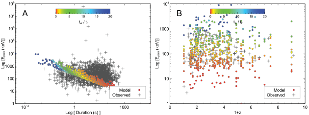
Figure 3: Comparison of our analytical model (§  4.3.2) to LGRB data: Shown are the single thin (i.e. $t_{\rm w}\leq 3t_{\Gamma}$) and thick (i.e. $t_{\rm w}>3t_{\Gamma}$) wall runs compared to observed properties of LGRBs (pluses; from Ghirlanda et al. 2009). The color palette shows the range of the wall thickness parameter $t_{\rm w}/t_{\Gamma}$. There are 500 analytical runs (one per dot) using fiducial parameters given in Table 1. Each run is obtained by varying $t_{\rm QN}$ (i.e. $B_{\rm NS}$) and the viewing angle $\theta_{\rm P}$ with ($0<\theta_{\rm P}<2\times 10^{-3}/N_{\rm c,6}^{1/2}$). The left panel shows the duration compared to the observed $t_{90}$ (data from https://swift.gsfc.nasa.gov/archive/grb_table) while the right panel shows the photon peak energy versus the source redshift. The redshift was obtained by cross-referencing the LGRBs from Ghirlanda et al. (2009) with data in https://swift.gsfc.nasa.gov/archive/grb_table. The redshift $z$ for each run is obtained by randomly selecting a GRB from a global list of 350 GRBs (those with known redshifts) from https://swift.gsfc.nasa.gov/archive/grb_table.

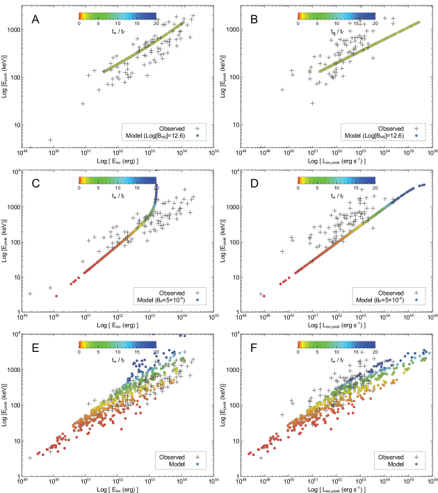
Figure 4: Amati plot (left panels) and Yonetoku plot (right panels) for the single wall analytical model (§  4.3.2): 500 runs (the dots; the pluses are data from Ghirlanda et al. 2009) of the analytical model (including deceleration of chunk for large values of $t_{\rm w}/t_{\Gamma}$). For each run the primary chunk passes through a single wall. Each dot is generated by varying $t_{\rm QN}$ (i.e. $B_{\rm NS}$) and $\theta_{\rm P}$ with ranges similar to those used in Figure 3. Other parameters are set to their fiducial values (see Table 1). The redshift $z$ for each simulation point is obtained by randomly selecting a GRB from a global list of 350 GRBs (those with known redshifts) from https://swift.gsfc.nasa.gov/archive/grb_table. Top panels: Effects of varying the viewing angle $\theta_{\rm P}$ for a fixed $B_{\rm NS}$. Middle panels: Effects of varying $B_{\rm NS}$ for a fixed viewing angle $\theta_{\rm P}$. Bottom panels: Effects of varying both the viewing angle $\theta_{\rm P}$ and the NS magnetic field $B_{\rm NS}$.

We run 500 simulations (the dots in Figures 3 and 4) of our analytical model each representing a single chunk passing through a single thin or thick wall (see Appendix D for key differences between the thin and thick wall cases). The randomized variables are:

• $\theta_{P}=$acos(UniformDistribution[cos($10^{-3}$), 1])

• B${}_{\textrm{NS}}=$ LogNormalDistribution(12.5 log(10), .2 log(10))

• z: Randomly choose a LGRB from a list of over 300 (retrieved from https://swift.gsfc.nasa.gov/archive/grb_table/) and use its z.

For each run, $B_{\rm NS}$ gives us $R_{\rm w}\propto B_{\rm NS}^{-2},n_{\rm w}\propto B_{\rm NS}^{6}$ and $\Delta R_{\rm w}=R_{\rm w}/12$. The other parameters were kept constant to their fiducial values (see Table 1). Our runs are compared to LGRB data (the pluses in Figures 3 and 4). The top left panel in Figure 3 shows $E_{\rm peak}$ ($=E_{\rm\gamma,p}$) versus redshift which is consistent with data. The upper right panel shows $E_{\rm peak}$ versus the GRB duration. The duration is not expected to match the data since the single wall model includes only a single pulse. The slope in the $E_{\rm\gamma,p}$-$\Delta t_{\rm GRB}$ models is due to the fact that $E_{\rm\gamma,p}\propto n_{\rm w}^{1/2}\propto B_{\rm NS}^{3}$ and $\Delta t_{\rm GRB}\propto R_{\rm w}\propto B_{\rm NS}^{-2}$ which yields $E_{\rm\gamma,p}\propto{\Delta t_{\rm GRB}}^{-3/2}$.

We now discuss the Yonetoku and Amati laws resulting from our analytical single wall model. The Yonetoku law is shown in the right panels in Figure 4 while the Amati law is in the left panels. Best overall fits were obtained by adjusting the number of pairs from 10 to $n_{\textrm{pairs}}=20$.

The top panels show the case of a constant $B_{\rm NS}$ and varying viewing angle $\theta_{\rm P}$. The slope in our model agrees better with Amati law than with Yonetoku’s. In the middle panels where the viewing angle is kept constant while varying $B_{\rm NS}$, there is a better agreement with Yonetoku’s but a clear deviation from Amati’s for the high $t_{\rm w}/t_{\Gamma}>10$ sources; we refer to this as the “hook”. Both laws appear to be restored when varying both $B_{\rm NS}$ and the viewing angle as shown in the bottom panels.

In general for the very thick wall case (i.e. $t_{\rm w}/t_{\Gamma}>10$), the Amati relationship is not preserved unless the chunk’s viewing angle $\theta_{\rm P}$ is varied from source to source. However even when varying $\theta_{\rm P}$ between sources there are still some leftover effect of the “hook” in the bottom left panel for the thickest filaments.

4.3.2 The phenomenological Yonetoku and Amati laws

These two-components relationships are in fact phenomenological and are an artifact of limited parameter space (i.e. a limited scatter effect) describing a GRB in our model. For example, $L_{\rm iso,peak}$ ($=L_{\rm GRB}$) for a single chunk is given by Eq. (31) and depends on $\theta_{\rm P},m_{\rm c},\Gamma_{\rm QN}$, and $n_{\rm w}\propto t_{\rm QN}^{3}\propto B_{\rm NS}^{-6}$. Most parameters vary only by a small amount, so we set them to their fiducial values, as we did above, in the following analysis. The two parameters that have significant variation are $\theta_{\rm P}$ and $B_{\rm NS}$.

Expressing $L_{\rm iso}$ ($=L_{\rm GRB}),E_{\rm peak}\ (=E_{\rm\gamma,p})$ and $E_{\rm iso}$ ($=E_{\rm GRB}$) in terms of their dependence on $\theta_{\rm P}$ and $B_{\rm NS}$, we obtain for the thin wall case ($t_{\rm w}^{\prime}/t_{\Gamma}^{\prime}<\sim 3$):

$$E_{\rm peak} =C1\times\frac{n_{\rm w}^{1/2}}{f(\theta_{\rm P})}=C1^{\prime}\times\frac{B_{\rm NS}^{3}}{f(\theta_{\rm P})}$$ (55)

$$L_{\rm iso,peak} =C2\times\frac{n_{\rm w}}{f(\theta_{\rm P})^{4}}=C2^{\prime}\times\frac{B_{\rm NS}^{6}}{f(\theta_{\rm P})^{4}}$$

$$E_{\rm iso} =C3\times\frac{n_{\rm w}R_{\rm w}}{f(\theta_{\rm P})^{3}}=C3^{\prime}\times\frac{B_{\rm NS}^{4}}{f(\theta_{\rm P})^{3}}\ ,$$

with $C1(C1^{\prime}),C2(C2^{\prime})$ and $C3(C3^{\prime})$ constants. The expressions in the middle are for the general case of $t_{\rm QN}\neq t_{\rm SpD}$ while the expressions to the right are for $t_{\rm QN}=t_{\rm SpD}$. Here we focus on the $t_{\rm QN}=t_{\rm SpD}$ case to demonstrate the phenomenological nature of the Yonetoku and Amati laws but this can be easily extended to the general case of $t_{\rm QN}\neq t_{\rm SpD}$.

We see that we cannot write $L_{\rm iso,peak}=f(E_{\rm peak})$ (i.e. as a function of $E_{\rm peak}$ alone) or $E_{\rm iso}=f(E_{\rm peak})$ because they are two independent variables. I.e. $L_{\rm iso,peak}$ is not a function of $E_{\rm peak}$, nor is $E_{\rm iso}$. Thus both Yonetoku and Amati plots will yield a scatter of points about the relation, for which the scatter is determined by the range of $B_{\rm NS}$ and $f(\theta_{\rm P})$.

Let us consider two options:

• If we take $B_{\rm NS}=constant$, then $L_{\rm iso,peak}$ varies as $E_{\rm peak}^{4}$ and $E_{\rm iso}$ varies as $E_{\rm peak}^{3}$. These slopes are recovered in the 500 analytical models shown in the top panels in Figure 4. In the constant $B_{\rm NS}$ case, the thickness parameter is constant (here $t_{\rm w}^{\prime}/t_{\Gamma}^{\prime}=t_{\rm w}/t_{\Gamma}\sim 3$) since the wall’s properties ($n_{\rm w},R_{\rm w}$ and $\Delta R_{\rm w}=R_{\rm w}/12$) are all constant.

• If we take $\theta_{\rm P}=constant$, then $L_{\rm iso,peak}$ varies as $E_{\rm peak}^{2}$ and $E_{\rm iso}$ varies as $E_{\rm peak}^{4/3}$. These slopes are also recovered in the middle panels in Figure 4. Note that the thick wall models (with $t_{\rm w}^{\prime}>3t_{\Gamma}^{\prime}$) deviate slightly from these correlations and are violated for extreme cases when $t_{\rm w}^{\prime}>10t_{\Gamma}^{\prime}$.

• The bottom panels in Figure 4 show the 500 models when both $\theta_{\rm P}$ and $B_{\rm NS}$ are varied. In our analytical model, $\log(B_{\rm NS})$ has a scatter of $\sim 0.2$, and $f(\theta_{\rm P})$ varies between 1 and $\sim 41$. Using $\sigma_{\log{B_{\rm NS}}}\sim 0.5$ gives a much larger vertical and horizontal scatter (i.e. about $\sim 5$ times bigger) in the bottom panels.

In summary, neither the Yonetoku and Amati relations are fundamental, but are phenomenological (as also demonstrated with sumulations in §  5.3.8). According to our model, they are both the result of GRB dependence (i.e. $L_{\rm iso,peak},E_{\rm peak}$ and $E_{\rm iso}$) on multiple physical parameters, which each have a limited range of scatter. Observationally, selection effects (e.g. cut-offs due to detector sensitivity as discussed for example in Collazzi et al. 2012) can result in limited scatter thus yielding in principle phenomenological correlations as described in our model.

To understand the related slopes as reported in the literature we argue the following:

• The slope in the Yonetoku law: Taking different values of $\theta_{\rm P}$ gives a succession of parallel lines each with a slope of 4/3. Taking different values of $B_{\rm NS}$ gives a succession of parallel lines each with a slope of 3. These series of lines in the $L_{\rm iso,peak}$-$E_{\rm peak}$ plane create a scatter which when fit yields a phenomenological slope in the range

  $$\frac{4}{3}\leq{\rm Slope}_{\rm Yonetoku}\leq 3\ .$$ (56)

  The lower limit corresponds to a scatter dominated by a big range in $\theta_{\rm P}$ while the upper limit correspond to a wider range in $B_{\rm NS}$.

• The slope in the Amati law: Taking different values of $\theta_{\rm P}$ gives a succession of parallel lines each with a slope of 2. Taking different values of $B_{\rm NS}$ gives a succession of parallel lines each with a slope of 4. These series of lines in the $E_{\rm iso}$-$E_{\rm peak}$ create a scatter which when fit yields a phenomenological slope of

  $$2\leq{\rm Slope}_{\rm Amati}\leq 4\ .$$ (57)

  The lower limit corresponding to a scatter dominated by a big range in $\theta_{\rm P}$ while the upper limit correspond to a wider range in $B_{\rm NS}$.

We revisit the phenomenological Yonetoku and Amati laws in §  5.3.8.

5 Application to long duration GRBs II: A turbulent filamentary PWN-SN ejecta

The single filament model (i.e. considering only the analytical self-similar wall), while it helps to understand our engine and is successful at capturing key and general features of our model, cannot reproduce the wider variation in duration observed in GRBs, the Band function for the thin wall case and, does not allow for variable luminosity. Here we consider the case of the QN chunks interacting with a turbulent, filamentary, PWN-SN shell in the blow-out regime defined by $P_{\rm NS}<4\ {\rm ms}/{E_{\rm SN,51}}^{1/2}$ (i.e. when $E_{\rm SN}<E_{\rm SpD}$; see Eq. (19)).

The top panel in Table 2 is a summary of the different stages in the blow-out regime. This regime was simulated in Blondin & Chevalier (2017) and consists of a pre-blow-out stage (Figures 3 in that paper) and a blow-out stage (Figure 6 in that paper). These Figures demonstrate how the self-similar solution is modified in 2-Dimensional simulations. Figure 3 in Blondin & Chevalier (2017) shows that in the pre-blow-out stage, roughly 50% of the wall is turbulent and filamentary from the broken off Rayleigh-Taylor (RT) fingers filling the PW bubble interior. The remaining $\sim$ 50% of the wall is in a quasi-spherical self-similar layer between the filaments and the unperturbed density plateau.

In the blow-out stage, the wall and the SN ejecta are torn apart as shown in 2-Dimensional (Figure 6 in Blondin & Chevalier (2017)) and 3-Dimensional simulations (Figures 7 and 9 in Blondin & Chevalier (2017)). The Rayleigh-Taylor fingers split into numerous smaller “filaments” with density varying from much less than the wall’s to that of the wall with most filaments having a density of the order of the plateau’s density. The highly filamentary PWN-SN is extended ($>>R_{\rm w}(t_{\rm Plat,})$) forming large low density corridors. This stage is of particular interest to us since it gave best fits to LGRB data in our model, as we show in section §  5.3.

5.1 The prompt emission

To ensure that the QN occurs when the PWN-SN is in the blown-out stage we set $P=2$ ms instead of $P=4$ ms as adopted earlier in the analytical model. Eq. (19) implies that $t_{\rm Plat.}\sim t_{\rm SpD}/4$ or equivalently that $t_{\rm QN}=t_{\rm SpD}\sim 4t_{\rm Plat.}$ with $t_{\rm SpD}\simeq 25.9$ years for the mean magnetic field value of $B_{\rm NS}=10^{12.5}$ G. Figure 7 in Blondin & Chevalier (2017) shows the PWN-SN shell at $7t_{\rm Plat.}$ which helps us picture the geometry of the blown out turbulent PWN-SN ejecta.

To simulate the filamentary shell in the blow-out regime, we: (i) scale the blow-out PWN-SN ejecta with respect to $R_{\rm w}(t_{\rm Plat.})$ which is the radius of the edge of the SN density plateau when it is reached by the wall; i.e. the start of blow-out when $R_{\rm w}(t_{\rm Plat.})=R_{\rm Plat.}(t_{\rm Plat.})$. For $P_{\rm NS}=2$ ms, we have $t_{\rm Plat.}=t_{\rm SpD}/4\simeq 6.5$ years which gives $R_{\rm Plat.}(t_{\rm Plat.})\sim 10^{16}$ cm (see Eq. (13)); (ii) consider filaments distributed radially with filament radius $R_{\rm F}$ in the range $R_{\rm F,in}\leq R_{\rm F}\leq R_{\rm F,out}$. In general, $10^{-3}R_{\rm w}(t_{\rm Plat.})<R_{\rm F,in}<4R_{\rm w}(t_{\rm Plat.})$ and $R_{\rm w}(t_{\rm Plat.})<R_{\rm F,out}<10^{3}R_{\rm w}(t_{\rm Plat.})$; (iii) set the filaments’ maximum density to $n_{\rm w}(t_{\rm Plat.})$ given by Eq. (17); (iv) include time dependence of $\Gamma_{\rm FS}(t^{\prime})$ since the assumption of $\Gamma_{\rm FS}(t^{\prime})\simeq\Gamma_{\rm QN}$ used in the previous section is no longer valid.

Before we present detailed fits of our model to the light-curves and spectra of observed LGRBs (§  5.3), we briefly described how the prompt emission is modified in the multiple filaments case when compared to the analytical results obtained in the single filament case presented in the previous section. We also demonstrate that a Band-like spectrum is an outcome of the turbulent PWN-SN scenario.

5.1.1 Variability

The spraying of the blown-out PWN-SN ejecta by the millions of QN chunks and their tiny size (compared to the filaments’ radial extent) together with the radial distribution of the filaments yields highly variable LGRBs in our model. Chunks colliding with the very irregular structure of the turbulent PWN-SN ejecta yields very different bursts (i.e. light-curve shapes) for different lines-of-sights. Key points of the picture we present here include:

• The number of filaments the chunks interact with can vary from a few to hundreds;

• For the primary chunk (with $\theta_{\rm c}=\theta_{\rm P}$), the complexity of the turbulent filaments it passes through defines the intrinsic variability and the number of spikes/pulses in the resulting light-curve;

• The brightest spike correspond to when the chunk first hits a high density filament, which can occur anywhere between $R_{\rm F,in}$ and $R_{\rm F,out}$;

• Once the primary hits a thick filament (i.e. when the thickness parameter of filament “F” is $t_{\rm F}^{\prime}/t_{\Gamma}^{\prime}>>1$; here $t_{\rm F}^{\prime}=\Delta R_{\rm F}/\Gamma_{\rm FS}c$), it slows down drastically, effectively putting an end to the prompt emission;

• The observed variability is a convolution between the observer’s time resolution (i.e. binning which we take to be 64 ms in this work) and the filamentary structure of the PWN-SN ejecta. Whenever the radial time delay corresponding to the separation between two filaments ($\Delta R_{\rm F,sep.}^{\rm obs.}$ in the observer’s frame) is less than 64 ms, the resulting spikes will not be resolved. In general, the condition $\Delta t_{\rm F,sep.}^{\rm obs.}=\Delta R_{\rm F,sep.}/D(\Gamma_{\rm FS},\theta_{\rm P})\Gamma_{\rm FS}c>64$ ms translates to a minimum observable filament separation in the NS frame of

  $$\Delta R_{\rm F,sep.}>3.8\times 10^{16}\ {\rm cm}\times\frac{\Gamma_{\rm c,3.5}^{2}}{f(\theta_{\rm P})}\ .$$ (58)

  I.e. to a first order, the observed distinct spikes in GRBs implies a minimum separation between filaments given by Eq. (58).

5.1.2 The duration

The observed duration of emission is due to the radial extent of filaments so that $\Delta t_{\rm GRB}\sim(R_{\rm F,out}-R_{\rm F,in})/D(\Gamma_{\rm FS},\theta_{\rm P})\Gamma_{\rm FS}c$ where $R_{\rm F,in}$ and $R_{\rm F,out}$ are the radii of the innermost and outermost filaments. For the case of $R_{\rm F,out}>>R_{\rm F,in}$ we can write

$$\Delta t_{\rm GRB}\sim\left(\frac{1}{6}\ {\rm s}\times f(\theta_{\rm P})\right)\times\frac{R_{\rm F,out,18}}{\Gamma_{\rm FS,3.5}^{2}}\ .$$ (59)

For $0<\theta_{\rm P}<2/N_{\rm c}^{1/2}$ and for the range of $R_{\rm w}(t_{\rm Plat.})$ given in Eq. (25) we arrive at

$$\frac{1}{600}\ {\rm s}<\Delta t_{\rm GRB}<1.1\times 10^{3}\ {\rm s}\ .$$ (60)

Longer durations than given by Eq. (60) can be obtained when we take into account the slowing down of the chunks from one filament to another (see §  5.3) .

5.2 The Band function

A primary chunk hitting a single wall yields synchrotron emission in the fast cooling regime in our model; see Eq. (42). The corresponding spectrum, given by Eq. (11) in Appendix E, has a photon peak energy at $E_{\gamma,p}$. To explain how a Band function results in our model we consider the scenarios of a single primary chunk: (i) hitting a single non-turbulent thick filament (i.e. a repeat of the single wall model); (ii) going through many thin filaments each at different density $n_{\rm F}$ in a turbulent PWN-SN ejecta.

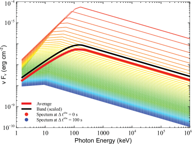
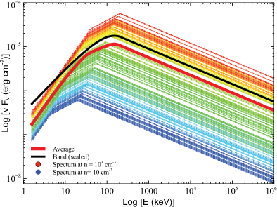
Figure 5: The Band-like spectrum in our model: Top panel: A single chunk going through one high density wall ($n_{\rm w}=10^{5}$ cm^-3, $R_{\rm w}=10^{18}$ cm and $\Delta R_{\rm w}=10^{17}$ cm). Different colors correspond to increasing time. The thick red curve is the time-averaged model spectrum. The thick black curve is a generic Band function. Bottom panel: A single chunk going through multiple thin filaments ($\sim$ 120) with density randomly drawn between $n_{\rm F}=10$ cm^-3 and $n_{\rm F}=1000$ cm^-3. The individual spectra are taken at the beginning of each filament.

The spectrum from the primary chunk hitting a single thick wall is shown in the top panel of Figure 5 (thick red line) which agrees very well with the observed standard Band function (thick black line). Also shown in this panel are spectra sampled within the thick filament starting from the moment the chunk enters the wall until it exits the wall. This demonstrates that the individual spectra add up to the Band one as a result of different Lorentz factors as the chunk slows down.

The bottom panel in Figure 5 shows the spectrum resulting from the same chunk going through many (here 120) thin filaments. In this example, the chunk’s FS Lorentz factor $\Gamma_{\rm FS}$ varies little from filament to filament although the cumulative effect results in decreasing from $\Gamma_{\rm QN}=10^{3.5}$ to about $2800$ at the exit of the last thin filament. A band spectrum is also recovered here.

The Band function is always recovered in our model particularly when varying other parameters (i.e. besides $\Gamma_{\rm FS}$ and $n_{\rm F}$) from one filament to another. The convolving effect of these parameters results in an averaging of the low-energy index in the fast cooling regime yielding the typical low-energy slope in a Band-like spectrum. Effectively, the convolution “smears out” and smooths out the lower limit $E_{\rm\gamma,c}$ (see Eq. (46)) and yield a convolved low-energy slope/index by averaging over the 1/3 and -1/2 slopes of the fast cooling regime (the case in our model; see Eq. (42)). An approximation to the convolved spectrum is given by

$$F(E_{\gamma})\propto\begin{cases}\sim E_{\gamma}^{\frac{1/3-1/2}{2}}=E_{\gamma}^{-\frac{1}{12}},&\text{if }E_{\gamma}<E_{\rm\gamma,p}\\ \sim E_{\gamma}^{-p/2}=E_{\gamma}^{-1.2},&\text{if }E_{\gamma}>E_{\rm\gamma,p}\end{cases}$$ (61)

We thus have $E_{\gamma}^{-1}F(E_{\gamma})\sim E_{\gamma}^{-13/12}$ for the low-energy index and $E_{\gamma}^{-1}F(E_{\gamma})\sim E_{\gamma}^{-2.2}$ (for our fiducial value of $p=2.4$) for the high-energy index. The resulting spectrum is consistent with the Band’s function with an observed low-energy index of $\alpha\sim-1$ and an observed high-energy index of $\beta\sim-2.2$.

Table 2: LGRBs and FRBs in our model (numerical values are for fiducial parameter values (see Table 1))

GRBs: The blow-out regime (i.e. $E_{\rm SN}\leq E_{\rm SpD}$)a
Stageb	Time delay	$B_{\rm NS}$	Burst type	Contribution to GRB rate ($r_{\rm LGRB}$)c
Post-blow-out	$t_{\rm SLSN}<t_{\rm QN}<t_{\rm QN,RS}$	$10^{13}\ {\rm G}<B_{\rm NS}<2.4\times 10^{13}$ G	LGRB $+$ (bright Type Ic-BL SN)d	$<5$%
(Highly-turbulent Wall)
Post-blow-out	$t_{\rm QN,RS}<t_{\rm QN}<t_{\rm SN,RS}$	$1.5\times 10^{12}\ {\rm G}<B_{\rm NS}<10^{13}$ G	LGRB $+$ ($t_{\rm QN}$ old Type Ic SN)e	$>95$%
(Highly-turbulent Wall)
FRBs: The non-blow-out regime (i.e. $E_{\rm SN}>E_{\rm SpD}$)f
Stageg	Time delayh	$B_{\rm NS}$	Burst type	$r_{\rm FRB}/r_{\rm GRB}$
Non-turbulent Wall	$t_{\rm SLSN}<t_{\rm QN}<t_{\rm SN,RS}$	$1.5\times 10^{12}\ {\rm G}<B_{\rm NS}<2.4\times 10^{13}$ G	FRB $+$ UHECRs	See §  6.7
(Onset of Weibel instability)

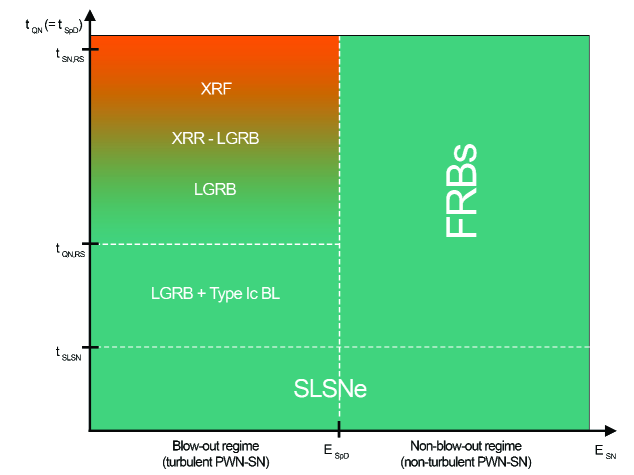
Figure 14: The unification of bursts in our model: The two regimes correspond to the blow-out regime ($E_{\rm SN}<E_{\rm SpD}$) and the non-blow-out regime ($E_{\rm SN}<E_{\rm SpD}$). The non-blow-out regime yields FRBs in our model since the non-turbulent, weakly magnetized, PWN-SN shell is prone to the Weibel instability, triggering coherent synchrotron emission (CSE) in the chunk’s shock (see §  6). The blow-out regime yields LGRBs, XRR-GRBs and XRFs (see §  8.2). For both regimes SLSNe result if the QN occurs on timescales $\leq t_{\rm SLSN}$ when the PWN-SN shell is still optically thick.

^a This case has $t_{\rm SpD}\geq t_{\rm Plat.}$ since $t_{\rm Plat}\sim(E_{\rm SN}/E_{\rm SpD})\times t_{\rm SpD}\sim(E_{\rm SN,51}P_{\rm NS,-2.4}^{2})\times t_{\rm SpD}$; see Eq. (19). For example, $P_{\rm NS}=2$ ms gives $t_{\rm QN}=t_{\rm SpD}\sim 25.9$ yrs and $t_{\rm Plat.}=(1/4)t_{\rm SpD}\sim 6.5$ yrs.
^b The Pre-blow-out stage of the blow-out regime (i.e. $t\leq t_{\rm Plat.}$) is not considered here since $t_{\rm QN}=t_{\rm SpD}>t_{\rm Plat.}$ in our model.
^c We use a lognormal distribution of $B_{\rm NS}$ with mean $10^{12.5}$ G and variance $\sigma_{\log{B_{\rm NS}}}=0.3$ based on our best fits to LGRB data (see §  5.3).
^d Re-brightened by the QN chunks experiencing a reverse shock (RS; see §  5.4.1).
^e The parent type-Ic SN seen at time $t_{\rm QN}=t_{\rm SpD}$.
^f The PWN eventually stalls and the wall becomes “frozen” to the SN ejecta. I.e. $t_{\rm Plat.}$ is meaningless in the non-blow-out regime.
^g The PWN is low-power resulting in a non-turbulent or weakly turbulent PWN-SN shell with weak magnetic field (i.e. $\epsilon_{\rm w}<\epsilon_{\rm w,WI}$, the critical value for the onset of the Weibel instability; see §  6).
^h In both blow-out and non-blow-out regimes, and for $t_{\rm QN}\leq t_{\rm SLSN}\simeq 1.8\ {\rm yrs}$, the wall (i.e. PWN-SN shell) is optically thick yielding a SLSN (see Figure 14).

5.3 Light-Curve and Spectral Fitting

We have fit our model to the light-curves and spectra of 48 observed and well measured LGRBs. In fitting the light-curve, we recall that emission is caused by the interaction of the chunks with the filaments. Therefore, to first order, the position/width of each filament affects the variability in time whereas the density of the filaments affects the variability in flux. The light-curve (the prompt and afterglow emissions) will be dominated by the chunk moving closest to our line of sight at an angle $\theta_{\rm P}$. The flare is due to the secondary chunk at an angle $\theta_{\rm S}$.

5.3.1 Data

Table LABEL:table:lcfits lists the 48 selected LGRBs. These sources were chosen because they all have an abundance of data points and their spectral parameters are available.

The light-curve data for these sources were obtained from the The Swift Burst Analyser (Evans et al. 2010) and consists of a combination of BAT and XRT data over the energy range of 0.3-10 keV (the XRT band). The BAT data has been extrapolated to this XRT band (Evans et al. 2010).

The spectra of many LGRBs can be described by a Band function. We compare our model spectrum to the best fit Band parameters for the sources above, obtained from Yonetoku et al. (2010).

5.3.2 Chunks and Filaments

Our simulations consist of identical chunks distributed isotropically on the sky. The initial Lorentz factor and mass of each chunk are fixed to our fiducial values of $10^{3.5}$ and $10^{22.5}$ gm, respectively (see Table 1).

Each chunk travels through a succession of ‘filaments’. A filament represents a region of space with a certain density $n_{\rm F}$, thickness $\Delta R_{\rm F}$ and magnetic field $B_{\rm F}$. The algorithm for finding the location, thickness and density of each filament is explained in §  5.3.3 below. The magnetic field is determined using Eq. (18) once a filament’s properties are derived.

We only consider chunks within a small angle of the observer (see above) and therefore assume the filaments these chunks encounter are identical. Beyond the filaments is an extended region that represents the ambient medium, with $n_{\textrm{amb.}}$ and $B_{\textrm{amb.}}$. This last region is what governs the afterglow of the GRB and is represented in our simulation as a “wide filament” with density $n_{\rm amb.}$ and magnetic field $B_{\rm amb.}$.

In order to fit the LGRB light-curve, we determine where each filament is located. It is possible to distribute filaments randomly to produce a “generic” light-curve, but this method is not feasible when fitting individual LGRBs (the probability of placing the filaments at the right location is essentially 0). We therefore assume that each observed point represents the interaction of the primary chunk ($\theta_{\rm c}=\theta_{\rm P}$) with a filament. The point with the highest flux corresponds to the filament with a maximum density of $n_{w}$ (Eq. (17)). The density of the filaments corresponding to the remaining points are scaled accordingly, which means no filament has a density greater than $n_{w}$.

5.3.3 Simulation

The simulation generates the light-curve and spectrum, simultaneously for a given set parameters, using the following algorithm:

1. Determine the location, width and density of each filament using the primary chunk (see Appendix E.1).

2. Determine each filament’s density using the peak luminosity (see Appendix E.2).

3. Create the light-curve using the procedure outlined in Appendix E.3.

4. Create the spectrum using the procedure outlined in Appendix E.4.

5.3.4 Fitting

We fit our model to observations by repeatedly generating simulations (5.3.3) with different parameters. The parameters we vary to fit the prompt emission are:

1. $\theta_{\rm P}$: The smallest angle to our line of sight of any chunk in the simulation. This “primary” chunk will have the greatest contribution to the light-curve / spectrum. Decreasing $\theta_{\rm P}$ has the effect of increasing the luminosity of the light-curve and spectrum and shifting the peak of the spectrum to higher energies.

2. $B_{\textrm{NS}}$: The magnetic field of the precursor neutron star (which also sets the time delay since $t_{\rm QN}=t_{\rm SpD}$). This parameter helps determine the density of the filaments and therefore has a strong influence on the overall luminosity. The luminosity of the afterglow is directly effected by $B_{\textrm{NS}}$ because a higher value implies greater filament density, which means the chunk is moving slower when it enters the ambient medium.

3. $n_{\textrm{pairs}}$: The number of electron/positrons created per proton from pair-production. Increasing this parameter shifts the peak of the spectrum to lower energies, while increasing the luminosity of both the light-curve and spectrum.

4. $\epsilon_{\rm w}$: The ratio of magnetic to thermal energy in the turbulent PWN-SN shell. Decreasing $\epsilon_{\rm w}$ serves to shift the peak of the spectrum to higher energies, and steepen the low energy slope of the spectrum.

5. $p$: The power-law index describing the distribution of electron energies. It is used in the synchroton equations (see Eqs. (10) and (11)). This value is fixed by the observed spectrum (in order to match the slope of the high energy tail).

6. $n_{\textrm{amb.}}$: The number density of particles in the final region of our simulation (the ambient medium). This parameter contributes to the slope and luminosity of the afterglow. Increasing $n_{\textrm{amb.}}$ has the effect of steepening the slope of the afterglow decline, and increasing its overall luminosity.

7. $Scale_{\rm P}$: A scaling factor (either by chunk mass or number of chunks, or both) of the primary chunk’s luminosity necessary to fit a few LGRBs when $\theta_{\rm P}=0$. The scaling is an upward shift of the entire light-curve.

Due to the number of parameters (7 that are adjustable), and the time required to generate one simulation, an automatic fitting of the data is not feasible. We therefore manually vary each parameter and rerun the simulation. We determine the “best-fit” simulation by eye.

5.3.5 Results

The results of fitting our model to the 48 sources described in §  5.3.1 are given in Figure 6 with the “best-fit” parameters listed in Table LABEL:table:lcfits.

Table 3: The “best-fit” parameters^a from the QN model for 48 LGRB sources.

#	Source	$\theta_{\rm P}[\textrm{rad}]$	$\log{n_{\textrm{amb.}}}[\textrm{cm}^{-3}]$	$n_{\textrm{pairs}}$	$\log{\epsilon_{\rm w}}$	$p$	$\log{B_{\textrm{NS}}[\textrm{G}]}$	$F_{0}^{\mathbf{b}}$	$F_{1}^{\mathbf{b}}$	$Scale_{\rm P}^{\mathbf{c}}$	$\theta_{\rm S}[\textrm{rad}]^{\mathbf{d}}$	$Scale_{\rm S}^{\mathbf{e}}$
1	050126	1.00E-3	2.00	13.00	-5.70	2.50	12.55	0.44	6.16	1.00	3.00E-3	0.20
2	050315	0.00	0.50	7.00	-5.80	2.08	12.30	3.03E-2	14.72	1.00	5.50E-4	0.50
3	050318	4.20E-4	1.60	26.00	-5.80	2.20	12.50	0.2	9.16	1.00	-1.00	-1.00
4	050319	3.00E-4	1.20	25.00	-5.80	2.70	12.40	0.2	8.08	1.00	1.50E-3	1.00
5	050401	1.00E-4	1.00	26.00	-6.00	3.10	12.36	0.04	18.64	1.00	-1.00	-1.00
6	050505	3.20E-4	1.00	10.00	-6.10	2.50	12.25	1.28E-2	8.12	1.00	-1.00	-1.00
7	050814	0.00	1.50	10.00	-6.30	2.50	12.28	1.28	39.40	1.00	4.00E-4	1.00E-2
8	050820A	2.50E-4	0.00	8.00	-5.80	2.50	12.35	2.40E-2	58.36	1.00	-1.00	-1.00
9	050904	2.00E-4	2.40	4.00	-6.60	2.50	12.30	2.24	85.64	5.00	1.50E-3	1.00
10	050908	4.80E-4	3.00	21.00	-5.80	2.50	12.35	0.08	2.80	1.00	3.00E-3	10.00
11	051109A	1.00E-5	0.50	24.00	-5.80	2.50	12.30	0.16	62.80	1.00	-1.00	-1.00
12	060115	3.50E-4	1.50	16.00	-6.20	2.50	12.45	0.16	31.52	1.00	1.30E-3	0.10
13	060124	3.50E-4	0.20	8.00	-5.80	2.50	12.25	0.12	23.16	1.00	-1.00	-1.00
14	060210	0.00	1.40	8.00	-5.80	2.50	12.32	2.66E-2	51.76	10.00	-1.00	-1.00
15	060223A	5.00E-4	3.00	25.00	-5.70	2.50	12.53	2.86E-2	8.16	1.00	-1.00	-1.00
16	060510B	2.00E-4	1.50	16.00	-5.12	2.50	12.38	3.16	36.76	1.00	7.50E-4	0.80
17	060522	4.00E-4	2.20	11.00	-6.20	2.50	12.78	3.12	80.24	1.00	1.40E-3	0.40
18	060526	1.80E-4	1.60	25.00	-6.10	2.50	12.28	0.04	33.88	1.00	-1.00	-1.00
19	060604	9.00E-4	1.50	15.00	-5.80	2.50	12.38	0.20	6.40	1.00	-1.00	-1.00
20	060707	5.00E-4	1.00	12.00	-6.20	2.50	12.43	0.08	4.20	1.00	3.20E-3	15.00
21	060714	3.00E-4	1.50	44.00	-6.40	2.50	12.34	0.40	40.20	1.00	-1.00	-1.00
22	060814	4.80E-4	2.00	16.00	-5.30	2.50	12.68	7.08E-3	40.08	1.00	3.20E-3	10.00
23	060908	3.50E-4	2.00	24.00	-5.90	2.50	12.45	1.40E-2	20.28	1.00	-1.00	-1.00
24	060927	4.00E-4	2.00	19.00	-6.00	2.50	12.51	1.49E-2	8.28	1.00	-1.00	-1.00
25	061007	0.00	2.00	18.00	-6.30	3.20	12.59	0.04	132.04	1.00	1.00E-3	2.00
26	070508	1.80E-4	2.50	20.00	-6.00	2.50	12.60	1.23E-2	40.20	1.00	1.70E-3	10.00
27	070521	2.00E-4	2.20	5.00	-6.50	2.50	12.30	0.04	111.20	1.00	-1.00	-1.00
28	070714B	2.00E-4	3.00	5.00	-6.40	2.50	12.40	3.08E-2	72.24	1.00	1.00E-3	0.05
29	071003	0.00	2.50	3.00	-6.60	2.50	12.30	1.77E-2	269.88	10.00	2.00E-3	2.00E3
30	071010B	7.00E-4	1.00	35.00	-5.00	2.50	12.68	2.63E-2	8.88	1.00	-1.00	-1.00
31	080319Bf,g	0.00	-0.40	10.00	-6.40	5.80	12.62	0.16	298.32	10.00	3.30E-3	10.00
32	080411	0.00	0.00	22.00	-4.72	2.50	12.50	9.20E-3	200.32	1.00	-1.00	-1.00
33	080603B	4.00E-4	2.50	33.00	-5.80	2.50	12.50	0.12	6.16	1.00	1.20E-3	5.00
34	080605	0.00	2.20	6.00	-6.40	2.50	12.26	2.10E-2	258.48	8.00	-1.00	-1.00
35	080607	0.00	2.50	8.00	-6.20	2.50	12.40	2.92E-3	40.20	10.00	-1.00	-1.00
36	080721	0.00	2.20	4.00	-6.80	2.85	12.35	1.56E-2	380.48	50.00	-1.00	-1.00
37	080810	0.00	1.70	8.00	-6.30	2.50	12.40	0.08	29.00	1.00	-1.00	-1.00
38	080916A	6.50E-4	1.80	10.00	-6.30	2.50	12.50	2.56E-2	20.12	1.00	3.00E-3	0.30
39	081121	0.00	1.80	8.00	-6.60	3.01	12.28	0.16	127.88	10.00	-1.00	-1.00
40	090102	0.00	2.50	4.00	-6.60	2.50	12.32	0.04	195.84	20.00	-1.00	-1.00
41	090423	0.00	2.50	6.00	-6.60	2.50	12.28	0.08	134.84	10.00	-1.00	-1.00
42	090424	3.00E-4	0.00	30.00	-6.20	3.80	12.45	5.08E-3	60.20	1.00	1.80E-3	10.00
43	090618g	0.00	1.50	17.00	-5.80	2.99	12.50	3.64E-2	265.28	1.00	5.20E-4	1.00
44	090715B	0.00	2.00	12.00	-6.40	2.50	12.35	0.04	137.28	10.00	-1.00	-1.00
45	090812	3.50E-4	2.00	11.00	-6.40	3.00	12.58	1.06E-2	20.32	1.00	2.30E-3	10.00
46	090926B	3.00E-4	1.80	7.00	-6.60	2.50	12.26	2.29E-2	260.20	1.00	-1.00	-1.00
47	091029	4.00E-4	2.00	15.00	-5.40	2.50	12.51	1.62E-2	20.24	1.00	2.50E-3	30.00
48	091208B	5.50E-4	1.60	26.00	-5.10	2.65	12.44	0.04	40.16	1.00	-1.00	-1.00
a The chunk’s opacity was adjusted to 0.05 cm2 gm-1 for best fits. Other parameters are set to their fiducial values (see Table 1).
b See Appendix E.1 for filament location and thickness generation:
$F_{0}$ = location of the first filament (i.e. $R_{\rm F,in}/R_{\rm w}(t_{\rm Plat.})$). $F_{1}$ = location of the last filament (i.e. $R_{\rm F,out}/R_{\rm w}(t_{\rm Plat.})$).
Blow-out occurs at $t_{\rm Plat.}$ (see Eq. (19)) when the wall reaches the edge of the density plateau; i.e. $R_{\rm w}(t_{\rm Plat.})=R_{\rm Plat.}(t_{\rm Plat.})$.
c $Scale_{\rm P}$ = scale of the primary chunk’s luminosity.
d $\theta_{\rm S}$ = angle of the secondary fragment (-1 means no secondary needed to fit LGRB; i.e. no flare in the light-curve).
e $Scale_{\rm S}$ = scale of the secondary chunk’s luminosity.
f This source required an extreme value for the electron power-law index, $p=5.8$.
g LGRBs with associated broad-line Type Ic SN; see https://www.dark-cosmology.dk/GRBSN/GRB-SN_Table.html.

5.3.6 Flares

Many LGRBs exhibit X-ray flares which are an increase in brightness by up to a factor of 1000 times from the baseline. In our model, X-ray flares are produced by secondary chunks. The light-curve of a chunk with a $\theta_{\rm S}>\theta_{\rm P}$ will appear shifted to longer times and lower flux. Because this chunk goes through more or less the same filaments as the primary chunk, to a first order the X-ray flare will appear as a “mirror” of the primary prompt emission with the spectrum shifted to lower energies. The parameters we vary to fit the flares are:

1. $\theta_{\rm S}$: The secondary’s angle to our line of sight with $\theta_{\rm S}=\theta_{\rm sep.}-\theta_{\rm P}=4/N_{\rm c}^{1/2}-\theta_{\rm P}$. Decreasing $\theta_{\rm S}$ has the effect of increasing the luminosity of the flare and decreasing the time between the prompt emission and flaring (see §  4.2.6).

2. $Scale_{\rm S}$: A scaling factor (either by chunk mass or number of chunks, or both) of the secondary chunk’s luminosity is needed in order to fit flares in some LGRBs. The scaling consists of a shift of the luminosity of the entire flaring episode.

In Figure 7 (top panel) we have created a generic LGRB to show how chunks with increasing $\theta_{\rm c}$ contribute to the flares. The “LGRB” consists of a single filament and four chunks at $\theta_{\rm c}=0,0.001,0.002,$ and $0.003$ rads. The effect of increasing the $\theta_{\rm c}$ of the chunks is clear; the “spike” in emission occurs later in time and at a lower flux. If the chunks are smoothly distributed in $\theta_{\rm c}$ one would expect a smooth slope as each chunk appears to hit the filament one after another. However, if there is a large gap between $\theta_{\rm P}$ and the next lowest $\theta_{\rm c}=\theta_{\rm S}$ we would expect a large spike in emission (from the $\theta_{\rm P}$ chunk), and then another spike (from the $\theta_{\rm S}$ chunk).

In Figure 7 (bottom panel) we show how this would look with a real LGRB, by using our fit to GRB 060707. The observed data is represented by the black, open circles. A flare is evident around $t^{\textrm{obs}}=10^{2.5}$ s. We show, in purple, the light-curve produced by the primary chunk with $\theta_{\rm P}=4\times 10^{-4}$ rad. The green represents the light-curve produced by a secondary chunk with $\theta_{\rm S}=2.7\times 10^{-3}$ rad. From this figure, it is clear that a “mirror” light-curve is produced by the $\theta_{\rm S}$ chunks, appearing lower in flux and at a later time. Here an upward scaling factor $Scale_{\rm S}=40$ was used. To justify this factor and in general to fit LGRB light-curves with extreme flares (see Table LABEL:table:lcfits), the uniform filament density and uniform Lorentz factor assumptions had to be relaxed. For example, if the secondary chunk collides with a denser part of the filament than the primary does, then the density ratio must be included in Eq. (49) allowing for brighter flares (see discussion in §  5.3.7).

5.3.7 Discussion of our fits to LGRB light-curves

Figure 8 shows the distributions of parameters resulting from our fits to the 48 selected LGRBs. For a fixed NS period of $P_{\rm NS}=2$ ms, the distribution of $B_{\rm NS}$ shown in panel A corresponds to $\sigma_{\log{B_{\rm NS}}}\sim 0.2$ which is narrower than the $\sigma_{\log{B_{\rm NS}}}\sim 0.5$ suggested by analysis of $B_{\rm NS}$ distribution of observed pulsars (e.g. Faucher-Giguère & Kaspi 2006). However, a variation in $P_{\rm NS}$ could widen the distribution. The distribution in the magnetization parameter $\epsilon_{\rm w}$ (panel B) resulting from the fits is consistent with our model’s fiducial values which corresponds to a PWN-SN magnetic field in the milli-Gauss values.

The distribution of the primary chunk’s viewing angle (panel C) has a mean of $\bar{\theta}_{\rm P}\sim 2\times 10^{-4}$ which is less than the analytical (i.e. model) value of $\bar{\theta}_{\rm P}\sim 1.3\times 10^{-3}N_{\rm c,6}^{-1/2}$. This is expected since the 48 selected sources are brighter than average. When $\theta_{\rm P}<<1/\Gamma_{\rm FS}$, the light-curve and spectrum are insensitive to $\theta_{\rm P}$; i.e. we cannot distinguish between $\theta_{\rm P}=0$ and $\theta_{\rm P}\sim 10^{-4}$. This explains the peak in the lowest bin in panel C. Similarly, the distribution of the secondary chunk’s viewing angle (panel D) shows a mean of $\bar{\theta}_{\rm S}\sim 1.3\times 10^{-2}\sim 10\bar{\theta}_{\rm P}$ which exceeds the analytical (i.e. model) value of $\bar{\theta}_{\rm S}\sim 3.1\times 10^{-3}N_{\rm c,6}^{-1/2}\sim 2.4\bar{\theta}_{\rm P}$.

Panel E shows the distribution of the scaling factor $Scale_{\rm P}$ (which allows us to adjust upwards the entire prompt emission to fit data) which is needed in a few (11 of 48) LGRBs. Scaling is also needed to fit flares (see panel F) because of the larger values of $\theta_{\rm S}$ obtained from fits (mainly constrained by the location in time of flares in the LGRB light-curves). There are 8 LGRBs with $Scale_{\rm S}<1$, 10 LGRBs with $Scale_{\rm S}>1$, 1 LGRB with $Scale_{\rm S}=1$ and 27 LGRBs with no flare ($Scale_{\rm S}=-1$; see Table LABEL:table:lcfits). Because we assume that each filament has a uniform density, together with uniform chunk mass and Lorentz factor, flares are in general less bright than the prompt emission. On average $L_{\rm Flare}/L_{\rm GRB}\sim 10^{-3}$ (see §  4.2.6). Large density variations within and between filaments are required to explain extreme flares which is not seen in simulations of the turbulent PWN-SN shell. We find that changing $\Gamma_{\rm c}$ between the primary and secondary chunks to account for large flares would add an extra delay (radial) time to Eqs. (50) and (52) making the fits much more complex. In summary, the physical origin of $Scale_{\rm P}$ and $Scale_{\rm S}$ can be partly due to chunk mass and/or filament density variations.

Panel G shows the distribution of filaments’ density while panel H shows an almost flat distribution in the number of filaments which can vary from a few filaments to hundreds of filaments from one LGRB to another. The location of the innermost filament (panel I) and the outermost filament (panel J) in terms of $R_{\rm w}$ varies widely from one LGRB to another which speaks to the highly filamentary nature of the PWN-SN in the blow-out stage. The distribution of the ambient medium surrounding the SN (panel K) is slightly higher compared to typical ISM density but not unreasonable for the ambient medium immediately after the SN ejecta. Finally, in panel L we show the resulting $n_{\rm pairs}$ distribution with a peak at 10 consistent with our fiducial value (see Table 1). Note that $n_{\rm pairs}$ for a given LGRB does not exceed the limiting value given in Eq. (45) which ensures that synchrotron emission occurs in the fast cooling regime.

Panel A in Figure 9 shows the distribution of $t_{\rm QN}=t_{\rm SpD}$ (the time delay between the SN and QN) for our best fits to light-curves and spectra. It is close to uniform, varying from 10 years to $<100$ years with a peak at $\sim 35$ years consistent with our fiducial value. Since $t_{\rm QN}\propto B_{\rm NS}^{-2}$, the shorter $t_{\rm QN}$ values correspond to higher $B_{\rm NS}$ values (see panel A in Figure 8).

Panel B in Figure 9 shows the distributions of the thickness parameter (i.e. $t_{\rm w}/t_{\Gamma}$) resulting from our fits to the selected LGRBs. This shows that best fits require a range of filament thickness for each LGRB varying from extremely thin walls to very thick walls. As shown earlier, including thick filaments is essential for obtaining a Band function and allows us to simultaneously fit the prompt emission and the afterglow emission. I.e. the drop in luminosity during the transition from prompt to afterglow emission cannot be explained as a density effect alone (recall that $L_{\rm GRB}\propto n_{\rm w}$ while $L_{\rm AG}\propto n_{\rm amb.}$). A simultaneous fit of the prompt and afterglow emission (both scaling as $\Gamma_{\rm c}^{6}$) require slowdown of the primary chunk which can only occur with the presence of a thick filament along the primary’s path.

Finally, the lower panel in Figure 9 shows the distribution of the duration ($t_{90}$) of all observed GRBs. Also shown is the $t_{90}$ of the 48 LGRBs we selected. Our selected LGRBs are representative of the bulk in $t_{90}$ but not in luminosity and photon peak energy which is on average higher than the bulk. The duration of a typical LGRB in our model is evidence for the large the radial extent of the blown out PWN-SN shell when it is hit by the QN chunks. The fits suggest $10^{-1}<R_{\rm F,out}/R_{\rm w}<10^{3}$ as typical for LGRBs.

5.3.8 Revisiting the phenomenological Yonetoku and Amati laws

We start by simulating a single filament case for $P_{\rm NS}=4$ ms ($t_{\rm Plat.}\sim t_{\rm SpD}$) in order to compare it to the analytical single wall case presented in §  4. The filament is at a radius $R_{\rm F}=R_{\rm w}(t_{\rm SpD})$ and has a thickness $\Delta R_{\rm F}=R_{\rm w}(t_{\rm SpD})/12$. Instead of using Eqs. (31), (33), (35) and (47), here the peak of the spectrum (E${}_{\textrm{peak}}$) is obtained from the generated spectrum (see Appendix E.4). Similarly, L${}_{\textrm{iso},\textrm{peak}}$ is read from the generated light-curve (based on a random number of filaments) and the E${}_{\textrm{iso}}$ value is obtained by integrating the light-curve (see Appendix E.3). We use a 64 ms resolution which means that the peak luminosity is the 64-ms-peak-luminosity (see Appendix E for more details).

We run 500 simulations each representing a single chunk passing through a single filament. The main parameters (see Table 1) were kept constant to their fiducial values for each simulation while we randomize:

• $\theta_{\rm P}=$acos(UniformDistribution[cos($10^{-3}$), 1])

• $B_{\textrm{NS}}=$ LogNormalDistribution(12.5 log(10), .2 log(10))

• z: Randomly choose a LGRB from a list of over 300 (retrieved from https://swift.gsfc.nasa.gov/archive/grb_table/) and use its z.

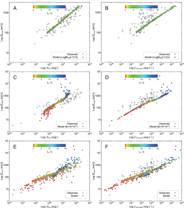
Figure 10: Amati plot (left panels) and Yonetoku plot (right panels) for the single wall numerical simulations model (§  5.3.8): 500 simulations (including deceleration of chunk for large values of $t_{\rm w}/t_{\Gamma}$) are plotted against the observations. For each simulation the primary chunk passes through a single wall. Here all parameters are kept to their fiducial values (see Table 1) except for the number of pairs which is $n_{\rm pairs}=15$ for best agreement with data in the left panels. The dots correspond to 500 simulations but for varied $t_{\rm QN}$ (i.e. $B_{\rm NS}$) and $\theta_{\rm P}$ with ranges similar to those used in Figure 4. Also, binning into 64 ms time bins introduces scatter not present in the analytical case (see Figure 4). Top panels: Effects of varying the viewing angle $\theta_{\rm P}$ for a fixed $B_{\rm NS}$. Middle panels: Effects of varying $B_{\rm NS}$ for a fixed viewing angle $\theta_{\rm P}$. Bottom panels: Effects of varying both the viewing angle $\theta_{\rm P}$ and the NS magnetic field $B_{\rm NS}$.

The resulting points are plotted against the observations (LGRB data is from Ghirlanda et al. 2009) in Figure 10 . The simulation results are close to the analytical models shown in Figure 4. The binning into 64 ms time bins introduces scatter in Figure 10 which is not present in Figure 4.

As shown in Figure 10, the Amati law (panels A, C and E) is preserved up to a few times $t_{\rm w}/t_{\Gamma}$. In particular by adjusting the number of pairs to $n_{\textrm{pairs}}=15$ we obtain overall better fits to the Amati data although this results in the model’s points to fall slightly below the data in panels B, D and F (i.e. the Yonetoku law).

The Amati law is not satisfied for the very thick wall case and a “hook”, already seen in panel C in Figure 4, appears in panel C (for $E_{\rm peak}>10^{3}$ keV) in Figure 10. The “hook” is smeared out when $\theta_{\rm P}$ is varied (see panels A and E). If we take $\sigma_{\log{B_{\rm NS}}}\sim 0.5$ instead of $\sigma_{\log{B_{\rm NS}}}\sim 0.2$, the vertical and horizontal scatter is much larger in all panels and erases the “hook”.

When $B_{\rm NS}$ is low, the main LGRB prompt emission and the afterglow become similar in brightness so that the afterglow contributes to $E_{\rm iso}$. In addition, low $B_{\rm NS}$ corresponds to low $E_{\rm peak}$. The corresponding LGRBs are the scattered red dots at lowest $E_{\rm peak}$ values in panel C in Figure 10.

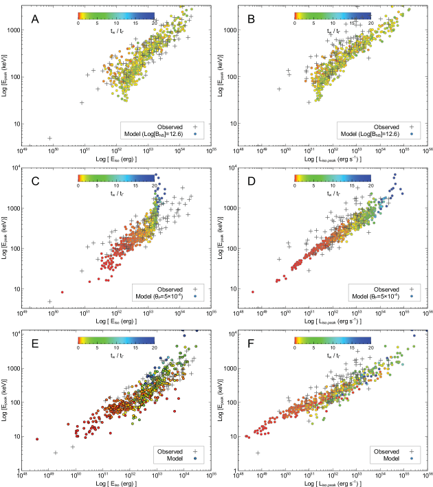
Figure 11: Amati plot (left panels) and Yonetoku plot (right panels) for the multiple filaments numerical simulations model (§  5.3.8): For each simulation a single chunk passes through multiple filaments of varied thickness. The palette shows the highest thickness parameter (i.e. the thickest filament for each case). The dots correspond to 500 simulations but for varied $t_{\rm QN}$ (i.e. $B_{\rm NS}$) and $\theta_{\rm P}$ with ranges similar to those used in Figure 10. Other parameters kept to their fiducial values (see Table 1) except for the number of pairs which is $n_{\rm pairs}=12$ for best agreement with data in the left panels. Top panels: Effects of varying the viewing angle $\theta_{\rm P}$ for a fixed $B_{\rm NS}$. Middle panels: Effects of varying $B_{\rm NS}$ for a fixed viewing angle $\theta_{\rm P}$. Bottom panels: Effects of varying both the viewing angle $\theta_{\rm P}$ and the NS magnetic field $B_{\rm NS}$.

In Figure 11, we redo the analysis considering multiple filaments. Again, we run 500 simulations but now for each simulation there are multiple filaments with radius ranging between $R_{\rm F,in}$ and $R_{\rm F,out}$. The parameters in Table 1 are kept constant to their fiducial values for each simulation except the number of pairs was adjusted to $n_{\textrm{pairs}}=12$ which gave best agreement with data in the left panels representing the Amati law. The randomized variables are:

• $\theta_{\rm P}=$acos(UniformDistribution[cos($10^{-3}$), 1])

• B${}_{\textrm{NS}}=$ LogNormalDistribution(12.5 log(10), .2 log(10))

• $\Delta R_{\textrm{F}}=$ UniformDistribution[0, $\Delta R_{\textrm{w}}=R_{\rm w}/12$]

• $n_{\textrm{F}}=$ UniformDistribution[0, $n_{\textrm{wall}}$]

• z: Randomly choose a LGRB from a list of over 300 (retrieved from https://swift.gsfc.nasa.gov/archive/grb_table/) and use its z.

We take $R_{\rm F,in}=0.2R_{\rm w}$ and $R_{\rm F,out}=2.0R_{\rm w}$ with $R_{\rm w}=R_{\rm w}(t_{\rm SpD})$. Filament generation consists of stacking slabs of density $n_{\rm F}$, including $n_{\rm F}=0$ (i.e. no filament), until $2.0R_{\textrm{w}}$ is reached. The random generation of the filament’s thickness $\Delta R_{\textrm{F}}$ results in a random number of filaments between $0.2$-$2.0R_{\textrm{w}}$ for each simulation run.

In the multiple filament scenario, the phenomenological Yonetoku relationship is preserved since inherently each filament obeys it regardless of the thickness. We arrive at similar conclusions for the Amati law for small and intermediate filament thickness (i.e. $1<t_{\rm w}/t_{\rm\Gamma,w}<10$). As expected for much thicker filaments, the Amati relationship is lost. As in the single filament case, for small values of $\theta_{\rm P}$, the “hook” in $E_{\rm iso}$ in panel C (for $E_{\rm peak}>10^{3}$ keV) in Figure 11 shifts to higher values of $E_{\rm iso}$. This effect can be seen in panels A and E where $\theta_{\rm P}$ is varied.

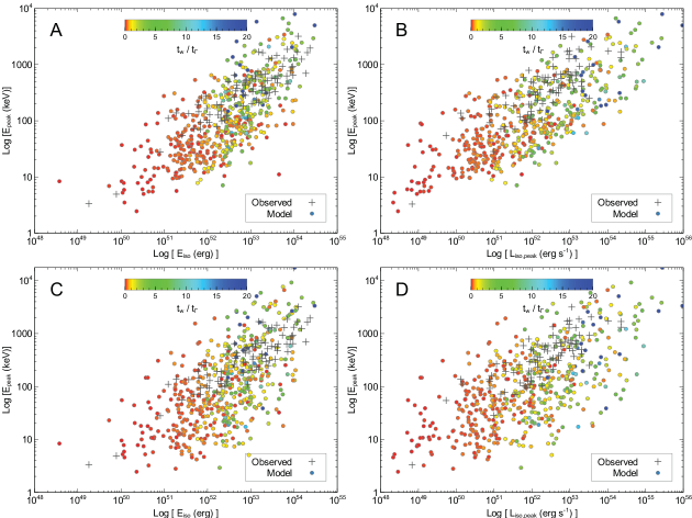
Figure 12: Amati plot (left panels) and Yonetoku plot (right panels) for the multiple filaments case including scatter from other parameters: These are the same simulations as in Figure 11 but this time we include scatter from $n_{\rm pairs}$, $\epsilon_{\rm w}$ and $p$ in the range of Table LABEL:table:lcfits. The two top panels correspond to $5\leq n_{\rm pairs}\leq 30$, while in the two bottom panels we vary simultaneously the three parameters ($5\leq n_{\rm pairs}\leq 30$, $-6.0\leq\log{\epsilon_{\rm w}}\leq-4.5$ and $2<p\leq 3$).

Figure 12 shows the multiple filaments simulations again but this time including a variation in $n_{\rm pairs},\epsilon_{\rm w}$ and $p$ in the range representative of those in Table LABEL:table:lcfits; i.e. $5\leq n_{\rm pairs}\leq 35$, $-6\leq\log{\epsilon_{\rm w}}\leq-4.5$ and $2<p\leq 3$. We see that the trend seen in previous simulations with a limited parameter ranges starts to vanish. In fact using $\sigma_{\log{B_{\rm NS}}}=0.5$ instead of $\sigma_{\log{B_{\rm NS}}}=0.2$ obtained from best fits to the selected LGRBs, gives a significantly larger scatter in the 500 simulations than shown in Figure 11 and Figure 12. Using only bright LGRBs with high photon peak energy (thus eliminating high-$z$ and faint LGRBs), the phenomenological Yonetoku and Amati laws re-appear in our model. Observations would select bright and high $E_{\rm peak}$ LGRBs likely throwing out high-$z$ and faint ones thus reproducing the phenomenological laws.

5.4 Discussion and predictions

5.4.1 The SN/GRB connection

As discussed in §  1.1.2, all SNe associated with LGRBs are classified as broad-line Type Ic with photospheric velocities exceeding $\sim 10,000$-$20,000$ km s^-1 (e.g. Modjaz et al. 2016). These are reminiscent of hypernovae with kinetic energy of order $10^{52}$ ergs (Iwamoto et al. 1998). It is also important to note that not all Type Ic-BL SNe are accompanied by a LGRB which may be attributed to viewing effect (a review of GRB-SNe can be found in Hjorth & Bloom (2012)). These seem to explode with less energy, showing a lower luminosity and mass ejected when compared to those associated with LGRBs (e.g. Nomoto et al. 2006).

In our model, a Type Ic-BL SN can occur simultaneously with a LGRB in the blow-out stage if the filamentary PWN-SN shell is on average dense enough (i.e. there are enough filaments with $n_{\rm F}>n_{\rm w,RS}\sim 2.2\times 10^{7}$ cm^-3; see Eq. (27)) for the RS shock into the chunk to take place. The RS will convert the kinetic energy of the chunks hitting dense filaments to internal energy in a chunk’s crossing time $A_{\rm c,T}^{1/2}/c$ (e.g. Sari & Piran 1995) which is a fraction of a second. The result is an optically thick chunk fireball (with a very large $(e^{+},e^{-})$ density) expanding at $\sim c/\sqrt{3}$ inside the optically thin wall. This late time (i.e. at time $t_{\rm QN}$ after the SN), instantaneous, energy injection as thermal energy into the PWN-SN shell should yield a luminous SN (Leahy & Ouyed 2008; Ouyed, R. et al. 2012) with properties reminiscent of a Type Ic-BL SN.

We offer the following scenario for SN-LGRBs which will be explored elsewhere:

1. A “normal” SN Ic has formed from the collapse of a massive star stripped of its hydrogen and helium (e.g. Filippenko 1997; Heger et al. 2003);

2. It is followed by the SN interaction with a pulsar wind with $E_{\rm SpD}>E_{\rm SN}$ creating a turbulent PWN-SN shell;

3. A QN follows the SN after time $t_{\rm Plat.}<t_{\rm QN}=t_{\rm SpD}<t_{\rm QN,RS}$ when the PWN-SN shell is already blown-out by the PWN. Setting $t_{\rm QN}=t_{\rm SpD}\leq t_{\rm QN,RS}$ with $t_{\rm QN,RS}$ given by Eq. (28) means $B_{\rm NS}\geq 10^{13}$ G when $P=2$ ms. In other words, LGRBs associated with Type Ic-BL SNe occur when $10^{13}\ {\rm G}\leq B_{\rm NS}<2.4\times 10^{13}$ G (see Table 2) with the upper $B_{\rm NS}$ value corresponding to $t_{\rm QN}=t_{\rm SLSN}$ above which the SN ejecta is optically thick (see Eq. (54));

4. The QN chunks interacting with the densest filaments (i.e. those with $n_{\rm F}>n_{\rm w,RS}$) shed their kinetic energy via the RS. Even if we assume that only $\zeta_{\rm QN}=10$% of the chunks’ kinetic energy is converted by the RS into accelerating the entire SN ejecta, this gives an ejecta’s velocity of $v_{\rm SN}\sim 1.4\times 10^{4}\ {\rm km\ s}^{\-1}\times\left(\zeta_{\rm QN,-1}E_{\rm QN,53}M_{\rm SN,34}^{-1}\right)^{1/2}$;

5. Seeing a LGRB along the observer’s line-of-sight (i.e. a primary chunk colliding with a filament with $n_{\rm F}<n_{\rm w,RS}$) means the chunk’s Lorentz factor would have decreased before reaching the subsequent filaments. For example, a decrease of the LGRB Lorentz factor from $10^{3.5}$ to $10^{3}$ would increase the critical density for the RS trigger by a factor of 10 (i.e. $n_{\rm w,RS}=2.2\times 10^{8}$ cm^-3; see Eq. (27)). This means that the LGRB-generating chunk will less likely be subject to the RS but will instead yield an afterglow;

6. On the other hand, a Type Ic-BL SN with no LGRB association would result if the filaments along the observer’s line-of-sight have $n_{\rm F}>n_{\rm F,RS}$;

7. For a range $10^{13}\ {\rm G}\leq B_{\rm NS}<2.4\times 10^{13}$ G and using the lognormal distribution in $B_{\rm NS}$ peaking at $10^{12.5}$ G with variance $\sigma_{\log{B_{\rm NS}}}=0.3$ gives only a few percent of all LGRBs predicted to be associated with Type Ic-BL SNe (see Table 2 and §  5.4.4).

5.4.2 “SN-less” LGRBs

Some LGRBs, in particular those found in metal-rich environments with little star formation (e.g. Tanga et al. 2018), show no underlying Type Ic-BL SNe. In our model, every LGRB is associated with a “faded” SN; i.e. the original type-Ic SN which is to be differentiated from the Type Ic-BL SN occurring at $t_{\rm QN}$ after the SN (see Table 2). However, the time delay of years to decades between the SN and the QN means that the underlying Type Ic SN is too faint to detect. We predict that eventually extremely faint type-Ic SNe will be associated with nearby LGRBs. In our model the formation of an LGRB should be independent of metallicity. As long as a SN leaves behind a NS powerful enough to blow-out the SN ejecta and massive enough to undergo a QN event, a LGRB should result.

5.4.3 “Smooth” LGRBs

For $E_{\rm SN}\sim E_{\rm SpD}$, or equivalently when $P_{\rm NS}\sim P_{\rm NS,cr.}$ (see Eqs. (19) and (20)), then $t_{\rm QN}=t_{\rm SpD}\sim t_{\rm Plat.}$, as in the $P=4$ ms and $E_{\rm SN}\sim 10^{51}$ erg case presented in §  4. This means that the QN occurs at the interface between the pre-blow-out and blow-out stages in the blow-out regime (see Table 2). In this case, $R_{\rm F,out}\sim R_{\rm w}(t_{\rm Plat.})$ and the PWN-SN is less turbulent than in the fully blow-out stage. These LGRBs should yield relatively smoother light-curves according to our model with a wide variation in duration with overlap with SGRB duration (i.e. $<0.1$ s) as clearly shown in panel A in Figure 3 . These short duration LGRBs are more likely be associated with a Type Ic-BL SN since the PWN-SN ejecta is relatively dense as discussed in §  5.4.1. These should be easily distinguishable from SN-less SGRBs which are associated with mergers (see §  7.4). We speculate that SGRB 051221A and SGRB 070724A may be two candidates of short duration LGRBs as discussed here since their duration and hardness hint at a massive star origin (see Bromberg et al. 2013).

5.4.4 LGRB rate in our model

The range in NS magnetic field applicable to LGRBs in our model is given in Eq. (54). Furthermore, our best fits to light-curves is consistent with a lognormal distribution with standard deviation of $\sigma_{\log{B_{\rm NS}}}\sim 0.2$. Making use of the normal distribution of birth periods of NSs with mean of $\mu_{\rm P_{\rm NS}}=300$ ms and standard deviation of $\sigma_{\rm P_{\rm NS}}=150$ ms (e.g. Faucher-Giguère & Kaspi 2006), we can estimate the rate of LGRBs as

$$r_{\rm LGRB} =\frac{\int_{12.2}^{13.4}e^{-\frac{(\log{B_{\rm NS}}-\mu_{\log{B_{\rm NS}}})^{2}}{2\sigma_{\log{B_{\rm NS}}}^{2}}}d\log B_{\rm NS}}{\int_{11}^{15}e^{-\frac{(\log{B_{\rm NS}}-\mu_{\log{B_{\rm NS}}})^{2}}{2\sigma_{\log{B_{\rm NS}}}^{2}}}d\log B_{\rm NS}}\times$$ (62)

$$\times\frac{\int_{1.5}^{4}e^{-\frac{(P_{\rm NS}-\mu_{\rm P_{\rm NS}})^{2}}{2\sigma_{\rm P_{\rm NS}}^{2}}}dP_{\rm NS}}{\int_{1.5}^{\infty}e^{-\frac{(P_{\rm NS}-\mu_{\rm P_{\rm NS}})^{2}}{2\sigma_{\rm P_{\rm NS}}^{2}}}dP_{\rm NS}}\times r_{\rm CCSNE}\times r_{\rm M_{\rm NS,c.}}\ ,$$

where $r_{\rm CCSNE}\sim 1/100$ per year per galaxy is the core-collapse SN rate (e.g. Cappellaro et al. 2015) and $r_{\rm M_{\rm NS,cr.}}$ the percentage of CCSNE giving birth to NSs with mass exceeding $M_{\rm NS,c.}$. The lower value of 1.5 ms in the period distribution takes into consideration the constraints of r-mode instability on rapidly rotating accreting NSs (Andersson et al. 1999, 2000).

We get $r_{\rm LGRB}\sim 0.5\times 10^{-2}\times 10^{-2}\times 10^{-2}\sim 5\times 10^{-7}$ yr^-1 galaxy^-1 (or close to one LGRB per million years per Galaxy) if roughly 1 in 100 CCSNE yield NSs massive enough to explode as QNe. Of these, less than $\sim 5$% yield SN-LGRBs (i.e. LGRB associated with Type Ic-BL SNe; see §  5.4.1 and Table 2 for the corresponding $B_{\rm NS}$ range).

5.4.5 The Blackbody component

In the early stages of the chunk’s evolution, before colliding with the wall, the primary chunk is thermalized up to the transparency radius given by Eq. (13). The time evolution of the properties of this BB precursor is given in Eq. (26). The maximum observed BB photon peak energy, when $\theta_{\rm P}=0$, is $E_{\rm BB,max.}=2\Gamma_{\rm QN}\times(3k_{\rm B}T_{\rm c,T}^{\prime})$. Or,

$$E_{\rm BB,max.}\simeq 4.3\ {\rm keV}\times\Gamma_{\rm QN,3.5}m_{\rm c,22.5}^{-0.194}\kappa_{\rm c,-1}^{-3.3/6.7}\ .$$ (64)

For $t^{\prime}<t_{\rm T}^{\prime}$, the chunks would hit the wall before they become optically thin; particularly in the turbulent PWN-SN scenario where inner filaments form well within the PWN-SN wall. This suggest that the early light-curves of LGRBs should show spikes with a hybrid spectrum which would consist of a BB component (from the chunk proper) and Synchrotron emission (from the FS).

5.4.6 Predictions

• Super LGRB: Because it is due to a single chunk (the primary), the observed prompt LGRB luminosity in our model can be extreme even for an isotropic engine. Eq. (32) gives a maximum value of

  $$L_{\rm GRB,max.}\sim 3.7\times 10^{58}\ {\rm erg\ s}^{-1}\ .$$ (65)

  Eq. (65) also implies that the observed isotropic energy of the chunk far exceeds the QN total isotropic energy of $10^{53}$ ergs. However we should keep in mind that:

  (i) The combination of parameters yielding very short delays (i.e. $P_{\rm NS}<4$ ms and $B_{\rm NS}>10^{13}$ G) and the requirement of a massive NS mass is rare. Assuming a log-normal distribution in $B_{\rm NS}$ with a mean of $10^{12.5}$ G and standard deviation $\sim 0.2$, and defining a super LGRB as $L_{\rm GRB}>10^{56}$ erg s^-1 (i.e. $B_{\rm NS}>10^{13}$ G), we estimate a fraction of super LGRB to be $\sim 10^{-4}$ of LGRBs according to our model.;

  (ii) For $t_{\rm Syn.}^{\prime}<t_{\Gamma}^{\prime}$, in the efficient and fast cooling Synchrotron regime (the case in our model), we see all of the kinetic energy of a given chunk harnessed during sweeping. If $t_{\rm Syn.}^{\prime}\geq t_{\Gamma}^{\prime}$, some of the sweeping energy is stored in the chunk instead of being radiated and we see only a fraction ($L_{\rm c,p}\times(t_{\Gamma}^{\prime}/t_{\rm Syn.}^{\prime})$) of the sweeping luminosity; thus reducing the upper limit given above;

• Super Flare: In principle a Super flare with $L_{\rm Flare}>L_{\rm GRB}$ (recall that the flare is from the secondary and the prompt is from the primary) is possible if the secondary, viewed at an angle which is close to that of the primary, collides with a filament (or a region of the same filament) which is much denser than the one the primary crosses (see discussion in §  5.3.6). A second possibility is to interpret these as a consequence of the chunk’s mass distribution, where the secondary chunk is much more massive than the primary. In both cases the primary emission would be interpreted as a precursor and the secondary emission as the prompt. About 10% of LGRBs have precursors (e.g. Lazzati 2005; Burlon 2008; Troja et al. 2010) which we interpret as emission from the primary chunk while the prompt is from the secondary chunk (i.e. a mis-identified super Flare);

• The parent core-collapse SN: We assumed that the SN is a type-Ic (based on observations). In principle, our model should work regardless of the type of core-collapse SN as long as a NS forms with properties prone to a QN. At this point, it is not clear why nature would favor some type-Ics as QN progenitors.

• The pre-GRB SN: Our fits to the 48 selected LGRBs yields a mean time delay $t_{\rm QN}$ of about 35 years with about 10% with $3\ {\rm yrs}<t_{\rm QN}<20$ yrs (see panel A in Figure 9). Assuming these numbers apply to the thousands of known GRBs (which remains to be confirmed by fits), then about 1 in $\sim 10^{4}$ SNe observed with future large surveys should have a LGRB in the following few decades. Conversely, archival data could reveal past SNe at the location of known LGRBs, a few years or few decades prior to the LGRBs.

6 Fast Radio Bursts in our model (a proof-of-principle study)

In this section we suggest a mechanism for FRB emission based on coherent synchrotron emission (CSE) and postulate that some FRBs (including repeating ones) can occur in the wake of core-collapse SNe. When a QN occurs in a non-turbulent, weakly magnetized PWN-SN we appeal to CSE in the chunk’s FS to generate the FRB (a mechanism for repetition is presented in Appendix G). As shown in §  6.7, the FRBs we discuss here have rates closer to that of LGRBs than to the much higher rate of observed FRBs. I.e. the emission mechanism for FRBs we suggest here cannot be the only one and other mechanisms are needed to compliment it (which may be related to FRBs from QNe in other environments).

6.1 The Weibel instability and the coherent synchrotron emission (CSE)

Let us define $\sigma_{\rm w}=B_{\rm w}^{2}/(4\pi n_{\rm w}m_{\rm H}c^{2})$ as the magnetization of the upstream region (i.e. the wall in this case). The Weibel instability (hereafter WI; Weibel 1959; Fried 1959; Yoon & Davidson 1987; Medvedev & Loeb 1999; see also Achterberg & Wiersma 2007; Lemoine & Pelletier 2010 and references therein) may develop on timescales faster than the shock crossing time if $\sigma_{\rm w}\leq\zeta_{\rm WI}/\Gamma_{\rm FS}^{2}$ where $\zeta_{\rm WI}\sim 10^{-2}$ is the fraction of incoming energy transferred into electromagnetic fluctuations (e.g. Kato 2007; Spitkovsky 2008; Nishikawa et al. 2009). Making use of Eq. (18), the WI would occur when

$$\epsilon_{\rm w}<\epsilon_{\rm w,WI}=3.6\times 10^{-6}\times\frac{\zeta_{\rm WI,-2}}{\Gamma_{\rm FS,3.5}^{2}V_{\rm w,8.7}^{2}}\ .$$ (66)

The upper limit is effectively set by the chunk’s Lorentz factor (and thus controlled by the QN ejecta) since $V_{\rm w}$ varies very little in our model (see Eq. (16)).

In the blow-out regime, FRBs are only possible before turbulence saturation when $\epsilon_{\rm w}$ reaches its maximum value. This is expected to occur early in the evolution of the PWN-SN ejecta, on timescales $<<t_{\rm Plat.}$ (e.g. Blondin & Chevalier 2017 and references therein), much before the QN occurs.

We assume that the condition given in Eq. (66) is satisfied in the non-blow-out regime (i.e. when $E_{\rm SN}>E_{\rm SpD}$) with a non-turbulent or weakly turbulent PWN-SN shell where turbulence saturation is unlikely to happen. In this regime the PWN cannot overpower the SN ejecta (see Table 2). It stalls and becomes frozen to the SN expansion, never reaching the edge of the plateau. Thus in this regime $t_{\rm Plat.}$ is meaningless and the QN can occur any time in the range $t_{\rm SLSN}<t_{\rm QN}=t_{\rm SpD}<t_{\rm SN,RS}$. For $P_{\rm NS}=2$ ms and $B_{\rm NS}=10^{12.5}$ G (i.e. $t_{\rm QN}\sim 25.9$ years), corresponding to $n_{\rm w}\sim 10^{5}$ cm^-3 and $R_{\rm w}\sim 5\times 10^{17}$ cm, we find FRBs properties that are similar to observed values.

6.2 Bunching length

Once the WI sets in it induces coherent structures that allows for electron bunching to occur. In particular, in the magnetized chunk frame, if the wavelength of the synchrotron radiation, $\lambda_{\rm Sync.}^{\prime}$, exceeds the length of the bunch $l_{\rm b}^{\prime}$ then the bunch can radiate coherently (see Appendix F); the primed quantities refer to the shock frame.

The magnetic field in the in the forward-shocked wall material saturates when $\omega_{\rm B}^{\prime}/\omega_{\rm p}^{\prime}=\gamma_{\rm e}^{1/2}$ where $\omega_{\rm B}^{\prime}$ and $\omega_{\rm p}^{\prime}$ are the electron angular cyclotron frequency and the plasma frequency, respectively (e.g. Medvedev & Loeb 1999; see also recent Particle-in-cell (PIC) simulations by Kato 2007; Spitkovsky 2008; Nishikawa et al. 2009). In other words, if we associate electron bunching length in the shock with the correlation length of the magnetic field (i.e. effectively a coherence length $l_{\rm b}^{\prime}\sim c\gamma_{\rm e}^{1/2}/\omega_{\rm p}^{\prime}$). The bunching length is then

$$l_{\rm b}^{\prime}\sim 1.4\times 10^{3}\ {\rm cm}\times n_{\rm pairs,1}^{-1}n_{\rm w,5}^{-1/2}\ ,$$ (67)

with $c/\omega_{\rm p}^{\prime}=5.31\times 10^{5}\ {\rm cm}/{n_{\rm e}^{\prime}}^{1/2}$, $n_{\rm e}^{\prime}=(7\Gamma_{\rm FS}2n_{\rm pairs})\times n_{\rm w}$ and $n_{\rm w}$ given by Eq. (17); the shocked gas’ adiabatic index is taken as 4/3. We set $\gamma_{\rm e}=(\Gamma_{\rm FS}\times m_{\rm p}/m_{\rm e})/2n_{\rm pairs}$ and recall that the no-pairs case is recovered mathematically by setting $2n_{\rm pairs}=1$.

6.3 CSE frequency

The characteristic CSE frequency in the observer’s frame ($\nu_{\rm CSE}=D(\Gamma_{\rm FS},\theta_{\rm c})\nu_{\rm CSE}^{\prime}$, with $\nu_{\rm CSE}^{\prime}\simeq c/l_{\rm b}^{\prime}$ as given in Appendix F), is

$$\nu_{\rm CSE} \sim 60\ {\rm GHz}\times\frac{\Gamma_{\rm FS}}{l_{\rm b}^{\prime}f(\theta_{\rm c})}$$ (68)

$$\sim\frac{140\ {\rm GHz}}{f(\theta_{\rm P})}\times\Gamma_{\rm FS,3.5}n_{\rm pairs,1}n_{\rm w,5}^{1/2}\ ,$$

with an average value $\bar{\nu}_{\rm CSE}^{\rm obs.}\sim 7.8\ {\rm GHz}$ for $\bar{\theta}_{\rm P}=(4/3)/N_{\rm c}^{1/2}$ (i.e. $f(\bar{\theta}_{\rm P})=17.9$). The above is always larger then the plasma frequency ($\nu_{\rm p,med.}\simeq 9\times 10^{3}\ {\rm Hz}\times n_{\rm med.}^{1/2}$; e.g. Lang 1999) in the unshocked medium ahead of the CSE radiation (i.e. the wall) which is always in the MHz range.

6.4 Luminosity

The power per bunch, $L_{\rm b}^{\prime}$, in the shock frame is given by Eq. (4) in Appendix F. To derive it we first need to estimate the relevant factors:

(i) We first estimate the ratio between the bunching length and the electron’s Larmor radius to be

$$\frac{l_{\rm b}^{\prime}}{r_{\rm L,e}^{\prime}}\sim 0.14\zeta_{WI,-2}^{1/2}\ .$$ (69)

To calculate the Larmor radius $r_{\rm L,e}^{\prime}$ we use the WI saturated wall’s magnetic field ${B_{\rm WI}^{\prime}}^{2}/8\pi=\epsilon_{w,WI}\times\Gamma_{\rm FS}n_{\rm w}^{\prime}m_{\rm p}c^{2}$. This is another key difference between the LGRB case where the wall’s magnetic field is simply shock amplified versus the CSE case where the magnetic field is larger since it reaches equipartition values (e.g. Medvedev & Loeb 1999). The ratio above is independent of $n_{\rm pairs}$ since $\gamma_{\rm e}\propto n_{\rm pairs}^{-1}$ and $n_{\rm e}^{\prime}=2n_{\rm pairs}n_{\rm w}^{\prime}\propto n_{\rm pairs}$;

(ii) The ratio $N_{\rm b}/l_{\rm b}^{\prime}$ can be calculated by noting that $N_{\rm b}=A_{\rm b}^{\prime}l_{\rm b}^{\prime}n_{\rm e}^{\prime}$ where $A_{\rm b}^{\prime}=\pi{l_{\rm b}^{\prime}}^{2}$ is the bunch’s cross-section. Using Eq. (4) together with the $l_{\rm b}^{\prime}/r_{\rm L,e}^{\prime}$ ratio we get $L_{\rm b}^{\prime}\simeq 9.7\times 10^{11}\ {\rm erg\ s}^{-1}\times\zeta_{WI,-2}^{1/3}\times\Gamma_{\rm FS,3.5}^{2}n_{\rm pairs,1}^{-2}$. With Doppler boosting the observed luminosity per bunch, $L_{\rm b}=D(\Gamma_{\rm FS},\theta_{\rm c}^{4})L_{\rm b}^{\prime}$, is

$$L_{\rm b}\simeq\frac{1.6\times 10^{27}\ {\rm erg\ s}^{-1}}{f(\theta_{\rm P})^{4}}\times\zeta_{WI,-2}^{1/3}\times\Gamma_{\rm FS,3.5}^{6}n_{\rm pairs,1}^{-2}\ .$$ (70)

The observed luminosity per bunch is independent of the wall’s density and thus of the time delay between the QN and SN;

(iii) We estimate the number of bunches per chunk as $N_{\rm b,T}\sim A_{\rm c,T}/A_{\rm b}^{\prime}$ (for the chunk’s cross-sectional area $A_{\rm c,T}$, see Eq. (2)) or

$$N_{\rm b,T} \simeq 4.3\times 10^{15}\times\left(m_{\rm c,22.5}\kappa_{\rm c,-1}\right)n_{\rm pairs,1}^{2}n_{\rm w,6}\ ;$$ (71)

(iv) Finally we arrive at the CSE luminosity $L_{\rm FRB}=N_{\rm b,T}\times L_{\rm b}$ of

$$L_{\rm CSE} \simeq\frac{6.6\times 10^{41}\ {\rm erg\ s}^{-1}}{f(\theta_{\rm c})^{4}}\times\zeta_{WI,-2}^{1/3}\times$$ (72)

$$\times\left(m_{\rm c,22.5}\kappa_{\rm c,-1}\Gamma_{\rm FS,3.5}^{6}\right)\times n_{\rm w,5}\ ,$$

which is independent of $n_{\rm pairs}$. Ignoring pair production in Eq. (68) (by setting $2n_{\rm pairs}=1$) gives $\nu_{\rm CSE}$ of the order of a few GHz which agrees better with observed FRB frequencies.

6.5 Duration and total isotropic energy

The CSE duration is the time it takes the chunk to cross the unperturbed (i.e. turbulently “quiet”) wall ($\Delta R_{\rm w}/D(\Gamma_{\rm FS},\theta_{\rm P})\Gamma_{\rm FS}$ with $\Delta R_{\rm w}=R_{\rm w}/12$. This is equivalent to Eq. (33) which we reproduce here for CSE emission to get

$$\Delta t_{\rm CSE}\sim\frac{1}{60}\ {\rm s}\times f(\theta)\times\frac{R_{\rm w,17}}{\Gamma_{\rm FS,3.5}^{2}}\ .$$ (73)

The above is an upper limit since the wall’s thickness may be $<R_{\rm w}/12$.

The implied isotropic (effectively an upper limit) CSE energy $E_{\rm CSE}=L_{\rm CSE}\times\Delta t_{\rm CSE}$ is

$$E_{\rm CSE} \simeq\frac{1.1\times 10^{40}\ {\rm erg\ s}^{-1}}{f(\theta_{\rm c})^{3}}\times\zeta_{WI,-2}^{1/3}\times$$ (74)

$$\times\left(m_{\rm c,22.5}\kappa_{\rm c,-1}\Gamma_{\rm FS,3.5}^{4}\right)\times\left(n_{\rm w,5}R_{\rm w,17}\right)\ .$$

6.6 Source dispersion and rotation measures

The Dispersion Measure (DM) and Rotation Measure (RM) associated with the SN ejecta ahead of the CSE photons we calculate using $DM=\int n_{\rm e}(l)dl/(1+z)$ and $RM=0.81\int n_{\rm e}(l)\cdot B_{\parallel}(l)dl/(1+z)^{2}$ where $n_{\rm e}(l)$ is the electron density (in cm^-3), $l$ is the distance (parsecs) and, $B_{\parallel}(l)$ is the line-of-sight magnetic field strength (in $\mu$G). Effectively we have $(1+z)DM_{\rm source}\simeq n_{\rm Plat.}(R_{\rm Plat.}-R_{\rm w})\simeq n_{\rm Plat.}R_{\rm Plat.}$. Using Eqs. (13) and (14) we get

$$(1+z)DM_{\rm source}\sim 810\ {\rm pc\ cm}^{-3}\times n_{\rm w,5}R_{\rm Plat.,17}\ ,$$ (75)

where we used $n_{\rm Plat.}=n_{\rm w}/4$.

Given the low magnetic field strength we expect $RM_{\rm source}\sim 0$.

6.7 Rate

Given the narrow period range in NSs exploding as QNe in our model, the division between the blow-out regime (i.e. GRBs when $E_{\rm SN}<E_{\rm SpD}$) and the non-blow-out regime (i.e. CCSN-FRBs with $E_{\rm SN}>E_{\rm SpD}$) depends mostly on the distribution of $E_{\rm SN}$. For $P_{\rm NS}=2$ ms, for example, the non-blow-out regime occurs when $E_{\rm SN}>E_{\rm SpD}\sim 4.8\times 10^{51}$ erg$\ \times P_{\rm NS,-2.7}^{-2}$ (see Eq. (19)). In this case, for the FRB rate, $r_{\rm FRB}$, to exceed the LGRB rate, $r_{\rm LGRB}$ (given in §  5.4.4), we require a distribution in $E_{\rm SN}$ with a peak at or above $\sim 4.8\times 10^{51}$ erg. One may argue that: (i) the division between the blow-out and non-blow-out regimes is not precisely defined; (ii) the range in $E_{\rm SN}$ is not well known from observations; (iii) the value of $E_{\rm SpD}$ depends on an uncertain moment of inertia of the NS, $I_{\rm NS}$. Together these effects leaves room for a scenario where $E_{\rm SN}>10^{51}$ erg may be the dominant regime. Nevertheless, the estimated rate for CCSNe-FRBs in our model is close to that of LGRBs.

The properties of CSE are consistent with FRBs. However, the corresponding rate estimated above is too small to accommodate the rate of the general FRB population which is $\sim 10^{3}$-$10^{4}$ detectable over the whole sky every day (e.g. Champion et al. 2016; Ravi 2019; see also Table 3 in Petroff et al. 2019 and Table 1 in Cordes & Chatterjee (2019)). This suggests an FRB rate which is about $10^{3}$ times greater than the GRB rate or a sizeable fraction of the overall CCSN rate. We will explore alternative models for FRBs, involving QNe occurring in different environments, elsewhere.

6.8 Discussion and predictions

• The Type Ic-BL SN/FRB connection: For $t_{\rm QN}<t_{\rm QN,RS}$, the PWN-SN shell is dense enough for the RS into the chunk to take effect (see Eq. (28)). Thus the association of some FRBs with Type Ic-BL SNe is a possibility in our model. However, if Fermi acceleration of particles to UHECRs during the FRB (see §  7.2) is efficient and acts faster than the chunk’s crossing time then the chance for a Type Ic-BL SN is reduced;

• Orphan afterglows and CCSN-FRBs: FRBs may be accompanied by afterglows in our model if after the FRB (and the UHECR) phase the chunks still have enough kinetic energy to yield an afterglow (via the chunk’s FS Synchrotron emission) during the interaction with the ambient medium. CSE ceases when the chunks exit the FRB site (i.e. the SN ejecta) since the density drops by a few orders of magnitude effectively shutting-off the WI; i.e. $\sigma_{\rm amb.}>>\sigma_{\rm w,WI}$ (see §  6). We speculate that Orphan Afterglows seen by GRB detectors and assumed to be associated with GRBs may instead be associated with FRBs.

  Since GRB detectors’ solid angle (e.g. Swift/BAT has a 2 sr field of view; Barber et al. 2006) exceed those of FRB detectors (e.g. the Parkes 64-m telescope at 1.4 GHz has a primary beam of $\sim 10$ arcminutes.), then about $\sim 2\pi/4\pi\sim 1/6$ of FRBs should be associated with orphan afterglows (i.e. no GRB association). However, if there is efficient acceleration of wall’s particles to UHEs during the FRB (see §  7.2), then the chunk’s Lorentz factor after exiting the wall may be reduced as to yield effectively no orphan afterglows;

• The phenomenological Yonetoku and Amati laws: It is interesting that the expression for the FRB luminosity in our model is, except for the factor $\zeta_{WI}^{1/3}$, the exact same expression as the LGRB luminosity given in Eq. (31). Furthermore, the dependency of the FRB peak frequency on $n_{\rm w}^{1/2}$ while $L_{\rm FRB}\propto n_{\rm w}$ means that FRBs may obey the phenomenological Yonetoku and Amati laws (see discussion in §  4.3.2 and §  5.3.8);

• Super FRBs: Similarly to super-LGRBs described in §  5.4.6, super FRBs with luminosity exceeding $10^{45}$ erg s^-1 when $B_{\rm NS}>10^{13}$ G are possible in our model. The rate of Super FRBs is $\sim 10^{-4}$ of that of FRBs related to core-collapse SNe;

• FRB Flares and super Flares: Similarly to flares in LGRBs described in §  4.2.6 and §  5.3.6, flares can occur in FRBs. It is possible that the double-peaked FRBs (e.g. FRB 121002 ; Champion et al. 2016) are a manifestation of FRB flares as described here. FRB flares can be brighter than that from the primary at $\theta_{\rm P}$. Since FRBs occur in non-filamentary PWN-SN a super FRB flare can only be caused by a chunk’s mass distribution. In analogy with the rate of super Flares in LGRBs (see §  5.4.6), it is reasonable to assume that the rate of super Flares is about 10% of FRB flares. These means that roughly 10% of our FRBs should show a “precursor”;

• Repeating mechanism (see Appendix G): We speculate that a plasma shell surrounding the SN, and thus the QN, site can act as a refractor bending off-line-of-sight FRBs towards the observer. Clustered events occur when multiple beams are bent towards the observer by inhomogeneities in the shell.

7 Other astrophysical implications of our model

Here we discuss some general ideas that may have implications to high-energy astrophysics. We suggest other predictions to add to those listed previously in the LGRB and FRB parts of this paper.

7.1 Post-LGRB/FRB QN chunks

A typical QN chunk exits the LGRB/FRB site (i.e. the SN ejecta) with a Lorentz factor $\Gamma_{\rm c}\sim 10^{3}$ but is subject to deceleration in the ambient medium (we consider this here to be ISM with typical density of 1 cm^-3 and magnetic field $B_{\rm ISM}=10^{-5}$ G). The post-LGRB/FRB fragments would slow down, for example, from $\Gamma_{\rm c}$ to $\Gamma_{\rm c}/10\sim 10^{2}$ for $t^{\prime}\sim 100t_{\Gamma}^{\prime}\sim 254\ {\rm yrs}/(n_{\rm ISM}\Gamma_{\rm c,3}^{2}\kappa_{\rm c,-1})$ and reach $\Gamma_{\rm c}/100\sim 10$ after $t^{\prime}\sim 10^{4}t_{\Gamma}^{\prime}\sim 2.5\times 10^{4}\ {\rm yrs}/n_{\rm amb.}\Gamma_{\rm c,3}^{2}\kappa_{\rm c,-1}$. In the NS frame they would have travelled on average a maximum distance of $\sim 78\ {\rm pc}$ and $7.8\ {\rm kpc}$, respectively. In addition, the Synchrotron cooling timescale $t_{\rm Syn.}^{\prime}=4.1\times 10^{7}\ {\rm s}\times n_{\rm pairs,1}/(\Gamma_{\rm c,3}^{3}B_{\rm ISM,-5}^{2})$ is of the same order as the dynamical timescale $t_{\Gamma}^{\prime}=9.9\times 10^{6}\ {\rm s}/(n_{\rm ISM}\Gamma_{\rm out,3}^{2}\kappa_{\rm c,-1})$. Thus applying the radiative cooling solution, the fragment would radiate at a rate of

$$L_{\rm c,ISM}(t) \simeq\frac{1.7\times 10^{42}\ {\rm erg\ s}^{-1}}{f(\theta_{\rm c})^{4}}\times$$ (76)

$$\times m_{\rm c,22.5}\kappa_{\rm c,-1}n_{\rm ISM,0}\times\Gamma_{\rm c,2}(t)^{6}\ .$$

As the chunk slows down, the solid angle of the beam ($1/\Gamma_{\rm c}^{2}$) increases thus increasing the probability of detection but at the expense of a decreasing luminosity. Thus unless the fragment is travelling directly towards the observer, these “wandering chunks” may not be easily detectable. However, if ever detected, to the observer a “wandering chunk” would appear as a continuous source of Synchrotron emission with a peak at

$$\nu_{\rm c,ISM}\sim\frac{1.4\times 10^{14}\ {\rm Hz}}{f(\theta_{\rm c})}\times\Gamma_{\rm c,2}^{3}B_{\rm ISM,-5}n_{\rm pairs,1}^{-2}\ ,$$ (77)

which is in the Infrared band.

It is possible that a very long exposure to ISM could erode and deform these chunks to smaller objects acquiring unusual shapes. We have in mind the asteroid 1I/2017 U1 (^`Oumuamua; Meech et al. 2017) with its extremely elongated shape. In a Hubble time of order $10^{10}$ QN chunks would have formed in a galaxy like ours. An important fraction of them become wanderers, many of these in intergalactic space, once they leave the FRB/LGRB sites.

7.2 Ultra-High Energy Cosmic Rays

Ultra-High Energy Cosmic Rays (UHECRs; Auger 1935; Linsley 1963) have puzzled physicists and astrophysicists since their discovery. Despite decades of observations and modelling (see e.g. Kotera 2011; Abbasi et al. 2012 and Aloisio 2018 for recent reviews) the underlying source remains uncertain.

In our model, the onset of the WI may create conditions for Fermi acceleration (Fermi, 1949; Peacock 1981; Vietri 1995) of the ions in the wall and boosting them by a Lorentz factor of $\sim 2\Gamma_{\rm FS}^{2}$ (e.g. Gallant & Achterberg 1999; Achterberg et al. 2001; see also Bykov et al. 2012 and references therein). Hadronic losses are negligible in our model since the hadronic-hadronic mean-free path is $\lambda_{\rm HH}=1/n_{\rm w}\sigma_{\rm HH}\sim 10^{22}\ {\rm cm}/n_{\rm w,5}>>R_{\rm w}$; here $\sigma_{\rm HH}$ of the order of milli-barns is the hadronic-hadronic cross-section (e.g. Letaw et al. 1983). During an FRB, with the Fermi mechanism in action, accelerated particles can reach energies of

$$E_{\rm UHECR}\sim 3.2\times 10^{17}\ {\rm eV}\times\Gamma_{\rm FS,3.5}^{2}A_{\rm UHECR,16}\ ,$$ (78)

where $A_{\rm UHECR}\sim 16$ is the atomic weight of Oxygen which is representative of SN-Ic ejecta. For $A=56$ $E_{\rm UHECRs}\sim 1.1\times 10^{18}\ {\rm eV}$ and exceed this value if we take into account r-process elements in the SN ejecta.

The connection between FRBs and UHECRs proposed here warrants more detailed studies that we leave for the future. For now we note that:

• The measured composition of UHECRs may be representative of that of a Type Ic SN ejecta including the heavier r-process elements. It will be interesting to search for these two compositions in Auger data (e.g. Aab et al. 2014);

• A rate of one QN per million years per galaxy means an available power of $\sim 5\times 10^{46}\ {\rm erg}$ yr^-1 per galaxy which amounts to $\sim 10^{45}\ {\rm erg}$ yr^-1 Mpc^-3 using the estimate of galaxy number density of $0.01$ Mpc^-3 (e.g. Conselice et al. 2005). Assuming 50% of QNe occur in the non-blow-out regime, this is more than enough power to account for UHECRs beyond the knee (Waxman & Bahcall 1999; Berezinsky et al. 2006; Berezinsky 2008; Murase & Takami 2009);

• UHECRs would not be associated with LGRB according to our model since conditions in the PWN-SN shell are not favorable for the WI to set in (i.e. $\epsilon_{\rm w}>\epsilon_{\rm w,WI}$ as given in Eq. (66)). UHECRs would instead be associated with FRBs. Nevertheless, the deflection of UHECRs by the Inter-Galactic and Galactic magnetic field (e.g. Batista et al. 2017 and reference therein) may wash out the direct spatial correlation between FRBs and UHECRs suggested in our model.

7.3 Magnetars in our model

For $t_{\rm QN}<t_{\rm SLSN}=1.8$ years, the SN is optically thick and the QN chunks’ kinetic energy is deposited as thermal energy yielding a SLSN (see §  5.4.1; see also Leahy & Ouyed 2008; Ouyed, R. et al. 2009a). For $P_{\rm NS}\sim 4$ ms with $t_{\rm QN}=t_{\rm SpD}$ for example, the SN ejecta is optically thick when (using Eq. (4))

$$B_{\rm NS}>2.4\times 10^{13}\ {\rm G}\times P_{\rm NS,-2.4}{E_{\rm SN,51}}^{1/4}M_{\rm SN,34}^{-1/2}\ .$$ (79)

This has the intriguing consequence in our model that NSs with magnetar magnetic field strength (Duncan & Thompson 1992; Thompson & Duncan 1993) cannot yield FRBs/LGRBs. Instead, these yield SLSNe. More specifically:

• Magnetars are not engines, but instead a side effect (i.e. the highly magnetized QS which is the QN compact remnant) of the LGRB/FRB proper. The QN compact remnant is born with $10^{14}$-$10^{15}$ G magnetic fields since such strong fields are readily achievable during the hadronic-to-quark-matter phase transition (Iwazaki 2005; Dvornikov 2016a, b);

• The NS period (inherited by the newly born QS at $t_{\rm QN}$) is $P_{\rm QS}\sim P_{\rm NS}\times(1+t_{\rm QN}/t_{\rm SpD})^{2/3}$ which for a NS birth period of 4 ms, as an example, gives a QS birth period of $P_{\rm QS}\sim 6.4$ ms. The corresponding spin-down power is $L_{\rm SpD,QS}\sim 6.2\times 10^{43}\ {\rm erg\ s}^{-1}\times P_{\rm QS,-2.2}^{-4}B_{\rm QS,14}^{2}$ and a characteristic spin-down timescale $L_{\rm SpD,QS}\sim 2.6\times 10^{4}\ {\rm s}\times P_{\rm QS,-2.2}^{2}B_{\rm QS,14}^{-2}$. The GRB-QS connection can in principle be tested by searching for this post-GRB spin-down power signatures and searching for the corresponding QS wind nebulae (QWNe). However, such a signal may be too weak to detect and furthermore QSs according to the QN model do not pulse in radio since they are born as aligned rotators (Ouyed, R. et al. 2004, 2006);

• Our best fits to GRB light-curves and spectra suggest time delays of years to decades between the SN and the QN (whose compact remnant, the QS, is a “magnetar”). This may be one explanation for the discrepancy found when comparing spin-down age and SN’s remnant age in magnetars reported in the literature; these studies assume that the magnetar is formed concurrently with the SN (see discussion in Dass & Soni 2012 on this topic and references therein). As reported in Leahy & Ouyed (2007, 2009), a time delay of tens of years between the SN and the magnetar formation, in agreement with our findings here for LGRBs/FRBs, removes the age discrepancy.

7.4 SGRBs in our model: A QN in a binary NS merger

With an isotropic equivalent energy in the $10^{49}$-$10^{51}$ erg range, SGRBs are less energetic than their long duration counterpart which can exceed $\sim 10^{54}$ erg. SGRBs have less luminous afterglows than LGRBs.

SGRBs are not associated with star forming regions and are not accompanied with core-collapse SNe. Their spatial distribution is different from that of LGRBs, preferring instead outskirts of galaxies with some SGRBs occurring in elliptical galaxies (see Nakar 2007; Berger 2014; D’Avanzo 2015 for a review). This points to a binary-merger origin for SGRBs (Blinnikov et al. 1984; Paczyński 1986; Eichler et al. 1989). The gravitational wave event GW170817 (Abbott et al. 2017a, b) gave support to the binary-merger origin of SGRBs but the engine behind this SGRB is still being analyzed and studied.

Many groups have simulated NS binary mergers, obtaining different outcomes for the remnant compact object (e.g. Ruffert et al. 1996; Ruffert & Janka 1999; Shibata & Uryū 2000; Rosswog & Liebendörfer 2003; Shibata et al. 2005; Rezzolla et al. 2010; Bauswein et al. 2010; Sekiguchi et al. 2011; Hotokezaka et al. 2011; Baiotti et al. 2013; Hotokezaka et al. 2013). Some studies find that a long-lived (stable to gravitational collapse) rapidly rotating NS is one possible outcome of NS mergers (e.g. Zhang et al. 2011; Giacomazzo & Perna 2013; Gao et al. 2016; Ciolfi et al. 2017; Piro et al. 2017; Ai et al. 2018; Fujibayashi et al. 2018; Piro et al. 2018); such a fate depends on the poorly known Equation-of-State of neutron matter (Hebeler et al. (2013)).

SGRBs as we investigate here, may be associated with NS mergers if the long-lived rapidly rotating NS is born with mass above $M_{\rm NS,cr.}$ so it can undergo a QN event after $t_{\rm SpD}$. The QN relativistic ejecta would collide with the merger’s sub-relativistic ejecta. The latter in this case plays the role of the SN ejecta (hereafter labeled with “SN”) which interacts with the ambient medium and with the PWN. We take the merger ejecta to have a typical mass $M_{\rm``SN"}\sim 10^{-3}M_{\odot}\simeq 10^{30.3}$ gm and to expand at a typical speed of $v_{\rm``SN"}\sim 0.3c$; i.e. $E_{\rm``SN"}\sim 10^{50}$ erg.

If we take the merger’s ejecta to be in free expansion, we can adopt the solutions given in §  3. For a NS born with a magnetic field $B_{\rm NS,14}$, in units of $10^{14}$ G, and a period $P_{\rm NS,-2.7}$, in units of 2 ms, the characteristic timescales (see §  3 and §  4) applied to the merger case are

$$t_{\rm SpD} \sim 9.5\ {\rm days}\times P_{\rm NS,-2.7}^{2}B_{\rm NS,14}^{-2}$$ (80)

$$t_{\rm Plat.} \sim(0.02E_{\rm SN,50}P_{\rm NS,-2.7}^{2})\times t_{\rm SpD}$$

$$t_{\rm QN,RS} \sim 3.6\ {\rm days}\times\left(E_{\rm``SN",50}^{-1/2}M_{\rm``SN",30.3}^{5/6}\right)\times$$

$$\times\left(m_{\rm c,22.5}^{1/6}\kappa_{\rm c,-1}^{1/2}\Gamma_{\rm c,3.5}^{2/3}\right)$$

$$t_{\rm SLSN} \sim 0.4\ {\rm days}\times E_{\rm``SN",50}^{-1/2}M_{\rm``SN",30.3}\ .$$

The above implies that the QN occurs ($t_{\rm QN}=t_{\rm SpD}$) days following the merger while the ejecta is blown out much earlier by the PWN at $t_{\rm Plat.}\simeq 0.02t_{\rm SpD}\sim 4.6$ hours after the merger. The “SN” reverse shock can be ignored because the ratio between the pressure in the PWN and behind the RS (e.g. Eq. (9) in Blondin et al. 2001; see also van der Swaluw et al. 2001) is, in the merger case, $P_{\rm PWN}/P_{\rm RS}>>1$. The RS into the chunks, as they plow through the merger’s ejecta, is triggered if the QN occurs on timescales less than $t_{\rm QN,RS}$ (see §  5.4.1).

The light ejecta mass and the large QN energy implies that the merger ejecta will expand at a speed ($\sim c/\sqrt{3}$) when it is blown-out. The size and baryon density are then found using $R_{\rm F,out}\sim(c/\sqrt{3})\times t_{\rm SpD}$ and $n_{\rm``SN"}\simeq(M_{\rm``SN"}/m_{\rm H})/(4\pi R_{\rm F,out}^{3}/3)$ which gives

$$R_{\rm F,out} \sim 1.4\times 10^{16}\ {\rm cm}\times P_{\rm NS,-2.7}^{2}B_{\rm NS,14}^{-2}$$ (81)

$$n_{\rm``SN"} \sim 3.4\times 10^{4}\ {\rm cm}^{-3}\times M_{\rm``SN",30.3}P_{\rm NS,-2.7}^{-6}B_{\rm NS,14}^{6}\ .$$

Compared to the moment of blow-out (i.e. when $R_{\rm w}(t_{\rm Plat.})=R_{\rm Plat.}(t_{\rm Plat.})$), the size of the ejecta when the QN occurs is

$$\frac{R_{\rm F,out}}{R_{\rm Plat.}(t_{\rm Plat.})}\sim 14\times E_{\rm``SN",50}^{-1/2}M_{\rm``SN",30.3}^{1/2}\ .$$ (82)

with $R_{\rm Plat.}(t)\propto t$ given in Eq. (13).

The resulting luminosity (Eq. (31)), duration ($\Delta t_{\rm SGRB}=R_{\rm F,out}/D(\Gamma_{\rm QN},\theta_{\rm P})\Gamma_{\rm QN}c)$, isotropic energy ($E_{\rm SGRB}=L_{\rm SGRB}\Delta t_{\rm SGRB}$) and photon peak energy (Eq. (47)) are

$$L_{\rm SGRB} \simeq\left(\frac{1.7\times 10^{55}\ {\rm erg\ s}^{-1}}{f(\theta_{\rm p})^{4}}\right)\times$$ (83)

$$\times(m_{\rm c,22.5}\kappa_{\rm c,-1}\Gamma_{\rm QN,3.5}^{6})\times\left(n_{\rm``SN",4}\right)$$

$$\Delta t_{\rm SGRB} \simeq\left(0.02\ {\rm s}\times f(\theta_{\rm P})\right)\times(\Gamma_{\rm QN,3.5}^{-2})\times\left(R_{\rm F,out,16}\right)$$

$$E_{\rm SGRB} \simeq\left(\frac{3.4\times 10^{53}\ {\rm erg}}{f(\theta_{\rm p})^{3}}\right)\times\left(m_{\rm c,22.5}\kappa_{\rm c,-1}\Gamma_{\rm QN,3.5}^{4}\right)\times$$

$$\times\left(n_{\rm``SN",4}R_{\rm F,out,16}\right)$$

$$E_{\rm\gamma,p,SGRB} \simeq\left(\frac{12\ {\rm MeV}}{f(\theta_{\rm P})}\right)\times\left(\Gamma_{\rm QN,3.5}^{4}\right)\times\left(\frac{g(p)/g(2.4)}{n_{\rm pairs,1}}\right)^{2}\times$$

$$\times\left(n_{\rm``SN",4}^{1/2}\epsilon_{\rm w,-6}^{1/2}V_{\rm w,9.7}\right)\ .$$

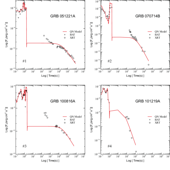
Figure 16: SGRB light-curve fits: The XRT light-curve fit for 4 SGRBs (see §  7.4). The BAT data is extrapolated to the XRT band (see Evans et al. 2010) and shown as black crosses. The XRT data is shown as open circles. The red line is the QN model.

Figure 16 is our model’s fit to light-curves of 4 selected SGRBs with the “best-fit” parameters listed in Table 4. The fits are constrained by matching the model’s $E_{\rm peak}$ to their measured $E_{\rm peak}$ (see Table 3 in D’Avanzo et al. 2014). Fitting the afterglow requires ambient density which is higher than expected for the ambient medium surrounding late evolution of NS binary merger. More detailed fits to SGRB light-curves (including flares) and spectra will be presented elsewhere.

Table 4: Preliminary fit parameters^a from the QN model for 4 SGRB sources (see §  7.4).

#	Source	$\theta_{\rm P}[\textrm{rad}]$	$\log{n_{\textrm{amb.}}}[\textrm{cm}^{-3}]$	$\log{B_{\textrm{amb.}}}[\textrm{G}]$	$n_{\textrm{pairs}}$	$\log{\epsilon_{\rm w}}$	$p$	$F_{0}^{\mathbf{b}}$	$F_{1}^{\mathbf{c}}$
1	051221A	5.00E-4	0.00	-8.00	50.00	-6.00	2.40	0.02	9.71
2	070714B	6.00E-4	1.50	-8.00	25.00	-6.00	2.60	0.11	6.73
3	100816A	6.00E-4	0.20	-8.00	60.00	-6.00	2.50	0.08	7.17
4	101219A	9.50E-4	3.50	-5.00	25.00	-6.00	2.40	0.05	1.79

^a Other parameters are set to their fiducial values (see §  7.4).
^b $F_{0}$ = location of the first filament (i.e. $R_{\rm F,in}/R_{\rm w}(t_{\rm Plat.})$).
^c $F_{1}$ = location of the last filament (i.e. $R_{\rm F,out}/R_{\rm w}(t_{\rm Plat.})$).

7.4.1 Discussion and predictions

• Light-curve variability: The PWN-“SN” is expected to be turbulent in the blow-out regime, producing irregularly spaced filaments and chaotic-looking LGRB light-curves;

• Flares are an outcome of our model (because of the secondary chunks; see §  4.2.6 and §  5.3.6) and should thus be seen in SGRBs from binary NS mergers;

• Long duration LGRBs vs SGRBs: A SGRB is thus a shortened version of a long duration ($>>1$ s) LGRB according to our model since the QN occurs days after the merger (i.e. in a more compact ejecta because of the high $B_{\rm NS}$) instead of years after the SN in the case of LGRBs. Consistent with our model, Ghirlanda et al. (2011, and references therein) find that the luminosity and the spectral properties of SGRBs resemble the first few seconds of LGRBs;

• The two-component relationships: The phenomenological Yonetoku and Amati laws should still apply to SGRBs because we still have a range in $B_{\rm NS}$ and $\theta_{\rm P}$;

• The QN-induced SN (QN-“SN”): When $t_{\rm QN}<t_{\rm QN,RS}$, following the analysis in §  5.4.1, a re-brightening of the merger’s ejecta may occur yielding a QN-“SN”. If $\zeta_{\rm QN}=10$% of the chunks’ kinetic energy is converted by the RS into accelerating the entire merger’s ejecta, the resulting ejecta’s maximum velocity is $\sim 0.75c$. However, because the ejecta is optically thin (i.e. $t_{\rm QN}>t_{\rm SLSN}$) we expect a percentage of QN-“SN” energy to be radiated on timescales of $\Delta t_{\rm QN-``SN"}\simeq R_{\rm F,out}/c\sim 5.4\ {\rm days}\times P_{\rm NS,-2.7}^{2}B_{\rm NS,14}^{-2}$ with a luminosity $L_{\rm QN-``SN"}\simeq\zeta_{\rm QN}E_{\rm QN}/\Delta t_{\rm QN-``SN"}\sim 2.1\times 10^{46}\ {\rm erg\ s}^{-1}\zeta_{\rm QN,-1}E_{\rm QN,53}P_{\rm NS,-2.7}^{-2}B_{\rm NS,14}^{2}$. Thus “SNe” associated with SGRBs will have rapidly decaying light-curves and spectra with extremely broad lines.

  There are two scenarios:

  • When the primary chunk has no RS, the outcome is a SGRB associated with a QN-“SN”.

  • When the primary chunk has RS, no SGRB results. Here, the QN-“SN” should appear as an isolated transient in no star-forming environments. In general, the spatial distribution of isolated QN-“SNe” should follow that of NS binary mergers.

  • Our preliminary fits to 4 SGRB light-curves yield parameters in favor of a no QN-“SN” scenario.

• Short duration LGRBs vs SGRBs: Both SGRBs and short duration (i.e. $<1$ s) LGRBs (see §  5.4.3) can have $t_{\rm QN}<t_{\rm QN,RS}$ but SGRBs have very low mass, so the re-brightening will not produce a Type Ic-BL SN (see §  5.4.1);

• FRBs and NS binary mergers: The interaction of QN chunks with a weakly magnetized merger ejecta should yield an FRB in a manner similar to that described for a non-blow-out SN ejecta (see §  6). Refraction (i.e. repeating FRBs) are less likely in NS binary mergers;

• The quark star radio signal: The QN compact remnant (i.e. the QS), born at time $t_{\rm SpD}$ after the merger, is rapidly rotating. The corresponding spin-down power should yield a radio signal similar to that predicted in the NS case (e.g. Nakar & Piran (2011)). The lack or presence of such a signal in SGRBs (Metzger & Bower 2014; Horesh et al. 2016) may constrain our model. However, our model for SGRBs is preliminary and key parameters remain to be explored before it can be refined;

• The GW170817 SGRB: We interpret that the SGRB associated with the GW170817 event is a no-QN event which may have resulted in a BH formation following the merger.

Our model for SGRBs is preliminary and has not been fully explored. However, a QN following a binary merger provides a framework to unify SGRBs and LGRBs.

8 General discussion and model’s limitations

8.1 A unifying model: FRBs, XRFs, XRR-GRBs, GRBs and SLSNe

X-ray Flashes (XRFs) and X-ray rich GRBs (XRR-GRBs) are in many ways very similar to GRBs except that the flux comes mostly in the 2-30 keV band (e.g. Heise et al. 2001; Barraud et al. 2003; see also Řípa & Mészáros 2016 and references therein). There is evidence that the properties of GRBS, XRR-GRBs and XRFs form a continuum (e.g. Figure 2 in Sakamoto et al. 2005) and that they have similar duration and sky distributions supporting the suggestion that they are the same phenomenon.

Figure 14 is a schematic unification of FRBs, XRFs, XRR-GRBs, LGRBs and SLSNe in our model. XRFs, XRR-GRBs and LGRBs can be unified and explained as the same phenomenon (i.e. emission induced by the interaction of the QN chunks with the PWN-SN shell) in the blow-out stage of the blow-out regime where $\epsilon_{\rm w}>\epsilon_{\rm w,WI}$ (see Table 2). One evolves from a LGRB to an XRR-GRB to finally an XRF in a continuous transition by increasing $t_{\rm QN}$ (i.e. decreasing $B_{\rm NS}$). The higher the $t_{\rm QN}$ (the lower $B_{\rm NS}$) the more extended (and less dense) the PWN-SN shell is when it is hit by the QN chunks. The viewing angle $\theta_{\rm P}$ will create overlap in properties of these phenomena. Within the LGRBs category, there is a subset of LGRBs associated with Type Ic-BL SNe occurring when $B_{\rm NS}>10^{13}$ G (see §  5.4.1) and the “SN-less” LGRB for lower NS magnetic filed (see also Table 2). At the opposite end of this classification, next to SN-LGRBs, are SLSNe which occur in a young, very dense and optically thick, PWN-SN shell. SLSNe also occur in the non-blow-out regime for $t_{\rm QN}<t_{\rm SLSN}$ while for longer time delays an FRB results.

Other noteworthy points:

• An increase in $t_{\rm QN}$ is associated with an increase in $\epsilon_{\rm w}$ and a decrease in $n_{\rm w}$. This means that as one evolves from LGRBs to XRFs, the photon peak energy on average decreases from MeVs to keVs. The lower limit (i.e. cut-off) in photon peak energy allowed in our model in the blow-out regime (i.e. in the turbulent PWN-SN case when $\epsilon_{\rm w}\geq\epsilon_{\rm w,WI}$) can be obtained from Eq. (47) by setting $\theta_{\rm P}=2/N_{\rm c}^{1/2}$ (i.e. the maximum viewing angle allowed for the primary chunk with a corresponding $f(\theta_{\rm P})=41$), $n_{\rm w}=12.6$ cm^-3 (i.e. the minimum wall density; see Eq. (24)) and $\epsilon_{\rm w}=\epsilon_{\rm w,WI}$ (as given by Eq. (66)). Eq. (47) then yields:

  $$E_{\rm\gamma,p}\sim 2\ {\rm keV}\times\zeta_{\rm WI,-2}^{1/2}\Gamma_{\rm QN,3.5}^{3}\times\left(\frac{g(p)/g(2.4)}{n_{\rm pairs,1}}\right)^{2}\ .$$ (84)

  As depicted in Figure 14, this cut-off means that in our model no bursts can occur at wavelength between the radio (i.e. the FRBs in the non-blow-out regimes) and X-ray bands;

• XRFs, which are connected with longer time delay than LGRBs, are associated with more extended and more filamentary PWN-SN resulting in more variable light-curves. In the classification suggested in Figure 14, XRR-GRBs lie between XRFs and LGRBs and should show intermediate properties (variability, frequencies etc…);

• Since flares are echoes of the prompt emission (induced by the secondary chunks), all of the points listed above should in principle apply to the flaring phases in XRFs/XRR-GRBs/LGRBs;

• The classification we suggest here assumes a narrow distribution of $\epsilon_{\rm w}$ from filament to filament in a given PWN-SN ejecta. Relaxing this assumption would allow the co-existence of $\epsilon_{\rm w}<\epsilon_{\rm w,WI}$ and $\epsilon_{\rm w}\geq\epsilon_{\rm w,WI}$ filaments in the same PWN-SN ejecta. This suggests the intriguing possibility of the co-existence of FRBs concurrently with XRFs/XRR-GRBs/LGRBs (specifically, the occurrence of FRB pulses related to filaments with $\epsilon_{\rm w}<\epsilon_{\rm w,WI}$ within light-curves of XRFs/XRR-GRBs/GRBs). This requires a wide distribution of $\epsilon_{\rm w}$ for a given PWN-SN ejecta.

8.2 FRBs/XRFs/XRR-GRBs/GRBs as probes of turbulence in PWN-SN ejecta

The classification suggested above, if verified, implies that the variability in the prompt emission (as well as in flares when present) of XRFs/XRR-GRBs/LGRBs may be a probe of the filamentary structure of PWN-SN ejecta years to decades after the SN. They could be used to help understand turbulence in PWN-SN interaction. At the other end, FRBs probe a relatively non-turbulent PWN-SN ejecta.

The spectrum of $\Delta R_{\rm F}$ and $n_{\rm F}$ derived from fits to light-curves are probably related to turbulence. The bottom panel in Figure 15 shows the distribution of the relative column density $\sum{n_{\rm F}\Delta R_{\rm F}}$ (normalized to ($n_{\rm Plat.}R_{\rm w}(t_{\rm Plat.})/12$)) when adding up all of the filaments along the line-of-sight, one for each of the 48 selected LGRBs. The resulting distribution seems to agree with the distribution of column densities resulting from the 3-Dimensional simulations of the PWN-SN shell (see Figure 8 in Blondin & Chevalier 2017).

8.3 Neutrino and Gravitational Wave signals in QNe

According to our preliminary calculations (Keränen et al. 2005; Ouyed, A. et al. 2018a, b), a QN is associated with a neutrino burst that is distinct from that of a SN. The total energy release is similar between QN and SN but the neutrino energy is higher in a QN with a neutrino-sphere temperature of $\sim 20$ MeV for a proto-QS compared to a $\sim 5$ MeV for the case of a proto-NS. Thus during the first few milliseconds that follow a QN, the neutrino signal is harder and brighter (by a factor of about $(20/5)^{4}\sim 200$) than the SN one. This translates to a peak detector count for QNe that is about a thousand times higher than the peak detector count for SNe (see Ouyed, A. (2018); Ouyed, A. et al. (2019)). Neutrino observatories, such as Super-Kamiokande-III (Ikeda et al. 2007) should in principle distinguish between the SN and QN neutrino signals. Detailed numerical simulations are required to confirm the properties of the QN neutrino signal (see details in Ouyed, A. (2018)).

Another property of a QN is its gravitational wave (GW) signal which is distinguishable from that of the preceding SN (see Appendix in Staff et al. 2012). The GW wave signal is expected to be stronger in a QN because it is a more compact explosion than a SN. If the hadronic-to-quark-matter conversion front leading to the QN is asymmetric, it should emit a gravitational wave signal with an integrated luminosity of the order of $10^{46}$-$10^{48}$ ergs or $\sim 0.01$% of binding energy of a neutron star (Staff et al. 2012). This signal should be detectable by the Advanced LIGO (LIGO Scientific Collaboration and Aasi et al. 2015) if bursts (i.e. FRBs/XRFs/XRR-GRBs/LGRBs) occur a few kpcs away. These are preliminary results and a more detailed analysis of the GW signal from a QN requires advanced numerical simulations to track the evolution of the asymmetric burning front.

The neutrino and GW signals occurring years to tens of years following the SN should be common to XRFs/XRR-GRBs/LGRBs/FRBs/SLSNe according to our model.

8.4 Model’s limitations

While our model captures key features of LGRBs and FRBs, it has some simplifying assumptions (organized by topics below) that require scrutiny before firm conclusions can be reached. For example:

• When fitting the LGRB light-curves:

  1. We have kept most parameters fixed when fitting the light-curves and spectra, varying mainly $t_{\rm QN}$ (which translates to a variation in $B_{\rm NS}$ for a fixed $P_{\rm NS}$) and the viewing angle $\theta_{\rm P}$. Nevertheless, our fits to data suggest that it may be consistent with the QN being a universal explosion (i.e. $E_{\rm QN}$ and $M_{\rm QN}$ the same from source to source). It is not unrealistic to assume that the quark deconfinement density $\rho_{\rm NS,cr.}$ (a property of Quantum-Chromo-Dynamics; e.g. Weber 2005), is universal which in principle can translate to a universal NS mass, $M_{\rm NS,cr.}$. This implies that the number of neutrons to convert to quarks is fixed during a QN and thus the energy released, $E_{\rm QN}$. On the other hand, $M_{\rm QN}$ (and thus the ejecta’s Lorentz factor $\Gamma_{\rm QN}=E_{\rm QN}/M_{\rm QN}c^{2}$) may be less straightforward since it involves complex ejection mechanisms (see discussion in Ouyed, R. & Leahy 2009). Nevertheless, a narrow distribution in $\Gamma_{\rm QN}$ peaking at $10^{3.5}$, as suggested from our fits to 48 LGRB light-curves and spectra, supports the idea of a narrow distribution in $M_{\rm QN}$ and thus a plausible universal QN explosion. At this point, we can only state that our assumption of fixed $E_{\rm QN}$ and $M_{\rm QN}$ together with the resulting successful fits to many LGRBs based on fiducial values of our parameters may be considered a self-consistency check;

  2. We assumed $\zeta_{\rm p}=1$ or that all of the swept-up proton energy in the FS is transferred to, and radiated by, leptons (electrons and pairs). This gave extreme LGRB brightness (see Eq. (65)) which can be relaxed by considering $\zeta_{\rm p}<1$. However, in this regime part of the sweeping power is transferred into the chunk’s internal energy requiring a treatment beyond the scope of this paper;

  3. We assumed that the secondary chunks ($\sim$ 6 per primary chunk in a spherical geometry) are collapsed into, and represented by, one effective secondary chunk at $\theta_{\rm S}$. Taking into account individual secondary chunks will allow for complex effects not accounted for in our model in its current version. For example, separate secondary chunks would contribute at different times and different luminosities to flares. The resulting flare will therefore be a sum of all these “mirrored” light-curves at longer times and lower fluxes than in the single secondary assumption. We should note that multiple secondaries will allow for repetitive X-ray flares as seen in some GRBs;

  4. Assuming that the chunks have reached their maximum size prior to their interaction with the wall is another simplification. In the turbulent PWN-SN ejecta presented in §  5, the wall is torn into filaments with the innermost filaments at radius $R_{\rm F}<<R_{\rm w}$ which means that chunks start interacting with the PWN-SN before they reach their maximum size (see §  2.3.2).

     • When fitting the early light-curves, the chunks are assumed bigger than they should be and this is compensated by artificially decreasing the density $n_{\rm F}$. In reality the true filament density is higher than the fit density. This can be seen in panel G in Figure 8 showing the distribution of filaments densities where a low density peak detaches itself (i.e. shifted to the left) from the main peak at $\sim 10^{3}$ cm^-3.

       This led us to introduce the fitting parameter $\alpha_{\rm F}$ (see Eq. (4) in Appendix E.2). We find $1<\alpha_{\rm F}<3$ from the fits to the 48 selected LGRBs when scaling the filament density in the pre-peak luminosity phase.

     • Past the peak luminosity, scaling the filament density using $\alpha_{\rm F}=1$ gives natural fits to the light-curves which agrees very well with our model for the constant chunk area with $n_{\rm F}\propto L_{\rm F}$ as given in Eq. (5). This suggests that once a chunk enters the densest filament (i.e. with $n_{\rm F}\sim n_{\rm w}$) it expands to its transparency radius and continues without expanding thereafter.

     • Using $A_{\rm c}(t^{\prime})$ (see Eq. (11)) instead of the maximum area $A_{\rm c,T}$, we argue, could remove the need for the $\alpha_{\rm F}$ parameter. However, a time-dependent chunk area requires re-integrating Eqs. (5) and (6) to derive $L_{\rm c,sw.}(t^{\prime})$ and $\Gamma_{\rm c}(t^{\prime})$, accordingly. This treatment is left for another paper.

  5. Fitting each LGRB is a lengthy process and we have not fully explored the degeneracy in parameters for any single LGRB. We fit 48 LGRBs and assume that their parameters distributions are somewhat representative of the whole population of LGRBs.

• When fitting the spectrum:

  1. We find it necessary to include pair creation in order to simultaneously fit the spectrum and the light-curve of a given LGRB in our model. The pair-production mechanism remains to be better understood;

  2. Assuming that the chunks have reached their maximum size prior to their interaction with the wall ignores the fact that the chunks are still thermal (i.e. emit as BBs) when they start colliding with the innermost filaments. This may modify the early spectra (see §  5.4.5) since a hybrid (BB and a Band) spectrum is the more likely outcome;

  3. In the LGRB case, we assumed an electron energy distribution with a power-law index of $p\sim 2.4$. However, since Fermi acceleration may not take place in LGRBs, because the WI is suppressed, the electrons may acquire a different distribution in energy. It remains to be shown that the convolution of distributions other than the one we adopt here for LGRBs could yield the Band function (see §  5.2);

  4. Extremely steep high-energy spectral indices (i.e. $\beta>3.0$) measured in some GRBs would require $p>5$ (i.e. $(p+1)/2>3$; see e.g. GRB 080319B listed as #31 in Table LABEL:table:lcfits in §  5.2). This also suggests an electron energy distribution other than the power-law one adopted here.

• To connect CSE emission to FRBs in the context of CCSNe:

  1. We assumed the bunching length to be set by coherence scales linked to Weibel saturated magnetic field in the shocked chunk frame. A proper treatment of the development of the instability with proper analysis of the coherence scale formation and the magnetic field amplification would require PIC simulations before particles bunching can be firmly established in our model;

  2. Ignoring pair creation altogether for the CSE gives a frequency $\nu_{\rm CSE}$ of the order of a few GHz in better agreement with data; the luminosity is independent of $n_{\rm pairs}$ (see Eq. (72)). This difference between LGRBs and FRBs in our model, in addition to understanding the pair production and suppression mechanism in itself, is unclear at the moment;

  3. To make FRBs repeat we appeal to a refracting ionized plasma (e.g. an HII region) surrounding the SN site (see Appendix G). The existence of an appropriate screen remains unclear.

• Other assumptions include:

  1. Our evaluation of the SN optical depth (see Appendix C), may be an oversimplification (see for example Bietenholz & Bartel 2017) which may affect, and shift, our estimates of the range in $t_{\rm QN}$ applicable to LGRBs and FRBs. However, this will not change our overall findings and conclusions;

  2. We have argued that a type-Ic-BL SN results when the QN chunks collide with a turbulent PWN-SN shell with filaments dense enough to trigger the RS into the chunks (see §  5.4.1). We assumed that the kinetic energy of the chunks which interacted with dense filaments is converted into kinetic energy of the surrounding PWN-SN shell material yielding a type-Ic-BL SN. However, we lack a complete physical picture of how the process occurs;

  3. We assumed that the QN ejecta fragments into chunks with single mass $m_{\rm c}$. A more realistic scenario would consist, for example, of a mass distribution close to a log-normal distribution with peak at $m_{\rm c}$, as expected in debris from explosions (e.g. the Weibull distribution; Weibull 1939; Brown & Wohletz 1995 ; see also Åström et al. 2004); The main effects are: (i) The mass of primary and secondary chunks can be significantly larger or smaller than the fiducial $10^{22.5}$ gm value. For example, if the primary chunk is much less massive than the secondary, the prompt emission may be interpreted as a precursor as discussed in §  5.4.6; (ii) The angular separation between chunks $\theta_{\rm sep.}$ would take on values that are different from the one shown in Figure 1.

9 Conclusion

Assuming a QN event occurring years to decades following the core-collapse of a massive star (e.g. a Type Ic SN as assumed in this work), we built a model capable of explaining many of the key characteristics of LGRBs and a subset of FRBs (i.e. those related to CCSNe). The time delay between the QN and the SN is the key parameter in our model since it defines the level of turbulence (thus the number of filaments) and the induced magnetization of the PWN-SN when it is sprayed by the millions of relativistic QN chunks. A shocked QN chunk emitting synchrotron radiation as it passes through successive filaments can explain the light-curves of many observed LGRBs including the flares (induced by secondary chunks) and the afterglow (from the interaction of the chunk with the medium surrounding the SN). We successfully fit the light-curves in the XRT-band (including the afterglow and the flares when present) simultaneously with the spectrum for each of the 48 LGRBs we selected. Specifically, the time-averaged fast cooling synchrotron spectra from the interaction of the chunk with successive filaments yields a Band-like spectrum which for a given burst can be fit simultaneously with the resulting light-curve.

In our model, the Yonetoku and Amati laws are not fundamental but are instead phenomenological because the LGRB properties (i.e. $L_{\rm iso,peak},E_{\rm peak}$ and $E_{\rm iso}$) depend on multiple physical parameters, which each have a limited range of scatter.

The FRBs described here result from the interaction of QN chunks with a non-turbulent or a weakly-turbulent (and thus weakly magnetized) PWN-SN shell with conditions prone to the development of the Weibel instability in the shocked chunk frame. The coherence length associated with the Weibel amplified magnetic field in the shocked chunk frame leads to electron and pair bunching triggering coherence synchrotron emission, in contrast to the LGRB case. The resulting frequency, luminosity and timescale are consistent with those of observed FRBs.

Besides the limitations listed in §  8.4, our model relies on the feasibility of a delayed explosive transition of a massive NS to a QS years to decades following the SN explosion of a massive star. While such a transition is already hinted at by analytical (e.g. Keränen et al. 2005; Vogt et al. 2004; Ouyed, R. & Leahy 2009) and by one-dimensional numerical simulations (Niebergal et al. 2010; Ouyed, A. et al. 2018a, b; see also Ouyed, A. et al. 2019), detailed multi-dimensional simulations are required to prove or disprove our working hypothesis (Niebergal 2011; Ouyed, A. 2018). Furthermore, a full treatment of the interaction between the relativistic QN ejecta and the turbulent and non-turbulent PWN-SN shell would require detailed hydrodynamical simulations beyond the scope of this paper. Despite these limitations, our model seems successful at capturing key properties of LGRBs and FRBs and at unifying them with other related phenomena such as XRFs, XRR-GRBs and SLSNe.

If our model is the correct representation of these phenomena, it can be used to probe the structure and physics of collisionless relativistic shocks and of the Weibel instability and related coherence lengths. The connection between FRBs and UHECRs as we suggest here (see §  7.2) means that FRBs can also be a vehicle to understanding Fermi acceleration.

Our model and findings suggest that : (i) a catastrophic event (i.e. the QN) is behind LGRBs (including SGRBs) and some FRBs; (ii) NSs born with periods in the range $1.5\ {\rm ms}<P_{\rm NS}\leq P_{\rm NS,cr.}$ and with mass $M_{\rm NS}\geq M_{\rm NS,cr.}$ can explode as QNe releasing $\sim 10^{53}$ ergs in kinetic energy; (iii) spontaneous strange-quark nucleation can occur during quark deconfinement (e.g. Bombaci et al. 2009) induced by spin-down in massive NSs.

Confirming the QN as the engine driving LGRBs and FRBs means that other implications of QNe to Cosmology (e.g. to re-ionization (Ouyed, R. et al. 2009c) and to type Ia SNe calibration (Ouyed, R. et al. 2014, 2015d)), to binary evolution (Ouyed, R. et al. 2016, 2018a) and to AXPs/SGRs (e.g. Ouyed, R. et al. 2007a, b, 2018b) warrant further studies.

10 Acknowledgements

This research is supported by operating grants from the National Science and Engineering Research Council of Canada (NSERC). This work made use of data supplied by the UK Swift Science Data Centre at the University of Leicester.

Appendix A Reference frames

Here we list the three reference frames involved: (i) the chunk’s (i.e. co-moving) frame where the quantities are primed (the subscript “c” stands for “chunk” and is used to denote chunk’s parameters); (ii) the exploding NS frame (also the GRB cosmological rest frame) where quantities are unprimed; (iii) the observer’s frame denoted by the superscript “obs.” in which quantities are angle dependent. The Doppler factor is $D_{\rm c}(\Gamma_{\rm c}(t^{\prime}),\theta_{\rm c})=1/(\Gamma_{\rm c}(t^{\prime})(1-\beta_{\rm c}(t^{\prime})\cos{\theta_{\rm c}}))$ where $\Gamma_{\rm c}(t^{\prime})$ is the chunk’s Lorentz factor, $\beta_{\rm c}(t^{\prime})=v_{\rm c}(t^{\prime})/c$ with $v_{\rm c}(t^{\prime})$ the chunk’s speed and $\theta_{\rm c}$ the chunk’s viewing angle. The chunk’s initial Lorentz factor is $\Gamma_{\rm c}(0)=\Gamma_{\rm QN}$. The transformation from the local NS frame to the chunk’s frame is given by $dt=\Gamma_{\rm c}(t^{\prime})dt^{\prime}$ while the transformation from the chunk’s frame to the observer’s frame (where the emitted light is being observed) are $dt^{\rm obs.}=(1+z)dt^{\prime}/D_{\rm c}(\Gamma_{\rm c}(t^{\prime}),\theta_{\rm c})$, $\nu^{\rm obs.}=D_{\rm c}(\Gamma_{\rm c}(t^{\prime}),\theta_{\rm c})\nu^{\prime}/(1+z)$ where $z$ is the source’s redshift. The NS frame and the observer frame share the same spatial co-ordinates, except for the $(1+z)$ factor, but not time which is subject to the additional Doppler factor.

Appendix B Some properties of the neutron-rich ultra-relativistic QN ejecta

B.1 Chunks angular distribution and statistics

The QN causes the outermost NS crust to be ejected, which then breaks into $N_{\rm c}=10^{6}$ chunks, each with $\Gamma_{\rm c}(0)=\Gamma_{\rm QN}=10^{3.5}$ and equally spaced in solid angle centered on the explosion site. I.e. many bright small pieces ejected radially outward from the explosion center.

For a distribution of $N_{\rm c}$ chunks that is uniform in solid angle we have $dN_{\rm c}/d\Omega=const.=N_{\rm c}/4\pi$ with $d\Omega=2\pi\sin{\theta}d\theta$ so that

$$\frac{dN_{\rm c}}{d\theta}=\frac{N_{\rm c}}{2}\sin{\theta}\simeq\frac{N_{\rm c}}{2}\theta\ ,$$ (1)

where the last expression applies the small angle approximation; i.e. $N_{\rm c}(\theta)\propto\theta^{2}$. We note the following characteristics of the distribution:

(i) The solid angle covered by each chunk is given by $\pi\theta_{\rm c}^{2}=4\pi/N_{\rm c}$ . This gives an angular separation between chunks of $\theta_{\rm sep.}=2\theta_{\rm c}=4/N_{\rm c}^{1/2}=4\times 10^{-3}/N_{\rm c,6}^{1/2}$. For our fiducial value of $\Gamma_{\rm c}=10^{3.5}$, the angular separation between chunks is about $12.6/\Gamma_{\rm c}$ (with $\Gamma_{\rm c}=\Gamma_{\rm QN}$ initially). Each chunk emits radiation into a narrow beam with half angle $\simeq 1/\Gamma_{\rm c}$ (i.e. a beam fullwidth of $2/\Gamma_{\rm c}=6.3\times 10^{-4}/\Gamma_{\rm c,3.5}$) which is about 1/6 of the angular spacing between chunks. This means emission pattern on the sky is $\sim 10^{6}$ narrow radial beams, one for each chunk, spaced over the whole sky;

(ii) The chunk aligned most closely toward to the observer is call the primary chunk. The observed mean angle for the primary chunk is $\bar{\theta}_{\rm P}=\int_{0}^{\theta_{\rm c}}2\pi\theta^{2}d\theta/\int_{0}^{\theta_{\rm c}}2\pi\theta d\theta=(2/3)\theta_{\rm c}=(4/3)/N_{\rm c}^{1/2}=1.3\times 10^{-3}N_{\rm c,6}^{-1/2}$ which is close to $\sim 4/\Gamma_{\rm c}$;

(iii) There are 6 peripheral chunks we refer to as secondary chunks. We define the viewing angle of the secondary chunks as $\theta_{\rm S}$ with $\theta_{\rm S}(\theta_{\rm P})=2\theta_{\rm c}-\theta_{\rm P}$ which has a mean value of $\bar{\theta}_{\rm S}=\int_{\theta_{\rm c}}^{2\theta_{\rm c}}2\pi\theta^{2}d\theta/\int_{\theta_{\rm c}}^{2\theta_{\rm c}}2\pi\theta d\theta\simeq(14/9)\theta_{\rm c}=(28/9)/N_{\rm c}^{1/2}=3.1\times 10^{-3}N_{\rm c,6}^{-1/2}$ which is close to $\sim 10/\Gamma_{\rm c}\sim 3.1\times 10^{-3}/\Gamma_{\rm c,3.5}$;

(iv) We refer to emission with $\theta_{\rm P}>2/\Gamma_{\rm c}$ as “off-axis” The “off-axis” solid angle is about 36 times the on-axis solid angle. I.e. there will be one bright burst for every $\sim 36$ faint bursts. For an observer, this means most bursts will be “off-axis”.

B.2 The QN ejecta as an r-process site

The extremely neutron-rich, relativistically expanding, QN ejecta is converted to unstable r-process material in a few milliseconds (Jaikumar et al. 2007; Kostka et al. 2014b, c; Kostka 2014). Figures 5 and 6 in Kostka et al. (2014c, see also ) show examples of the final composition of the expanding QN ejecta. The different Lorentz factor, $\Gamma_{\rm QN}$, of the QN ejecta, correspond to different expansion timescales thus the differences in the final abundances. For $M_{\rm QN}<10^{-4}M_{\odot}$ (i.e. $\Gamma_{\rm QN}>10^{3}$), the abundances are dominated by elements with atomic weight $A<100$. We adopt a chunk’s opacity of $\kappa_{\rm c}=0.1$ cm² gm^-1 in this work since Lanthanides (which would otherwise yield a much higher opacity; see Kasen et al. 2013; Tanaka & Hotokezaka 2013) are not present in large quantities in the QN r-process yield for low QN mass ejecta.

The $\beta$-decay luminosity in the chunk’s frame can be defined by the following equations (e.g. Korobkin et al. 2012)

$$L_{\rm c,\beta}^{\prime}(t^{\prime}) =2\times 10^{18}\ {\rm erg\ g}^{-1}\ {\rm s}^{-1}\times\epsilon_{\rm th.,0.5}\times m_{\rm c}\times rp(t^{\prime})$$ (2)

$$rp(t^{\prime}) =\left(\frac{1}{2}-\frac{1}{\pi}\arctan{\left(\frac{t^{\prime}-t_{\rm F}^{\prime}}{0.11}\right)}\right)^{1.3}\ ,$$ (3)

where $t_{\rm F}^{\prime}$ which of the order of a second is the freeze-out timescale and $\epsilon_{\rm th.,0.5}=\epsilon_{\rm th.}/0.5$ the percentage of $\beta$-decay energy which thermalizes in the chunk in units of 0.5.

When $t^{\prime}$ exceeds a few times the freeze-out time (the case in our model) the $\beta$-decay contribution can be expressed as (e.g. Li-Xin & Paczyński 1998; Metzger et al. 2010b)

$$L_{\rm c,\beta}^{\prime}(t^{\prime})\sim 9\times 10^{38}\ {\rm erg\ g}^{-1}\ {\rm s}^{-1}\times m_{\rm c,22.5}\times\left(\frac{t^{\prime}}{1\ {\rm s}}\right)^{-1.3}\ .$$ (4)

B.3 The chunk’s sweeping luminosity

The evolution in the chunk’s rest frame of the sweeping luminosity $L_{\rm c,sw.}^{\prime}(t^{\prime})$ and of the Lorentz factor $\Gamma_{\rm c}(t^{\prime})$ are given by the two following fundamental equations

$$L_{\rm c,sw.}^{\prime}(t^{\prime}) =E_{\rm p}(t^{\prime})\times A_{\rm c}(t^{\prime})\times(\Gamma_{\rm c}(t^{\prime})n_{\rm amb.})\times\beta_{\rm c}c$$ (5)

$$-\frac{d\Gamma_{\rm c}(t^{\prime})}{\Gamma(t^{\prime})^{2}} =\frac{4A_{\rm c}(t^{\prime})\times\rho_{\rm amb.}\times(\beta_{\rm c}c\times(\Gamma_{\rm c}(t^{\prime})dt^{\prime}))}{3m_{\rm c}}\ ,$$ (6)

where hereafter $\beta_{\rm c}=v_{\rm c}/c=1$. The above is for a chunk of mass $m_{\rm c}$ and area $A_{\rm c}(t^{\prime})$ sweeping protons and electrons in an ambient medium of baryon number density $n_{\rm amb.}$. These equations assume is the radiative case and $\Gamma_{\rm c}>>1$ (e.g. Pe’er 2012 and references therein).

The unprimed quantities are in the NS’s frame, with $dt=\Gamma(t^{\prime})dt^{\prime}$. The adiabatic index of the swept-up material is taken to be 4/3 and $E_{\rm p}(t^{\prime})=\zeta_{\rm p}\Gamma_{\rm c}(t^{\prime})m_{\rm p}c^{2}$ is the the fraction of proton energy transferred to electron-positron pairs. We take $\zeta_{\rm p}=1$ for simplicity, effectively assuming efficient thermalization of dissipated kinetic energy in the shocks. This means that electrons (and positrons) are accelerated to a Lorentz factor of $\gamma_{\rm e}\sim(1/2n_{\rm pairs})\times\Gamma_{\rm c}(t^{\prime})m_{\rm p}/m_{\rm e}$. Here $n_{\rm pairs}$ is the number of paris created per proton (see §  4.2.5). This is representative of the radiative case (where most of the swept energy is promptly radiated) and is associated in our model with the regime where the chunk is optically thin (see §  2.3.2). These simplifying assumptions allow us to provide analytical solutions in our model. In particular, for a constant sweeping area $A_{\rm c}(t^{\prime})=A_{\rm c,T}$ (see Eq. (2)), Eq. (6) becomes

$$d\left(\frac{\Gamma_{\rm c}(0)^{2}}{\Gamma_{\rm c}(t^{\prime})^{2}}\right)=d\left(\frac{t^{\prime}}{t_{\Gamma}^{\prime}}\right)\ ,$$ (7)

with $t_{\Gamma}^{\prime}$ and the solution, $\Gamma_{\rm c}(t^{\prime})$, to equation above given in Eqs. (6) and (4), respectively.

B.4 QN chunks inside a PWN

Since the QN involves the explosion of a NS, it is natural to consider the evolution of the QN ejecta inside a PW bubble. Before the chunks collide with the PWN-SN shell, the density is such that the sweeping luminosity is dwarfed by heating from $\beta$-decay; i.e. $L_{\rm c,sw.}(t)<<L_{\beta}(t)$. The time evolution of the chunk’s cross-section area $A_{\rm c}(t)$ and temperature $T_{\rm c}(t)$ during the time that the chunk is optically thick (i.e. when $A_{\rm c}(t^{\prime})<A_{\rm c,T}$ where $A_{\rm c,T}$ is the area of the chunk when it becomes optically thin; see Eq. (2)) is found from

$$A_{\rm c}(t^{\prime}) =\pi(R_{\rm c,0}^{\prime}+c_{\rm s,c}^{\prime}t^{\prime})^{2}$$ (8)

$$4A_{\rm c}(t^{\prime})\sigma_{\rm SB}{T^{\prime}}^{4} =L_{\beta}^{\prime}(t^{\prime})+L_{\rm c,sw.}^{\prime}(t^{\prime})\sim L_{\rm c,\beta}^{\prime}(t^{\prime})\ ,$$ (9)

where $c_{\rm s,c}^{\prime}=\sqrt{\gamma_{\rm ad.,c}\frac{k_{\rm B}T^{\prime}}{\mu_{\rm c}m_{\rm H}}}$ is the sound speed in the chunk and $R_{\rm c,0}^{\prime}$ is the chunk’s initial radius. The constants are the Boltzmann constant $k_{\rm B}$, the hydrogen mass $m_{\rm H}$ and, the Stefan-Boltzmann constant $\sigma_{\rm SB}$. The chunk’s adiabatic index is taken as $\gamma_{\rm ad.,c}=5/3$, and the chunk’s mean molecular weight (for heavy composition) is $\mu_{\rm c}\simeq 2$.

Analytical solutions can then be found for timescales relevant to the QN-SN interaction, $t^{\prime}>>R_{\rm c,0}^{\prime}/c_{\rm s,c}^{\prime}$ and $t^{\prime}>t_{\rm A}^{\prime}$. In this case, the $\beta$-decay contribution is given by Eq. (4) which allows us to solve for:

$$k_{\rm B}T_{\rm c}^{\prime}(t^{\prime}) \sim 0.6\ {\rm keV}\ m_{\rm c,22.5}^{1/5}\times(t^{\prime})^{-3.3/5}$$ (10)

$$A_{\rm c}^{\prime}(t^{\prime}) \sim 1.5\times 10^{15}\ {\rm cm}^{2}\ m_{\rm c,22.5}^{1/5}\times(t^{\prime})^{6.7/5}\ .$$ (11)

Setting $A_{\rm c}(t_{\rm T}^{\prime})=A_{\rm c,T}$ gives a critical time which defines the end of the chunk’s optically thick expansion and the start of the optically thin regime, where the chunk stops expanding. This time is

$$t_{\rm T}^{\prime}\simeq 4.3\times 10^{4}\ {\rm s}\times m_{\rm c,22.5}^{4/6.7}\kappa_{c,-1}^{5/6.7}\ .$$ (12)

The above is an upper limit on the time it would take the expanding chunk to reach transparency, because it only takes into account heating from $\beta$-decay. Including heating from sweeping yields higher temperatures which makes the chunk expand faster and yields a smaller transparency time.

In the NS frame the transparency time is $t_{\rm T}=\Gamma_{\rm QN}t_{\rm T}^{\prime}$ corresponding to a distance from the NS of

$$R_{\rm T}=ct_{\rm T}<4.1\times 10^{18}\ {\rm cm}\times m_{\rm c,22.5}^{4/6.7}\kappa_{\rm c,-1}^{5/6.7}\Gamma_{\rm QN,3.5}\ .$$ (13)

Appendix C The SN ejecta’s optical depth

The optical depth of the SN ejecta is $\tau_{\rm SN}=\int_{R_{\rm w}}^{R_{\rm SN}}\sigma_{\rm Th.}n_{\rm e,SN}dr=\tau_{\rm SN,inner}+\tau_{\rm SN,outer}$, where $\sigma_{\rm Th.}$ is the Thomson optical depth and $n_{\rm e,SN}=\rho_{\rm SN}/m_{\rm H}$, with

$$\tau_{\rm SN,inner} =\int_{R_{\rm w}}^{R_{\rm Plat.}}\sigma_{\rm Th.}n_{\rm e,Plat.}dr$$ (1)

$$=\sigma_{\rm Th.}n_{\rm e,Plat.}R_{\rm Plat.}\left(1-\frac{R_{\rm w}}{R_{\rm Plat.}}\right)$$

and

$$\tau_{\rm SN,outer} =\int_{R_{\rm Plat.}}^{R_{\rm SN}}\sigma_{\rm Th.}n_{\rm e,SN}dr$$ (2)

$$=\int_{R_{\rm Plat.}}^{R_{\rm SN}}\sigma_{\rm Th.}n_{\rm e,Plat.}\left(\frac{R_{\rm Plat.}}{r}\right)^{-n}dr$$

$$\simeq\sigma_{\rm Th.}n_{\rm e,Plat.}R_{\rm Plat.}\times\frac{1}{8}\left(1-\left(\frac{R_{\rm SN}}{R_{\rm Plat.}}\right)^{-8}\right)\ .$$

where $n_{\rm e,Plat.}=\rho_{\rm e,Plat.}/m_{\rm H}=At^{-3}/m_{\rm H}$ and $R_{\rm Plat.}=v_{\rm t}t$. Adding Eqs. (1) and (2) for $R_{\rm SN}>>R_{\rm Plat.}$ yields

$$\tau_{\rm SN}\sim(3.15\times 10^{15}t^{-2})\times{E_{\rm SN,51}}^{-1}M_{\rm SN,34}^{2}\ .$$ (3)

The conditions $\tau_{\rm SN}<1$ yields

$$t_{\rm QN}>t_{\rm SLSN}=1.8\ {\rm years}\times{E_{\rm SN,51}}^{-1/2}M_{\rm SN,34}\ .$$ (4)

Appendix D The thick wall case

For the thick wall case, the forward shock (FS) Lorentz factor varies in time as $\Gamma_{\rm FS}(t^{\prime})\simeq\Gamma_{\rm c}(t^{\prime})$ with $\Gamma_{\rm c}(0)=\Gamma_{\rm QN}$. Thus the main differences between the thin wall and thick wall cases are: (i) integrating time variable quantities that depend on the decreasing Lorentz factor $\Gamma_{\rm c}(t^{\prime})$); (ii) time-averaging of quantities such as the time-dependent photon peak energy and luminosity; (iii) setting the typical GRB duration, in the NS frame, to be $3t_{\Gamma}$.

The peak frequency of a single chunk is averaged over time, weighted by photon number:

$$\bar{E}_{\rm\gamma,p}=\frac{\int_{0}^{t_{\rm w}}E_{\rm\gamma,p}(t)N(t)dt}{\int_{0}^{t_{\rm w}}N(t)dt}\ ,$$ (1)

where the photon rate is $N(t)=L(t)/h\nu\propto\Gamma_{\rm FS}^{6}/\Gamma_{\rm FS}\propto\Gamma_{\rm FS}^{5}(t)$ so that

$$\bar{E}_{\rm\gamma,p}=\frac{\int_{0}^{t_{\rm w}}E_{\rm\gamma,p}(t)\Gamma(t)^{5}dt}{\int_{0}^{t_{\rm w}^{\rm obs.}}\Gamma(t)^{5}dt}\ .$$ (2)

The peak luminosity occurs at $\Gamma_{\rm c}(0)=\Gamma_{\rm QN}$, i.e.

$$L_{\rm GRB,p}=D(\Gamma_{\rm QN},\theta_{\rm P})^{4}{L^{\prime}}_{\rm c,sw.}(0)\ ,$$ (3)

where the chunk’s sweeping luminosity is $L^{\prime}_{\rm c,sw.}(t^{\prime})=C_{1}^{\prime\prime}\times\Gamma_{\rm c}(t^{\prime})^{2}n_{\rm w}\kappa_{\rm c}$ ($C_{1}^{\prime\prime}$ is a constant; see Eq. (5)) with $\Gamma_{\rm c}(t^{\prime})=\Gamma_{\rm c}(0)/(1+t^{\prime}/t_{\Gamma}^{\prime})^{1/2}$ (see Eq. (6)).

The isotropic energy $E_{\rm GRB}$ from a single chunk is:

$$E_{\rm GRB}=\int_{0}^{t_{\rm w}^{\prime}}D(\Gamma_{\rm c}(t^{\prime}),\theta_{c})^{3}L_{\rm c,sw.}^{\prime}(t^{\prime})dt^{\prime}=C_{1}^{\prime\prime}\times 2^{3}n_{\rm w}\kappa_{\rm c}\int_{0}^{t_{\rm w}^{\prime}}\frac{\Gamma_{\rm c}(t^{\prime})^{5}}{(1+(\Gamma_{\rm c}(t^{\prime})\theta_{\rm c})^{2})^{3}}dt^{\prime}\ ,$$ (4)

where we made use of $D(\Gamma_{\rm c}(t^{\prime}),\theta_{\rm c})=2\Gamma_{\rm c}(t^{\prime})/(1+(\Gamma_{\rm c}(t^{\prime})\theta_{\rm c})^{2})$. One can show that

$$\frac{dt^{\prime}}{t_{\Gamma}^{\prime}}=-2\left(\frac{\Gamma_{\rm c}(0)}{\Gamma_{\rm c}}\right)^{2}\frac{d\Gamma_{\rm c}}{\Gamma_{\rm c}}\ ,$$ (5)

so the integral above becomes

$$E_{\rm GRB}=-C_{1}^{\prime\prime}\times 2^{4}\Gamma_{\rm c}(0)^{2}n_{\rm w}\kappa_{\rm c}t_{\Gamma}^{\prime}\int_{\Gamma_{\rm c}(0)}^{\Gamma_{\rm c,F}}\frac{\Gamma_{\rm c}^{2}}{(1+(\Gamma_{\rm c}\theta_{\rm c})^{2})^{3}}d\Gamma_{\rm c}\ ,$$ (6)

where $\Gamma_{\rm c,F}$ is the chunk’s Lorentz factor at the exit of the filament.

Since $t_{\Gamma}^{\prime}=C_{2}^{\prime\prime}\times(n_{\rm w}\Gamma_{\rm c}(0)^{2}\kappa_{\rm c})^{-1}$ (see Eq. (6)) we can rewrite the above as

$$E_{\rm GRB}=-C_{1}^{\prime\prime\prime}\times 2^{4}\times\int_{\Gamma_{\rm c}(0)}^{\Gamma_{\rm c,F}}\frac{\Gamma_{\rm c}^{2}}{(1+(\Gamma_{\rm c}\theta_{\rm c})^{2})^{3}}d\Gamma_{\rm c}\ ,$$ (7)

with $C_{1}^{\prime\prime\prime}=C_{1}^{\prime\prime}C_{2}^{\prime\prime}$.

Appendix E Light-curve and spectrum simulation algorithms

As described in section §  5, the variability of each LGRB light-curve is determined by the spatial (location/thickness) and density distributions of the filaments. In order to successfully model a specific LGRB light-curve, we must therefore determine these distributions which will be dependent on our fitting parameters.

E.1 Filament location and thickness generation

The algorithm for finding the location and thickness of each filament (using observed data points) during a simulation is given below. It gives a good approximation to the observed light-curves:

1. Create a first “filament”, $F_{0}$, to represent the outer edge of the pulsar wind bubble inside of which the density is set to 0. Set its position, $d_{0}$ to 0.

2. For each subsequent data point, $i$, in the observed set (i.e. light-curve) do the following:

   1. Transform the point time, $t_{i}^{\textrm{obs}}$, to the rest frame time, $t_{i}^{\prime}$, of the chunk:

      $$t^{\prime}_{i}=\frac{(t_{i}^{\textrm{obs}}-t_{i-1}^{\textrm{obs}})D(\Gamma_{i,0},\theta_{\rm c})}{(1+z)}+t_{i-1}^{\prime}$$ (1)

      where $t_{i-1}^{\rm obs}$ and $t^{\prime}_{i-1}$ is the observed and chunk frame time, respectively, when the chunk entered the previous filament ($F_{i-1}$); here $\Gamma_{i,0}$ is the value of the Lorentz factor when the chunk exits the previous filament.

   2. Calculate the distance, in the NS frame, the chunk traveled in this time:

      $$\Delta d_{i}=2c\Gamma_{i,0}t_{\Gamma_{i}}^{\prime}\left[\sqrt{1+\frac{t_{i}^{\prime}}{t_{\Gamma_{i}}^{\prime}}}-\sqrt{1+\frac{t_{i-1}^{\prime}}{t_{\Gamma,i}^{\prime}}}\right]$$ (2)

      Where $t_{\Gamma_{i}}^{\prime}$ is given by Eq. (6). Set the end position of our filament, $F_{i}$, to:

      $$d_{i,1}=d_{i,0}+\Delta d_{i}\ .$$ (3)

   3. If $\Delta d_{i}$ is greater than $\Delta R_{\rm F,max.}=R_{\rm w}(t_{\rm Plat.})/3$ (the maximum filament’s thickness), create a “gap” filament, $F_{g}$ with $n_{g}=0$ and adjust $d_{i,1}$ of $F_{i}$ accordingly. In this way, no filament can exceed a width of $R_{\rm w}/12$. Effectively, the filament’s thickness is $\Delta R_{\rm F_{i}}={\rm Min}[\Delta d_{i},\Delta R_{\rm F,max.}]$.

   4. Create a new filament, $F_{i+1}$, with its start position at $d_{i+1,0}=d_{i,1}=d_{i,0}+\Delta d_{i}$.

3. Create a final “filament” with infinite thickness, $F_{\textrm{amb.}}$, to represent the ambient medium (e.g. ISM or the low density SN ejecta overlaying the wall) with density $n_{\textrm{amb.}}$ and magnetic field $B_{\textrm{amb.}}$.

E.2 Filament density generation

Instead of fitting a large number of individual filament densities (about a hundred per LGRB), we chose to fit the peak luminosity (assigned a density $n_{\rm w}$) of the selected LGRB then scale all other filament densities $n_{\rm F}$ using the following power-law

$$n_{\rm F}=\begin{cases}n_{\rm w}\times\left(\frac{L_{\rm F}}{L_{\rm GRB,p}}\right)^{\alpha_{\rm F}}\,&\text{for\ }t^{\rm obs.}<t^{\rm obs.}_{\rm p}\\ n_{\rm w}\times\left(\frac{L_{\rm F}}{L_{\rm GRB,p}}\right)\,&\text{for\ }t^{\rm obs.}>t^{\rm obs.}_{\rm p}\ .\end{cases}$$ (4)

Here, $t^{\rm obs.}_{\rm p}$ is the location of the peak luminosity, $L_{\rm GRB,p}$, in the light-curve. The parameter $\alpha_{\rm F}>0$ is a constant for each burst and is a consequence of our assumption of constant chunk area (given by Eq. (2)) which is invalid in the pre-peak luminosity phase during the interaction with the filaments (see discussion in §  8.4). For $t^{\rm obs.}>t^{\rm obs.}_{\rm p}$, $\alpha_{\rm F}=1$ gives good fits to light-curves and agrees well with the maximum chunk’s area regime where $n_{\rm F}\propto L_{\rm GRB}$ (see Eq. (5)).

E.3 Light-curve generation

The observed light-curve for the GRB is calculated by the following algorithm:

1. Generate a list of time points in the rest frame of the chunk. The simulation uses 500 evenly spaced time intervals in log scale between $-3\leq\log(t^{\prime})\leq 10$. In order to assure adequate sampling of each filament, we also calculate emission for 100 equally spaced time intervals in log scale between $\log(t^{\prime}_{0})\leq\log(t^{\prime})\leq\log(t^{\prime}_{1})$ where $t^{\prime}_{0}$ and $t^{\prime}_{1}$ are the time the chunk enters and exits the filament, respectively. Each filament is resolved into 100 time-steps in order to capture the slowing down of the chunk within a filament.

2. For the primary chunk in the simulation, step through the time points and calculate : The corresponding observed time, and the observed luminosity. The observed time for the ith time point is calculated as:

   $$t^{\textrm{obs}}_{i}=\frac{(1+z)(t^{\prime}_{i}-t^{\prime}_{i-1})}{D(\Gamma_{\rm c},\theta_{\rm c})}+t^{\textrm{obs}}_{i-1}\ .$$ (5)

   Eq. (5) above is the inverse of Eq. (1). However, the observed time in Eq. (5) refers to time in the observer’s frame based on our model while $t^{obs}$ in Eq. (1) means the actual observed time (i.e. for each data point) for the light-curve being fit.

   The luminosity in the XRT band ($0.3\leq E_{\gamma}^{\textrm{obs}}\leq 10$ keV) is calculated as:

   $$\begin{split}L^{\textrm{obs}}(E_{\gamma,0}^{\textrm{obs}},E_{\gamma,1}^{\textrm{obs}})&=(1+z)D(\Gamma_{\rm c},\theta_{\rm c})^{4}L^{\prime}(E_{\gamma,0}^{\prime},E_{\gamma,1}^{\prime})\\ L^{\prime}(E_{\gamma,0}^{\prime},E_{\gamma,1}^{\prime})&=C_{\rm XRT}\int_{E_{\gamma,0}^{\prime}}^{E_{\gamma,1}^{\prime}}{L^{\prime}(E_{\gamma}^{\prime})dE_{\gamma}}^{\prime}\ .\end{split}$$ (6)

   With

   $$E_{\gamma}^{\prime}=\frac{E_{\gamma}}{D(\Gamma_{\rm c},\theta_{\rm c})}=\frac{(1+z)E_{\gamma}^{\textrm{obs}}}{D(\Gamma_{\rm c},\theta_{\rm c})}$$ (7)

   and an XRT bolometric correction (the BAT emission in the fit light-curve was converted to XRT band in Evans et al. (2010))

   $$C_{\rm XRT}=\frac{L^{\prime}_{\textrm{c., sw.}}}{L^{\prime}(E_{\gamma,0}^{\prime},E_{\gamma,1}^{\prime})}\ ,$$ (8)

   is a constant with the chunk’s sweeping luminosity $L^{\prime}_{\textrm{c, sw.}}$ given by Eq. (5) being the bolometric luminosity. The fast and slow cooling regimes are defined each by their luminosity density given in the following equations

   $$L^{\prime}(E_{\gamma}^{\prime})=\begin{cases}L^{\prime}_{\textrm{slow}}(E_{\gamma}^{\prime}),&\text{if }E_{\gamma,p}^{\prime}\leq E_{\gamma,c}^{\prime}\\ L^{\prime}_{\textrm{fast}}(E_{\gamma}^{\prime}),&\text{if }E_{\gamma,p}^{\prime}>E_{\gamma,c}^{\prime}\end{cases}$$ (9)

   $$L^{\prime}_{\textrm{slow}}(E_{\gamma}^{\prime})=C_{\rm XRT}\ {\rm erg\ s^{-1}\ keV^{-1}}\times\begin{cases}(E_{\gamma}^{\prime}/E_{\gamma,p}^{\prime})^{1/3},&\text{if }E_{\gamma}^{\prime}<E_{\gamma,p}^{\prime}\\ (E_{\gamma}^{\prime}/E_{\gamma,p}^{\prime})^{-(p-1)/2},&\text{if }E_{\gamma,p}^{\prime}\leq E_{\gamma}^{\prime}\leq E_{\gamma,c}^{\prime}\\ (E_{\gamma,c}^{\prime}/E_{\gamma,p}^{\prime})^{-(p-1)/2}(E_{\gamma}^{\prime}/E_{\gamma,c}^{\prime})^{-p/2},&\text{if }E_{\gamma}^{\prime}>E_{\gamma,c}^{\prime}\par\end{cases}$$ (10)

   $$L^{\prime}_{\textrm{fast}}(E_{\gamma}^{\prime})=C_{\rm XRT}\ {\rm erg\ s^{-1}\ keV^{-1}}\times\begin{cases}(E_{\gamma}^{\prime}/E_{\gamma,c}^{\prime})^{1/3},&\text{if }E_{\gamma}^{\prime}<E_{\gamma,c}^{\prime}\\ (E_{\gamma}^{\prime}/E_{\gamma,c}^{\prime})^{-1/2},&\text{if }E_{\gamma,c}^{\prime}\leq E_{\gamma}^{\prime}\leq E_{\gamma,p}^{\prime}\\ (E_{\gamma,p}^{\prime}/E_{\gamma,c}^{\prime})^{-1/2}(E_{\gamma}^{\prime}/E_{\gamma,p}^{\prime})^{-p/2},&\text{if }E_{\gamma}^{\prime}>E_{\gamma,p}^{\prime}\par\end{cases}$$ (11)

   In the above $E_{\gamma,c}^{\prime}=E_{\gamma,c}/D(\Gamma_{\rm c},\theta_{\rm c})$ and $E_{\gamma,p}^{\prime}=E_{\gamma,p}/D(\Gamma_{\rm c},\theta_{\rm c})$ with $E_{\gamma,c}$ and $E_{\gamma,p}$ given by Eqs. (46) and (47), respectively.

3. Create observed time bins between $t^{\textrm{obs}}$ = 0 and the last BAT time point in the observed data. The width of each bin during the prompt is set to 64 ms, and 100 s during the afterglow.

4. For each time bin ($t^{\textrm{obs}}_{\rm bin}$) created in step 3, add the calculated observed flux ($F^{\textrm{obs}}=D(\Gamma_{\rm c},\theta_{\rm c})^{4}L_{\rm c,sw.}^{\prime}/(4\pi d_{\rm L}^{2})$) for each chunk. If the chunk does not have a calculated flux for the $t^{\textrm{obs}}_{\rm bin}$, use linear interpolation in time to find it.

E.4 Spectrum

The final spectrum is created between energies of 0.2 and $10^{6}$ keV (in the observer’s frame) by taking an average of spectra sampled at each observed time point generated for the light-curve (see step 1 in §  E.3; i.e. using the same sample points as in light-curve generation). The algorithm for creating a single spectrum at $t^{\textrm{obs}}$ is the following (using the primary chunk):

1. For the primary chunk in our simulation, generate an observed spectrum at $t^{\textrm{obs}}$:

2. For each energy in our observed spectrum, $0.2\leq E_{\gamma}^{\textrm{obs}}\leq 10^{6}$ keV, calculate the observed flux density:

   $$F^{\textrm{obs}}(E_{\gamma}^{\textrm{obs}})=D(\Gamma_{\rm c},\theta_{\rm c})^{3}(1+z)\frac{L^{\prime}(E_{\gamma}^{\prime})}{4\pi d_{\rm L}^{2}}$$ (12)

   which is the observed flux at $E_{\gamma}^{\prime}$ given by Eq. (7) and $L^{\prime}(E_{\gamma}^{\prime})$ by Eq. (9).

3. Multiply the observed flux by the observed frequency, $\nu_{\gamma}^{\textrm{obs}}=E_{\gamma}^{\textrm{obs}}/h$, to get $\nu_{\gamma}^{\textrm{obs}}F^{\textrm{obs}}(\nu_{\gamma}^{\textrm{obs}})$.

Appendix F Coherent synchrotron emission (CSE)

A relativistic electron beam moving in a circular orbit in free space can radiate coherently if the wavelength of the synchrotron radiation, $\lambda_{\rm Sync.}^{\prime}$, exceeds the length of the bunch $l_{\rm b}^{\prime}$; here the primed quantities refer to the shock frame. One can picture each electron emitting an electromagnetic wave with just a small phase difference with respect to the other emitting electrons in the beam. If $N_{\rm b}$ is the number of electrons in a bunch then it can be shown that the intensity of the CSE scales as $N_{\rm b}^{2}$ instead of $N_{\rm b}$ as in the incoherent case (Schiff 1946; Schwinger 1949; Nodvick & Saxon 1954; see also Goldreich & Keeley 1971). For a bunch where the longitudinal density function is Gaussian with r.m.s $l_{\rm b}^{\prime}$, the spectral distribution is (e.g. Novokhatski 2012)

$$I_{\rm b}(\omega^{\prime})=I_{\rm s}(\omega^{\prime})N_{\rm b}\left(1+N_{\rm b}\exp{\left(-\left(\omega^{\prime}\frac{l_{\rm b}^{\prime}}{c}\right)^{2}\right)}\right)\ ,$$ (1)

where $I_{\rm s}(\omega^{\prime})$ is the single particle spectrum and $\omega^{\prime}$ the angular frequency. The equation above implies that CSE dominates when

$$N_{\rm b}\exp{\left(-\left(\omega^{\prime}\frac{l_{\rm b}^{\prime}}{c}\right)^{2}\right)}>1\ ,$$ (2)

which translates to $\omega^{\prime}<(c/l_{\rm b}^{\prime})\times\sqrt{\ln{N_{\rm b}}}$.

F.1 CSE characteristic frequency

Since $\sqrt{\ln{N_{\rm b}}}$ is of the order of a few for a very wide range of $N_{\rm b}$ (e.g. $4.3<\sqrt{\ln{N_{\rm b}}}<8.5$ for $10^{8}<N_{\rm b}<10^{30}$) hereafter we write the peak CSE frequency as

$$\nu_{\rm CSE}^{\prime}=\frac{c}{l_{\rm b}^{\prime}}\times\frac{\sqrt{\ln{N_{\rm b}}}}{2\pi}\sim\frac{c}{l_{\rm b}^{\prime}}\ .$$ (3)

This shows that $\nu_{\rm CSE}^{\prime}$ is set by the length of the electrons bunch in the shock frame.

F.2 CSE power

The total coherent power per bunch is (Schwinger 1949; see also Eq. (16) in Novokhatski 2012)

$$L_{\rm b}^{\prime}\simeq 5.4\times 10^{-23}\ {\rm erg\ s}^{-1}\ \left(\frac{N_{\rm b}}{l_{\rm b}^{\prime}}\right)^{2}\left(\frac{l_{\rm b}^{\prime}}{r_{\rm L,e}^{\prime}}\right)^{2/3}\ ,$$ (4)

where $r_{\rm L,e}^{\prime}=c/\omega_{\rm e}^{\prime}$ is the electron’s Larmor radius with $\omega_{\rm e}^{\prime}=eB^{\prime}/\gamma_{\rm e}m_{\rm e}c$ and $\gamma_{\rm e}$ the electron’s thermal Lorentz factor; $e$ and $m_{\rm e}$ are the electron’s charge and mass, respectively.

Appendix G Repeating FRBs

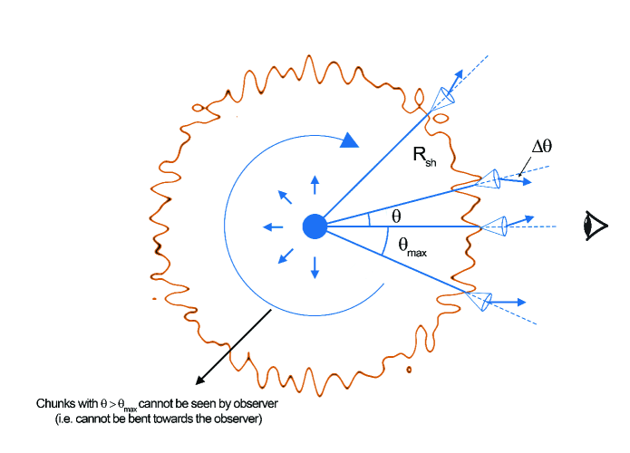
Figure 13: Our model for repeating FRBs: A plasma shell (e.g. an HII region) at a distance $R_{\rm sh.}$ from the QN explosion acts as a refractor. In this simple geometry, the FRBs beams from the QN chunks are each bent by an angle $\Delta\theta\leq\theta_{\rm max.}$, in random direction, by the refracting plasma. Repeating FRBs occur when multiple beams are bent towards the observer by any inhomogeneities in the shell (see Appendix G).

We argue that these are “twinkling FRBs” due to refractive ionized plasma (e.g. HII regions) in the vicinity of the SN explosion. Let us assume that the QN is surrounded by a thin shell of ionized plasma (e.g. an HII region) at radius $R_{\rm sh.}$. The shell has a refraction index $n_{\rm sh.}=\sqrt{1-\nu_{\rm sh.,p}/\nu}$ with $\nu_{\rm sh.,p}$ the shell’s plasma frequency. We assume that each emission beam (with initial beam-width $\sim 1/\Gamma_{\rm QN}$) from the $N_{\rm c}$ QN chunks is bent by an angle $\Delta\theta_{\rm sh.}\leq\theta_{\rm max.}$ in a random direction. Here $\theta_{\rm max.}$ is the maximum bending angle (see Figure 13). Thus the probability of seeing any one beam (i.e. a beam scattered towards the observer) is

$$P_{1}=\frac{\pi(1/\Gamma_{\rm QN}^{2})}{\pi\theta_{\rm max.}^{2}}\ .$$ (1)

As can be seen from Figure 13, beams in the $\theta>\theta_{\rm max.}$ quadrant cannot be seen by the observer. For $\theta<\theta_{\rm max.}$ the number of beams that are scattered randomly is

$$N_{\rm scat.}=\frac{\pi\theta_{\rm max.}^{2}}{4\pi}N_{\rm c}\ .$$ (2)

The above implies that the total probability of seeing one beam scattered towards the observer is

$$P_{\rm T,1}=P_{1}\times N_{\rm scat.}=\frac{N_{\rm c}}{4\Gamma_{\rm QN}^{2}}\ .$$ (3)

In our model thus, a repeating FRB occurs only if $P_{\rm T,1}\geq 1$ or when

$$N_{\rm c}>4\Gamma_{\rm QN}^{2}=4\times 10^{7}\times\Gamma_{\rm QN,3.5}^{2}\ .$$ (4)

The implication of Eq. (4) above is that a typical chunk in a QN where a a repeating FRB occurs has a mass $m_{\rm c,RFRB}<m_{\rm c,FRB}/40$; for our fiducial values $N_{\rm c}=10^{6}$. Since the FRB luminosity is linearly proportional to the chunk’s mass (see Eq. 72), this means that the luminosity of an RFRB is such that $L_{\rm RFRB}<L_{\rm FRB}/40$.

The maximum duration of the entire repeating episode is the time delay between $\theta=0$ and $\theta_{\rm max.}$, or

$$\Delta t_{\rm max}=\frac{R_{\rm sh.}(1-\cos{\theta_{\rm max.}})}{c}\sim 32.6\ {\rm years}\times R_{\rm sh.,1}(1-\cos{\theta_{\rm max.}})\ .$$ (5)

with $R_{\rm sh.,1}=R_{\rm sh.}/10\ {\rm pc}$. We can estimate a minimum repeating timescale by using the typical separation in angle between chunks of $\theta_{\rm sep.}=(4/N_{\rm c}^{1/2})$ which gives

$$\Delta t_{\rm min}=\frac{R_{\rm sh.}(1-\cos{\theta_{\rm sep.}})}{c}\simeq\frac{R_{\rm sh.}\theta_{\rm sep.}^{2}}{2c}\sim 0.23\ {\rm hours}\times\frac{R_{\rm sh.,1}}{N_{\rm c,7}}\ .$$ (6)

Assuming the refraction process is Poissonian in nature (i.e. when $P_{\rm T,1}>1$) we can estimate the probability of detecting $k$ bursts during $\Delta t_{\rm max}$ as $P(k)=\frac{(P_{\rm T,1})^{k}e^{-P_{\rm T,1}}}{k!}$ which has a peak at $k\sim 5$ if $P_{\rm T,1}\sim 1$. To explain clustered events (like observed repeating FRBs) we must appeal to coherence inhomogeneities in the refracting shell capable of refracting adjacent beams towards the observer. Defining $\theta_{\rm coh.}$ as the angular scale of the coherence scale, to get $\sim 10$ FRBs within a time interval of a few times $\Delta t_{\rm min}$, the coherence angular scale must be a few times $\theta_{\rm sep.}$. The corresponding coherence scale is $R_{\rm sh.}\theta_{\rm coh.}=R_{\rm sh.}\times 6/\Gamma_{\rm QN}\sim 4000$ AU.

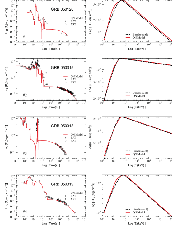
Figure 6: GRB simultaneous light-curve and spectrum fits: The light-curve (left panel) and spectrum (right panel) fits for each of the 48 LGRBs listed in Table LABEL:table:lcfits. For the light-curves, the BAT data is extrapolated to the XRT band and shown as black crosses. The XRT data is shown as open circles. The red line is the QN model. For the spectra, the red line is the QN model whereas the black dashed line is the best-fit Band function to the observed spectrum from Yonetoku et al. (2010).

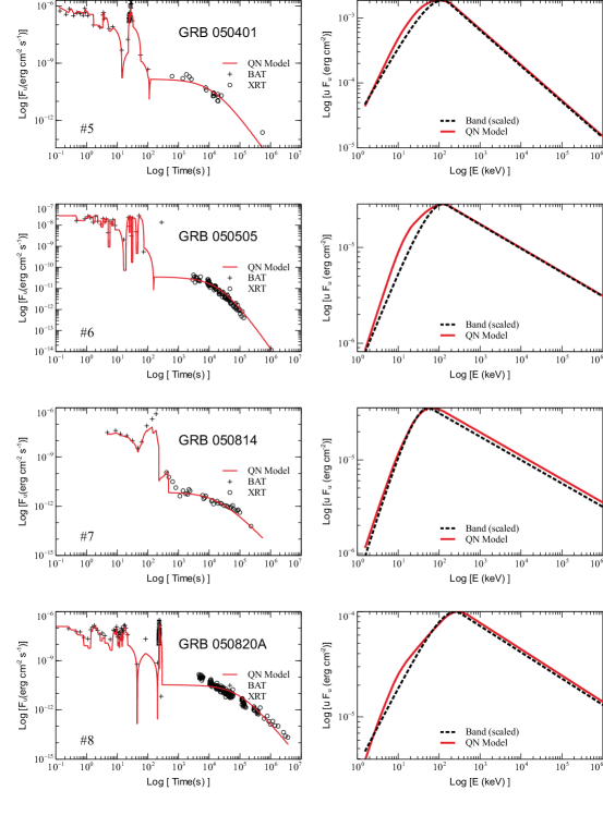
Figure 6 (Cont.):

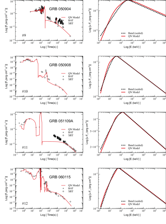
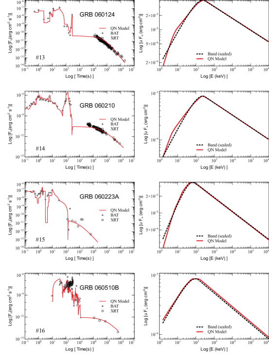
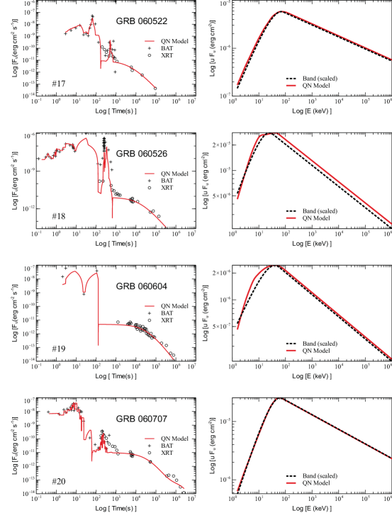
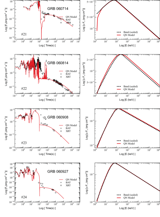
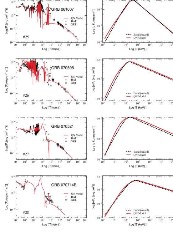
Figure 6 (Cont.):

Figure 6 (Cont.):

Figure 6 (Cont.):

Figure 6 (Cont.):

Figure 6 (Cont.):

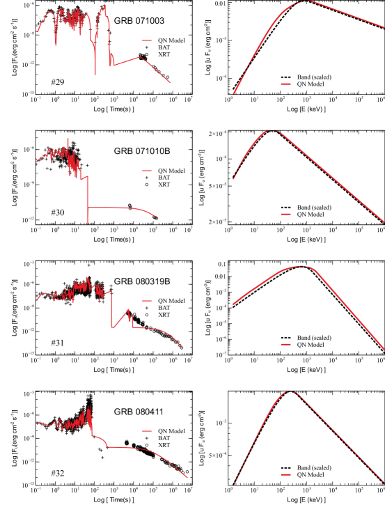
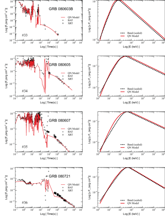
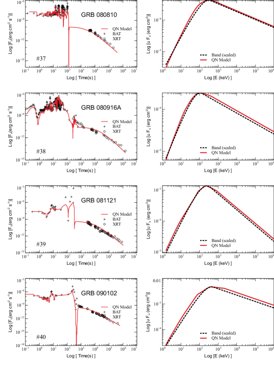
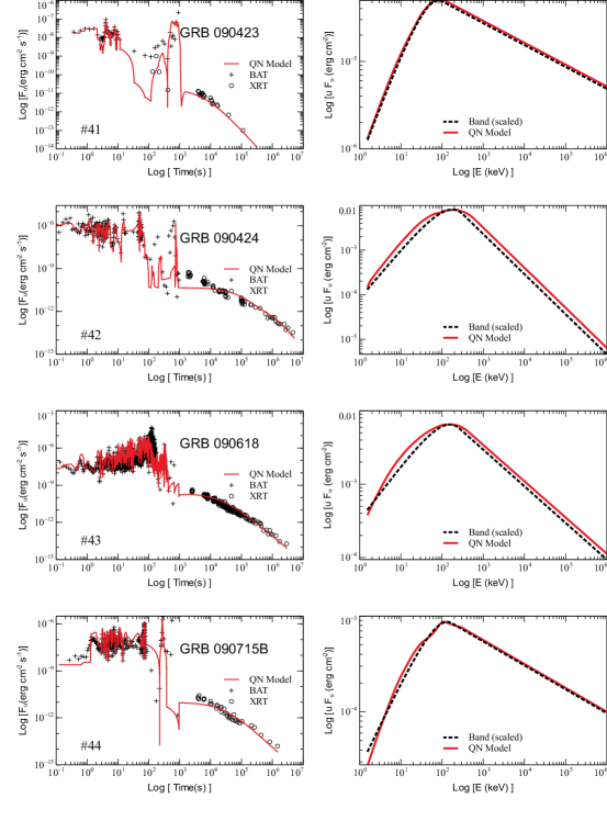
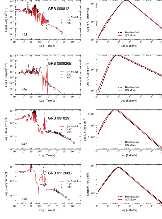
Figure 6 (Cont.):

Figure 6 (Cont.):

Figure 6 (Cont.):

Figure 6 (Cont.):

Figure 6 (Cont.):

Figure 7: Flares in our model: Top panel: Illustration of how flares are produced in our model. A simulated GRB with a single filament and four chunks at $\theta_{\rm c}=0.000,0.001,0.002,$ and $0.003$ rads. This panel demonstrates how the emission gets shifted to longer times and lower flux as $\theta_{\rm c}$ increases; the afterglow is the plateau for each $\theta_{\rm c}$. Here, $\theta_{\rm c}=0.000$ represents the primary chunk responsible for the prompt emission. To see a flare, the secondary chunk should be at a $\theta_{\rm c}$ large enough that it does not overlap with the primary chunk peak, but not so large that it is fainter than the afterglow (like the chunk at $\theta_{\rm c}=0.003$ rads). Bottom panel: The data for GRB 060707 is represented by the open circles with a flare at $\sim 10^{2.5}$ s. Using the simulation results from §  5.3.5 we show, in purple, the light-curve produced by a single, primary chunk at $\theta_{\rm P}=4\times 10^{-4}$ rad. The light-curve from a secondary chunk at $\theta_{\rm S}=2.7\times 10^{-3}$ rad is shown in purple (scaled by 40).

Figure 8: Model parameters: Distributions of parameters from simultaneous fits to light-curves and spectra of the 48 LGRBs listed in Table LABEL:table:lcfits. See §  5.3.4, Table 1 and Table LABEL:table:lcfits for definitions of parameters. We use Rice’s rule for binning.

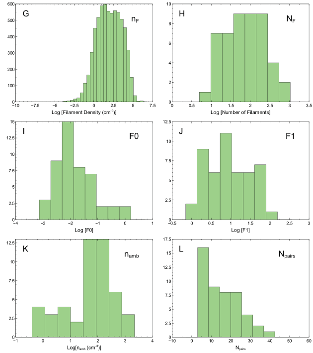
Figure 8 (Cont.):

Figure 9: Model timescales: Distribution of timescales from simultaneous fits to light-curves and spectra of the 48 selected LGRBs. Panel A: the distribution of $t_{\rm QN}=t_{\rm SpD}$ resulting from the $B_{\rm NS}$ distribution (see panel A of Figure 8). Panel B: the distributions of the minimum and maximum values of the thickness parameter $t_{\rm w}/t_{\Gamma}$. This shows the wide variation of filaments’ thickness within each GRB and from one GRB to another. Panel C: the distribution of durations of the 48 fit LGRBs compared to the $t_{90}$ of all GRBs (data from https://swift.gsfc.nasa.gov/archive/grb_table). The fit LGRBs have durations representative of the LGRB population.

Figure 15: PWN-SN shell (“the Wall”) column density: The relative column density $\sum{n_{\rm F}\Delta R_{\rm F}}$ normalized to the analytical value $n_{\rm Plat.}\times(R_{\rm w}/12$) (see §  3). Each column density (one per fit LGRB) is generated by adding up all the filaments along the line-of-sight for a single LGRB.

References

- Aab et al. (2014) Aab, A., et al. (The Pierre Auger Collaboration) 2014, Phys. Rev. D, 90, 122005
- Abbasi et al. (2012) Abbasi, R., Abdou, Y. Abu-Zayyad, T., et al. 2012, Nature 484, 351
- Abbott et al. (2017a) Abbott, B. P., et al. (LIGO Scientific Collaboration and Virgo Collaboration), 2017a, Phys. Rev. Lett., 119, 161101
- Abbott et al. (2017b) Abbott, B. P., Abbott, R., Abbott, T. D., et al. 2017b, ApJ, 848, L12
- Achterberg et al. (2001) Achterberg, A., Gallant, Y. A., Kirk, J. G., & Guthmann, A. W. 2001, MNRAS, 328, 393
- Achterberg & Wiersma (2007) Achterberg, A. & Wiersma, J. 2007, A&A, 475, 1
- Ai et al. (2018) Ai, S., Gao, H., Dai, Z-G et al. 2018, ApJ, 860, 57
- Akmal et al. (1998) Akmal, A., Pandharipande, V. R., & Ravenhall, D. G. 1998, Phys. Rev. C, 58, 1804
- Alford et al. (2007) Alford, M., Blaschke, D., Drago, A., et al. 2007, Nature, 445, 7
- Aloisio (2018) Aloisio, R. 2018, “The Physics of UHECRs: Spectra, Composition and the Transition Galactic-Extragalactic”, in Proceedings of 2016 International Conference on Ultra-High Energy Cosmic Rays (UHECR2016), 011008
- Amati et al. (2002) Amati L., Frontera F., Tavani M., et al. 2002, A&A, 390, 81
- Amati et al. (2006) Amati L., Della Valle M., Frontera F., et al. 2006, A&A, 463, 913
- Andersson et al. (1999) Andersson, N., Kokkotas, K., & Schutz, B. F. 1999, ApJ, 510, 846
- Andersson et al. (2000) Andersson, N., Jones, D. I., Kokkotas, K. D., & Stergioulas, N. 2000, ApJ, 534, L75
- Auger (1935) Auger, P. 1935, Nature, 135, 820
- Åström et al. (2004) Åström, J. A., et al. 2004, Phys. Rev. E, 70, 026104
- Bagoly et al. (2006) Bagoly, Z., et al. 2006, A&A, 453, 797
- Baiotti et al. (2013) Baiotti, L., Giacomazzo, B., & Rezzolla, L. 2008, Phys. Rev. D, 78, 084033
- Band et al. (1993) Band, D. L., et al. 1993, ApJ, 413, 281
- Band et al. (2004) Band D. L., et al. 2004, ApJ, 613, 484
- Barber et al. (2006) Barber et al. 2006, in “The Swift BAT Instrument: Performance and Results”, proceedings of the 36th COSPAR Scientific Assembly, 36, 1834
- Barkov & Pozanenko (2011) Barkov M. V., & Pozanenko A. S., 2011, MNRAS, 417, 2161
- Barraud et al. (2003) Barraud, C., et al. 2003, A&A, 440, 809
- Barthelmy et al. (2005) Barthelmy, S. D. et al. 2005, Nature, 483, 994 ,
- Basak & Rao (2015) Basak, R., & Rao, A. R. 2015, ApJ, 807, 34
- Batista et al. (2017) Batista, A. R., Shin, M.-S., Devriendt, J., Semikoz, D., & Sigl, G. 2017, Phys. Rev. D, 96, 023010
- Bauswein et al. (2010) Bauswein, A., Janka, H.T., & Oechslin, R. 2010, Phys. Rev. D, 82, 084043
- Beloborodov (2002) Beloborodov, A. M. 2002, ApJ, 565, 808
- Beloborodov (2010) Beloborodov A. M. 2010, MNRAS, 407, 1033
- Berezhiani et al. (2003) Berezhiani, Z., Bombaci, I., Drago, A., Frontera, F., & Lavagno, A. 2003, ApJ 586, 1250
- Berezinsky et al. (2006) Berezinsky, V., Gazizov, A., & Grigorieva, S. 2006, Phys. Rev. D, 74, 043005
- Berezinsky (2008) Berezinsky, V. 2008, Propagation and origin of ultra high-energy cosmic rays. Adv. Space Res.41, 2071
- Berger et al. (2007) Berger, E., Fox, D. B., Price, P. A., et al. 2007, ApJ, 664,1000
- Berger (2010) Berger E. 2010, ApJ, 722, 1946
- Berger (2014) Berger, E. 2014, ARA&A, 52, 43
- Bietenholz & Bartel (2017) Bietenholz, M. F. & Bartel, N. 2017, ApJ, 851, 124
- Blandford & McKee (1976) Blandford, R.D. & McKee, C.F. 1976, Phys. Fluids 1976, 19, 1130
- Bisnovatyi-Kogan (2006) Bisnovatyi-Kogan, G. S. 2006, Phys. Part. Nucl., 37, 647
- Blinnikov et al. (1984) Blinnikov, S. I., Novikov, I. D., Perevodchikova, T. V., & Polnarev, A. G. 1984, SvAL, 10, 177
- Blondin et al. (1998) Blondin, J. M., Wright, E. B., Borkowski, K. J., & Reynolds, S. P. 1998, ApJ, 500, 342
- Blondin et al. (2001) Blondin, J. M., Chevalier, R. A., & Frierson, D. M. 2001, ApJ, 563, 806
- Blondin & Chevalier (2017) Blondin, J. M. & Chevalier, R. A. 2017, ApJ, 845, 139
- Bloom et al. (1999) Bloom J. S., et al., 1999, Nature, 401, 453
- Bloom et al. (2002) Bloom, J. S., Kulkarni, S. R. & Djorgovski, S. G. 2002, AJ, 123, 1111
- Bodmer (1971) Bodmer, A. R. 1971, Phys. Rev. D, 4, 1601
- Bombaci, Parenti & Vidana (2004) Bombaci, I. Parenti, I. & Vidana, I. 2004, ApJ, 614, 314
- Bombaci et al. (2009) Bombaci, I., Logoteta, D., Panda, P. K., Providência, C., & Vidaña, I. 2009, Physics Letters B, 680, 448
- Bromberg et al. (2013) Bromberg O, Nakar E, Piran T, & Sari R. 2013, ApJ, 764, 179
- Brown & Wohletz (1995) Brown, W. K. & Wohletz 1995, K. H., Journal of Applied Physics, Vol. 78, 4, 2758
- Bucciantini et al. (2004) Bucciantini, N., Amato, E., Bandiera, R., Blondin, J. M., & Del Zanna, L. 2004, A&A, 423, 253
- Bucciantini et al. (2012) Bucciantini N., Metzger B. D., Thompson T. A., & Quataert E. 2012, MNRAS, 419, 1537
- Burlon (2008) Burlon, D., et al. 2008, ApJ, 685, L19
- Burrows et al. (2005) Burrows, D. N., Romano, P., Falcone, A., et al. 2005, Science, 309, 1833
- Butler et al. (2007) Butler N. R., Kocevski D., Bloom J. S., Curtis J. L., 2007, ApJ, 671, 656
- Bykov et al. (2012) Bykov A., Gehrels N., Krawczynski H., Lemoine M., Pelletier G., & Pohl M. 2012, Space Sci. Rev., 173, 309
- Camilo & Rasio (2005) Camilo, F., & Rasio, F. A. 2005, Binary Radio Pulsars, 328, 147
- Campana et al. (2006) Campana S, et al. 2006, A&A, 454, 113
- Cappellaro et al. (2015) Cappellaro, E., Botticella, M. T., Pignata, G., et al. 2015, A&A, 584, A62
- Cavallo & Rees (1978) Cavallo, G., & Rees, M. J. 1978, MNRAS, 183, 359
- Champion et al. (2016) Champion, D. J., Petroff, E., Kramer, M., et al. 2016, MNRAS, 460, L30
- Chen & Beloborodov (2007) Chen, W. X., & Beloborodov, A. M. 2007, ApJ, 657, 383
- Cheng & Dai (1996) Cheng, K. S., & Dai, Z. G. 1996, Phys. Rev. Lett., 77, 1210
- Chevalier (1977) Chevalier, R. A. 1977, ARA&A, 15, 175
- Chevalier & Klein (1978) Chevalier, R. A., & Klein, R. I. 1978, ApJ, 219, 994
- Chevalier (1982) Chevalier, R. A. 1982, ApJ, 258, 790
- Chevalier (1984) Chevalier, R. A. 1984, ApJ, 280, 797
- Chevalier (2005) Chevalier, R. A. 2005, ApJ, 619, 839
- CHIME/FRB Collaboration (2019) CHIME/FRB Collaboration, Amiri, M., Bandura, K., et al. 2019, Nature, 566, 235
- Chincarini et al. (2010) Chincarini, G., Mao, J., Margutti, R., et al. 2010, MNRAS, 406, 2113
- Christodoulou & Ruffini (1971) Christodoulou, D., & Ruffini, R., 1971,Phys. Rev. D, 4, 3552
- Ciolfi et al. (2017) Ciolfi, R. Kastaun, W. Giacomazzo, B. et al. 2017, Phys. Rev. D, 95, 063016
- Collazzi et al. (2012) Collazzi, A. C., Schaefer, B. E., Goldstein, A., & Preece, R. D. 2012, ApJ, 747, 39
- Connor et al. (2016) Connor, L., Sievers, J., Pen, U.-L., 2016, MNRAS, 458, L19
- Conselice et al. (2005) Conselice, C. J., Blackburne, J. A., & Papovich, C. 2005, ApJ, 620, 564
- Cordes & Wasserman (2016) Cordes J. M., & Wasserman I., 2016, MNRAS, 457, 232
- Cordes & Chatterjee (2019) Cordes, J. M. & Chatterjee, S., 2019 [arXiv:1906.05878]
- Costa et al. (1997) Costa, E., Frontera, F., Heise, J., et al. 1997, Nature, 387, 783
- Costa & Frontera (2011) Costa, E. & Frontera, F. 2011, Riv. Nuovo Cim., 34, 585
- Covino et al. (2005) Covino, S., et al. 2005, GRB Coordinates Network, 3665, 1
- Covino et al. (2010) Covino, S., et al. 2010, A&A, 521
- Dai et al. (1995) Dai, Z., Peng, Q., & Lu, T. 1995, ApJ, 440, 815
- Dai & Lu (1998) Dai, Z. G. & Lu T. 1998, Phys. Rev. Lett., 81, 4301
- Dai et al. (2011) Dai, S., Li, L., & Xu, R. 2011, Science China Physics, Mechanics, and Astronomy, 54, 1541
- Dai et al. (2016) Dai, Z. G., Wang J. S., Wu X. F., Huang Y. F., 2016, ApJ, 829, 27
- Dainotti et al. (2008) Dainotti, M. G., Cardone, V. F., & Capozziello, S. 2008, MNRAS, 391L, 79D
- Dainotti & Amati (2018) Dainotti, M. G., & Amati, L. 2018, PASP, 130, 051001
- Dainotti (2018) Dainotti, M. G., Del Vecchio, R., & Tarnopolski, M. 2018, Advances in Astronomy, 2018, 4969503
- Damour & Ruffini (1975) Damour, T., & Ruffini, R., 1975, Phys. Rev. Lett., 35, 463
- Dar & de Rújula (2004) Dar, A., & de Rújula, A. 2004, Phys. Rep., 405, 203
- Dar (2006) Dar, A. 2006, Chinese Journal of Astronomy and Astrophysics Supplement, 6, 301
- Dass & Soni (2012) Dass, N. D. H., & Soni, V. 2012, MNRAS, 425, 1558
- D’Avanzo et al. (2009) D’Avanzo P., et al., 2009, A&A, 498, 711
- D’Avanzo et al. (2014) D’Avanzo, P., Salvaterra, R. & Bernardini, M. G., MNRAS, 2014, 442, 2342
- D’Avanzo (2015) D’Avanzo P., 2015, Journal of High Energy Astroph., 7, 73
- Demorest al. (2010) Demorest, P. B., et al. 2010, Nature, 467, 1081
- Deutsch (1955) Deutsch, A. J. 1955, AnAp, 18, 1
- Di Matteo et al. (2002) Di Matteo, T., Perna, R., & Narayan, R. 2002, ApJ, 579, 706
- Drago, Lavagno, & Pagliara (2004) Drago, A. Lavagno, A., & Pagliara, G. 2004, Phys. Rev. D, 69, 057505
- Drago & Pagliara (2015a) Drago, A., & Pagliara, G. 2015a, Phys. Rev. C, 92, 045801
- Drago & Pagliara (2015b) Drago, A., & Pagliara, G. 2015b, European Physical Journal A, 52, 41
- Drago et al. (2016) Drago, A., Lavagno, A., Metzger, B. D., & Pagliara, G. 2016, Phys. Rev. D, 93, 103001
- Duffell & Kasen (2017) Duffell, P. C., & Kasen, D. 2017, ApJ, 842, 18
- Duncan & Thompson (1992) Duncan R. C., & Thompson C., 1992, ApJ, 392, L9
- Dvornikov (2016a) Dvornikov, M. 2016a, Physics Letters B, 760, 406
- Dvornikov (2016b) Dvornikov, M. 2016b, Nuclear Physics B, 913, 79
- Eichler et al. (1989) Eichler, D., Livio, M., Piran, T., & Schramm, D. N. 1989, Nature 340, 126
- Elliott et al. (2013) Elliott, J., Krühler, T., Greiner, J., et al. 2013, A&A, 556, A23
- Evans et al. (2010) Evans, P. A., Willingale, R., Osborne, J. P., et al. 2010, A&A, 519, A102
- Falcone et al. (2007) Falcone, A. D., Morris, D., Racusin, J., et al. 2007, ApJ, 671, 1921
- Faucher-Giguère & Kaspi (2006) Faucher-Giguère, C.-A., & Kaspi, V. M. 2006, ApJ, 643, 332
- Fenimore & Ramirez-Ruiz (2000) Fenimore E. E., & Ramirez-Ruiz E., 2000, preprint (astro-ph/0004176)
- Fermi, (1949) Fermi, E. 1949, Phys. Rev., 75, 1169
- Filippenko (1997) Filippenko, A. V. 1997, ARA&A, 35, 309
- Firmani et al. (2006) Firmani C., Ghisellini G., Avila-Reese V., & Ghirlanda G., 2006, MNRAS, 370, 185
- Fishman & Meegan (1995) Fishman, G. J., & Meegan, C. A. 1995, ARA&A, 33, 415
- Fox&Roming (2007) Fox, D. B., & Roming, P. W. A. Phil. Trans. R. Soc. A 2007 365, 1293
- Frail, et al. (2001) Frail, D. A., Kulkarni, S. R., Sari, R., et al. 2001, ApJ, 562, L55
- Fried (1959) Fried, B. D. 1959, Physics of Fluids, 2, 337
- Fruchter et al. (2006) Fruchter, A. S., et al., 2006, Nature, 441, 463
- Fujibayashi et al. (2018) Fujibayashi, S. Kiuchi, K., Nishimura, N., Sekiguchi, & Y. Shibata, M. 2018, ApJ, 860, 64
- Furusawa et al. (2016a) Furusawa, S., Sanada, T., & Yamada, S. 2016a, Phys. Rev. D, 93, 4, 043018
- Furusawa et al. (2016b) Furusawa, S., Sanada, T., & Yamada, S. 2016b, Phys. Rev. D, 93, 4, 043019
- Fynbo et al. (2006) Fynbo, J. P. U., et al. 2006, Nature, 444, 1047
- Gajjar et al. (2018) Gajjar, V., Siemion, A. P. V., Price, D. C., et al. 2018, ApJ, 863, 2
- Galama et al. (1998) Galama, T. J., Vreeswijk, P. M., van Paradijs, J., et al. 1998, Nature, 395, 670
- Gallant & Achterberg (1999) Gallant, Y. A. & Achterberg, A. 1999, MNRAS, 305, L06
- Gao et al. (2016) Gao, H., Zhang, B. & Lü, H.-J. 2016, Phys. Rev. D, 93, 4, 044065
- Gehrels et al. (2005) Gehrels N., et al., 2005, Nature, 437, 851
- Gehrels et al. (2009) Gehrels, N. Ramirez-Ruiz & E. Fox, D. B. 2009, ARA&A, 47, 567
- Geng & Huang (2015) Geng, J. J., & Huang, Y. F. 2015, ApJ, 809, 24
- Ghirlanda et al. (2003) Ghirlanda G., Celotti A., & Ghisellini G., 2003, A&A, 406, 879
- Ghirlanda et al. (2004) Ghirlanda G., Ghisellini G., & Lazzati D., 2004, ApJ, 616, 331
- Ghirlanda et al. (2009) Ghirlanda, G., Nava, L., Ghisellini, G., Celotti, A., & Firmani, C. 2009, A&A, 496, 585
- Ghirlanda et al. (2011) Ghirlanda, G., Ghisellini, G., & Nava, L. 2011, MNRAS, 418, L109
- Giacomazzo & Perna (2013) Giacomazzo, B. & Perna, R. 2013, ApJ, 771, L26
- Giannios (2006) Giannios, D. 2006, A&A, 455, L5
- Goldreich & Keeley (1971) Goldreich, P. & Keeley, D. A., 1971, ApJ, 170, 463
- Goodman (1986) Goodman J., 1986, ApJ, 308, L47
- Gompertz, O’Brien & Wynn (2014) Gompertz, B. P., O’Brien, P. T. & Wynn, G. A. 2014, MNRAS, 438, 240
- Granot (2005) Granot, J. 2005, ApJ, 631, 1022
- Grupe et al. (2009) Grupe, D., Burrows, D., Wang, X.-Y., et al. 2009, American Institute of Physics Conference Series, 1133, 163
- Gu et al. (2006) Gu, W. M., Liu, T., & Lu, J. F. 2006, ApJ, 643, L87
- Gu et al. (2016) Gu, W. M., Gong, Y. Z., Liu, T., Ma, R., & Wang, J. 2016, ApJ, 823, L28
- Hebeler et al. (2013) Hebeler, K., Lattimer, J. M., Pethick, C. J., & Schwenk, A., 2013, ApJ, 773, 11
- Heger et al. (2003) Heger, A., Fryer, C. L., Woosley, S. E., Langer, N., & Hartmann, D. H. 2003, ApJ, 591, 288
- Heinz&Begelman (1999) Heinz, S., & Begelman, M. 1999, ApJ, 527, L35
- Heise et al. (2001) Heise, J., t Zand, J. I., Kippen, R. M., & Woods, P. M. 2001, Gamma-Ray Bursts in the Afterglow Era: Proceedings of the International Workshop Held in Rome, Italy, 17-20 October 2000, ESO ASTROPHYSICS SYMPOSIA. ISBN 3-540-42771-6. Edited by E. Costa, F. Frontera, and J. Hjorth. Springer-Verlag, p. 16
- Herzog & Röpke (2011) Herzog, M., & Röpke, F. K. 2011, Phys. Rev. D, 84, 083002
- Heussaff et al. (2013) Heussaff, V., Atteia, J.-L., & Zolnierowski, Y. 2013, A&A, 557, A100
- Hjorth et al. (2003) Hjorth J., Sollerman, J., & Møller, P., et al. 2003, Nature, 423, 847
- Hjorth & Bloom (2012) Hjorth, J., & Bloom, J. S. 2012, Chapter 9 in “Gamma-Ray Bursts”, CambridgeAstrophysics Series 51, eds. C. Kouveliotou, R. A. M. J. Wijers and S. Woosley, Cambridge University Press (Cambridge), p. 169
- Horesh et al. (2016) Horesh, A., Hotokezaka, K., Piran, T., Nakar, E. & Hancock, P. 2016, ApJ, 819, L22
- Horvath & Benvenuto (1988) Horvath, J. E., & Benvenuto, O. G. 1988, Phys. Lett. B, 213, 516
- Horváth (1998) Horváth, I. 1998, ApJ, 508, 757
- Hotokezaka et al. (2011) Hotokezaka, K., Kyutoku, K., Okawa, H., Shibata, M., & Kiuchi, K. 2011, Phys. Rev. D, 83, 124008
- Hotokezaka et al. (2013) Hotokezaka, K., Kiuchi, K., Kyutoku, K., et al. 2013, Phys. Rev. D, 87, 024001
- Hou et al. (2018) Hou, S.-J., Liu, T., Xu, R.-X. et al. 2018, ApJ, 854, 104
- Iida & Sato (1998) Iida, K., & Sato, K. 1998, Phys. Rev. C, 58, 2538
- Ikeda et al. (2007) Ikeda, M., Takeda, A., Fukuda, Y., et al. 2007, ApJ, 669, 519.
- Itoh (1970) Itoh, N. 1970, Prog. Theor. Phys., 44, 291
- Iwamoto et al. (1998) Iwamoto, K., et al. 1998, Nature, 395, 672
- Iwazaki (2005) Iwazaki, A. 2005, Phys. Rev. D, 72, 114003
- Iyyani (2018) Iyyani, S. 2018, Journal of Astrophysics and Astronomy, 39, 75
- Jaikumar et al. (2004) Jaikumar, P., Balaji, K. R., & Gale, C. 2004, Phys. Rev. C, 69, 055804
- Jaikumar et al. (2007) Jaikumar, P., Meyer, B. S., Otsuki, K, & Ouyed, R. 2007, A&A, 471, 227
- Janiuk et al. (2007) Janiuk, A., Yuan, Y., Perna, R., & Di Matteo, T. 2007, ApJ, 664, 1011
- Jun et al. (1995) Jun, B.-I., Norman, M. L., & Stone, J. M. 1995, ApJ, 453, 332
- Jun (1998) Jun, B.-I. 1998, ApJ, 499, 282
- Kasen et al. (2013) Kasen, D., Badnell, N. R., & Barnes, J. 2013, ApJ, 774, 25
- Kashiyama et al. (2013) Kashiyama, K., Ioka, K., & Mészáros, P. 2013, ApJ, 776, L39
- Kato (2007) Kato, T. 2007, ApJ, 668, 974
- Katz (2014) Katz, J. I. 2014, Phys. Rev. D, 89, 103009
- Katz (2016a) Katz, J. I. 2016a, Modern Physics Letters A, 31, 1630013
- Katz (2016b) Katz J. I., 2016b, ApJ, 826, 226
- Keränen et al. (2005) Keränen, P., Ouyed, R., & Jaikumar, P. 2005, ApJ, 618, 485
- King et al. (2005) King, A., O’Brien, P. T., Goad, M. R., et al. 2005, ApJ, 630, L113
- Klebesadel et al. (1973) Klebesadel, R. W., Strong, I. B., & Olson, R. A. 1973, ApJ, 182, L85
- Kobayashi et al. (1997) Kobayashi, S., Piran, T., & Sari, R. 1997, ApJ, 490, 92
- Korobkin et al. (2012) Korobkin, O., Rosswog, S., Arcones, A., & Winteler, C. 2012, MNRAS, 426, 1940
- Kostka et al. (2014a) Kostka, M., Koning, N., Leahy, D., Ouyed, R., & Steffen, W. 2014a, Revista Mexicana de Astronomía y Astrofísica, 50, 167
- Kostka et al. (2014b) Kostka, M., Koning, K., Shand, Z. Ouyed, R., & Jaikumar, P. 2014b, A&A 568, A97
- Kostka et al. (2014c) Kostka, M., Koning, K., Shand, Z. Ouyed, R., & Jaikumar, P. 2014c [arXiv:1402.3824]
- Kostka (2014) Kostka, M. 2014, “Investigating astrophysical r-process sites: code (r-Java 2.0) and model (dual-shock quark nova) development”, Thesis (Ph.D.)–University of Calgary (Canada), 2014 [http://dx.doi.org/10.11575/PRISM/26628]
- Kotera (2011) Kotera, K. 2011, Phys. Rev. D, 84, 023002
- Kouveliotou et al. (1993) Kouveliotou, C., Meegan, C. A., Fishman, G. J., et al. 1993, ApJ, 413, L101
- Kulkarni et al. (2014) Kulkarni, S. R., Ofek, E. O., Neill, J. D., Zheng, Z., & Juric, M. 2014, ApJ, 797, 70
- Kulkarni (2018) Kulkarni, S. R. 2018, Nature Astronomy, 2, 832
- Kumar & Panaitescu (2000) Kumar P, & Panaitescu A, 2000, ApJ, 541, L51
- La Parola et al. (2006) La Parola V, et al. 2006, A&A, 454, 753
- Landau & Lifschitz (1959) Landau, L. D., & Lifschitz, E. M. 1959, Fluid Mechanics, Oxford: Pergamon Press
- Lang (1999) Lang, K. R. 1999, Astrophysical formulae, Third edition (New York: Springer)
- Laming (2014) Laming, J. M. 2014, Nature, 506, 298
- Lazzati (2005) Lazzati, D. 2005, MNRAS, 357, 722
- Leahy & Ouyed (2007) Leahy, D., & Ouyed, R. 2007 [arXiv:0710.2114]
- Leahy & Ouyed (2008) Leahy, D., & Ouyed, R. 2008, MNRAS, 387, 1193
- Leahy & Ouyed (2009) Leahy, D., & Ouyed, R. 2009, Advances in Astronomy, 2009, 306821
- Lee et al. (2000) Lee, H. K., Wijers, R. A. M. J., & Brown, G. E. 2000, PhR, 325, 83
- Lei et al. (2009) Lei, W. H., Wang, D. X., Zhang, L., et al. 2009, ApJ, 700, 1970
- Lei et al. (2013a) Lei, W. H., Zhang, B., & Liang, E. W. 2013a, ApJ, 756, 125
- Lei et al. (2013b) Lei, W. H., Zhang, B., Wu, X.-F. & Liang, E. W. 2013b, ApJ, 849, 47
- Lemoine & Pelletier (2010) Lemoine M. & Pelletier G., 2010, MNRAS, 402, 321
- Letaw et al. (1983) Letaw, J. R., Silberberg, R. & Tsao, C. H. 1983, ApJ, 51, 271
- Levesque et al. (2010) Levesque E. M., Kewley L. J., Graham J. F., & Fruchter A. S., 2010, ApJ, 712, L26
- Li (2000) Li, L. X. 2000, Phys. Rev. D, 61, 084016
- Li, et al. (2016) Li, A., Zhang, B., Zhang, N.-B. et al. 2016, Phys. Rev. D, 94, 083010
- Li (2007) Li, L., 2007, MNRAS, 379, 55
- Li et al. (2018a) Li, L., Wu, X.-F., Lei, W.-H., et al. 2018a, ApJS, 236, 26
- Li et al. (2018b) Li., L. B., Huang, Y. F., Geng, J. J., & Li, B. 2018b, \raa, 18, 61
- Li (2019) Li, L. 2019a, ApJS, 242, 16
- Li et al. (2019) Li, L., Geng, J.-J., Meng, Y.-Z. et al. 2019b [arXiv:1901.04925]
- Li-Xin & Paczyński (1998) Li-Xin, L., & Paczyński, B. 1998, ApJ, 507, L59
- Liang & Zhang (2005) Liang E., & Zhang B., 2005, ApJ, 633, 611
- LIGO Scientific Collaboration and Aasi et al. (2015) LIGO Scientific Collaboration and Aasi, J., Abbott, B. P., Abbott, R., et al. 2015, Class. Quant. Grav., 32, 7, 074001
- Linsley (1963) Linsley, J. 1963, Phys. Rev. Lett., 10, 146
- Liu et al. (2015) Liu, T., Hou, S. J., Xue, L., & Gu, W. M. 2015, ApJS, 218, 12
- Logoteta et al. (2012) Logoteta, D., Providencia, C., Vidana, I., & Bombaci, I. 2012, Phys. Rev. C, 85, 055807
- Lorimer et al. (2007) Lorimer, D. R., Bailes, M., McLaughlin, M. A., Narkevic, D. J., & Crawford, F. 2007, Science, 318, 777
- Lorimer et al. (2018) Lorimer, D. R. 2018, Nature Astronomy, 2, 860
- Lu et al. (2004) Lu, T., Huang, Y. F., Dai, Z. G. & Wei, D. M. 2004, in Cosmic Gamma-Ray Sources (eds. K. S. Cheng & G. E. Romero), Kluwer Academic Publishers, p 225
- Lü et al. (2015) Lü, H.-J., Zhang, B., Lei, W.-H., Li, Y., & Lasky, P. D. 2015, ApJ, 805, 89
- Lugones et al. (1994) Lugones, G. Benvenuto, O., & Vucetich, H. 1994, Phys. Rev. D, 50, 6100
- MacFadyen & Woosley (1999) MacFadyen, A. I., & Woosley, S. E. 1999, ApJ, 524, 262
- Manchester & Taylor (1977) Manchester, R. N., & Taylor, J. H. 1977, Pulsars, Freeman, San Francisco
- Margalit & Metzger (2018) Margalit B., Metzger B. D., 2018, ApJ, 868, L4
- Marranghello et al. (2010) Marranghello, G. F., Araujo, J. C. N., & Miranda, O. D. 2010, Astronomy and Relativistic Astrophysics. New Phenomena and New States of Matter in the Universe, 99
- Mazets et al. (1981) Mazets, E.P., et al. 1981, Ap&SS, 80, 3
- Meech et al. (2017) Meech, K. J., Weryk, R., Micheli, M., et al. 2017, Nature, 552, 378
- Medvedev & Loeb (1999) Medvedev, M. V., & Loeb, A 1999, ApJ, 526, 697
- Meegan et al. (1992) Meegan, C. A., et al., 1992, Nature, 355, 143
- Mellinger et al. (2017) Mellinger, R., Weber, F., Spinella, W., Contrera, G., & Orsaria, Milva 2017, Universe, 3, 5
- Mésźaros & Rees (1992) Mésźaros, P., & Rees, M. J. 1992, MNRAS, 258, 41P
- Mészáros & Rees (1997) Mészáros, P., & Rees, M. J. 1997, ApJ, 476, 232
- Mészáros (2002) Mészáros, P. 2002, ARA&A, 40, 137
- Mészáros (2006) Mészáros, P. 2006, Rep. Prog. Phys. 69, 2259
- Metzger et al. (2008) Metzger, B. D., Quataert, E., & Thompson T. A., 2008, MNRAS, 385, 1455
- Metzger et al. (2010a) Metzger B. D., Arcones A., Quataert E., & Martínez-Pinedo G., 2010a, MNRAS, 402, 2771
- Metzger et al. (2010b) Metzger, B. D., Martínez-Pinedo, G., & Darbha, S., et al. 2010b, MNRAS, 406, 2650
- Metzger & Bower (2014) Metzger, B. D., & Bower, G. C. 2014, MNRAS, 437, 1821
- Metzger et al. (2017) Metzger B. D., Berger E., Margalit B., 2017, ApJ, 841, 14
- Michilli et al. (2018) Michilli, D., Seymour, A., Hessels, J. W. T., et al. 2018, Nature, 553, 182
- Mintz et al. (2010) Mintz, B., Fraga, E, Pagliara, G., & Schaffner-Bielich, J. 2010, Phys. Rev. D, 81, 123012
- Modjaz et al. (2016) Modjaz, M., Liu, Y. Q., Bianco, F. B., & Graur, O. 2016, ApJ, 832, 108
- Montez & Zarka (2014) Montez, K., & Zarka, P. 2014, A&A, 569, A86
- Mukherjee et al. (1998) Mukherjee, S., Feigelson, E.D., Babu, G.J., Murtagh, F., Fraley, C., & Raftery, A. 1998, ApJ, 508, 314
- Murase & Takami (2009) Murase, K., & Takami, H. 2009, ApJ, 690, L14
- Nakar & Piran (2005) Nakar, E., & Piran, T. 2005, MNRAS, 360, L73
- Nakar (2007) Nakar, E. 2007, Phys. Rep., 442, 166
- Nakar & Piran (2011) Nakar, E. & Piran, T. 2011, Nature, 478, 82
- Narayan, Paczynski & Piran (1992) Narayan, R., Paczyński, B., & Piran, T. 1992, ApJ, 395, L83
- Nishikawa et al. (2009) Nishikawa K.-I., Niemiec J., Hardee P. E., et al. 2009, ApJ, 698, L10
- Niebergal et al. (2010) Niebergal, B., Ouyed, R., & Jaikumar, P. 2010, Phys. Rev. C, 82, 062801
- Niebergal (2011) Niebergal, B., 2011, “Hadronic-to-Quark-Matter Phase Transition: Astrophysical Implications”, Thesis (Ph.D.)–University of Calgary (Canada), 2011.; Publication Number: AAT NR81856; ISBN: 9780494818565
- Niino et al. (2012) Niino, Y., Hashimoto, T., Aoki, K., et al. 2012, PASJ, 64, 115
- Nodvick & Saxon (1954) Nodvick, J. S., & Saxon, D. 1954, Phys. Rev. 96
- Nomoto et al. (2006) Nomoto, K., Tominaga, N., Tanaka, M., et al. 2006, Il Nuovo Cimento, 121, 1207
- Norris et al. (1984) Norris, J. P., Cline, T. L., Desai, U. D., & Teegarden, B. J. 1984, Nature, 308, 434
- Norris et al. (2000) Norris, J. P., Marani, G. F., & Bonnell, J. T. 2000, ApJ, 534, 248
- Norris & Bonnell (2006) Norris, J. P., & Bonnell, J. T. 2006, ApJ, 643, 266
- Norris, Gehrels & Scargle (2010) Norris J. P., Gehrels N., & Scargle J. D., 2010, ApJ, 717, 411
- Nousek et al. (2006) Nousek, J. A., Kouveliotou, C., Grupe, D., et al. 2006, ApJ, 642, 389
- Novokhatski (2012) Novokhatski, A. 2012, SLAC-PUB-14893
- O’Brien et al. (2006) O’Brien, P.T. et al. 2006, ApJ, 647, 1213
- Olesen & Madsen (1994) Olesen, M. L., & Madsen, J. 1994, Phys. Rev. D, 49, 2698
- Olinto (1987) Olinto, A. V. 1987, Physics Letters B 192, 71
- Ouyed, A. et al. (2014) Ouyed, A., Ouyed, R., Leahy, D., & Jaikumar, P. 2014, Rev. Mexicana Astron. Astrofis., 50, 77
- Ouyed, A. et al. (2015a) Ouyed, A., Ouyed, R., & Leahy, D. 2015a, Nuclear Physics A, 941, 241
- Ouyed, A. et al. (2015b) Ouyed, A., Welbanks, L., Koning, N., & Ouyed, R. 2015b, “The Burn-UD code for the numerical simulations of the Hadronic-to-Quark-Matter phase transition”, in Proceedings of the Compact Stars in the QCD Phase Diagram IV (CSQCD IV), September 26 - 30, 2014, Prerow, Germany, eds. Tobias Fischer and David Blaschke, http://www.slac.stanford.edu/econf/C140926/ [arXiv:1504.03590]
- Ouyed, A. et al. (2018a) Ouyed, A., Ouyed, R., & Jaikumar, P. 2018a, Physics Letters B, 777, 184
- Ouyed, A. et al. (2018b) Ouyed, A., Ouyed, R., & Jaikumar, P. 2018b, Universe, 4, 51
- Ouyed, A. (2018) Ouyed, A. 2018, “The Neutrino Sector in Hadron-Quark Combustion: Physical and Astrophysical Implications ”, Thesis (Ph.D.)–University of Calgary (Canada), 2018 [http://dx.doi.org/10.11575/PRISM/27841]
- Ouyed, A. et al. (2019) Ouyed, A., Ouyed, R., & Jaikumar, P. 2019, “The Structure of the Hadron-Quark Reaction Zone”, in Proceedings of the Compact Stars in the QCD Phase Diagram VII (CSQCD VII), June 11 - 15, 2018, NY, NY. Universe, 5(6), 136, eds. Vivian de la Incera, Efrain Ferrer, James Lattimer and David Blaschke [arXiv:1906.08404]
- Ouyed, R. et al. (2002) Ouyed, R., Dey, J., & Dey, M. 2002, A&A, 390, L39
- Ouyed, R. & Sannino (2002) Ouyed, R., & Sannino F. 2002, A&A 387, 725
- Ouyed, R. et al. (2004) Ouyed, R., Elgarøy, Ø., Dahle, H., & Keränen, P. 2004, A&A, 420, 1025
- Ouyed, R. et al. (2005) Ouyed, R., Rapp, R., & Vogt, C., 2005, ApJ, 632, 1001
- Ouyed, R. et al. (2006) Ouyed, R., Niebergal, B., Dobler, W., & Leahy, D. 2006, ApJ, 653, 558
- Ouyed, R. et al. (2007a) Ouyed, R., Leahy, D., & Niebergal, B. 2007a, A&A, 473, 357
- Ouyed, R. et al. (2007b) Ouyed, R., Leahy, D., & Niebergal, B. 2007b, A&A, 475, 63
- Ouyed, R. & Leahy (2009) Ouyed, R., & Leahy, D. 2009, ApJ, 696, 562
- Ouyed, R. et al. (2009a) Ouyed, R., Leahy, D., & Jaikumar, P. 2009a, “Predictions for signatures of the quark-nova in superluminous supernovae” in Proceedings of the “Compact stars in the QCD phase diagram II (CSQCD II)”, May 20-24, 2009, KIAA at Peking University, Beijing- P. R. China, eds. R. Ouyed & R. Xu, http://www.slac.stanford.edu/econf/C0905202/ [arXiv:0911.5424]
- Ouyed, R. et al. (2009b) Ouyed, R., Leahy, D., Staff, J., & Niebergal, B. 2009b, Advances in Astronomy, 2009, 463521
- Ouyed, R. et al. (2009c) Ouyed, R., Pudritz, R. E., & Jaikumar, P. 2009c, ApJ, 702, 1575
- Ouyed, R. et al. (2011a) Ouyed, R., Staff, J., & Jaikumar, P. 2011a, ApJ, 729, 60
- Ouyed, R. et al. (2011b) Ouyed, R., Staff, J., & Jaikumar, P. 2011b, ApJ, 743, 116
- Ouyed, R. et al. (2011c) Ouyed, R., Leahy, D., Ouyed, A., & Jaikumar, P. 2011c, Phys. Rev. Lett., 107, 151103
- Ouyed, R. et al. (2012) Ouyed, R., Kostka, M., Koning, N., Leahy, D. A., & Steffen, W. 2012, MNRAS, 423, 1652
- Ouyed, R. & Staff (2013) Ouyed, R., & Staff, J. 2013, \raa, 13, 435
- Ouyed, R. et al. (2013b) Ouyed, R., Koning, N., & Leahy, D. 2013a, \raa, 13, 1463
- Ouyed, R. et al. (2013a) Ouyed, R., Niebergal, B., & Jaikumar, P. 2013b, “Explosive Combustion of a Neutron Star into a Quark Star: the non-premixed scenario” in Proceedings of the Compact Stars in the QCD Phase Diagram III (CSQCD III), December 12-15, 2012, Guaruja, BRAZIL, eds. Laura Paulucci, Jorge E. Horvath, Marcelo Chiapparini, and Rodrigo P. Negreiros , http://www.slac.stanford.edu/econf/C121212/ [arXiv:1304.8048]
- Ouyed, R. et al. (2014) Ouyed, R., Koning, N., Leahy, D., Staff, J. E., & Cassidy, D. T. 2014, \raa, 14, 497-519
- Ouyed, R. et al. (2015a) Ouyed, R., Leahy, D., & Koning, N. 2015a, \raa, 15, 483
- Ouyed, R. et al. (2015b) Ouyed, R., Leahy, D., & Koning, N. 2015b, MNRAS, 454, 2353
- Ouyed, R. et al. (2015c) Ouyed, R., Leahy, D., & Koning, N. 2015c, ApJ, 809, 142
- Ouyed, R. et al. (2015d) Ouyed, R., Leahy, D., Koning, N., & Staff, J. 2015d, ApJ, 801, 64
- Ouyed, R. et al. (2016) Ouyed, R., Leahy, D., & Koning, N. 2016, ApJ, 818, 77
- Ouyed, R. et al. (2018a) Ouyed, R., Leahy, D., & Koning, N. 2018a, ApJ, 818, 77, “Quark-novae in binaries: Observational signatures and implications to astrophysics”, Proceedings of the Fourteenth Marcel Grossmann Meeting, 12-18 July 2015, Rome, Italy. Eds. M. Bianchi, R. T. Jansen and R. Ruffini (World Scientific Publishing Co. Pte. Ltd., ISBN #9789813226609), 1877
- Ouyed, R. et al. (2018b) Ouyed, R., Leahy, D., & Koning, N. 2018b, ApJ, 818, 77, “Quark-nova compact remnants: Observational signatures in astronomical data and implications to compact stars”, Proceedings of the Fourteenth Marcel Grossmann Meeting, 12-18 July 2015, Rome, Italy. Eds. M. Bianchi, R. T. Jansen and R. Ruffini (World Scientific Publishing Co. Pte. Ltd., ISBN #9789813226609), 3387
- O′Shaughnessy et al. (2008) O′Shaughnessy, R., Belczynski, K., & Kalogera, V. 2008, ApJ, 675, 566
- Pagliara et al. (2013) Pagliara, G., Herzog, M., & Röpke, F. K. 2013, Phys. Rev. D, 87, 103007
- Panaitescu (2008) Panaitescu, A., 2008, MNRAS, 383, 1143
- Paczyński (1971) Paczyński, B. 1971, ARA&A, 9, 183
- Paczyński (1986) Paczyński, B., 1986, ApJ, 308, L43
- Paczyński & Haensel (2005) Paczyński, B., & Haensel, P. 2005, MNRAS, 362, L4
- Peacock (1981) Peacock J. A., 1981, MNRAS, 196, 135
- Pe’er, Mészáros & Rees (2006) Pe’er A., Mészáros P., & Rees M. J., 2006, ApJ, 642, 995
- Pe’er (2012) Pe’er, A. 2012, ApJ, 752, L8.
- Pe’er (2015) Pe’er, A. 2015, Advances in Astronomy, 2015, 907321
- Peng et al. (2014) Peng, F.-K., Liang, E.-W., Wang, X.-Y., et al. 2014, ApJ, 795, 155
- Perez-Garcia et al. (2010) Perez-Garcia, M. A., Silk, J., & Stone, J. R. 2010, Phys. Rev. Lett., 105, 141101
- Perez-Garcia et al. (2013) Pérez-García, M. A, Daigne, F., & Silk, J. 2013, ApJ, 768, 145
- Petroff et al. (2016) Petroff, E., Barr, E. D., Jameson, A., et al. 2016, PASA, 33, e045
- Petroff et al. (2019) Petroff, E., Hessels, J. W. T. & Lorimer, D. R., 2019, Astronomy and Astrophysics Reviews, 27, 4
- Piran (1999) Piran, T. 1999, Phys. Rep, 314, 575
- Piran (2000) Piran, T. 2000, Phys. Rep., 333, 529
- Piran (2005) Piran, T. 2005, Rev. Mod. Phys. 76, 1143
- Piro et al. (2017) Piro, A. L., Giacomazzo., B. & Perna, R. 2017, ApJ, 844, 2, L19
- Piro et al. (2018) Piro, A. L., Troja, E., Zhang, B. et al. 2018, MNRAS, 483, 2, 1912
- Platts et al. (2018) Platts, E., Weltman, A., Walters, A., et al. 2018 [arXiv:1810.05836]
- Popham et al. (1999) Popham, R., Woosley, S. E., & Fryer, C. 1999, ApJ, 518, 356
- Popov et al. (2018) Popov, S. B., Postnov, K. A., & Pshirkov, M. S. 2018, Physics Uspekhi, 61, 965
- Porth et al. (2014) Porth, O., Komissarov, S. S., & Keppens, R. 2014, MNRAS, 443, 547
- Preece et al. (2000) Preece, R. D., Briggs, M. S., Mallozzi, R. S., et al., 2000, ApJS, 126, 19
- Preparata et al. (1998) Preparata, G., Ruffini, R., & Xue, S.-S., 1998, A&A, 338, L87
- Prochaska et al. (2009) Prochaska, J. X., Sheffer, Y., Perley, D. A., et al. 2009, ApJ, 691, L27
- Proga & Zhang (2006) Proga, D., & Zhang, B. 2006, MNRAS, 370, 61
- Ravi et al. (2016) Ravi, V., Shannon, R. M., Bailes, M., et al. 2016, Science, 354, 1249
- Ravi (2019) Ravi, V. 2019, Nature Astronomy, Jul., 405 [arXiv:1907.06619]
- Rees & Mészáros (1994) Rees M. J., & Mészáros, P., 1994, ApJ, 430, L93
- Reynolds & Chevalier (1984) Reynolds, S. P., & Chevalier, R. A. 1984, ApJ, 278, 630
- Reynolds et al. (2012) Reynolds, S. P., Gaensler, B. M., & Bocchino, F. 2012, Space Sci. Rev., 166, 231
- Rezzolla et al. (2010) Rezzolla, L., Baiotti, L., Giacomazzo, B., Link, D., & Font, J. A. 2010, Classical and Quantum Gravity, 27, 114105
- Rhoads (1997) Rhoads, J. E. 1997, ApJ, 487, L1
- Rhoads (1999) Rhoads, J. E. 1999, ApJ, 525, 737
- Řípa & Mészáros (2016) Řípa, J., & Mészáros, A. 2016, Ap&SS, 361, 370
- Rosswog & Liebendörfer (2003) Rosswog, S., & Liebendörfer, M. 2003, MNRAS, 342, 673
- Rosswog (2007) Rosswog S., 2007, MNRAS, 376, L48
- Rowlinson et al. (2013) Rowlinson A., O’Brien P. T., Metzger B. D., Tanvir N. R., & Levan A. J. 2013, MNRAS, 430, 1061
- Ruffert et al. (1996) Ruffert, M., Janka, H. -T. & Schaefer, G. 1996, A&A, 311, 532
- Ruffert & Janka (1999) Ruffert, M., & Janka, H.-T. 1999, A&A, 344, 573
- Rybicki & Lightman (1986) Rybicki, G. B., & Lightman, A. P. 1986, Radiative Processes in Astrophysics, by George B. Rybicki, Alan P. Lightman, pp. 400. ISBN 0-471-82759-2. Wiley-VCH
- Ryde (2005) Ryde, F., 2005, ApJ, 625, L95
- Sakamoto et al. (2005) Sakamoto, T., Lamb, D. Q., Kawai, N., et al. 2005, ApJ, 629, 311
- Sari & Piran (1995) Sari, R. & Piran, T 1995, ApJ, 455, L143
- Savaglio et al. (2012) Savaglio, S., Rau, A., Greiner, J., et al. 2012, MNRAS, 420, 627
- Schady et al. (2015) Schady, P., Krühler, T., Greiner, J., et al. 2015, A&A, 579, A126
- Schaefer et al. (2001) Schaefer, B. E., Deng, M., & Band, D. L. 2001, ApJ, 563, L123
- Schafer (2007) Schafer B. E., 2007, ApJ, 660, 16
- Schiff (1946) Schiff, L. I., 1946, Rev. of Sci. Instr. Vol. 7, Num. 1, p. 6
- Scholz et al. (2016) Scholz, P., Spitler, L. G., Hessels, J. W. T., et al. 2016, ApJ, 833, 177
- Schwinger (1949) Schwinger, J. 1949, Phys. Rev. 75, 12, 1912
- Sekiguchi et al. (2011) Sekiguchi, Y., Kiuchi, K., Kyutoku, K., & Shibata, M. 2011, Phys. Rev. Lett., 107, 051102
- Shand et al. (2016) Shand, Z., Ouyed, A., Koning, N., & Ouyed, R. 2016, Research in Astronomy and Astrophysics, 16, 80
- Shand (2016) Shand, Z., 2016, “The r-process Code SiRop: Applications to Nuclear Sensitivity Studies and High-energy Astrophysics ”, Thesis (MSc)–University of Calgary (Canada), 2016 [http://dx.doi.org/10.11575/PRISM/28374]
- Sharon & Fineberg (1996) Sharon, E., & Fineberg, J. 1996, Phys. Rev. B 54, 7128, 1996
- Shibata & Uryū (2000) Shibata, M. & Uryū, K. 2000, Phys. Rev. D, 61, 064001
- Shibata et al. (2005) Shibata, M. Taniguchi, & K. Uryū, K. 2005, Phys. Rev. D, 71, 084021
- Spitkovsky (2008) Spitkovsky A. 2008, ApJ, 673, L39
- Spitler et al. (2014) Spitler, L. G., Cordes, J. M., Hessels, J. W. T., et al. 2014, ApJ, 790, 101
- Spitler et al. (2016) Spitler, L. G., Scholz, P., Hessels, J. W. T., et al. 2016, Nature 2016, 531, 202
- Staff et al. (2006) Staff, J., Ouyed, R., & Jaikumar, P., 2006, ApJ, 645, L145
- Staff et al. (2007) Staff, J., Ouyed, R., & Bagchi, M. 2007, ApJ, 667, 340
- Staff et al. (2008a) Staff, J., Niebergal, B., & Ouyed, R. 2008a, MNRAS, 391, 178
- Staff et al. (2008b) Staff, J., Niebergal, B., & Ouyed, R. 2008b, International Journal of Modern Physics D, 17, 1383
- Staff et al. (2012) Staff, J. E., Jaikumar, P., Chan, V., & Ouyed, R. 2012, ApJ, 751, 24
- Stanek et al. (2003) Stanek, K. Z., et al. 2003, ApJ, 591, L17
- Stone & Gardiner (2007) Stone, J. M., & Gardiner, T. 2007, ApJ, 671, 1726
- Tagliaferri et al. (2005) Tagliaferri, G., Goad, M., Chincarini, G., et al. 2005, Nature, 436, 985
- Tanaka & Hotokezaka (2013) Tanaka, M., & Hotokezaka, K. 2013, ApJ, 775, 113
- Tanga et al. (2018) Tanga, M., Krühler, T., Schady, P., et al. 2018, A&A, 615, A136
- Tanvir et al. (2013) Tanvir, N. R., Levan, A. J., Fruchter, A. S., et al. 2013, Nature, 500, 547
- Terazawa (1979) Terazawa, H., 1979, INS-Report-338, University of Tokyo
- Thompson & Duncan (1993) Thompson, C., & Duncan, R. C. 1993, ApJ, 408, 194
- Thompson & Madau (2000) Thompson, C., & Madau P. 2000, ApJ, 538, 105
- Thompson et al. (2004) Thompson, T. A., Chang, P., & Quataert, E. 2004, ApJ, 611, 380
- Thornton et al. (2013) Thornton, D., Stappers, B., Bailes, M., et al. 2013, Science, 341, 53
- Troja et al. (2010) Troja, E., Rosswog, S., & Gehrels, N., 2010, ApJ, 723, 1711
- Tsutsui et al. (2008) Tsutsui, R., Nakamura, T., Yonetoku, D., et al. 2008, MNRAS, 386, L33
- Usov (1992) Usov V. V., 1992, Nature, 357, 472
- van der Swaluw et al. (2001) van der Swaluw, E., Achterberg, A., Gallant, Y. A., & Tóth, G. 2001, A&A, 380, 309
- van der Swaluw et al. (2003) van der Swaluw, E., Achterberg, A., Gallant, Y. A. , Downes, T. P., & Keppens, R., 2003, A&A 397, 913
- van der Swaluw et al. (2004) van der Swaluw, E., Downes, T. P., & Keegan, R. 2004. A&A, 420, 937
- van Eerten et al. (2011) van Eerten, H. J., Meliani, Z., Wijers, R. A. M. J., & Keppens, R. 2011, MNRAS, 410, 2016
- van Paradijs et al. (1997) van Paradijs, J., Groot, P. J., Galama, T., et al. 1997, Nature, 386, 686
- van Paradijs et al. (2000) van Paradijs, J., Kouveliotou, C., & Wijers, R. A. M. J. 2000, ARA&A, 38, 379
- Vietri (1995) Vietri M., 1995, ApJ, 453, 883
- Vogt et al. (2004) Vogt, C., Rapp, R., & Ouyed, R. 2004, Nuclear Physics A, 735, 543
- Wang et al. (2000) Wang X. Y., Dai Z. G., Lu T., Wei D. M., & Huang Y. F. 2000, A&A, 357, 543
- Wang & Dai (2014) Wang, F. Y. & Dai, Z. G. 2014, ApJS, 213, 15
- Waxman & Bahcall (1999) Waxman, E., & Bahcall, J. 1999, Phys. Rev. D, 59, 023002
- Weber (2005) Weber, F. 2005, Progress in Particle and Nuclear Physics, 54, 193
- Weibel (1959) Weibel, E. 1959, Phys. Rev. Lett., 2, 83
- Weibull (1939) Weibull, W. 1939, The Royal Swedish Institute of Engineering Research, Proc. no. 151
- Wijers et al. (1997) Wijers, R. A. M. J. , Rees, M. J., & Mészáros, P. 1997, MNRAS, 288, L51
- Willingale et al. (2007) Willingale, R., O’Brien, P. T., Osborne, J. P., et al. 2007, ApJ, 662, 1093
- Witten (1984) Witten, E. 1984, Phys. Rev. D, 30, 272
- Woosley (1993) Woosley, S. E. 1993, ApJ, 405, 273
- Woosley & Heger (2006) Woosley, S. E., & Heger, A. 2006, ApJ, 637, 914
- Xu & Liang (2009) Xu, R., & Liang, E. 2009, Science in China: Physics, Mechanics and Astronomy, 52, 315
- Yamasaki et al. (2018) Yamasaki, S., Totani, T., & Ciuchi, K. 2018, PASJ, 70, 39
- Yasutake et al. (2005) Yasutake, N., Hashimoto, M., & Eriguchi, Y. 2005, Progress of Theoretical Physics, 113, 953
- Yonetoku et al. (2004) Yonetoku, D., Murakami, T., Nakamura, T., et al., 2004, ApJ, 609, 935
- Yonetoku et al. (2010) Yonetoku D., Murakami, T., Tsutsui. R., et al. 2010, Publ. Astron. Soc. Jpn. 62. 1495
- Yoon & Davidson (1987) Yoon, P. H., & Davidson, R. C, 1987, Phys. Rev. A, 35, 2718
- Zhang et al. (2006) Zhang, B., Fan, Y. Z., Dyks, J., et al. 2006, ApJ, 642, 354
- Zhang (2007) Zhang, B. 2007, Chin. J. Astron. Astrophys. 7, 1
- Zhang et al. (2009) Zhang B., Zhang, B.-B., Virgili, F. J., et al. 2009. ApJ, 703
- Zhang & Yan (2011) Zhang, B., & Yan, H. 2011, ApJ, 726, 90
- Zhang et al. (2011) Zhang, C.M., Wang, J., Zhao, Y.H., et al. 2011, A&A., 527, A83
- Zhang (2018) Zhang, B. 2018, The Physics of Gamma Ray Bursts (Cambridge University Press)