Confidence Calibration for Convolutional Neural Networks Using Structured Dropout

Abstract

In classification applications, we often want probabilistic predictions to reflect confidence or uncertainty. Dropout, a commonly used training technique, has recently been linked to Bayesian inference, yielding an efficient way to quantify uncertainty in neural network models. However, as previously demonstrated, confidence estimates computed with a naive implementation of dropout can be poorly calibrated, particularly when using convolutional networks. In this paper, through the lens of ensemble learning, we associate calibration error with the correlation between the models sampled with dropout. Motivated by this, we explore the use of structured dropout to promote model diversity and improve confidence calibration. We use the SVHN, CIFAR-10 and CIFAR-100 datasets to empirically compare model diversity and confidence errors obtained using various dropout techniques. We also show the merit of structured dropout in a Bayesian active learning application.

1 Introduction

Deep neural networks (NNs) are achieving state-of-the-art prediction performance in a wide range of applications. However, in order to be adopted for important decision making in real worlds scenarios like medical diagnosis and autonomous driving, reliable uncertainty (or its opposite, confidence) estimates are also crucial. Nevertheless, most modern NNs are trained with maximum likelihood produce point estimates, which are often over-confident guo2017calibration .

Bayesian techniques can be used with neural networks to obtain well-calibrated probabilistic predictions mackay1992practical ; neal2012bayesian . However, Bayesian methods suffer from significant computational challenges. Thus, recent efforts have been devoted to making Bayesian neural networks more computationally efficient blundell2015weight ; chen2014stochastic ; louizos2017multiplicative ; wu2018deterministic . Monte Carlo (MC) dropout gal2016dropout , a cheap approximate inference technique which obtains uncertainty by performing dropout srivastava2014dropout at test time, is a popular Bayesian method to obtain uncertainty estimates for NNs.

Despite improvements over deterministic NNs, it has been noted that MC dropout can still produce over-confident predictions lakshminarayanan2017simple . In this paper, we propose a simple yet effective solution to obtain better calibrated uncertainty estimates with minimal additional computational burden. Inspired by lakshminarayanan2017simple , we view MC dropout as an ensemble of models sampled with dropout. We show that confidence calibration is related to model diversity in an ensemble, and attribute the poor calibration of MC dropout to limited model diversity. To alleviate the problem, we propose to promote model diversity with a structured dropout strategy. We empirically verify that structured dropout can yield models with more diversity and better confidence estimates on the SVHN, CIFAR-10 and CIFAR-100 datasets. We also compare our method with deep ensemble lakshminarayanan2017simple , and show several advantages. Furthermore, we demonstrate the merit of better uncertainty estimates in a Bayesian active learning experiment gal2017deep .

2 Related Work

Dropout was first introduced as a stochastic regularization technique for NNs srivastava2014dropout . Inspired by the success of dropout, numerous variants have recently been proposed wan2013regularization ; goodfellow2013maxout ; larsson2016fractalnet ; gastaldi2017shake . Unlike regular dropout, most of these methods drop parts of the NNs in a structured manner. For instance, DropBlock ghiasi2018dropblock applies dropout to small patches of the feature map in convolutional networks, SpatialDrop tompson2015efficient drops out entire channels, while Stochastic Depth Net huang2016deep drops out entire ResNet blocks. These methods were proposed to boost test time accuracy. In this paper, we show that these structured dropout techniques can be successfully applied to obtain better confidence estimates as well.

As we discuss below, dropout can be thought of as performing approximate Bayesian inference gal2016dropout ; gal2016theoretically ; gal2017concrete ; gal2017deep ; kendall2017uncertainties and offer estimates of uncertainty. Many other approximate Bayesian inference techniques have also been proposed for NNs blundell2015weight ; graves2011practical ; kingma2015variational ; louizos2017multiplicative ; wu2018deterministic . However, these methods can demand a sophisticated implementation, are often harder to scale, and can suffer from sub-optimal performance blier2018description . Another popular alternative to approximate the intractable posterior is Markov Chain Monte Carlo (MCMC) neal2012bayesian . More recently, stochastic gradient versions of MCMC were also proposed to allow scalability chen2014stochastic ; gong2018meta ; ma2015complete ; welling2011bayesian . Nevertheless, these methods are often computationally expensive, and sensitive to the choice of hyper-parameters. Lastly, there have been efforts to approximate the posterior with Laplace approximation mackay1992practical ; ritter2018scalable . A related approach, the SWA-Gaussian maddox2019simple is another technique for Gaussian posterior approximation using the Stochastic Weight Averaging (SWA) algorithm izmailov2018averaging .

There are also non-Bayesian techniques to obtain calibrated confidence estimates. For example, temperature scaling guo2017calibration was empirically demonstrated to be quite effective in calibrating the predictions of a model. A related line of work uses an ensemble of several randomly-initialized NNs lakshminarayanan2017simple . This method, called deep ensemble, requires training and saving multiple NN models. It has also been demonstrated that an ensemble of snapshots of the trained model at different iterations can help obtain better uncertainty estimates geifman2018bias . Compared to an explicit ensemble, this approach requires training only one model. Nevertheless, models at different iterations must all be saved in order to deploy the algorithm, which can be computationally demanding with very large models.

3 Uncertainty Estimates with Structured Dropouts

In this section, we first provide a brief review of regular dropout as a Bayesian inference technique. Then, we provide a fresh perspective on dropout based on ensemble learning. Finally, we motivate the use of structured dropout to obtain better calibrations in confidence.

3.1 MC Dropout as Ensembles of Dropout Models

We assume a dataset $\mathcal{D}=(\boldsymbol{X},\boldsymbol{Y})=\{(\boldsymbol{x}_{i},y_{i})\}_{i=1}^{n}$, where each $(\boldsymbol{x}_{i},y_{i})\in(\mathcal{X}\times\mathcal{Y})$ is i.i.d. We consider the problem of k-class classification, and let $\mathcal{X}\subseteq\mathbb{R}^{d}$ be the input space and $\mathcal{Y}=\{1,\cdots,k\}$ be the label space. We restrict our attention to NN functions $f_{\boldsymbol{w}}(\boldsymbol{x}):\mathcal{X}\rightarrow\mathbb{R}^{k}$, where $\boldsymbol{w}=\{W_{i}\}_{i=1}^{L}$ corresponds to the parameters of a network with L-layers, and $W_{i}$ corresponds to the weight matrix in the i-th layer. We define a likelihood model $p(y|\boldsymbol{x},\boldsymbol{w})=\operatorname*{softmax}(f_{\boldsymbol{w}}(\boldsymbol{x}))$. Maximum likelihood estimation can be performed to compute point estimates for $\boldsymbol{w}$.

Recently, Gal and Ghahramani gal2016dropout proposed a novel viewpoint of dropout as approximate Bayesian inference. This perspective offers a simple way to marginalize out model weights at test time to obtain better calibrated predictions, which is referred to as MC dropout:

$$p(y=c|\boldsymbol{x},\mathcal{D_{\text{train}}})=\int p(y=c|\boldsymbol{x},\boldsymbol{w})p(\boldsymbol{w|\mathcal{D_{\text{train}}}})d\boldsymbol{w}\approx\frac{1}{T}\sum_{t=1}^{T}p(y|\boldsymbol{x},\boldsymbol{w}^{(t)}),$$ (1)

where $\boldsymbol{w}^{(t)}\sim q(\boldsymbol{w}|\mathcal{D_{\text{train}}})$ is assumed to be independently drawn layer-wise weight matrices: $W_{i}^{(t)}\sim\hat{W_{i}}\cdot\text{diag}(\text{Bernoulli}(p))$, $\hat{W_{i}}$ is the parameter matrix learned during training, and $p$ is the dropout rate.

In this paper, we view each dropout sample $\boldsymbol{w}^{(t)}$ in Equation 1 corresponding to an individual model in an ensemble, where MC dropout is performing (approximate Bayesian) ensemble averaging. Interestingly, in the original dropout paper, the authors interpreted dropout as an extreme form of model combination with extensive parameter sharing srivastava2014dropout . The ensemble learning perspective can suggest potential ways to improve the calibration of the confidence estimates in MC dropout.

First proposed by Krogh and Vedelsby krogh1995neural , the error-ambiguity decomposition enables one to quantify the performance of ensembles with respect to individual models. Let $\{h_{t}\}_{t=1}^{T}$ be an ensemble of classifiers, and $H(\boldsymbol{x})=\sum_{t}h_{t}(\boldsymbol{x})/T$ correspond to ensemble averaging. Note $h_{t}(\boldsymbol{x})=p(y|\boldsymbol{x},\boldsymbol{w}^{(t)})$ in MC dropout. For simplicity, let’s assume a binary classification problem so that $\mathcal{Y}=\{0,1\}$, and that $h_{t}(\boldsymbol{x})=p(y=1|\boldsymbol{x},\boldsymbol{w}_{t})$ is a scalar. Model ambiguity can be defined as:

$$\alpha(h_{t}|\boldsymbol{x})=(h_{t}(\boldsymbol{x})-H(\boldsymbol{x}))^{2}.$$

It can be shown that mean squared error, $\text{MSE}(h_{t}|\boldsymbol{x})=(y-h_{t}(\boldsymbol{x}))^{2}$, a measure of performance, can be decomposed into:

$$\text{MSE}(H)=\mathbb{E}_{\boldsymbol{x}}[\text{MSE}(H|\boldsymbol{x})]=\mathbb{E}_{\boldsymbol{x}}[\overline{\text{MSE}}(h|\boldsymbol{x})]-\mathbb{E}_{\boldsymbol{x}}[\overline{\alpha}(h|\boldsymbol{x})],$$ (2)

where

$$\overline{\text{MSE}}(h|\boldsymbol{x})=\frac{1}{T}\sum_{t}^{T}\text{MSE}(h_{t}|\boldsymbol{x}),\textrm{ and }\overline{\alpha}(h|\boldsymbol{x})=\frac{1}{T}\sum_{t}^{T}\alpha(h_{t}|\boldsymbol{x})$$

corresponds to the average MSE and ambiguity over individual models. Note that average ambiguity is a measure of model diversity in an ensemble. Equation 2 suggests that the more accurate and the more diverse the models, the more accurate the ensemble. We use MSE instead of the popular negative log likelihood (NLL) due to mathematical convenience. The two metrics are closely related, and insights obtained from MSE carry over to NLL.

The quality of confidence estimates is often quantified via expected calibration error:

$$\textrm{ECE}(H)=\mathbb{E}_{\boldsymbol{x}}[(\mathbb{E}_{y}[y|H(\boldsymbol{x})]-H(\boldsymbol{x}))^{2}],$$ (3)

which measures the expected difference between the true class probability and the confidence of the model $H$ guo2017calibration ; kuleshov2015calibrated . Decomposing MSE in a different manner enables one to relate MSE with ECE:

$$\text{MSE}(H) =\mathbb{E}_{\boldsymbol{x}}[(y-H(\boldsymbol{x}))^{2}]=\mathbb{E}_{\boldsymbol{x}}[(y-\mathbb{E}_{y}[y|H(\boldsymbol{x})])^{2}]+\textrm{ECE}(H),$$ (4)

where $\mathbb{E}_{y}[y|H(\boldsymbol{x})]$ corresponds to the true probability of $y=1$ conditioned on $H(\boldsymbol{x})$.

Combining Equations 2 and  4, we can write ECE as:

$$\text{ECE}(H)=\mathbb{E}_{\boldsymbol{x}}[\overline{\text{MSE}}(h|\boldsymbol{x})]-\mathbb{E}_{\boldsymbol{x}}[\overline{\alpha}(h|\boldsymbol{x})]+\text{Var}_{\boldsymbol{x}}[\mathbb{E}_{y}[y|H(\boldsymbol{x})]]-\text{Var}_{\boldsymbol{x}}[y].$$ (5)

ECE is therefore dependent on average MSE and model diversity; the more diverse and accurate the individual models, the smaller the ECE. $\text{Var}_{\boldsymbol{x}}[\mathbb{E}_{y}[y|H(\boldsymbol{x})]]$ measures the variation of the true class probabilities across the level-sets of the ensemble model $H$ kuleshov2015calibrated . Thus for this metric, the numeric values of $H(\boldsymbol{x})$ are not important. It is minimized if $H(\boldsymbol{x})$ is a constant and maximized when $H(\boldsymbol{x})=f(y)$, for any bijective function $f$. One can therefore view $\text{Var}_{\boldsymbol{x}}[\mathbb{E}_{y}[y|H(\boldsymbol{x})]]$ as a weak metric of accuracy that is not sensitive to calibration. Note $\text{Var}_{\boldsymbol{x}}[y]$ does not depend on the models. Equation 5 offers an interesting insight. If we hold the average accuracy across individual models constant, one can reduce calibration error by increasing the diversity among the models.

3.2 Improved Confidence Calibration with Structured Dropout

The discussion of the previous section, together with recent reports on the lackluster performance of dropout as a regularizer in convolutional NNs ghiasi2018dropblock , provides an explanation of the improved quality of predictions of deep ensembles over MC dropout. Since image features are often highly correlated spatially, even with dropout, information about the input can still be propagated to subsequent layers. Thus there is a lack of diversity in models sampled from MC dropout, as the different models learn very similar representations during training due to the information leakage. On the other hand, through random initialization and stochastic optimization, NNs in deep ensembles can learn divergent representations li2015convergent ; wang2018towards and hence exhibit more model diversity, leading to more calibrated uncertainty estimates. Moreover, although the individual models in deep ensembles can have lower MSE than that of MC dropout due to larger effective model complexity, as we will corroborate empirically in Section 4.2, the contribution of this does not seem to be significant.

Inspired by the above observation, we propose to use structured dropout in lieu of regular dropout to obtain better confidence calibration. In this paper, we consider structured dropout with CNNs at different scales. To be more specific, we compare dropout at the patch-level which randomly drops out small patches of feature maps ghiasi2018dropblock , the channel-level which drops out entire channels of feature maps at random tompson2015efficient , and layer-level which drops out entire layers of CNNs at random huang2016deep . For the rest of the paper, we denote these as dropBlock, dropChannel and dropLayer respectively. We also explicitly refer the original dropout as dropout. Following the convention, we denote the test-time sampling of models trained with the aforementioned structured dropout methods as MC dropBlock, MC dropChannel and MC dropLayer.

Structured dropout promotes model diversity. Through discarding correlated features, structured dropout produces sampled models with more ambiguity by forcing different parts of the networks to learn different representations. Mathematically, using structured dropout in lieu of regular dropout amounts to only a change of the approximate distribution $q(\boldsymbol{w}|\mathcal{D_{\text{train}}})$ in Equation 1, so that we are performing Bayesian variational inference with a different class of approximate distributions. For instance, in the channel-level dropout, instead of sampling a Bernoulli random variable for each individual element in the weight matrix across all channels, we sample one Bernoulli random variable for each channel.

While patch- and the channel-level dropout can be easily implemented in a wide variety of convolutional architectures, layer-level dropout requires skip connections so that there is still an information flow through the network after dropping out an entire layer. Thankfully skip connections are quite popular in modern NNs. Some of the examples include the FractalNet larsson2016fractalnet and the ResNet he2016deep .

Although model diversity can be increased with higher dropout rates, it can come at a cost of reduced accuracy, which is undesirable. Therefore, it seems there is a fundamental trade-off between model diversity and the accuracy of individual models in MC dropout. In practice, the dropout rate can be treated as an hyper-parameter chosen based on NLL on validation data.

4 Experiments

We empirically evaluate the performance of MC dropBlock, MC dropChannel and MC dropLayer, and compare them to MC dropout and deep ensembles. Unless otherwise stated, the following experimental setup applies to all of our experiments.

Model  In this paper, we use the PreAct-Resnet he2016identity for all our experiments, changing only the types of dropout. We refer to the preAct-ResNet trained without dropout as a deterministic model. MC dropout, MC dropBlock and MC dropChannel models are implemented through inserting the corresponding dropout layers with a constant $p$ before each convolutional layer. A block size of $3\times 3$ is used for MC dropBlock for all the experiments. We follow ghiasi2018dropblock to match up the effective dropout rate of MC dropBlock to the desired dropout rate $p$.

MC dropLayer is implemented through randomly dropping out entire ResNet blocks at a constant $p$, which is similar to the Stochastic Depth Net huang2016deep . However, the Stochastic Depth Net does not perform sampling at test time. In addition, we empirically observe that, dropping out downsampling ResNet blocks during testing is harmful to the quality of uncertainty estimates. This is in direct agreement with veit2016residual , in which Veit et al. demonstrated dropping out downsampling blocks significantly reduces classification accuracy. Hence, downsampling ResNet blocks are only dropped out during training. As a further justification for dropping out entire blocks, veit2016residual also showed that ResNet blocks do not strongly depend on one another, and behave like ensembles of shallower networks. Consequently, ensembles of models sampled through MC dropLayer can achieve more diversity. An additional advantage is computational efficiency. For example, MC dropLayer with $p=0.3$ would train $30\%$ faster than that of the other methods.

For a full Bayesian treatment, we also insert a dropout layer before the fully connected layer at the end of the NNs. For all our experiments, the dropout rate of this layer is set to be $0.1$. To ensure a fair comparison, we also include the dropout layer before the fully connected layer of the “deterministic” models. For all models with dropout of all types, we sample $30$ times at test-time for Monte Carlo estimation. Lastly, we implement deep ensembles by training $5$ deterministic NNs with random initializations. Although integrated into training deep ensembles in the original paper in order to further enhance the quality of uncertainty estimates, we find that adversarial training hampers both the calibration and classification performance significantly, and thus do not incorporate it in training. This observation is in agreement with a recent finding Tsipras2019Robustness .

Datasets  We conduct experiments using the SVHN netzer2011reading , CIFAR-10 and CIFAR-100 krizhevsky2009learning datasets with the standard train/test-set split. Validation sets of $10000$ and $5000$ samples are used for SVHN and the CIFARs respectively. To examine the performance of the proposed methods with models of different depth, we use the 18-, 50- and 152-layer PreAct-ResNet for SVHN, CIFAR-10 and CIFAR-100.

Training  We perform preprocessing and data augmentation using per-pixel mean subtraction, horizontal random flip and $32\times 32$ random crops after padding with 4 pixels on each side. We used stochastic gradient descent (SGD) with $0.9$ momentum, a weight decay of $10^{-4}$ and learning rate of $0.01$, and divided it by 10 after 125 and 190 epochs (250 in total) for SVHN and CIFAR-10, and after 250 and 375 (500 in total) for CIFAR-100. All the results are computed on the test set using the model at the optimal epoch based on validation accuracy. Lastly, we treat the dropout rate as a hyper-parameter and conduct a grid search with $0.05$ interval for optimal dropout rate based on NLL.

4.1 Evaluation of Uncertainty Estimates

In addition to the expected calibration error (ECE), we use the Brier score and the negative log-likelihood (NLL) to evaluate the quality of the uncertainty estimates lakshminarayanan2017simple . Classification accuracy is also computed. Following naeini2015obtaining , we partition predictions into 20 equally spaced bins and take a weighted average of the bins’ accuracy and confidence difference to estimate ECE. Table 1 summarizes the quality of uncertainty estimates produced by various models. The error bars are obtained through bootstrapping the test sets. In addition, to visualize calibration performance, we show the reliability diagrams in Figure 1 guo2017calibration , which are plots of the difference between accuracy and confidence against confidence. The closer the curve to the x-axis, the more calibrated the model predictions are.

Table 1: Results on benchmark datasets comparing confidence estimates produced by different types of methods. The lower the Brier score, NLL and ECE, the better the uncertainty estimates. The top-2 performing results for each metric is bold-faced. MC dropChannel and MC dropLayer are the best performing methods in general. The "Dropout Rate" rows in the table corresponds to the optimal $drop\_rate$ found by grid search.

Datasets Metric Deterministic Dropout DropBlock DropChannel DropLayer Deep Ensemble SVHN Accuracy $95.7\pm 0.1$ $\boldsymbol{96.7\pm 0.1}$ $96.6\pm 0.1$ $\boldsymbol{96.8\pm 0.1}$ $96.1\pm 0.1$ $96.5\pm 0.1$ NLL $0.289\pm 0.011$ $\boldsymbol{0.131\pm 0.004}$ $0.136\pm 0.004$ $\boldsymbol{0.128\pm 0.004}$ $0.147\pm 0.004$ $0.179\pm 0.008$ Brier ($\times 10^{-3}$) $7.41\pm 0.21$ $\boldsymbol{5.18\pm 0.15}$ $5.38\pm 0.14$ $\boldsymbol{5.12\pm 0.13}$ $5.83\pm 0.16$ $5.39\pm 0.16$ ECE ($\times 10^{-2}$) $3.20\pm 0.11$ $1.00\pm 0.08$ $1.06\pm 0.08$ $\boldsymbol{0.86\pm 0.08}$ $\boldsymbol{0.53\pm 0.07}$ $1.09\pm 0.08$ Dropout Rate $0.0$ $0.35$ $0.1$ $0.2$ $0.25$ $0.0$ CIFAR10 Accuracy $93.7\pm 0.2$ $93.3\pm 0.2$ $93.6\pm 0.2$ $93.6\pm 0.2$ $\boldsymbol{94.1\pm 0.2}$ $\boldsymbol{95.2\pm 0.2}$ NLL $0.333\pm 0.015$ $0.212\pm 0.009$ $0.198\pm 0.007$ $\boldsymbol{0.195\pm 0.007}$ $0.202\pm 0.007$ $\boldsymbol{0.183\pm 0.010}$ Brier ($\times 10^{-3}$) $10.6\pm 0.40$ $9.87\pm 0.34$ $9.67\pm 0.30$ $9.38\pm 0.29$ $\boldsymbol{8.96\pm 0.30}$ $\boldsymbol{7.52\pm 0.29}$ ECE ($\times 10^{-2}$) $4.52\pm 0.21$ $1.60\pm 0.19$ $\boldsymbol{0.85\pm 0.16}$ $\boldsymbol{0.89\pm 0.17}$ $1.35\pm 0.18$ $1.47\pm 0.16$ Dropout Rate $0.0$ $0.2$ $0.1$ $0.15$ $0.1$ $0.0$ CIFAR100 Accuracy $74.6\pm 0.4$ $74.7\pm 0.4$ $75.4\pm 0.4$ $75.4\pm 0.4$ $\boldsymbol{76.2\pm 0.4}$ $\boldsymbol{78.4\pm 0.4}$ NLL $1.42\pm 0.03$ $1.15\pm 0.02$ $1.02\pm 0.02$ $0.986\pm 0.02$ $\boldsymbol{0.975\pm 0.02}$ $\boldsymbol{0.910\pm 0.020}$ Brier ($\times 10^{-3}$) $4.00\pm 0.07$ $3.63\pm 0.05$ $3.46\pm 0.05$ $3.40\pm 0.05$ $\boldsymbol{3.32\pm 0.05}$ $\boldsymbol{3.05\pm 0.05}$ ECE ($\times 10^{-2}$) $15.7\pm 0.38$ $9.29\pm 0.34$ $5.45\pm 0.35$ $\boldsymbol{3.64\pm 0.33}$ $\boldsymbol{3.08\pm 0.33}$ $5.00\pm 0.31$ Dropout Rate $0.0$ $0.2$ $0.15$ $0.15$ $0.25$ $0.0$

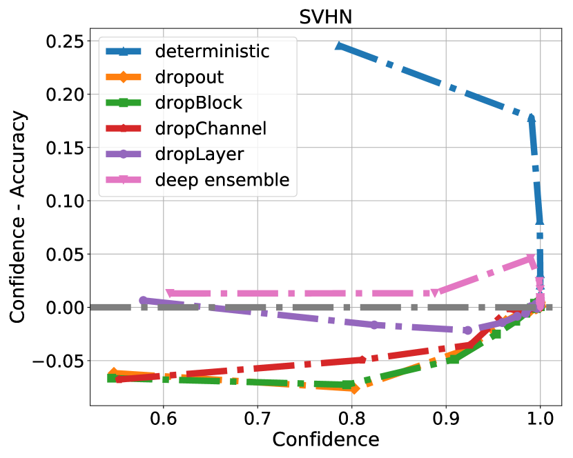
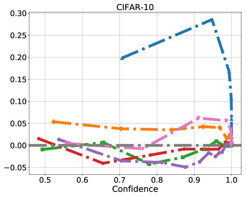
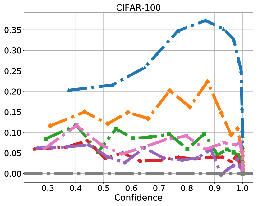
Figure 1: Reliability diagrams of predictions produced by difference models. Models with structured dropout produce better calibrated predictions, as evidenced by curves that are closer to the x-axis.

As seen from Table 1 and Figure 1, MC dropLayer and MC dropChannel offer the best confidence calibration, together with good accuracy. Remarkably, both of these methods achieve even lower ECE than that of deep ensemble, which requires $5$ times more computational resource. We also find that MC dropLayer tends to be less sensitive to the choice of dropout rate (see Appendix A). While MC dropout is able to achieve comparable performance to the proposed methods on the SVHN dataset, the confidence values produced are much worse in terms of every evaluation metric for both of the CIFAR datasets. Furthermore, comparatively, the performance of MC dropout becomes worse as the dataset used becomes more difficult, from SVHN to CIFAR-100. Lastly, as evident from moderately increased classification accuracy over deterministic models, all types of dropout methods can be incorporated into architectures for uncertainty estimates with no accuracy penalty.

Discussion  We believe the relatively good performance of MC dropout on SVHN compared to the CIFAR datasets is because the former task is relatively easier and thus the model can still predict accurately at an aggressive dropout rate of $0.35$ at which even regular dropout can produce acceptably diverse sampled models. In contrast, as observed during our experiments, while using larger dropout rates for the more difficult CIFAR datasets can lead to more calibrated predictions, classification accuracy and NLL suffer significantly (see Appendix A). Hence, naively increasing the dropout rate does not always lead to better performance. Furthermore, we believe the results for MC dropBlock can be improved by optimizing the choice of block size. A pre-fixed block size of $3\times 3$ can be too small for the upstream convolutional layers where the size of feature maps are much larger than the block size, and too large for the last few downstream layers where the feature maps are comparable to the block size. Indeed, we observe in our experiments that when larger dropout rates are used for MC dropBlock, classification accuracy drops drastically, indicating the possibility that too much information is discarded to make a good prediction (see Appendix A).

4.2 Ensemble Diversity

In order to gain more insight about the improvement obtained with structured dropout, we investigate the diversity of the models sampled from dropout at all scales. We illustrate using models trained on CIFAR-10. For a fair comparison, we fix the dropout rate for all models to $0.1$, so that all the models trained with different types of dropout have the same complexity in terms of total effective number of parameters. We note however since deep ensemble does not use dropout, it effectively has a larger capacity than all the dropout-trained models for this analysis.

As seen from Figure 2 (Left), the gain in accuracy by having a larger number of test-time MC samples is much smaller for regular dropout compared to that of structured dropout techniques. This plot also provides some insights about the average ambiguity (or model diversity) because, according to Equation 2, average ambiguity is the difference between the average MSE of an individual model (which corresponds to the average accuracy of the “one model ensemble”, the left-most points on the curves of Figure 2 (Left)) and the MSE of the ensemble of models. Recall that MSE is highly correlated with classification accuracy. Thus the amount of increase in the curves of Figure 2 (Left) are reflective of the amount of model diversity, suggesting structured dropout techniques promote more diversity than dropout. We also see the improvement in accuracy obtained through deep ensemble, which again is a computationally expensive strategy that relies on multiple models trained with different random initializations and SGD intantiations. Surprisingly, the net gain in accuracy for models obtained through structured dropout is greater than the gain offered by deep ensembling. In terms of ECE, from Figure 2 (Right), when the number of models in the ensemble is one, all approaches are very poorly calibrated. However, ECE decreases sharply as the number of models in the ensemble increases. The improvement is much less significant for MC dropout, likely due to limited diversity. Again, the relative improvements for models sampled with structured dropout exceeds that of the deep ensemble. In fact, with five models in the ensemble, MC dropBlock achieves a calibration error lower than deep ensemble.

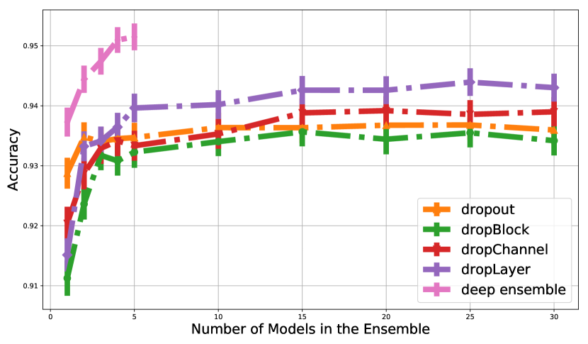
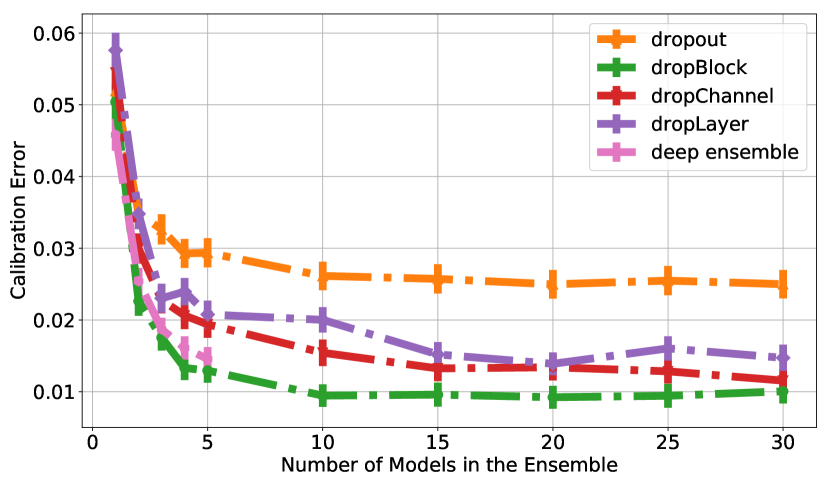
Figure 2: Test accuracy (left) and ECE (right) against number of models for ensemble prediction at test time on CIFAR-10. For varioius versions of dropout, this corresponds to the number of different MC dropout instantiations at test time of the same model. For deep ensemble, the x-axis is the number of models trained with random initializations and SGD. The error bars are bootstrap estimated standard deviation on the testset. Models trained with structured dropout methods benefit much more from ensemble averaging.

Table 2: Interrater Agreement (IA) of models with diffrent types of dropout with $0.1$ dropout rate. The lower the IA, the more diverse the predictions of the models. Dropout produces models with larger IA, hence less model diversity, than structured dropout techniques.

Dataset Dropout DropBlock DropChannel DropLayer Deep Ensemble SVHN $0.723\pm 0.004$ $\boldsymbol{0.582\pm 0.004}$ $0.670\pm 0.005$ $0.746\pm 0.008$ $\boldsymbol{0.632}$ CIFAR-10 $0.696\pm 0.003$ $0.568\pm 0.005$ $0.615\pm 0.006$ $\boldsymbol{0.512\pm 0.013}$ $\boldsymbol{0.586}$ CIFAR-100 $0.790\pm 0.002$ $0.708\pm 0.003$ $\boldsymbol{0.690\pm 0.003}$ $0.720\pm 0.006$ $\boldsymbol{0.660}$

In addition to ambiguity, there have been numerous performance measures proposed in the ensemble learning community zhou2012ensemble to explicitly quantify the diversity of model ensembles. In this paper, we use the Interrater Agreement (IA) as the performance measure kuncheva2003measures . It is defined as:

$$\kappa=1-\frac{\frac{1}{T}\sum^{n}_{k=1}\rho(x_{k})(T-\rho(x_{k}))}{n(T-1)\bar{p}(1-\bar{p})},$$ (6)

where $T$ corresponds to the number of models (individual classifiers), $n$ corresponds to the total number of samples in the test set, $\rho(x_{k})$ is the number of classifiers that classifies the $k$-th sample correctly, and $\bar{p}$ is the average classification accuracy of the individual classifiers. As a measure of agreement across individual classifiers, $\kappa=1$ if the classifiers perfectly agree on the test set. The smaller the $\kappa$, the less the individual classifiers agree, and the more the model diversity. Table 2 summarizes IR for sampled models trained on different datasets through dropout at different scales. We also compare the results with deep ensemble. The number of models in the ensemble is fixed to be 5 for all approaches. The standard deviation estimates for the dropout methods were obtained through empirically sampling 5 model ensembles. The IA for MC dropout is much higher than that of the different structured dropout techniques. Similar to our observations above, compared to deep ensemble, structured dropout can yield ensembles that are as diverse as the computationally expensive method of deep ensemble. In fact, the IA of MC DropLayer with CIFAR-10 is smaller than that of deep ensemble. However, for diversity achieved by structured dropout, there is no technique that is overall superior. For example, MC DropLayer achieves high IA scores on the SVHN dataset, whereas yields better diversity on CIFAR-100. We suspect this pattern is influenced by the choice of the neural network architecture and dataset. For example, for the SVHN dataset, we use a relatively shallow, 18-layer, neural network, which might constrain the achievable diversity using a specific dropout strategy.

4.3 Bayesian Active Learning

To further demonstrate the merit of the proposed use of structured dropout for confidence calibration, we consider the downstream task of Bayesian active learning on the CIFAR-10 dataset. In general, active learning involves first training on a small amount of labeled data. Then, an acquisition function based on the outputs of models is used to select a small subset of unlabeled data so that an oracle can provide labels for these queried data. Samples that a model is the least confident about are usually selected for labeling, in order to maximize the information gain. The model is then retrained with the additional labeled data that is provided. The above process can be repeated until a desired accuracy is achieved or the labeling resources are exhausted.

In our experiment, we train models with structured dropout at different scales using the identical setup as described in the beginning of this section, except that only $2000$ training samples are used initially. To match up model capacity, the dropout rate is set to $0.1$ for all methods. After the first iteration, we acquire $1000$ samples from a pool of "unlabeled" data, and combine the acquired samples with the original set of labeled images to retrain the models. Following Gal et al. gal2017deep , we consider three acquision functions: Max Entropy, $\mathbb{H}[y|\boldsymbol{x},\mathcal{D}_{train}]=-\sum_{c}p(y=c|\boldsymbol{x},\mathcal{D}_{train})\log p(y=c|\boldsymbol{x},\mathcal{D}_{train})$, the BALD metric (Bayesian Active Learning by Disagreement), $\mathbb{I}[y,\boldsymbol{w}|\boldsymbol{x},\mathcal{D}_{train}]=\mathbb{H}[y|\boldsymbol{x},\mathcal{D}_{train}]-\mathbb{E}_{p(\boldsymbol{w}|\mathcal{D}_{train})[\mathbb{H}[y|\boldsymbol{x},\boldsymbol{w}]]}$, and the Variation Ratios metric, $\text{variation-ratio}[\boldsymbol{x}]=1-\max_{y}p(y,\boldsymbol{x},\mathcal{D}_{train})$. We repeat the acquisition process 9 times so that in the last iteration, the training set contains $10000$ images. Test accuracies are calculated before each acquisition phase. To mimic a real world scenario in which number of labeled samples is small, we do not use a validation set, and the accuracies reported for this experiment correspond to the last-epoch accuracies. Due to the small training set and hence larger variance in results, we repeat the experiment 5 times and compute the mean accuracies.

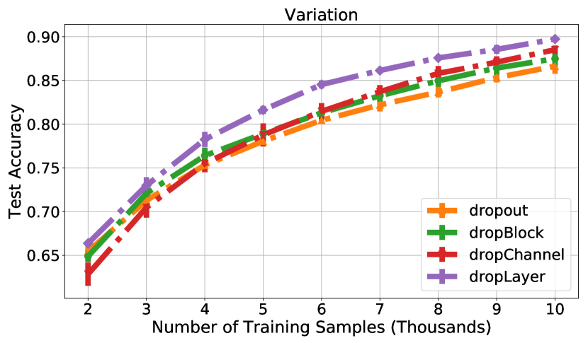
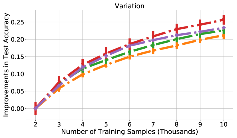
Figure 3: Left: Test accuracy against number of training samples for models with different methods of dropout and Variation Ratios as the acquisition function on CIFAR-10. Right: Relative improvements in test accuracy over that of the first iteration with different methods of dropout. MC dropout yields the least improvements of all the methods.

Figure 3 shows the test accuracy against number of training samples for different models, with Variation Ratios used as the acquisition function. It can be seen that, after the first iteration when all $2000$ training images are randomly selected, the test accuracy using MC dropout is on par with that of other methods. However, as more labeled data are added, the relative increase in accuracy is more significant for models using structured dropout compared to that of using regular dropout. For instance, the ulitmate increase in accuracy with MC dropout is $21.1\pm 1.1\%$ compared to that of $25.7\pm 1.4\%$ when using MC dropChannel. This suggests that the uncertainty estimates obtained with structured dropout are more useful for assessing "what the model doesn’t know", thereby allowing for the selection of samples to be labeled in a way that better helps improve performance. Similar trends are observed for the other acquisition functions (see Appendix B). Of the three acquisition functions, Max Entropy and Variation Ratios seem to be more effective in our experiment.

5 Conclusion and Future Work

We reinterpret MC dropout as ensemble averaging strategy, and attribute the calibration error in confidence estimates to a lack of diversity of sampled models. As we demonstrate in our experiments, structured dropout, which is simple-to-implement and computationally efficient, can promote model diversity and improve calibration. The gain in performance, however, depends on the architecture, the task, the dropout rate and the structured dropout strategy.

We are interested in further exploring several directions. Firstly, there are many other architectures for implementing MC dropLayer larsson2016fractalnet ; xie2017aggregated , and we have only considered ResNet. Moreover, we used a constant dropout rate in our experiments, even though one can vary dropout rates across NNs huang2016deep or incorporate dropout rate scheduling ghiasi2018dropblock . How this impacts calibration is an open question. Lastly, we have only considered structured dropout in the context of CNNs, with application to computer vision tasks. We believe this idea can be extended beyond CNNs.

Appendix A: Performance of Uncertainty Estimates Against Dropout Rate

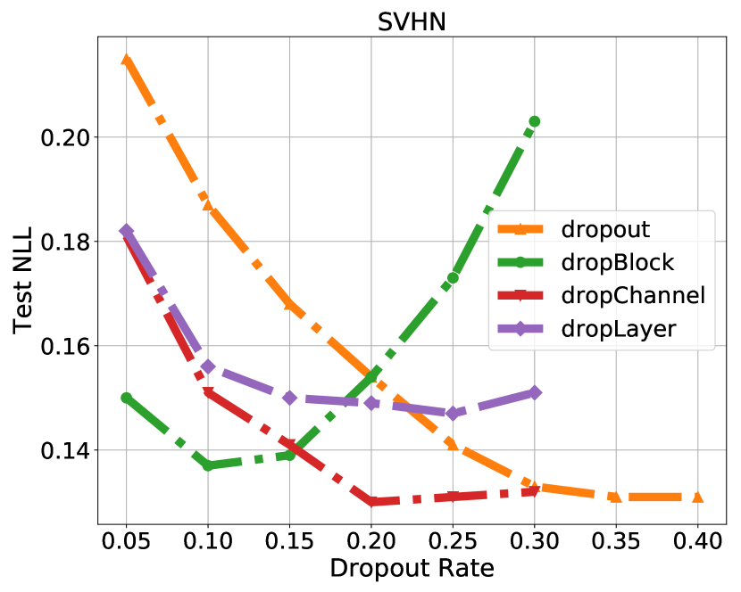
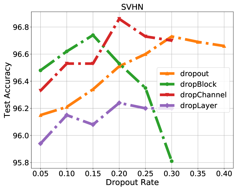
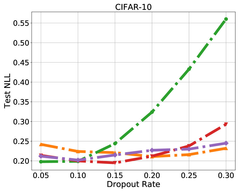
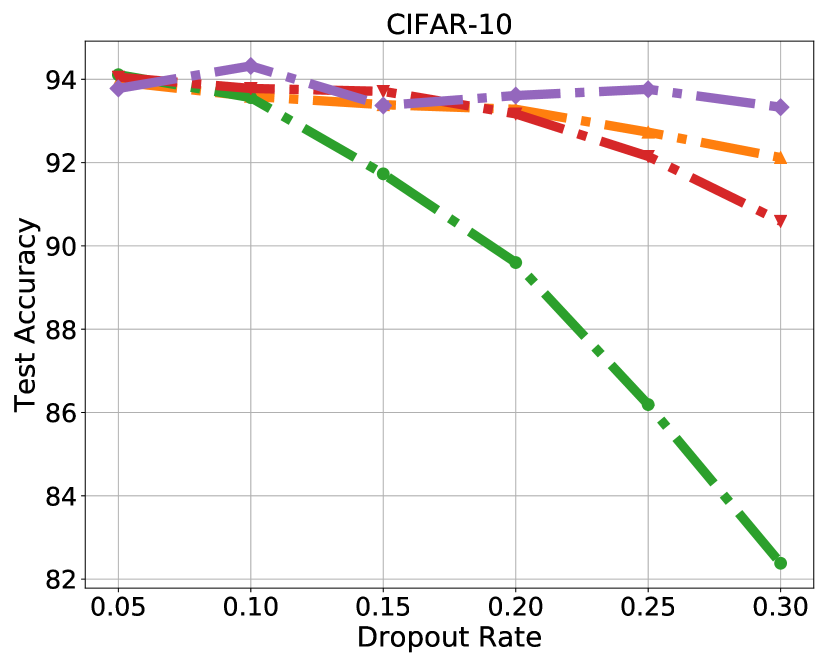
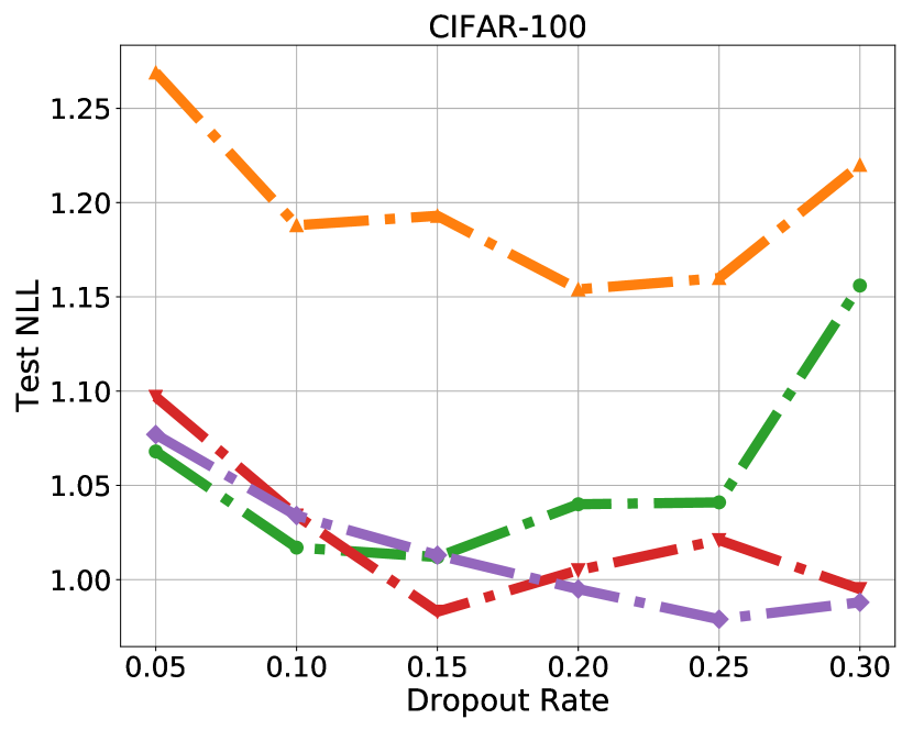
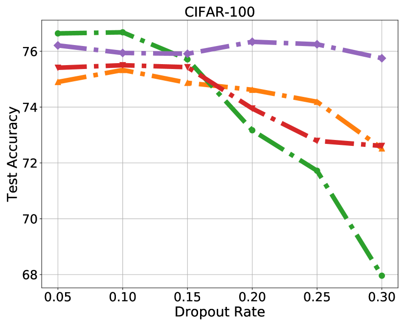
Figure 4: Plots of test time NLL (Left) and accuracy (Right) against dropout rate for models trained with different types of dropout on the SVHN, CIFAR-10 and CIFAR-100 datasets. Models trained with structured dropout can achieve better NLL performance, particularly for moderate values of the dropout rate. DropLayer is the least sensitive to the choice of dropout rate with respect to NLL. Interestingly, the NLL drastically increases after minima on all three datasets for dropBlock, suggesting the possibility that the block size for dropBlock may be too large towards later convolutional layers when the size of feature maps are comparable to that of block size.

Appendix B: Additional Results with Active Learning

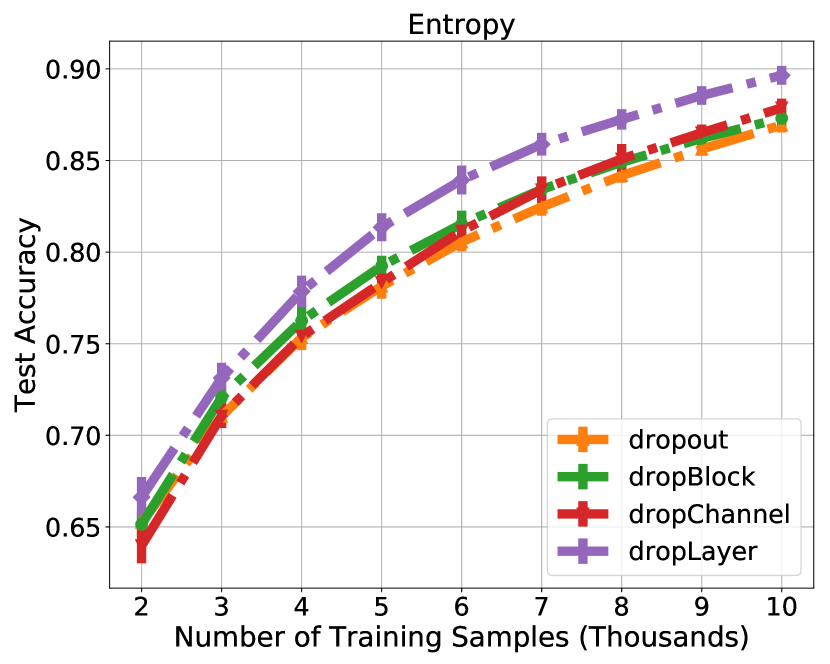
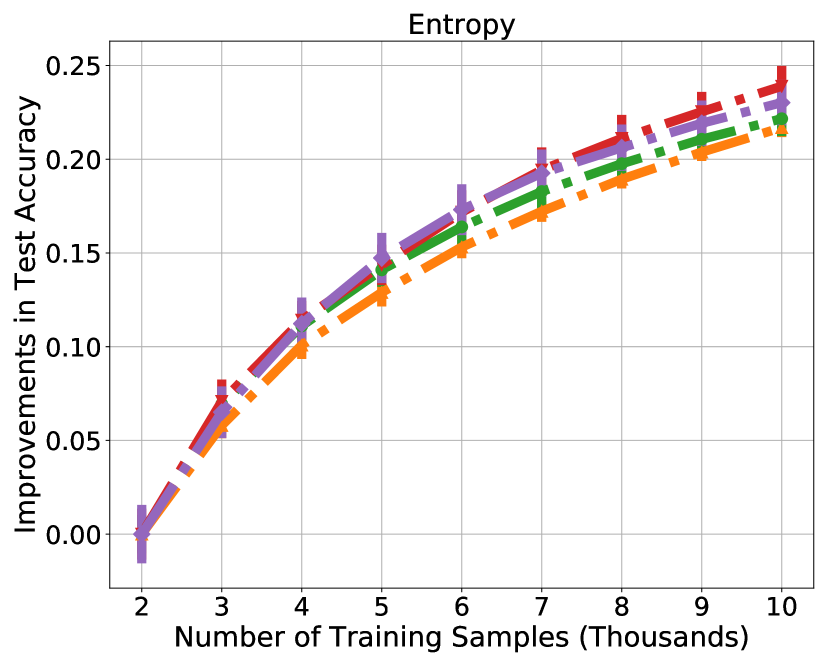
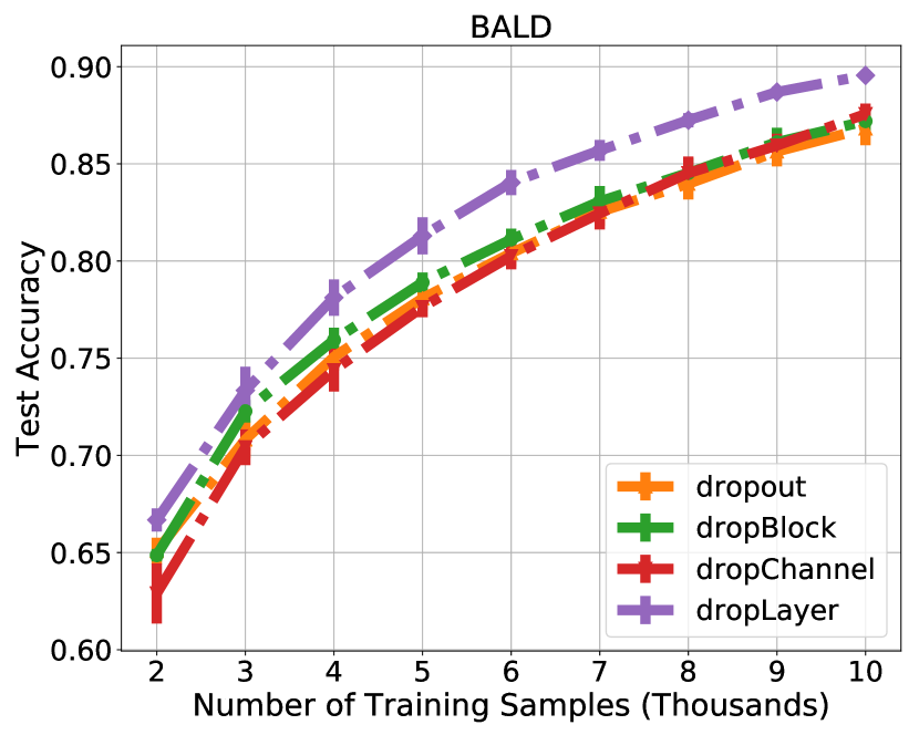
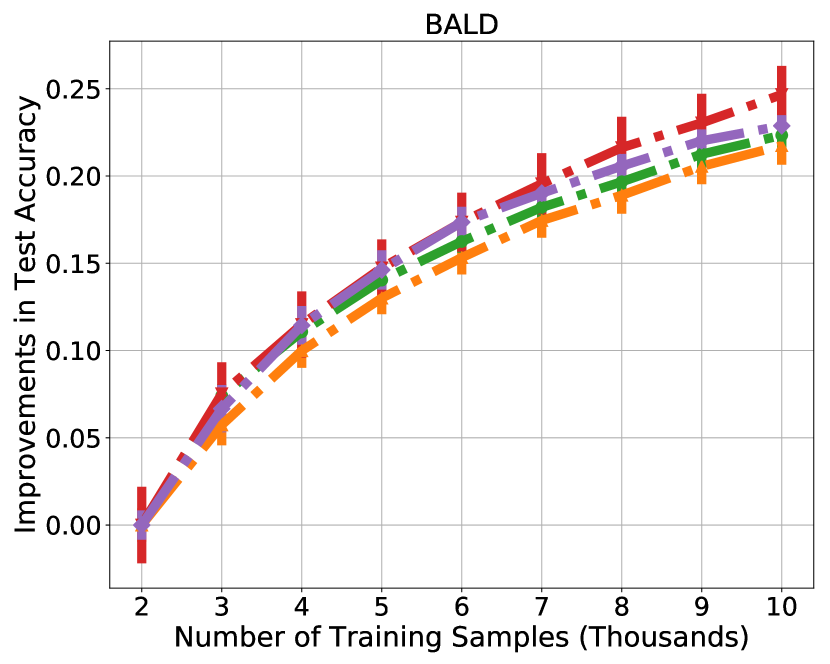
Figure 5: Left: Test accuracy against number of training samples for models with different methods of dropout and Max Entropy (Above) / BALD (Below) as the acquisition function on CIFAR-10. Right: Relative improvements in test accuracy over that of the first iteration with different methods of dropout. Similar to results obtained with Variation Ratios, MC dropout yields the least improvements of all the methods.

References

- (1) Léonard Blier and Yann Ollivier. The description length of deep learning models. In Advances in Neural Information Processing Systems, pages 2216–2226, 2018.
- (2) Charles Blundell, Julien Cornebise, Koray Kavukcuoglu, and Daan Wierstra. Weight uncertainty in neural network. In International Conference on Machine Learning, pages 1613–1622, 2015.
- (3) Tianqi Chen, Emily Fox, and Carlos Guestrin. Stochastic gradient hamiltonian monte carlo. In International conference on machine learning, pages 1683–1691, 2014.
- (4) Yarin Gal and Zoubin Ghahramani. Dropout as a bayesian approximation: Representing model uncertainty in deep learning. In international conference on machine learning, pages 1050–1059, 2016.
- (5) Yarin Gal and Zoubin Ghahramani. A theoretically grounded application of dropout in recurrent neural networks. In Advances in neural information processing systems, pages 1019–1027, 2016.
- (6) Yarin Gal, Jiri Hron, and Alex Kendall. Concrete dropout. In Advances in Neural Information Processing Systems, pages 3581–3590, 2017.
- (7) Yarin Gal, Riashat Islam, and Zoubin Ghahramani. Deep bayesian active learning with image data. In Proceedings of the 34th International Conference on Machine Learning-Volume 70, pages 1183–1192. JMLR. org, 2017.
- (8) Xavier Gastaldi. Shake-shake regularization. arXiv preprint arXiv:1705.07485, 2017.
- (9) Yonatan Geifman, Guy Uziel, and Ran El-Yaniv. Bias-reduced uncertainty estimation for deep neural classifiers. International Conference on Learning Representations, 2019.
- (10) Golnaz Ghiasi, Tsung-Yi Lin, and Quoc V Le. Dropblock: A regularization method for convolutional networks. In Advances in Neural Information Processing Systems, pages 10727–10737, 2018.
- (11) Wenbo Gong, Yingzhen Li, and José Miguel Hernández-Lobato. Meta-learning for stochastic gradient mcmc. International Conference on Learning Representations, 2019.
- (12) Ian J Goodfellow, David Warde-Farley, Mehdi Mirza, Aaron Courville, and Yoshua Bengio. Maxout networks. International Conference on Machine Learning, 2013.
- (13) Alex Graves. Practical variational inference for neural networks. In Advances in neural information processing systems, pages 2348–2356, 2011.
- (14) Chuan Guo, Geoff Pleiss, Yu Sun, and Kilian Q Weinberger. On calibration of modern neural networks. In Proceedings of the 34th International Conference on Machine Learning-Volume 70, pages 1321–1330. JMLR. org, 2017.
- (15) Kaiming He, Xiangyu Zhang, Shaoqing Ren, and Jian Sun. Deep residual learning for image recognition. In Proceedings of the IEEE conference on computer vision and pattern recognition, pages 770–778, 2016.
- (16) Kaiming He, Xiangyu Zhang, Shaoqing Ren, and Jian Sun. Identity mappings in deep residual networks. In European conference on computer vision, pages 630–645. Springer, 2016.
- (17) Gao Huang, Yu Sun, Zhuang Liu, Daniel Sedra, and Kilian Q Weinberger. Deep networks with stochastic depth. In European conference on computer vision, pages 646–661. Springer, 2016.
- (18) Pavel Izmailov, Dmitrii Podoprikhin, Timur Garipov, Dmitry Vetrov, and Andrew Gordon Wilson. Averaging weights leads to wider optima and better generalization. Conference on Uncertainty in Artificial Intelligence, 2018.
- (19) Alex Kendall and Yarin Gal. What uncertainties do we need in bayesian deep learning for computer vision? In Advances in neural information processing systems, pages 5574–5584, 2017.
- (20) Durk P Kingma, Tim Salimans, and Max Welling. Variational dropout and the local reparameterization trick. In Advances in Neural Information Processing Systems, pages 2575–2583, 2015.
- (21) Alex Krizhevsky. Learning multiple layers of features from tiny images. Technical report, Citeseer, 2009.
- (22) Anders Krogh and Jesper Vedelsby. Neural network ensembles, cross validation, and active learning. In Advances in neural information processing systems, pages 231–238, 1995.
- (23) Volodymyr Kuleshov and Percy S Liang. Calibrated structured prediction. In Advances in Neural Information Processing Systems, pages 3474–3482, 2015.
- (24) Ludmila I Kuncheva and Christopher J Whitaker. Measures of diversity in classifier ensembles and their relationship with the ensemble accuracy. Machine learning, 51(2):181–207, 2003.
- (25) Balaji Lakshminarayanan, Alexander Pritzel, and Charles Blundell. Simple and scalable predictive uncertainty estimation using deep ensembles. In Advances in Neural Information Processing Systems, pages 6402–6413, 2017.
- (26) Gustav Larsson, Michael Maire, and Gregory Shakhnarovich. Fractalnet: Ultra-deep neural networks without residuals. International Conference on Learning Representations, 2017.
- (27) Yixuan Li, Jason Yosinski, Jeff Clune, Hod Lipson, and John E Hopcroft. Convergent learning: Do different neural networks learn the same representations?
- (28) Christos Louizos and Max Welling. Multiplicative normalizing flows for variational bayesian neural networks. In Proceedings of the 34th International Conference on Machine Learning-Volume 70, pages 2218–2227. JMLR. org, 2017.
- (29) Yi-An Ma, Tianqi Chen, and Emily Fox. A complete recipe for stochastic gradient mcmc. In Advances in Neural Information Processing Systems, pages 2917–2925, 2015.
- (30) David JC MacKay. A practical bayesian framework for backpropagation networks. Neural computation, 4(3):448–472, 1992.
- (31) Wesley Maddox, Timur Garipov, Pavel Izmailov, Dmitry Vetrov, and Andrew Gordon Wilson. A simple baseline for bayesian uncertainty in deep learning. arXiv preprint arXiv:1902.02476, 2019.
- (32) Mahdi Pakdaman Naeini, Gregory Cooper, and Milos Hauskrecht. Obtaining well calibrated probabilities using bayesian binning. In Twenty-Ninth AAAI Conference on Artificial Intelligence, 2015.
- (33) Radford M Neal. Bayesian learning for neural networks, volume 118. Springer Science & Business Media, 2012.
- (34) Yuval Netzer, Tao Wang, Adam Coates, Alessandro Bissacco, Bo Wu, and Andrew Y Ng. Reading digits in natural images with unsupervised feature learning. 2011.
- (35) Hippolyt Ritter, Aleksandar Botev, and David Barber. A scalable laplace approximation for neural networks. International Conference on Learning Representations, 2018.
- (36) Nitish Srivastava, Geoffrey Hinton, Alex Krizhevsky, Ilya Sutskever, and Ruslan Salakhutdinov. Dropout: a simple way to prevent neural networks from overfitting. The Journal of Machine Learning Research, 15(1):1929–1958, 2014.
- (37) Jonathan Tompson, Ross Goroshin, Arjun Jain, Yann LeCun, and Christoph Bregler. Efficient object localization using convolutional networks. In Proceedings of the IEEE Conference on Computer Vision and Pattern Recognition, pages 648–656, 2015.
- (38) Dimitris Tsipras, Shibani Santurkar, Logan Engstrom, Alexander Turner, and Aleksander Madry. Robustness may be at odds with accuracy. International Conference on Learning Representations, 2019.
- (39) Andreas Veit, Michael J Wilber, and Serge Belongie. Residual networks behave like ensembles of relatively shallow networks. In Advances in neural information processing systems, pages 550–558, 2016.
- (40) Li Wan, Matthew Zeiler, Sixin Zhang, Yann Le Cun, and Rob Fergus. Regularization of neural networks using dropconnect. In International conference on machine learning, pages 1058–1066, 2013.
- (41) Liwei Wang, Lunjia Hu, Jiayuan Gu, Zhiqiang Hu, Yue Wu, Kun He, and John Hopcroft. Towards understanding learning representations: To what extent do different neural networks learn the same representation. In Advances in Neural Information Processing Systems, pages 9584–9593, 2018.
- (42) Max Welling and Yee W Teh. Bayesian learning via stochastic gradient langevin dynamics. In Proceedings of the 28th international conference on machine learning (ICML-11), pages 681–688, 2011.
- (43) Anqi Wu, Sebastian Nowozin, Edward Meeds, Richard E Turner, José Miguel Hernández-Lobato, and Alexander L Gaunt. Deterministic variational inference for robust bayesian neural networks. International Conference on Learning Representations, 2018.
- (44) Saining Xie, Ross Girshick, Piotr Dollár, Zhuowen Tu, and Kaiming He. Aggregated residual transformations for deep neural networks. In Proceedings of the IEEE conference on computer vision and pattern recognition, pages 1492–1500, 2017.
- (45) Zhi-Hua Zhou. Ensemble methods: foundations and algorithms. Chapman and Hall/CRC, 2012.