Building a Benchmark Dataset and Classifiers for Sentence-Level Findings in AP Chest X-rays

Abstract

Chest X-rays are the most common diagnostic exams in emergency rooms and hospitals. There has been a surge of work on automatic interpretation of chest X-rays using deep learning approaches after the availability of large open source chest X-ray dataset from NIH. However, the labels are not sufficiently rich and descriptive for training classification tools. Further, it does not adequately address the findings seen in Chest X-rays taken in anterior-posterior (AP) view which also depict the placement of devices such as central vascular lines and tubes. In this paper, we present a new chest X-ray benchmark database of 73 rich sentence-level descriptors of findings seen in AP chest X-rays. We describe our method of obtaining these findings through a semi-automated ground truth generation process from crowdsourcing of clinician annotations. We also present results of building classifiers for these findings that show that such higher granularity labels can also be learned through the framework of deep learning classifiers.

Index Terms—  chest X-rays, AP view, datasets, deep learning networks, ensemble networks

1 Introduction

Chest X-rays are the most common imaging exams being conducted in emergency rooms. Recently, a number of researchers have begun automated interpretation of chest X-rays, focusing on posterior-anterior (PA) views and limited number of labels of high granularity such as opacity or consolidation.[1, 2, 3]. If machines are to assist radiologists through automated interpretation, it is important to expand the number of findings as well as refine them to incorporate location, laterality, character and other information so that automated report generation may one day become possible. Further, the viewpoints should be expanded to cover anterior-posterior (AP) views as well which are generally taken to aid in the diagnosis of acute and chronic conditions in intensive care units in hospitals. Although the AP view is lower in quality to PA view, this is often the only mode in which sick patients can be imaged for problems in lungs, bony thoracic cavity, mediastinum, and great vessels. The resulting images often depict multiple types of findings such as anatomical findings, technical assessment problems, and tubes/lines placement issues as shown in Figure 1.

Currently no labeled datasets that cover the list of possible findings seen in AP chest X-rays. The large open source chest X-ray dataset provided from NIH[2] covers only discrete anatomical findings. Hence existing approaches have either ignored the viewpoint during training [1, 2] or focused on PA views only[3].

Fig. 1: Illustration of spatial overlap between labels relating to lines and tubes and anatomical findings.

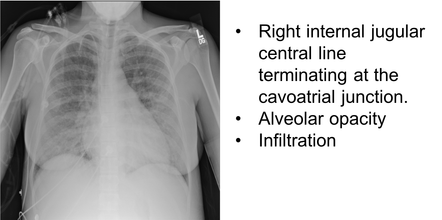
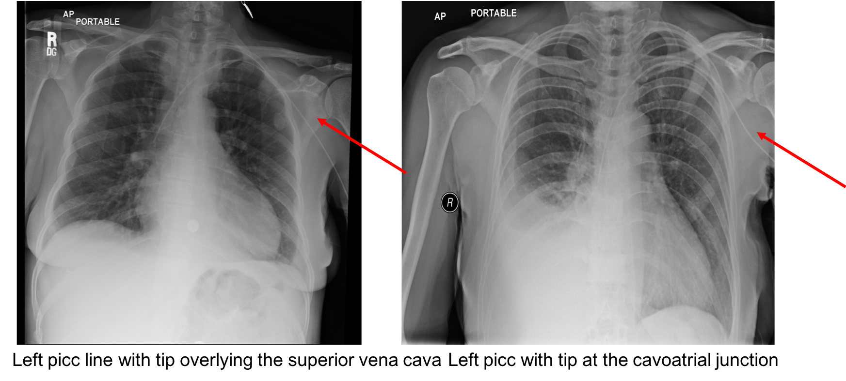
Chest X-rays also depict spatially and semantically overlapping findings for which simple labels describing only the core finding are not sufficient to build robust classifiers. Figure 1 illustrates the difficulty of detecting spatially overlapping findings in AP chest X-rays. Here, the findings of ”infiltration”, ”alveolar opacity”, and positioning of ”right internal jugular line at the cavoatrial junction” are all within the same spatial vicinity. When feature regions of two different class labels spatially overlap, the classifiers often select weights that bias towards the label with larger training data. Figure 2 shows the specificity of labels problem with AP chest X-rays where semantic overlap between findings need to be carefully distinguished by describing not only the core findings but also the placement. Here the classification method needs to be fine grained to recognize the difference in the similarity of the labels referring to the same device but placed at different locations in the body. This requires higher precision in deriving the labels themselves.

In the work on chest X-rays so far, not enough attention has been paid to the choice of labels for the classifiers. Although about half of the NIH dataset consists of AP chest X-rays (44,812 images), the labels currently provided only cover anatomical findings without elaborating on modifiers such as laterality, location or severity which affect visual appearance and hence the classification accuracies. Fresh annotation efforts have also begun but focused on a single finding such as the pneumonia dataset recently provided by RSNA-Kaggle challenge[4]. Since all AP chest X-ray findings are also documented in radiology reports, automatic interpretation algorithm must support AP chest X-ray imaging. Hence there is a need to derive higher granularity labels for AP Chest X-ray imaging.

Fig. 2: Illustration of semantic overlap in labels both referring to different positioning of left picc lines.

Fig. 3: Illustration of structured template used to collect radiology report to derive the labels.

In this paper we present a benchmark dataset of AP chest X-rays originally derived from NIH dataset but relabeled for higher granularity findings in AP chest X-rays. The labels are derived from a semi-automatic curation process that involves crowd-sourcing of clinician read reports through ease-of-use user interfaces followed by automated text clustering and semantic grouping, and final clinician verification. To obtain sufficient granularity of description, sentence level labels are retained. Such labels also facilitate the production of automated reports as they can be directly used to form the report. We also address the problem of building classifiers for such higher granularity findings by exploring two architectures, one based on conventional deep learning and another hybrid deep learning formulation to exploit the greater feature selection and explain capability of ensemble classifiers. These results show that such higher granularity findings in AP chest X-rays can also be learned by the state-of-the-art classifiers.

Fig. 4: Illustration of results of semantic clustering of report sentences.

Fig. 5: Illustration of label data reduction through successive processing.

2 Label generation for AP Chest X-rays

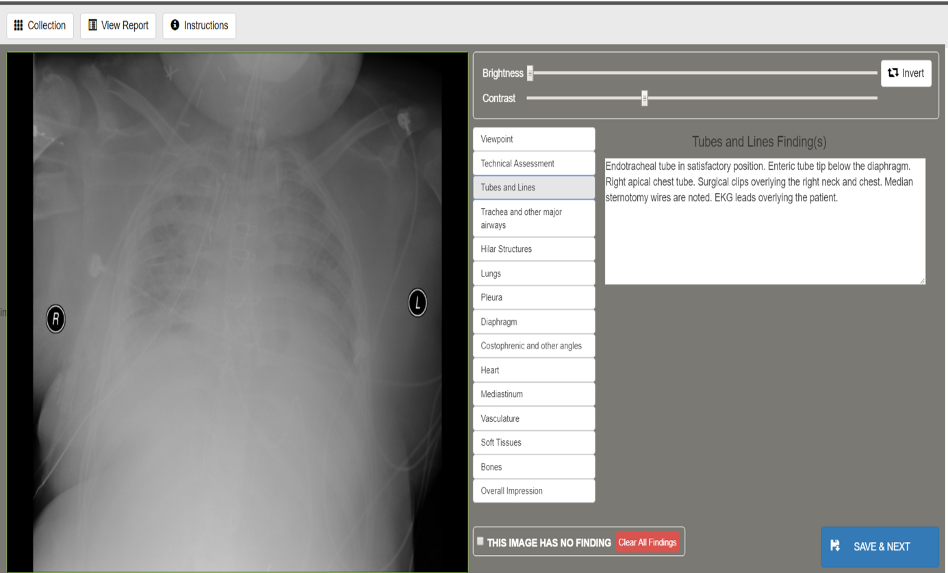
The NIH dataset consists of 112,121, images with 44,812 images in AP view from 9061 patients. To generate the labeled dataset for AP chest X-rays, we sampled the dataset so that at least one AP chest X-ray image was selected from all patients to obtain a total of 16910 unique images for re-annotation. To rapidly annotate the large dataset and list of possible findings in AP chest X-rays, we developed a web-based crowd-sourcing annotation system and recruited over 42 radiologists around the country to perform the annotation. In collecting the annotation, we simulated a radiology read setup in a hospital by providing a templated report form to the radiologists shown in Figure 3. As can be seen by the template, it allows radiologists to describe all major structures seen in chest X-rays as well as any device artifacts including lines and tubes. Further, technical assessment was also captured in addition to structured labeling of viewpoints. The free text form within these templated sections allowed radiologists freedom to describe or dictate the findings relatively freely to rapidly complete a report (20 images/per hour was the observed speed) without requiring the selection of discrete labels.

2.1 Sentence clustering for label generation

The resulting reports generated nearly 45000 sentences of which 17000 unique sentences were discovered after normalization by removing the stop words, small typos, case differences, etc. while still maintaining the order of the words. Clustering was then attempted within sentences coming from the same report template section. The distance metric chosen for clustering measured the extent of overlap of words between two sentences with and without keeping the order of the words. The pairwise similarity between two sentences $S=<s_{1}s_{2}...s_{K}>$ of K words, and $T=<t_{1}t_{2}...t_{N}>$ of N words was defined as:

$$d(S,T)=max\{d_{unordered}(S,T),d_{ordered}(S,T)\}$$ (1)

where $d_{unordered}(S,T)$ is given by

$$d_{unordered}(S,T)=\frac{2*|S\cap T|}{|S\cup T|}$$ (2)

where $|S\cap T|$ is the number of words common between $S$ and $T$ and $|S\cup T|$ is the total length of the two strings in words.

The ordered score $d_{ordered}(S,T)$ is the ordered similarity computed by a string matching algorithm called the longest common subfix (LCF) algorithm [5] given by $d_{ordered}(S,T)=<p_{1}p_{2}...p_{L}>$ , where L is the largest subset of words from S that found a partial match in T and $p_{i}$ is a partial match of a word $s_{i}\in S$ to a word in T. A word $s_{i}$ in S is said to partially match a word $t_{j}$ in T if it shares a maximum length common prefix $p_{i}$ such that $\frac{|p_{i}|}{\mbox{max}\{|s_{i}|,|t_{j}|\}}>\tau$. If we make the threshold $\tau=1.0$ , this reduces to the case of finding exact matches to words of S. Note that this formulation is different from the conventional longest common subsequence (LCS) string matching as there is an emphasis on character grouping into words and the use of word prefixes to relate words in the English language. This algorithm uses dynamic programming alignment at the words level using word prefixes and allows for gaps and insertions while preserving the word order. The algorithm also uses other enhancements for negation pattern finding, and abbreviation expansions as described in [5].

The ordered score $d_{ordered}$ can be computed using dynamic programming alignment algorithm by keeping an array $C[i,j]$ to calculate the score of matching a fragment of $S$ up to the ith word and fragment of $T$ up to the jth word. We then update the dynamic programming matrix according to the algorithm shown in Algorithm $1$. Here $p_{max}(i,j)$ is the longest prefix of the strings $(s_{i},t_{j})$ and $\delta$ is a mismatch penalty, which controls the separation between matched words and prevents words that are too far apart in a sentence from being associated with the target sentence. Using this algorithm, $S$ is said to match sentence $T$ if $\frac{|LCF(S,T)|}{|S|}\geq\Gamma$ for some threshold $\Gamma$. The choice of $\delta$ and $\Gamma$ affect the closeness of the match and were chosen to meet specified criteria for precision and recall based on an ROC curve analysis on labeled collection.

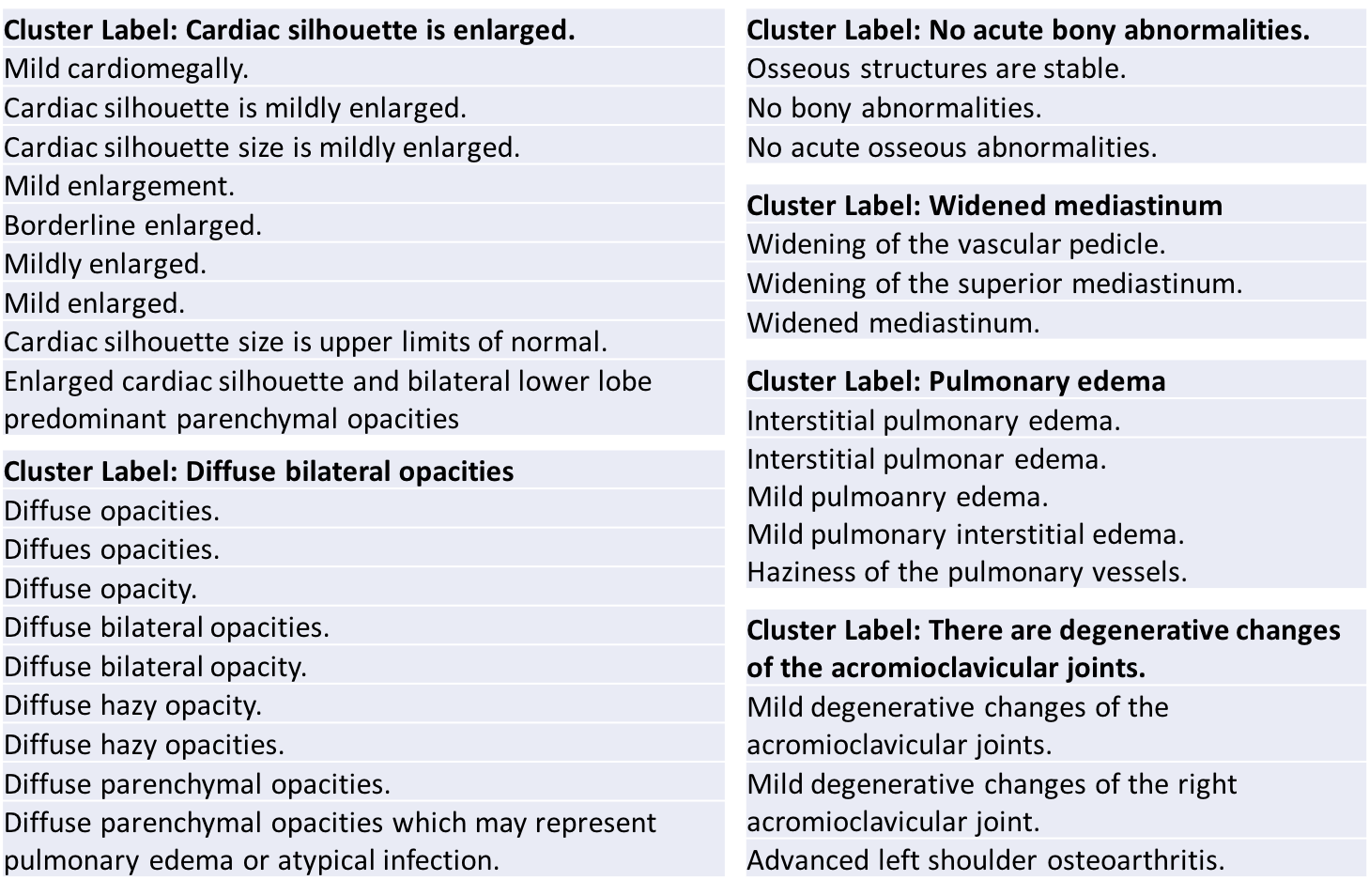
Figure 4 shows the results of applying the similarity score $d(S,T)$ on a variety of sentences found in the generated reports. It can be seen that the algorithm spots sentences with similar meanings without a deep understanding of their linguistic origins. The algorithm uses other enhancements for handling negations and abbreviation expansions which are skipped here for brevity.

Algorithm 1 Longest Common Subfix Algorithm

LCF(S,T):

1:  Input/Output Input: two strings (S,T). Output: an alignment score.

2:  Initialize $c[i,0]=0,c[0,j]=0,0\leq i\leq K,0\leq j\leq N$.

3:  Iterate for $(1\leq i\leq K)$           for $(1\leq j\leq N)$               $\rho_{ij}=\frac{|p_{max}(i,j)|}{\mbox{max}\{|s_{i}|,|t_{j}|\}}$                If $C[i-1,j-1]+\rho_{ij}>C[i-1,j]$ and                      $C[i-1,j-1]+\rho_{ij}>C[i,j-1]$                          $C[i,j]=C[i-1,j-1]+\rho_{ij}$                else                     if $(C[i-1,j]+\rho_{ij}>C[i,j-1]$                          $C[i,j]=C[i-1,j]-\delta$                     else                          $C[i,j]=C[i,j-1]-\delta$

To perform clustering, all unique sentences belonging to a section heading across reports are collected and lexicographically ordered. Starting from the first sentence, each successive sentence is added to the cluster if its LCF distance is within a threshold with respect to all previous members. The first sentence that violates this constraint becomes the start of a new cluster. This method of grouping brings out the lexical similarity in the sentences as shown in Figure 4. Here a representative sentence from that group is used to denote the cluster. Using this process, the total sentences to examine reduced from 40,000 to about 458 cluster representatives as shown in Figure 5 based on the number of clusters produced (also 458). The semantic merging of these labels is then done manually by radiologists on this reduced dataset to further group the labels into 113 semantic groups. In doing the grouping, the radiologists kept the distinction of location, laterality and severity as those cause changes in visual appearance. By retaining all those clusters with more than 50 images per cluster, we retain 73 labels as important labels for AP chest X-rays. Looking at the distribution of labels in Figure 5 and Table 1, we can see that there are labels related to tubes and lines, not previously known to researchers working with the NIH dataset.

3 Classification of chest X-ray findings

From the names of the labels available from AP Chest X-ray reports, we can observe that the labels such as ”left picc line with tip at the superior vena cava” and ”left picc with tip at the cavoatrial junction,” depict very similar appearance of these lines as shown in Figure 2 with the main difference being the position of the picc line (peripherally inserted central catheter) endpoint. In addition, tubes and lines have a small footprint in the overall image due to their thin tubular structures. To ensure we are able to adequately distinguish between these finer granularity labels, we explored two different architectures for building the classifiers. The first architecture was an end-to-end deep learning network based on the DenseNet[6] which has proven to be very successful in classification problems for both scene image and chest x-ray imaging. In particular, a 121-layer DenseNet with weights initialized from a prior training on ImageNet[7] was re-trained on the raw training images of our dataset and using 73 labels as output labels for the fully connected layer. Our input images were resized to the ImageNet standard (224*224*3), and then centered using the “caffe” style of Keras’s preprocess input function. The feature-maps of all layers were combined and saved as a feature representation model in addition to supplying them as input to the fully connected layer for multi-way classification.

Label	Samples	DFRF	DenseNet
Averarge ROC		0.7	0.69
Bibasal patchy opacities.	223	0.68	0.58
Bibasilar atelectasis, infection or aspiration.	60	0.71	0.62
Bibasilar atelectasis.	80	0.63	0.69
Bilateral pleural effusion.	106	0.78	0.7
Blunting of bilateral costophrenic angles.	118	0.62	0.7
Blunting of the left costophrenic angle.	195	0.64	0.76
Blunting of the right costophrenic angle.	108	0.67	0.7
Cardiac silhouette is enlarged.	1271	0.74	0.8
Cardiac silhouette is mildly enlarged.	246	0.59	0.58
Cephalization of the pulmonary vasculature.	109	0.71	0.79
Diffuse bilateral opacities.	264	0.89	0.9
Elevated left hemidiapragm.	113	0.53	0.58
Elevated right hemidiaphram.	163	0.56	0.75
Endotracheal tube present.	130	0.77	0.76
Enlarged cardiac silhouette and diffuse parenchymal opacities
which may represent volume overload/pulmonary edema.	141	0.67	0.67
Enteric tube present.	176	0.79	0.77
Enteric tube tip below the diaphragm.	185	0.78	0.77
Enteric tube with tip termination beyond the margin of the radiograph.	103	0.83	0.72
ET tube in proper position.	329	0.84	0.86
ET tube in trachea.	186	0.86	0.81
Interstitial opacities bilaterally.	93	0.58	0.75
Large body habitus.	159	0.87	0.88
Left basal opacity.	156	0.66	0.77
Left internal jugular line present.	61	0.61	0.59
Left internal jugular line with tip at the cavoatrial junction.	67	0.8	0.68
Left internal jugular line with tip overlying the superior vena cava.	73	0.56	0.56
Left picc line present.	247	0.75	0.8
Left picc line with tip overlying the superior vena cava.	374	0.62	0.62
Left picc with tip at the cavoatrial junction.	424	0.71	0.71
Left pleural effusion.	77	0.67	0.66

Table 1: Illustration of the label classes derived from the labeling process and the performance of DenseNet in AUC measure for the respective classes. Only 32 of the 73 derived labels are shown for brevity.

In the second architecture, we formed a hybrid approach keeping the feature generation layers of deep learners and combining with an ensemble classifier. This was based on the rationale that advanced feature selection and explain capabilities of traditional ensemble classifiers may be more suitable for such higher grained label recognition. Specifically, we retained the feature representation model of the trained DenseNet and replaced the last fully-convolutional multi-class classification layer in DenseNet with an ensemble classifier. We experimented with three separate boosting methods for random forests to address our inherent dataset imbalance, namely, RUS [8], Logit [9], and Subspace [10] boosting. We used deep trees, with a maximum number of tree splits equal to the size of our training set. We experimentally optimized our number of learning cycles to 1,000, and our learning rate to 0.1.

4 Results

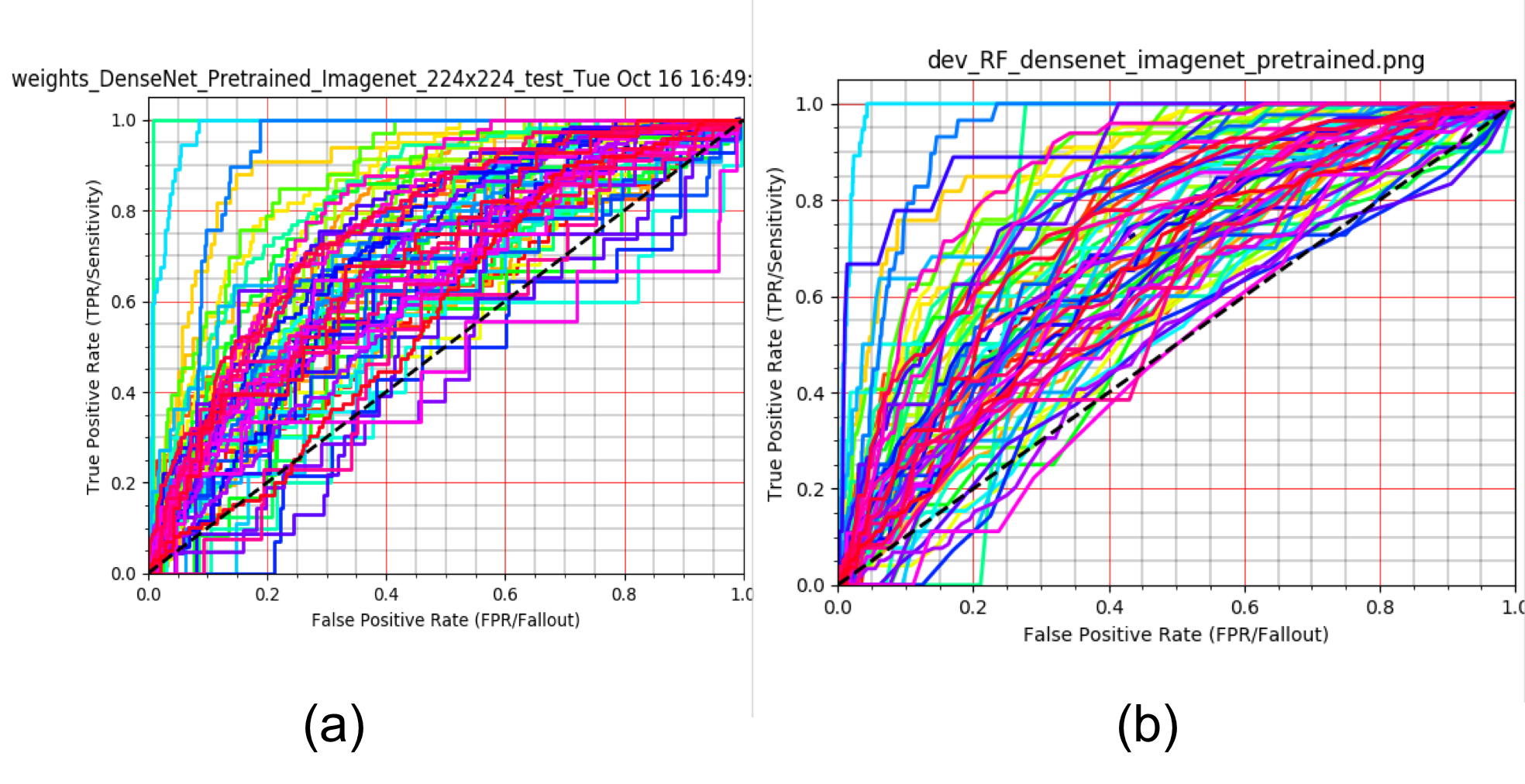
The experiments were performed with the newly labeled NIH dataset of 73 findings. A total of 7942 images were retained corresponding to the 73 labels that had support of at least 50 images in the collection. A total of 6209 images were used for training, and 1733 were retained for validation and testing. First, we generated a baseline result using DenseNet directly on the dataset. The predicted labels were then used to plot the ROC curves and area under curve (AUC) was noted. The resulting ROC curves and the average AUC are shown in Figure 6a. In the next experiment, we used the hybrid learning model of DenseNet feature generator with the random forest classifier. The resulting ROC curves are shown in Figure 6b using 5-fold cross-validation on a 80-20 split of training and test data. From this figure, we see that the performance of the two networks are similar although with more training epochs and data, it is likely that DenseNet would eventually outperform the hybrid classifier (both achieved an average AUC of 0.7). The list findings and the AUC for the second classifier are shown in Table 1 (only the first 32 are shown of the 73 derived labels). We can also observe from the results in Table 1 that the models in general perform better for higher level abstraction labels if the number of images for training are also larger. We conclude from these results that it is possible to train classifiers to recognize finer distinction labels of AP chest X-rays. However, the accuracy achieved still remains a function of the size of the labeled training datasets.

Fig. 6: Illustration of ROC curves for the 73 label dataset using (a) DenseNet (b) Deep ensemble classifier.

5 Conclusion

In this paper, we present a new chest X-ray benchmark database of 73 sentence-level findings seen in AP chest X-rays. We describe our method of obtaining these findings through a semi-automated ground truth generation process from crowdsourcing of clinical annotations.

References

- [1] Pranav Rajpurkar, Jeremy Irvin, Kaylie Zhu, Brandon Yang, Hershel Mehta, Tony Duan, Daisy Ding, Aarti Bagul, Curtis Langlotz, Katie Shpanskaya, et al., “Chexnet: Radiologist-level pneumonia detection on chest x-rays with deep learning,” arXiv preprint arXiv:1711.05225, 2017.
- [2] Xiaosong Wang, Yifan Peng, Le Lu, Zhiyong Lu, Mohammadhadi Bagheri, and Ronald M Summers, “Chestx-ray8: Hospital-scale chest x-ray database and benchmarks on weakly-supervised classification and localization of common thorax diseases,” in Computer Vision and Pattern Recognition (CVPR), 2017 IEEE Conference on. IEEE, 2017, pp. 3462–3471.
- [3] Jonathan Laserson, Christine Dan Lantsman, Michal Cohen-Sfady, Itamar Tamir, Eli Goz, Chen Brestel, Shir Bar, Maya Atar, and Eldad Elnekave, “Textray: Mining clinical reports to gain a broad understanding of chest x-rays,” arXiv preprint arXiv:1806.02121, 2018.
- [4] No Author, “Rsna pneumonia detection machine learning challenge now open,” http://www.rsna.org/News.aspx?id=24992, 2018.
- [5] Tanveer Syeda-Mahmood, Ritwik Kumar, and Colin Compas, “Learning the correlation between images and disease labels using ambiguous learning,” in International Conference on Medical Image Computing and Computer-Assisted Intervention. Springer, 2015, pp. 185–193.
- [6] Gao Huang, Zhuang Liu, Laurens Van Der Maaten, and Kilian Q Weinberger, “Densely connected convolutional networks.,” in CVPR, 2017, vol. 1, p. 3.
- [7] Jia Deng, Wei Dong, Richard Socher, Li-Jia Li, Kai Li, and Li Fei-Fei, “Imagenet: A large-scale hierarchical image database,” in Computer Vision and Pattern Recognition, 2009. CVPR 2009. IEEE Conference on. Ieee, 2009, pp. 248–255.
- [8] Chris Seiffert, Taghi M Khoshgoftaar, Jason Van Hulse, and Amri Napolitano, “Rusboost: A hybrid approach to alleviating class imbalance,” IEEE Transactions on Systems, Man, and Cybernetics-Part A: Systems and Humans, vol. 40, no. 1, pp. 185–197, 2010.
- [9] Joseph Sexton and Petter Laake, “Logitboost with errors-in-variables,” Computational Statistics & Data Analysis, vol. 52, no. 5, pp. 2549–2559, 2008.
- [10] Rong Yan, Jelena Tesic, and John R Smith, “Model-shared subspace boosting for multi-label classification,” in Proceedings of the 13th ACM SIGKDD international conference on Knowledge discovery and data mining. ACM, 2007, pp. 834–843.