The information geometry of 2-field functional integrals

Abstract

2-field functional integrals (2FFI) are an important class of solution methods for generating functions of dissipative processes, including discrete-state stochastic processes, dissipative dynamical systems, and decohering quantum densities. The stationary trajectories of these integrals describe a conserved current by Liouville’s theorem, despite the fact that there is no conserved phase space current in the underlying stochastic process. We develop the information geometry of generating functions for discrete-state classical stochastic processes in the Doi-Peliti 2FFI form, showing that the conserved current is a Fisher information between the underlying distribution of the process and the tilting weight of the generating function. To give an interpretation to the time invertibility implied by current conservation, we use generating functions to represent importance sampling protocols, and show that the conserved Fisher information is the differential of a sample volume under deformations of the nominal distribution and the likelihood ratio. We derive a new pair of dual Riemannian connections respecting the symplectic structure of transport along stationary rays that gives rise to Liouville’s theorem, and show that dual flatness in the affine coordinates of the coherent-state basis captures the special role played by coherent states in many 2FFI theories. The covariant convective derivative under time translation correctly represents the geometric invariants of generating functions under canonical transformations of the 2FFI field variables of integration.
Keywords: Information geometry; Doi-Peliti theory; Liouville’s theorem; Fisher information; importance sampling; duality

I Introduction: Understanding the Liouville theorems that emerge in 2-field functional integrals for dissipative systems

The defining feature of dissipative systems, whether classical or quantum, is that trajectories initially distinct can merge and that distributions or densities that differ at their initial conditions become more similar over time as they are increasingly governed by local generating parameters at the expense of memory. Because such systems are intrinsically irreversible, they obey no Liouville theorem (see Goldstein:ClassMech:01 ) describing phase space densities that are conserved along flow lines.

A powerful formalism for representing dissipative systems, both classical and quantum, is that of 2-field functional integrals (2FFI) that evolve the generating functions of distributions or densities. 2FFI methods with a shared integral form include the Doi-Peliti method for discrete-state processes Doi:SecQuant:76 ; Doi:RDQFT:76 ; Peliti:PIBD:85 ; Peliti:AAZero:86 , which will be used in this paper, the Martin-Siggia-Rose path integral for dynamical systems with Langevin noise Martin:MSR:73 , and the Schwinger-Keldysh time-loop formalism for quantum density matrices with decoherence Schwinger:MBQO:61 ; Keldysh:noneq_diag:65 . The modern approach traces back much further to a nonlinear action functional due to Onsager and Machlup Onsager:Machlup:53 for systems with Langevin noise, which can be derived from the 2-field formalism.

These integrals have the curious feature that their stationary-path analysis introduces a conserved volume element and Liouville theorem for just those systems that lack one in the state space. Conservation of a density along deterministic trajectories implies a form of temporal invertibility, and since this is not reversibility in the dynamical sense, it expresses a kind of time-duality. We are interested, then, in how such conserved densities are brought into existence by generating functions, and what is their meaning in terms of information.

In this paper we present the Liouville theorem and conserved volume element of 2FFI generating functions from an Information Geometry perspective Amari:inf_geom:01 ; Ay:info_geom:17 . To understand the concepts and questions that are unified under a geometric description, we give a brief synopsis of observations and claims that will be developed in the rest of the paper.

Synopsis of prior known facts and puzzles brought together and explained in this paper

Information geometry recognizes a duality with respect to the Fisher metric, between contravariant affine coordinates representing the intensity of a tilting weight in an exponential family such as the family of measures that define a generating function, and covariant coordinates which are the mean values in the resulting tilted distributions. Not surprisingly, those geometrically dual coordinates will be shown to coincide with the canonically conjugate coordinates evolving under the 2FFI Liouville theorem.

The concept of dual parallel transport that is central to information geometry arises naturally in 2FFI generating functions, coming from the same source as their time-duality. These integrals are constructed to propagate two measures through time on the same state space, one describing dynamical underlying distributions and the other the distribution of tilts that define a generating function from an exponential family over each underlying distribution. The independent freedom to vary these two measures leads to triples of distributions that, when compared under the generalized Pythagorean theorem Nagaoka:dual_geom:82 ; Amari:methods_IG:00 , define an inner product in the Fisher metric. The inner product has the interpretation of a sensitivity, or (more geometric) of a direction-cosine between vector fields associated with deformations in the base distribution and deformations in the tilt. Saddle-point or stationary-path conditions in the functional integral then define dual transport laws for the two measures under the action of a symplectic form, resulting in Liouville’s theorem.

To understand the meaning of densities conserved along stationary trajectories, we employ the interpretation of generating functions in terms of statistical inference and more specifically of Importance Sampling Owen:mcbook:13 . The tilt in a generating function becomes the likelihood ratio relating a nominal distribution to an importance distribution, and the conserved density of Liouville’s theorem becomes a differential volume element of sample probability. Dual transport of a conserved inner product in the Fisher metric, in turn, defines a transport law for the metric under coordinate transformations respecting the symplectic structure.

The use of dual Riemannian connections that is a cornerstone of information geometry provides a way to express dynamically meaningful features of a theory as geometric invariants under coordinate transformations. For 2FFI theories we construct a particular pair of dual connections, different from the dually flat connections introduced by Amari and Nagaoka Nagaoka:dual_geom:82 ; Amari:methods_IG:00 , to capture the following distinctive property of this class of theories:

Most introductions Mattis:RDQFT:98 ; Kamenev:DP:02 ; Baez:QTSM:17 of 2FFI methods derive them in bases of coherent states. These states correspond to mixture coordinates in the underlying distribution, and to the argument variables $z$ that are the tilting weights in a moment-generating function. They are contrasted to the cumulant-generating function arguments $\log z$ that are coordinates in the exponential family, and the mixture coordinate in the tilted (importance) distribution that are dual affine coordinates under the Amari-Nagaoka connections. The coherent state coordinates are not affine under the Fisher metric, and are not a basis for dualization through the Legendre transform, yet they are often the natural affine basis for the growth and contraction eigenvalues of the Liouville volume element on 2FFI stationary paths. The exponential and mixture families on the importance distribution are related to coherent states by a canonical transformation Smith:LDP_SEA:11 . We will show that dual connections describing flat parallel transport in coherent-state coordinates are the correct concept to capture the role of this basis in relation to the geometric role of coordinates in the exponential family. More generally, dual connections respecting the symplectic structure of translation along stationary rays define a covariant procedure for canonical transformation in 2-field integrals.

Organization of the presentation

The derivation of the these results is organized as follows: The first three sections review basic constructions that will be needed from information geometry (Sec. II), importance sampling (Sec. III), and the Doi-Peliti formalism for 2FFI generating functions (Sec. IV). The aim is to give a brief but self-contained introduction that will be understandable to readers from each area to whom the others may be unfamiliar, and to establish shared terms and notation. The dualities in information geometry and importance sampling apply to general families of probability distributions without reference to interpretations of time dependence, so they are presented first with emphasis on general coordinate transformations. The Doi-Peliti construction then brings in the additional features needed to evolve distributions under stochastic processes.

The main results of the paper are derived in Sec. V. It is shown that the conserved density that plays the role of a phase space density in Liouville’s theorem is a Wigner function on a product space that jointly evolves parameters associated with stochastic dynamics and with statistical inference. Deformations associated with underlying nominal distributions and with likelihood ratios are shown to define dual vector fields in the Fisher geometry on importance distributions, and their inner product corresponds to the differential volume element derived from the Wigner density. The transport law for the Fisher metric, and dual Riemannian connections respecting the symplectic structure, are then derived.

Sec. VI contains a simple worked example illustrating all aspects of the 2FFI Liouville theorem and its associated dual geometry. Sec. VII concludes, noting where the duality between dynamics and inference developed here extends and clarifies other studies of time-reversal duality that are currently active topics.

II The dual geometry from cumulant-generating functions for counts on integer lattices

Here we review the basic constructions of information geometry for generating functions over families of probability distributions indexed by some coordinate such as a first-moment value. No stochastic process or other notion of time dependence is assumed before Sec. IV. Rather than develop the generalized Pythagorean theorem in order to arrive at the projection theorem as originally done by Nagaoka and Amari Nagaoka:dual_geom:82 , we use the Pythagorean theorem to define an inner product between vector fields associated with independent variations in the family of underlying probability distributions and in the weights of their generating functions, which will be the main quantity conserved through time when time-dependence is introduced later. The condition for preservation of the inner product under coordinate transformations will be existence of a symplectic form, shown in later sections to be provided by the generators of time evolution in stochastic processes. The section retains as much as possible the notation of Amari:inf_geom:01 Ch. 6.

Scope of systems considered

Later results involving the symplectic geometry and Liouville theorem associated with 2-field functional integrals apply generally across discrete and continuous state spaces, for both classical and quantum (Schwinger-Keldysh time-loop) methods Kamenev:DP:02 . However, we will define geometric constructions only for probability distributions on discrete state spaces, as the simplest starting point to illustrate the idea.

For definiteness of notation, we will consider probability distributions on integer lattices in the positive orthant in ${\mathbb{Z}}^{D}$, appropriate to the description of population processes. Well-developed applications include evolutionary populations Smith:evo_games:15 and chemical reaction networks Krishnamurthy:CRN_moments:17 ; Smith:CRN_moments:17 . The dimensions in the lattice, indexed $i\in 1,\ldots,D$, define types in the population, which we will refer to as species; population states are vectors of integer-valued coefficients ${\rm n}\equiv\left({{\rm n}}_{i}\right)$, with ${{\rm n}}_{i}$ the count of species $i$; probability mass functions (which we will also refer to as probability distributions) are denoted ${\rho}_{{\rm n}}$.

II.1 The exponential families from generating functions for species counts

We will consider the simplest exponential families over a distribution ${\rho}_{{\rm n}}$, the linear families of generating functions for the species counts ${{\rm n}}_{i}$. Both moment-generating functions (MGF) and cumulant-generating functions (CGF) will be used. The ordinary power series MGF is a function of a vector of complex variables $z\equiv\left(z_{i}\right)$. The CGF is a function of the logarithms $\log z_{i}\equiv{\theta}^{i}$, which we introduce with a raised index to adopt the Einstein summation convention, that pairs of raised and lowered indices are summed. If $\theta$ and ${\rm n}$ are regarded as column vectors, ${\theta}^{T}$ stands for transpose. Compact notations for the vector $z$ raised component-wise to the power ${\rm n}$, and for the inner product of row and column vectors, are

$$z^{{\rm n}} \equiv\prod_{i=1}^{D}z_{i}^{{{\rm n}}_{i}}$$

$${\theta}^{T}{\rm n} \equiv{\theta}^{i}{{\rm n}}_{i}$$ (1)

In terms of these, the MGF denoted $\Psi$ and the CGF denoted $\psi$, are defined as

$$\Psi\!\left(z\right) \equiv\sum_{{\rm n}}z^{{\rm n}}{\rho}_{{\rm n}}$$

$$\equiv e^{\psi\left(\theta\right)} =\sum_{{\rm n}}{\rho}_{{\rm n}}e^{{\theta}^{T}{\rm n}}$$ (2)

$e^{{\theta}^{T}{\rm n}}$ is called an exponential tilt applied to the distribution ${\rho}_{{\rm n}}$. The normalized tilted distribution obtained by dividing by $e^{\psi\left(\theta\right)}$ is denoted

$${\tilde{\rho}}^{\left(\theta\right)}_{{\rm n}}\equiv{\rho}_{{\rm n}}e^{{\theta}^{T}{\rm n}-\psi\left(\theta\right)}$$ (3)

Normalization of ${\tilde{\rho}}^{\left(\theta\right)}_{{\rm n}}$ implies a value for the first moment, which we denote $n\!\left(\theta\right)$, of

$$n\!\left(\theta\right)\equiv{\left<{\rm n}\right>}_{{\tilde{\rho}}^{\left(\theta\right)}}=\frac{\partial\psi}{\partial\theta}$$ (4)

II.2 The Fisher metric on the exponential family of tilted distributions

II.2.1 The variance as local metric, and the Fisher distance element introduced

On a single underlying distribution ${\rho}_{{\rm n}}$, a small change of coordinate $\delta\theta$ in the exponential family leads to a change in the tilted distribution of

$$\delta\log{\tilde{\rho}}^{\left(\theta\right)}_{{\rm n}}=\delta{\theta}^{T}\left({\rm n}-n\!\left(\theta\right)\right)$$ (5)

The standard geometry on the exponential family of tilted distributions is introduced by using the variance under ${\tilde{\rho}}^{\left(\theta\right)}_{{\rm n}}$ to define a distance element between coordinates separated by a small increment $\delta\theta$ of

$$\delta s^{2} =\delta{\theta}^{i}\delta{\theta}^{j}\frac{{\partial}^{2}\psi\!\left(\theta\right)}{\partial{\theta}^{i}\partial{\theta}^{j}}$$

$$\equiv\delta{\theta}^{i}\delta{\theta}^{j}\sum_{{\rm n}}{\tilde{\rho}}_{{\rm n}}^{\left(\theta\right)}\left({{\rm n}}_{i}-n_{i}\!\left(\theta\right)\right)\left({{\rm n}}_{j}-n_{j}\!\left(\theta\right)\right)$$

$$\equiv\delta{\theta}^{i}\delta{\theta}^{j}g_{ij}\!\left(\theta\right)$$ (6)

$g\!\left(\theta\right)$, defined here as the Hessian of $\psi\!\left(\theta\right)$, is the Fisher metric tensor, introduced in this usage by Rao  Rao:info_metric:45 (reprinted as Rao:info_metric:92 ). Using the differential geometry notation in which ${\left\{\partial/\partial{\theta}^{i}\right\}}_{i=1}^{D}$ is the set of basis elements in the tangent space to the exponential family, the Fisher metric is an inner product, which we denote

$$g_{ij} \equiv\left<\frac{\partial}{\partial{\theta}^{i}},\frac{\partial}{\partial{\theta}^{j}}\right>$$ (7)

II.2.2 Coordinate dualization, Legendre transform, and the Large-Deviation function

Eq. (4) implies that the Fisher metric in Eq. (6) is a coordinate transformation from contravariant to covariant coordinates:

$$g_{ij}\!\left(\theta\right)=\frac{{\partial}^{2}\psi\!\left(\theta\right)}{\partial{\theta}^{i}\partial{\theta}^{j}}=\frac{\partial n_{i}\!\left(\theta\right)}{\partial{\theta}^{j}}$$ (8)

If $\psi\!\left(\theta\right)$ is convex, the transformation (8) is invertible. The inverse of the coordinate transform, and with it the Fisher metric, is obtained from the Legendre transform of $\psi\!\left(\theta\right)$,

$${\psi}^{\ast}\!\left(n\right)\equiv{\left[{\theta}^{T}n-\psi\!\left(\theta\right)\right]}_{\theta\left(n\right)}$$ (9)

where $\theta\left(n\right)$ is the maximizer of the argument in Eq. (9) over $\theta$ values. ${\psi}^{\ast}\!\left(n\right)$ is the Large-Deviation function (LDF), which will be used in Sec. III.

The Legendre transform is constructed to give

$$\frac{\partial{\psi}^{\ast}\!\left(n\right)}{\partial n_{i}}={\theta}^{i}\!\left(n\right)$$ (10)

so

$$\frac{\partial{\theta}^{i}}{\partial n_{j}}=\frac{{\partial}^{2}{\psi}^{\ast}\!\left(n\right)}{\partial n_{i}\partial n_{j}}\equiv g^{ij}\!\left(n\right)$$ (11)

the inverse of $g\!\left(\theta\right)$ from Eq. (8). It follows that the distance element (6) can be expressed in the dual covariant coordinates as

$$\delta s^{2}=\delta n_{i}\delta n_{j}g^{ij}\!\left(n\right)$$ (12)

The Fisher metric can be obtained as the projection of the Euclidean metric in ${\mathbb{R}}^{D}$ under a spherical embedding of the distribution ${\rho}_{{\rm n}}$, briefly reviewed in App. A.1, providing a third set of coordinates for the tilted distribution ${\tilde{\rho}}^{\left(\theta\right)}$. We note this embedding because it provides an interesting perspective on families of base distributions that are also exponential, which play several important roles in Doi-Peliti theory, and which we review next.

II.2.3 Exponential families on multinomial distributions

In general, the distribution ${\rho}_{{\rm n}}$ on which one wants to define an information geometry could have any structure, and could require arbitrarily much information to specify. An important sub-class of distributions, however, are those formed as products of Poisson marginal distributions over the independent counts ${{\rm n}}_{i}$, or sections through such products of marginals.

The Poisson

$${\rho}^{\left(n_{i}\right)}_{{{\rm n}}_{i}}=e^{-n_{i}}\frac{n_{i}^{{{\rm n}}_{i}}}{{{\rm n}}_{i}!}$$ (13)

is a minimum-information distribution; the expectations of its factorial moments Baez:QTRN_eq:14 , defined (again, component-wise) as ${{\rm n}}^{\underline{k}}\equiv{{\rm n}}!/{\left({\rm n}-k\right)}!$, are $n^{k}$ for all $k$. Products of Poisson marginals or multinomial distributions

$${\rho}^{\left(n\right)}_{{\rm n}}=\frac{1}{N^{N}}\left(\frac{N!}{{{\rm n}}_{1}!,\ldots,{{\rm n}}_{D}!}\right)\prod_{i=1}^{D}n_{i}^{{{\rm n}}_{i}}$$ (14)

arise as approximations to more complicated distributions in 2FFI stationary-point methods, and are also an important class of exact solutions for some applications such as chemical reaction network models Anderson:product_dist:10 . The stationary-point solutions in functional integrals are important whether or not they provide close approximations, as they define families of coordinate transformations that will be the basis to construct a dual symplectic geometry in Sec. V.

Distributions of the form (14) are both mixture families in the coordinates ${\left\{n_{i}\right\}}_{i=1}^{D}$, and exponential families in a suitable coordinate $\eta\propto\log n$ (introduced later in Sec. IV.4), which acts additively with the exponential coordinate $\theta$ of the CGF. A consequence of the simplification of the moment hierarchies in multinomial families is that the Fisher spherical embedding can be reduced to only $D$ dimensions in the coordinates $\left\{n_{i}/N\right\}$, where $N\equiv\sum_{j}n_{j}$, as reviewed in App. A.2. The reduction of functions of possibly-complicated distributions ${\rho}_{{\rm n}}$ such as Eq. (6) to functions of the same form involving only their coordinates $n_{i}$ arises repeatedly in the use of 2FFI stationary-point methods, so we note it in passing here.

II.3 The base and the tilt: inner products between vector fields describing two sources of variation

The most basic use of information geometries takes the distance element (6) as a point of departure to consider the geometry in the Fisher metric on a single exponential family of distributions ${\tilde{\rho}}^{\left(\theta\right)}_{{\rm n}}$, and develops the dual Riemannian connections on exponential coordinates $\theta$ and mixture coordinates $n$ that define parallel transport of ${\tilde{\rho}}^{\left(\theta\right)}_{{\rm n}}$ within that family. Here we wish to consider families of families, in which generating functions with coordinates $\theta$ are defined over families of distributions indexed by independent coordinates. Derivations of the Fisher metric from a divergence in that $2D$-dimensional family will define inner products between vectors in the two $D$-dimensional subspaces, to which we attach an interpretation in terms of statistical inference in Sec. III.

Therefore, in place of ${\rho}_{{\rm n}}$ in Eq. (2), let $\left\{{\rho}^{\left(n_{0}\right)}\right\}$ denote a family of distributions that we will call base distributions, where ${\rho}^{\left(n_{0}\right)}$ has first moment $n_{0}$. Over each base distribution define a family of CGFs and associated tilted distributions, denoted

$$e^{\psi\left(\theta,n_{0}\right)} \equiv\sum_{{\rm n}}{\rho}^{\left(n_{0}\right)}_{{\rm n}}e^{\theta\cdot{\rm n}}$$

$${\tilde{\rho}}^{\left(\theta,n_{0}\right)}_{{\rm n}} \equiv{\rho}^{\left(n_{0}\right)}_{{\rm n}}e^{\theta\cdot{\rm n}-\psi\left(\theta,n_{0}\right)}$$ (15)

The mixed change in $\psi\left(\theta,n_{0}\right)$ with two coordinates $\delta\theta$ in the tilt and $\delta n_{0}$ in the base, has an expression as a limit of the extended Pythagorean theorem Nagaoka:dual_geom:82 ; Amari:methods_IG:00 for Kullback-Leibler (KL) divergences which is also an inner product in the Fisher metric:

$$D\!\left({\tilde{\rho}}_{{\rm n}}^{\left(\theta,n_{0}+dn_{0}\right)}\,\right\rVert\left.{\tilde{\rho}}_{{\rm n}}^{\left(\theta,n_{0}\right)}\right)+D\!\left({\tilde{\rho}}_{{\rm n}}^{\left(\theta,n_{0}\right)}\,\right\rVert\left.{\tilde{\rho}}_{{\rm n}}^{\left(\theta+d\theta,n_{0}\right)}\right)$$

$$\mbox{}-D\!\left({\tilde{\rho}}_{{\rm n}}^{\left(\theta,n_{0}+dn_{0}\right)}\,\right\rVert\left.{\tilde{\rho}}_{{\rm n}}^{\left(\theta+d\theta,n_{0}\right)}\right)$$

$$=\sum_{{\rm n}}\left({\tilde{\rho}}_{{\rm n}}^{\left(\theta,n_{0}+dn_{0}\right)}-{\tilde{\rho}}_{{\rm n}}^{\left(\theta,n_{0}\right)}\right)\log\left(\frac{{\tilde{\rho}}_{{\rm n}}^{\left(\theta+d\theta,n_{0}\right)}}{{\tilde{\rho}}_{{\rm n}}^{\left(\theta,n_{0}\right)}}\right)$$

$$\rightarrow\delta{\theta}^{i}\delta n_{0j}\frac{{\partial}^{2}\psi\!\left(\theta,n_{0}\right)}{\partial{\theta}^{i}\partial n_{0j}}$$

$$\equiv\delta{\theta}^{i}\delta n_{0j}\left<\frac{\partial}{\partial{\theta}^{i}},\frac{\partial}{\partial n_{0j}}\right>$$ (16)

In the first equality of Eq. (16), $\delta\theta$ and $\delta n_{0}$ need not be small; this is the standard quantity used in the projection theorem defining a notion of orthogonality to an exponential family involving any three distributions separated from $\left(\theta,n_{0}\right)$ by $\delta\theta$ and $\delta n_{0}$. The second, limiting equivalence takes $\delta\theta\rightarrow 0$ and $\delta n_{0}\rightarrow 0$, to express differences of ${\tilde{\rho}}_{{\rm n}}$ and $\log{\tilde{\rho}}_{{\rm n}}$ in terms of the mixed second partial derivative of the KL divergence and hence the Fisher metric.

Recognizing that $\partial\psi/\partial{\theta}^{i}=n_{i}\!\left(\theta,n_{0}\right)$, the inner product in the final line of Eq. (16) is just the sensitivity

$$\left<\frac{\partial}{\partial{\theta}^{i}},\frac{\partial}{\partial n_{0j}}\right>=\frac{\partial n_{i}}{\partial{n_{0}}_{j}}$$ (17)

of the mean in the tilted distribution to variations in the base.

II.4 Preservation of the inner product in connection with Liouville’s theorem

A coordinate change from the mean in the base distribution to the mean in the tilted exponential distribution produces the metric in mixed coordinates that by construction is the Kronecker $\delta$:

$$\left<\frac{\partial}{\partial{\theta}^{i}},\frac{\partial}{\partial n_{j}}\right>={\delta}_{i}^{j}$$ (18)

and the coordinate inner product

$$\delta{\theta}^{i}\delta n_{0j}\left<\frac{\partial}{\partial{\theta}^{i}},\frac{\partial}{\partial n_{0j}}\right> \equiv\delta{\theta}^{i}\delta n_{i}$$ (19)

We may ask, for what one-parameter families of coordinate systems $\left(\theta\!\left(t\right),n\!\left(t\right)\right)$ is the coordinate inner product (18) conserved across the family? A one-parameter family of coordinates generates a one-parameter family of maps of vector fields $\delta\theta$ and $\delta n$ by the action

$${\left(\frac{d}{dt}\delta\theta\right)}^{i} =\delta{\theta}^{j}\frac{\partial}{\partial{\theta}^{j}}{\dot{\theta}}^{i}$$

$${\left(\frac{d}{dt}\delta n\right)}_{i} =\delta n_{j}\frac{\partial}{\partial n_{j}}{\dot{n}}_{i}$$ (20)

The condition

$$\frac{d}{dt}\left(\delta{\theta}^{i}\,\delta n_{i}\right)=0$$ (21)

will be met whenever

$$\frac{\partial{\dot{\theta}}^{i}}{\partial{\theta}^{j}}=-\frac{\partial{\dot{n}}_{j}}{\partial n_{i}}$$ (22)

where $\cdot$ denotes $d/dt$. Eq. (22) is satisfied if there is a symplectic form $\mathcal{L}\!\left(\theta,n\right)$ in terms of which the velocity vectors along trajectories can be written

$${\dot{\theta}}_{i} =\frac{\partial}{\partial n_{i}}\mathcal{L}\!\left(\theta,n\right)$$

$${\dot{n}}_{i} =-\frac{\partial}{\partial{\theta}_{i}}\mathcal{L}\!\left(\theta,n\right)$$ (23)

Alternatively, if Eq. (22) holds everywhere, the form $\mathcal{L}\!\left(\theta,n\right)$ can be constructed by integration.

Eq. (22) relates the dual contravariant and covariant coordinates under the Fisher metric as canonically conjugate variables in a Hamiltonian dynamical system. We return in Sec. IV to derive symplectic forms $\mathcal{L}\!\left(\theta,n\right)$ from the generators of stochastic processes, but first we note a sampling interpretation of the generating functions (2) that will provide intuition for the meaning of transporting an invariant inner product (18) along trajectories.

III Finite-system models as sample estimators; the Large-Deviation function, and importance sampling

Why develop an Importance Sampling interpretation of generating functions? – context from the wider applications of 2FFI duality

Looking ahead to Sec. IV, the 2-field structure in Doi-Peliti theory that we will describe geometrically in terms of dual connections and the Fisher metric reflects a natural duality that is present in the quadrature of any time-dependent stochastic process. The integral of the generator of time translations over any finite time interval allows expectations of random variables at a later time to be evaluated in measures derived by time evolution of probability distributions specified at earlier times. The evolution kernel that connects the two may be regarded either as a forward-time propagator of probability distributions or a reverse-time propagator of the random variables. The duality between these two interpretations of the time-evolution kernel was developed by Kolmogorov in his study of the “backward” generator or its (adjoint) “forward” generator Gardiner:stoch_meth:96 , and is the same as the equivalence of the Schrödinger picture (time evolution of states) and the Heisenberg picture (time evolution of operators) in quantum mechanics Cohen-Tannoudji:QM:77 .

A quite large literature has sprung up over the past 20 years making use of this forward/backward duality of time-dependent stochastic processes, focused on how path weights in time-dependent generating functionals may be used to exchange the roles of the generator and its adjoint. In that literature, when “physical interpretations” Seifert:stoch_thermo_rev:12 are assigned to backward propagation, the assignment is done in terms of time-reversal of physically traversed paths. Such an interpretation is inappropriate for the analysis we wish to provide of Liouville’s theorem and the symplectic structure of 2FFI constructions, on multiple grounds: i) it is needlessly restrictive: we wish to study stochastic processes in which paths together with their time-reverses may or may not be defined within the dynamics; ii) dynamical reversal is not fundamental to the Kolmogorov forward/backward duality: the sense in which the time-reversed propagation of random variables is “anti-causal” is inherent in the adjoint relation itself Smith:LDP_SEA:11 . Any mapping onto physical time-reversal depends on the strong and independent requirement that a system’s trajectory space contain an image of its own adjoint, which we do not generally wish to impose; iii) the physical time-reversal interpretation substitutes time-reversed for forward dynamics; to understand Liouville’s theorem in 2FFI theories, both maps under the forward generator and its adjoint must be co-present and meaningful.

It is in order to furnish an interpretation of the 2FFI symplectic transport structure, comparable to the phase-space density transport interpretation for Hamiltonian mechanics, that we appeal to statistical inference to assign informational meanings to the tilt weights used in generating functions. Beyond simply using the generating function as a mathematical device to extract moments from probability distributions, an importance sampling application gives the specific interpretation of a likelihood ratio to non-uniform as well as uniform weights as a transformation of measure for samples. It is then easy to understand how dual forward and backward generators can jointly propagate the images of regions in a probability distribution and regions of concentration or dilution under the likelihood ratio through time, and how densities of rays in these paired coordinates can reflect conserved information about the expectations of random variables in evolving distributions. This section notes the main steps in the importance-sampling interpretation.

III.1 States as samples; system scaling and sample aggregation

Statistical inference concerns the distributions and convergence properties of sample estimators for the parameters that define some underlying process, as a function of the scaling of samples under some aggregation rule.

There is no formal distinction between the ensemble output of a stochastic process as a model of the distribution of states taken by a finite-particle system on a discrete state space, and the output of the same process considered as a distribution of samples from the generating process. If sequences of states are modeled, the same equivalence holds for the stochastic process as a specifier of samples of trajectories.

The state of a system with multiple components defines a notion of the size of a sample from the generating process, and a rule for changing the number of components (e.g. the population size) defines an aggregation procedure over samples. The aggregation rule may correspond to simple repeated sampling from subsystems without replacement, or it may define a class of independent scaling behaviors, as the independent variation of different conserved quantities of the stoichiometry in a chemical reaction network does. The Laplace transform to the generating function, and its Legendre transform to the Large-Deviations Function, have direct interpretations in terms of sampling procedures and exponential scaling approximations in importance sampling.

III.2 Legendre transform and large deviations in the interpretation of importance sampling

In the terminology of importance sampling Owen:mcbook:13 , the base distribution ${\rho}^{\left(n_{0}\right)}$ corresponds to the nominal distribution, and the tilted (and normalized) distribution ${\tilde{\rho}}_{{\rm n}}^{\left(\theta,n_{0}\right)}$ of Eq. (15) plays the role of an importance distribution. The combined tilt and normalization $e^{{\theta}^{T}{\rm n}-\psi\left(\theta,n_{0}\right)}$ is the corresponding likelihood ratio, also called the Radon-Nikodym derivative of the measure between the base and the importance distributions.

Importance distributions ${\tilde{\rho}}^{\left(\theta,n_{0}\right)}$ can be chosen to concentrate the density of samples away from the mode of ${\rho}^{\left(n_{0}\right)}$ to values of ${\rm n}$ that are more informative about observables of interest. Tilts are typically chosen to minimize some cost function, such as the variance of samples. The large-deviation function can be derived as a leading exponential approximation to the tail weight of the base distribution, in a protocol tuned to minimize sample variance, as shown in the following construction from Siegmund:IS_seq_tests:76 .

To illustrate with an example in one dimension, an estimate of the probability that a particle count ${\rm n}$ exceeds some bound $\bar{n}$ can be obtained by sampling values of the random variable

$$h^{\left(\bar{n}\right)}_{{\rm n}}\equiv I\!\left\{{\rm n}>\bar{n}\right\}$$ (24)

the indicator function for ${\rm n}>\bar{n}$. In the base distribution ${\rho}^{\left(n_{0}\right)}$, the probability for ${\rm n}>\bar{n}$ is

$$P\!\left({\rm n}>\bar{n}\mid n_{0}\right)={\left<h^{\left(\bar{n}\right)}\right>}_{\left(n_{0}\right)}$$ (25)

An unbiased estimator for $P\!\left({\rm n}>\bar{n}\mid n_{0}\right)$ can be obtained by using the tilted distribution ${\tilde{\rho}}_{{\rm n}}^{\left(\theta,n_{0}\right)}$ of Eq. (15) and instead of accumulating the values $\left\{0,1\right\}$ of the indicator $h^{\left(\bar{n}\right)}$, accumulating values of the tilted observable

$${\tilde{h}}^{\left(\theta,\bar{n}\right)}_{{\rm n}} \equiv e^{\psi\left(\theta,n_{0}\right)-\theta{\rm n}}h_{{\rm n}}$$ (26)

The tilted estimator is unbiased because

$${\left<{\tilde{h}}^{\left(\theta,\bar{n}\right)}\right>}_{\left(\theta,n_{0}\right)}={\left<h^{\left(\bar{n}\right)}\right>}_{\left(n_{0}\right)}$$ (27)

A few lines of algebra, provided in App. B, show that an exponential bound for the estimator at any choices of $\theta$ and $\bar{n}$ is given by

$${\left<{\tilde{h}}^{\left(\theta,\bar{n}\right)}\right>}_{\left(\theta,n_{0}\right)} \leq e^{\psi\left(\theta,n_{0}\right)-\theta\bar{n}}$$ (28)

The variance of the same sample estimator has a corresponding bound (see Eq. (149))

$${\left<{\left({\tilde{h}}^{\left(\theta,\bar{n}\right)}\right)}^{2}\right>}_{\left(\theta,n_{0}\right)}-{\left<{\tilde{h}}^{\left(\theta,\bar{n}\right)}\right>}_{\left(\theta,n_{0}\right)}^{2}$$

$$\leq e^{\psi\left(\theta,n_{0}\right)-\theta\bar{n}}{\left<h^{\left(\bar{n}\right)}\right>}_{\left(n_{0}\right)}-{\left<h^{\left(\bar{n}\right)}\right>}_{\left(n_{0}\right)}^{2}$$ (29)

The parameter $\theta$ that minimizes the bound on sample variance (29) also gives the tightest bound (28) on the tail weight. It is the minimizing argument $\theta\!\left(\bar{n}\right)$ of Eq. (9), so the bound is given in terms of the LDF as.

$${\left<h^{\left(\bar{n}\right)}\right>}_{\left(n_{0}\right)} \leq e^{-{\psi}^{\ast}\left(\bar{n}\right)}$$ (30)

Without further assumptions about ${\rho}^{\left(n_{0}\right)}$ it is not possible to say more about the ratio ${\left<h^{\left(\bar{n}\right)}\right>}_{\left(n_{0}\right)}/e^{-{\psi}^{\ast}\left(\bar{n}\right)}$. The relevant additional property, which is also associated with the use and tightness of saddle-point approximations Goutis:saddlepts:95 in Doi-Peliti theory, is the onset of large-deviations scaling; that is, if $n_{0}$ and $\bar{n}$ are increased together in proportion to some scale factor $N$ as $\bar{n}=N\bar{\nu}$, $n_{0}=N{\nu}_{0}$, the following two limits should exist:

$$\lim_{N\rightarrow\infty}\frac{1}{N}{\psi}^{\ast}\!\left(N\bar{\nu}\right) ={\bar{\psi}}^{\ast}\!\left(\bar{\nu}\right)$$

$$\lim_{N\rightarrow\infty}\frac{1}{N}\psi\!\left(\theta\!\left(N\bar{\nu}\right);N{\nu}_{0}\right) =\bar{\psi}\!\left(\bar{\theta}\right)$$ (31)

Then the variance-minimizing tilt $\theta$ likewise has a limit, the variance ${\partial}^{2}\psi/\partial{\theta}^{i}\partial{\theta}^{j}$ in Eq. (6) scales as $N$, and the relative variance scales as $1/N$. App. B shows that in this limit the log ratio $\log\left[{\left<h^{\left(\bar{n}\right)}\right>}_{\left(n_{0}\right)}/e^{-{\psi}^{\ast}\left(\bar{n}\right)}\right]\leq\mathcal{O}\!\left(N^{1/2}\right)$, compared to ${\psi}^{\ast}\!\left(\bar{n}\right)\sim N$.

IV Doi-Peliti 2-field functional integrals, and dual mappings induced by time translation

A 2FFI formalism to compute time-dependent generating functions and functionals for stochastic processes with discrete state spaces has been developed based on the operator linear algebra for moment-generating functions due to Doi Doi:SecQuant:76 ; Doi:RDQFT:76 , and a coherent-state basis expansion due to Peliti Peliti:PIBD:85 ; Peliti:AAZero:86 that converts the Doi time-evolution operator into a functional integral. The Doi-Peliti method is now widely known Baez:QTSM:17 , so we will review here only definitions of essential terms and the detailed construction of the core elements, most importantly the coherent-state representation of the identity operator acting on generating functions. App. C provides some further supporting definitions and algebra. Self-contained introductory derivations following the notation used here are available in Smith:LDP_SEA:11 ; Smith:evo_games:15 ; Krishnamurthy:CRN_moments:17 ; Smith:CRN_moments:17 .

IV.1 Time evolution of moment- and cumulant-generating functions

The essential geometric constructions of Sec. II for tilted distributions, and the importance-sampling interpretation of Sec. III, are defined on distributions ${\rho}_{{\rm n}}$ without reference to any notion of embedding in a dynamical system. Here we add the feature of a continuous-time master equation

$$\frac{d{\rho}_{{\rm n}}}{dt} =\sum_{{{\rm n}}^{\prime}}{\rm T}_{{\rm n}{{\rm n}}^{\prime}}{\rho}_{{{\rm n}}^{\prime}}.$$ (32)

that evolves densities ${\rho}_{{\rm n}}$ along a coordinate $t$. In physical applications $t$ is time, but for the purpose of this paper, $t$ may be any one-dimensional coordinate along which we can define a continuous mapping of probability distributions, or even just a continuous family of coordinate transformations in which to describe the geometry of a single distribution regarded as fixed. ${\rm T}_{{\rm n}{{\rm n}}^{\prime}}$ is known as the transition matrix, and is the representation of the generator of the stochastic process acting in the space of probability distributions. It is left-stochastic, meaning $\sum_{{\rm n}}{\rm T}_{{\rm n}{{\rm n}}^{\prime}}=1$, $\forall{{\rm n}}^{\prime}$, ensuring conservation of probability. The matrix elements ${\rm T}_{{\rm n}{{\rm n}}^{\prime}}$ can depend on the time $t$, though in the example developed in Sec. VI we will use a time-independent generator for simplicity.

IV.1.1 Laplace transform converts that master equation on distributions to a Liouville equation on moment-generating functions

The Doi-Peliti method works not with the distribution ${\rho}_{{\rm n}}$ in the discrete basis, but with the moment-generating function (2) that is its Laplace transform. From the form of the transition matrix ${\rm T}_{{\rm n}{{\rm n}}^{\prime}}$ it is possible to derive a Liouville equation (see any of Smith:LDP_SEA:11 ; Smith:evo_games:15 ; Krishnamurthy:CRN_moments:17 ; Smith:CRN_moments:17 ) for the time-dependence of the MGF,

$$\frac{\partial}{\partial t}\Psi\!\left(z\right) =-\mathcal{L}\!\left(z,\frac{\partial}{\partial z}\right)\Psi\!\left(z\right),$$ (33)

$\mathcal{L}\!\left(z,\partial/\partial z\right)$, called the Liouville operator, is the representation of the generator of the stochastic process acting in the space of generating functions, and is conventionally defined with the minus sign of Eq. (33) because its spectrum is non-negative. The Liouville operator will play the role of a Hamiltonian as a generator of symplectomorphisms in the derivation below.

IV.1.2 The Doi operator representation of the Hilbert space of generating functions

For many purposes, the properties of the generating function as an analytic function of a complex variable are not needed, and the algebra of the MFG as a formal power series is sufficient. To capture only this algebra, in a notation that is more convenient than that of analytic functions for computing the quadrature of Eq. (33), the Doi formalism Doi:SecQuant:76 ; Doi:RDQFT:76 replaces the variable $z$ and derivative $\partial/\partial z$ with formal raising and lowering operators

$$z_{i} \rightarrow a^{\dagger}_{i}; \frac{\partial}{\partial z_{i}} \rightarrow a^{i}$$ (34)

as are conventionally used in quantum mechanics or quantum field theory Baez:QTSM:17 . In the condensed notation (2) for vector inner products, we will regard $a$ as a column vector and $a^{\dagger}$ as a row vector.

Associated with operators $a^{\dagger}_{i}$ and $a^{i}$ are bilinear number operators ${\hat{n}}_{i}\equiv a^{\dagger}_{i}a^{i}$ (no Einstein sum), of which the basis monomials $z^{{\rm n}}$ under the mapping (34) correspond to number eigenstates. A Hilbert space of generating functions, and an inner product corresponding to the evaluation of the MGF at argument $z=1$, are defined and given a standard bracket notation reviewed in App. C. Number states are denoted $\left|{\rm n}\right)$, and the MGF $\Psi\!\left(z\right)$ is represented as a state vector $\left|\Psi\right)$ defined in terms of number states as

$$\sum_{{\rm n}}{\rho}_{{\rm n}}\left|{\rm n}\right)\equiv\left|\Psi\right)$$ (35)

The Liouville equation (33) becomes

$$\frac{d}{dt}\left|\Psi\right) =-\mathcal{L}\!\left(a^{\dagger},a\right)\left|\Psi\right).$$ (36)

in which the the Liouville operator $\mathcal{L}\!\left(a^{\dagger},a\right)$ is the former function $\mathcal{L}\!\left(z,\partial/\partial z\right)$ under the substitution (34).

The analytic form (2) of the MGF can be recovered using a variant of the Glauber norm that defines the inner product on the Hilbert space, as

$$\left(0\right|e^{za}\left|\Psi\right)=\Psi\!\left(z\right).$$ (37)

In Eq. (37), $z$, like $a^{\dagger}$, is regarded as a row vector and $za$ is the scalar product of $z$ and $a$. We will need the analytic form to relate the Doi-Peliti functional integral to the coordinates $\theta$ in which the geometry of Sec. II has been constructed.

IV.2 The 2FFI representation of the identity on distributions

IV.2.1 Coherent states and the Peliti construction of the functional integral

The objective in introducing the Doi operator formalism is to more conveniently compute the quadrature of the Liouville equation (33), formally written

$${\left|\Psi\right)}_{T} =\mathcal{T}e^{-\int_{0}^{T}dt\mathcal{L}\left(a^{\dagger},a\right)}{\left|\Psi\right)}_{0}$$

$$\equiv\lim_{\delta t\rightarrow 0}\mathcal{T}\prod_{k=1}^{T/\delta t}e^{-\delta t{\mathcal{L}\left(a^{\dagger},a\right)}_{k\delta t}}{\left|\Psi\right)}_{0}$$ (38)

${\left|\Psi\right)}_{T}$ is the generating function for the distribution ${\rho}_{{\rm n}}$ evolved to time $t=T$ from the generating function ${\left|\Psi\right)}_{0}$ for an initial distribution given at time $t=0$. $\mathcal{T}$ denotes time-ordering of the exponential integral, defined operationally in the second line of Eq. (38), in terms of a time-ordered product of applications of $\mathcal{L}\!\left(a^{\dagger},a\right)$ evaluated at the sequence of times $k\delta t$.

The 2FFI method of solution due to Peliti Peliti:PIBD:85 ; Peliti:AAZero:86 makes use of the coherent states as a basis for the expansion of arbitrary generating functions. Coherent states, defined in terms of a (column) vector $\phi$ of complex coefficients by

$$\left|\phi\right) \equiv e^{\left(a^{\dagger}-1\right)\phi}\left|0\right)$$ (39)

are the generating functions of products of Poisson distributions with component-wise mean values ${\phi}^{i}$, and eigenstates of the lowering operator:

$$a^{i}\left|\phi\right)={\phi}^{i}\left|\phi\right)$$ (40)

An essential feature of the of the Doi Hilbert space and inner product, explained in App. C, is that dual to each basis basis vector in the number basis (corresponding to the monomials $z^{{\rm n}}$) is a projection operator extracting the amplitude with which that state appears in $\left|\Psi\right)$. For the number basis these are just the probability values ${\rho}_{{\rm n}}$. In the same manner, dual to coherent states there are projection operators defined in terms of (row) vectors ${\phi}^{\dagger}$ of complex coefficients that are the complex conjugates of the components of $\phi$. Using the normalization consistent with Eq. (39) for $\left|\phi\right)$ the dual projectors are defined as

$$\left(\phi\right| \equiv e^{\left(1-{\phi}^{\dagger}\right)\phi}\left(0\right|e^{{\phi}^{\dagger}a}.$$ (41)

Unlike the number states and their dual projectors, which are complete, the coherent states and their dual projectors are over-complete. The inner product of a state at parameter ${\phi}_{1}$ with a projector at parameter ${\phi}^{\dagger}_{2}$ is given by

$$\left({\phi}^{\dagger}_{2}\,\right|\!\left.\vphantom{{\phi}^{\dagger}_{2}}{\phi}_{1}\right) =e^{-{\phi}^{\dagger}_{2}\left({\phi}_{2}-{\phi}_{1}\right)}$$ (42)

The inner product (42) is very important because it is the source of a “kinetic term” analogous to $p\dot{q}$ in classical Hamiltonian mechanics that causes the Liouville operator to behave as a Hamiltonian in the Doi-Peliti field theory.

Although they are overcomplete, the coherent states and their dual projectors furnish a representation of the identity in the space of generating functions, as shown in App. C.2,

$$\int\frac{d^{D}\!{\phi}^{\dagger}d^{D}\!\phi}{{\pi}^{D}}\left|\phi\right)\left(\phi\right| =I$$ (43)

When a copy of the identity (43) is inserted into the quadrature (38) between each increment of evolution of length $\delta t$, and the generating function is evaluated at argument $z$ using the inner product (37), the resulting MGF or CGF of Eq. (2) can be written as the functional integral

$$e^{{\psi}_{T}\left(\theta\right)}=\int_{0}^{T}{\mathcal{D}}^{D}\!{\phi}^{\dagger}{\mathcal{D}}^{D}\!{\phi}\,e^{\left(z-{\phi}^{\dagger}_{T}\right){\phi}_{T}-S+{\psi}_{0}\left(\log{\phi}^{\dagger}_{0}\right)}$$ (44)

$e^{{\psi}_{0}\left(\log{\phi}^{\dagger}_{0}\right)}$ is the coherent-state expansion of the initial generating function ${\left|\Phi\right)}_{0}$ in Eq. (38). $S$ in Eq. (44) has the form of a Lagrange-Hamilton action functional,

$$S =\int_{0}^{T}dt\left\{-\left(d_{t}{\phi}^{\dagger}\right)\phi+\mathcal{L}\!\left({\phi}^{\dagger},\phi\right)\right\}$$ (45)

in which the kinetic term comes from the log of the inner product (42) in the continuous-time limit, and the Liouville operator $\mathcal{L}\!\left({\phi}^{\dagger},\phi\right)$, with ${\phi}^{\dagger}$ and $\phi$ replacing operators $a^{\dagger}$ and $a$, playing the role of the Hamiltonian. The action (45) will be the source of the relation (23) leading to a conserved volume element and Liouville theorem in the information geometry for dissipative stochastic processes.

IV.2.2 The Peliti functional integral as a statistical model

The Peliti basis of coherent states (39) defines a statistical model for the stochastic process. The role of the projection operators in the representation of unity (43) in populating the model can be clarified by splitting the functional integral (45) at any intermediate time $t$, in the same fashion as the Chapman-Kolmogorov equation splits the time evolution of a probability distribution by a sum over intermediate states. This is done by integrating Eq. (44) up to time $t$, inserting an explicit representation of unity in terms of a pair of fields $\left({\phi}_{\ddagger}^{\dagger},{\phi}_{\ddagger}\right)$, and resuming the functional integral on the generating function extracted by that representation of unity:

$$e^{{\psi}_{T}\left(\theta\right)}=\int_{t+\delta t}^{T}{\mathcal{D}}^{D}\!{\phi}^{\dagger}{\mathcal{D}}^{D}\!{\phi}\,e^{\left(z-{\phi}^{\dagger}_{T}\right){\phi}_{T}-S}\int d^{D}\!{\phi}_{\ddagger}e^{\left({\phi}^{\dagger}_{t+\delta t}-1\right){\phi}_{\ddagger}}\int\frac{d^{D}\!{\phi}^{\dagger}_{\ddagger}}{{\pi}^{D}}e^{-\left({\phi}^{\dagger}_{\ddagger}-1\right){\phi}_{\ddagger}}e^{{\psi}_{t}\left(\log{\phi}^{\dagger}_{\ddagger}\right)}$$ (46)

In Eq. (46) the argument $\log{\phi}^{\dagger}_{\ddagger}$ is an affine tilt coordinate in an exponential family of generating functions on whatever base distribution the functional integral produces at time $t$. The (component-wise) product ${\phi}^{\dagger}_{t+dt}{\phi}_{\ddagger}$ (see also Sec. IV.4.1 below) is a dual mixture coordinate, corresponding to the mean of $n$ in the importance distribution with $\left|{\phi}_{\ddagger}\right)$ as the base distribution and ${\phi}^{\dagger}_{t+dt}$ as the likelihood ratio. It is the mean of this importance distribution, together with the log-likelihood that is its dual coordinate in the exponential family, that must transform under symplectomorphism to satisfy the condition (23) for preservation of inner products. The next section shows that the stationary-path conditions provide the necessary mapping.

IV.3 Stationary paths of the 2-field action functional

A deterministic approximation to the mean values through time in the base distribution, and to the mean weights in the likelihood ratio, is given by the saddle point of $e^{-S}$ in Eq. (44). The functional has a saddle point where the variational derivative of $S$ vanishes, leading to the stationary-path equations of motion

$${\dot{\phi}^{\dagger}}_{i} =\frac{\partial}{\partial{\phi}_{i}}\mathcal{L}\!\left({\phi}^{\dagger},\phi\right)$$

$${\dot{\phi}}_{i} =-\frac{\partial}{\partial{\phi}^{\dagger}_{i}}\mathcal{L}\!\left({\phi}^{\dagger},\phi\right)$$ (47)

which are of Hamiltonian form.

The final-time boundary value for the field ${\phi}^{\dagger}$ is given by the vanishing derivative of the exponent in Eq. (44) with respect to ${\phi}_{T}$, resulting in ${\phi}^{\dagger}_{T}=z$. The initial time boundary value for $\phi$ is given, after an integration by parts, by the vanishing derivative with respect to ${\phi}^{\dagger}_{0}$, and depends on the form of the CGF ${\psi}_{0}$ and the stationary-path value of its argument ${\phi}^{\dagger}_{0}$. The two conditions are solved self-consistently through the equations (47).

As the discussion following Eq. (46) highlights, joint stationary values at intermediate times $t$, in a generating function with argument $z$ imposed at a final time $T$, represent the bundle of rays in the statistical model that dominate the contribution to the importance distribution at later times. For this reason the stationary trajectory in the base distribution is not generally independent of the trajectory for the tilt in systems with non-linear equations of motion. The ray interpretation is well developed in Freidlin-Wentzell theory Freidlin:RPDS:98 for eikonal approximations to boundary-value problems for diffusion equations, and with respect to 2FFI solutions for first-passage times and escape trajectories Maier:escape:93 ; Maier:scaling:96 ; Maier:oscill:96 ; Maier:exit_dist:97 .

Our use of the stationary-path equations (47) will be to define a 1-parameter family of coordinate transformations in the manifold of coordinates for base distributions and likelihood functions. These may be viewed as dynamical maps of distributions through time, or they may simply be used as alternative coordinate systems in which to evaluate inner products of vector fields on a fixed distribution.

IV.4 Canonical transformations of the field variables of integration

An important class of changes of variable in 2-field integrals are those corresponding to the canonical transformations in Hamiltonian mechanics Goldstein:ClassMech:01 . The canonical transformations preserve the form of the kinetic term in the action (45), and thus the separation into conjugate field pairs with a preserved volume element. Three canonical transformations are heavily used in 2FFI generating functions, and each of them plays a role in our construction of a dual symplectic geometry.

IV.4.1 An action-angle transform from coherent-state variables to number-potential variables

A transformation from coherent-state fields to what would be “action-angle” variables in classical mechanics is defined by

$${\phi}_{i}^{\dagger} \equiv e^{{\theta}^{i}} {\phi}_{i} \equiv e^{-{\theta}^{i}}n_{i}$$ (48)

$n$, corresponding to the bilinear ${\phi}^{\dagger}\phi$ has the interpretation of the number coordinate in the importance distribution, and its conjugate $\theta$ has the interpretation of a potential, such as the chemical potential in a chemical-reaction application Smith:LDP_SEA:11 ; Krishnamurthy:CRN_moments:17 ; Smith:CRN_moments:17 . $\theta$ also corresponds directly to the coordinate $\log z$ which is the affine coordinate in the exponential family of tilted distributions (3). $n$ and $\theta$ are thus dual mixture and exponential coordinates with respect to the Fisher geometry Amari:inf_geom:01 ; Ay:info_geom:17 .

The action (45) in action-angle variables becomes

$$S =\int_{0}^{T}dt\left\{-\left(d_{t}\theta\right)n+\mathcal{L}\!\left(\theta,n\right)\right\}$$ (49)

$\mathcal{L}\!\left(\theta,n\right)$ is $\mathcal{L}\!\left({\phi}^{\dagger},\phi\right)$ with ${\phi}^{\dagger}$ and $\phi$ written as functions of $n$ and $\theta$ by Eq. (48). The stationary-path equations corresponding to Eq. (47) in action-angle variables are

$${\dot{\theta}}_{i} =\frac{\partial}{\partial n_{i}}\mathcal{L}\!\left(\theta,n\right)$$

$${\dot{n}}_{i} =-\frac{\partial}{\partial{\theta}_{i}}\mathcal{L}\!\left(\theta,n\right)$$ (50)

IV.4.2 Descaling with respect to the instantaneous steady-state mean number

A second class of canonical transformations, performed by transferring a scale factor from $\phi$ to ${\phi}^{\dagger}$, was first used in Doi-Peliti integrals by Baish Baish:DP_duality:15 . Let ${\bm{n}}$ be the saddle-point value of the field $n$ in Eq. (48) in the steady state that would be annihilated by ${\rm T}_{{\rm n}{{\rm n}}^{\prime}}$ at the parameters it possesses at some time. If ${\rm T}_{{\rm n}{{\rm n}}^{\prime}}$ and thus $\mathcal{L}$ is explicitly time-dependent, then the scale factor ${\bm{n}}$ will generally be different for each time. Define coherent state fields rescaled locally by ${\bm{n}}$ as

$${\phi}^{\dagger}_{i}{\bm{n}}_{i} \equiv{\varphi}^{\dagger}_{i} \frac{{\phi}_{i}}{{\bm{n}}_{i}} \equiv{\varphi}_{i}$$ (51)

The form of the action in fields $\left({\varphi}^{\dagger},\varphi\right)$ remains as in Eq. (45) but the Liouville function $\mathcal{L}$ which was the “Hamiltonian” for the stationary-path equations (47) is replaced by a possibly-shifted function

$$\mathcal{\tilde{L}}\!\left({\varphi}^{\dagger},\varphi\right)\equiv\mathcal{L}\!\left({\phi}^{\dagger},\phi\right)+\sum_{i}\left({\varphi}^{\dagger}_{i}{\varphi}^{i}\right)d_{t}\log{\bm{n}}_{i}$$ (52)

Canonical transformation by coherent-state rescaling is closely related to a class of similarity transforms of the transition matrix introduced by Hatano and Sasa Hatano:NESS_Langevin:01 , and now widely used as the basis for a class of integral fluctuation theorems Verley:HS_FDT:12 . The Hatano-Sasa dualization and the Baish dualization differ in the important respect that Hatano and Sasa rescale the entire transition matrix ${\rm T}_{{\rm n}{{\rm n}}^{\prime}}$ by values of the stationary probability density ${\rho}_{{\rm n}}$, requiring knowledge of infinitely many scale factors, whereas the rescaling (51) requires only $D$ scale factors (the stationary-point numbers of the $D$ species ${\bm{n}}_{i}$). The two coincide exactly in the case that the distribution is a coherent state, for which all probability values are expressed in terms of the mean. This is just the case in which the Fisher spherical embedding of a general probability distribution, reviewed in App. A.1, projects to a spherical embedding of the same form in terms of only the mean number, as shown in App. A.2.

Dual action-angle transform in descaled coherent states

An instance of the action-angle transformation that we have not seen used before, but which directly gives the dual geometry for the symplectic structure of Liouville evolution, is one applied to the rescaled coherent-state fields $\left({\varphi}^{\dagger}.\varphi\right)$:

$${\varphi}^{\dagger}_{i} \equiv e^{-{\eta}_{i}}n_{i} {\varphi}_{i} \equiv e^{{\eta}_{i}}$$ (53)

The action (45) in the new variables becomes

$$S=\int_{0}^{T}dt\left\{\left(d_{t}\eta\right)n+\mathcal{\tilde{L}}\!\left(n,\eta\right)\right\}$$ (54)

where the modified Liouville function $\mathcal{\tilde{L}}$ from Eq. (52) must be used, such that in the new variables

$$\mathcal{\tilde{L}}\!\left(n,\eta\right)\equiv\mathcal{L}\!\left(\theta,n\right)+\sum_{i=1}^{D}n_{i}d_{t}\log{\bm{n}}_{i}$$ (55)

$\eta$ is the affine coordinate in an exponential family of distributions produced by tilting a reference which is a product of Poisson marginals, or an equivalent section through that product, such as a multinomial.

IV.4.3 Time-translation along stationary paths

The third class of canonical transformations are the coordinate transformations generated by time-translation along stationary paths. For any coordinate system $\left(\theta,n\right)$, the bundle of stationary trajectories $\left(\bar{\theta},\bar{n}\right)$ passing through those values at a time $t$, together with a time-shift $\Delta t$, generate new coordinates

$$\left({\theta}^{\prime},n^{\prime}\right)\equiv{\left.\left(\bar{\theta}\!\left(t+\Delta t\right),\bar{n}\!\left(t+\Delta t\right)\right)\right|}_{\left(\bar{\theta}\left(t\right),\bar{n}\left(t\right)\right)=\left(\theta,n\right)}$$ (56)

which also obey Eq. (50), possibly with shifted parameters in $\mathcal{L}$.

We will be interested in the class of dual Riemannian connections that can be imposed on 2-field coordinate systems that respect the symplectic structure of the generator $d/dt$ of canonical transformations by time translation.

V The Liouville theorem connecting dynamics to inference induced by 2-field stationary trajectories

Liouville’s theorem in classical mechanics describes conservation of a phase space density over position coordinates and their conjugate momenta. The discrete-state stochastic processes for which Doi-Peliti methods were invented do not possess conjugate momentum coordinates, and their measures over positions concentrate as trajectories coalesce. For other groups of 2FFI methods such as Martin-Siggia-Rose Martin:MSR:73 , although the states may be those of dynamical systems, the dissipative context for which these methods are applied likewise do not conserve density in the resulting phase spaces. Instead, the 2-field integrals themselves provide fields that relate to the coherent-state parameters as conjugate momenta under the Liouville function $\mathcal{L}$, which admit (among other possibilities) the interpretation of likelihood ratios.

This section constructs the conserved density in a 2FFI-“phase space” in which the conjugate coordinates represent forward-propagating nominal distributions and backward-propagating likelihoods with the interpretation of sampling protocols for inference. The conserved density is only the scalar representation of symplectic structure; the deformations in the Liouville volume element carried on stationary paths imply further transport laws for vector and tensor fields including the Fisher metric. Those are derived next by writing the inner product of vector fields from base and tilt variations as the basis for the $2D$-dimensional differential of the CGF.

V.1 The Wigner function from the 2-field identity operator plays the role of a phase-space density

The scalar density in 2FFI that fills the role of a phase space density in classical Hamiltonian mechanics is the Wigner function Wigner:quantum_density:35 , of which versions exist for both classical and quantum systems. It is defined in terms of the representation of unity in Eq. (46), as

$$w_{t}\!\left({\phi}^{\dagger}_{\ddagger},{\phi}_{\ddagger}\right) \equiv\frac{1}{{\pi}^{D}}\int_{t+\delta t}^{T}{\mathcal{D}}^{D}\!{\phi}^{\dagger}{\mathcal{D}}^{D}\!{\phi}\,e^{\left(z-{\phi}^{\dagger}_{T}\right){\phi}_{T}-S}e^{\left({\phi}^{\dagger}_{t+\delta t}-{\phi}^{\dagger}_{\ddagger}\right){\phi}_{\ddagger}}e^{{\psi}_{t}\left(\log{\phi}^{\dagger}_{\ddagger}\right)}$$ (57)

Eq. (57) implies that, for $w_{t}\!\left({\phi}^{\dagger}_{\ddagger},{\phi}_{\ddagger}\right)$ at any time,

$$e^{{\psi}_{T}\left(\theta\right)}=\int d^{D}\!{\phi}^{\dagger}_{\ddagger}\,d^{D}\!{\phi}_{\ddagger}\,w_{t}\!\left({\phi}^{\dagger}_{\ddagger},{\phi}_{\ddagger}\right)$$ (58)

In a saddle-point approximation, one identifies arguments $\left({\bar{\phi}}^{\dagger}_{\ddagger},{\bar{\phi}}_{\ddagger}\right)$ for which, to leading exponential order,

$$e^{{\psi}_{T}\left(\theta\right)}\sim w_{t}\!\left({\bar{\phi}}^{\dagger}_{\ddagger},{\bar{\phi}}_{\ddagger}\right)$$ (59)

Since Eq. (59) approximates the same function at any time $t$, its total time derivative along the sequence of stationary points must vanish,

$$0 =\frac{d}{dt}w_{t}\!\left({\bar{\phi}}^{\dagger}_{\ddagger},{\bar{\phi}}_{\ddagger}\right)$$

$$=\left(\frac{\partial}{\partial t}+\frac{d{\bar{\phi}}^{\dagger}_{\ddagger}}{dt}\frac{\partial}{\partial{\bar{\phi}}^{\dagger}_{\ddagger}}+\frac{d{\bar{\phi}}_{\ddagger}}{dt}\frac{\partial}{\partial{\bar{\phi}}_{\ddagger}}\right)w_{t}\!\left({\bar{\phi}}^{\dagger}_{\ddagger},{\bar{\phi}}_{\ddagger}\right)$$ (60)

Moreover, the stationary points should coincide with values along the stationary trajectories (47) of the functional integral (46), which satasify

$${\left.\left(\sum_{i}\frac{\partial{\dot{\phi}}^{\dagger}_{i}}{\partial{\phi}^{\dagger}_{i}}+\sum_{i}\frac{\partial{\dot{\phi}}_{i}}{\partial{\phi}_{i}}\right)\right|}_{{\bar{\phi}}^{\dagger},\bar{\phi}}=0$$ (61)

Eq. (60) may thus be recast as the conservation law for a $2D$-dimensional current $\left({\dot{\phi}}^{\dagger}w,{\dot{\phi}}w\right)$,

$$0=\frac{\partial w_{t}}{\partial t}+\sum_{i}\frac{\partial}{\partial{\phi}^{\dagger}_{i}}\left({\dot{\phi}}^{\dagger}_{i}w_{t}\right)+\sum_{i}\frac{\partial}{\partial{\phi}_{i}}\left({\dot{\phi}}_{i}w_{t}\right)$$ (62)

which is Liouville’s theorem.

$w_{t}$ is a density of rays for joint base distributions and likelihood ratios that is conserved along the Doi-Peliti stationary trajectories. $\log w_{t}$ is the leading exponential approximation to the value of the CGF. It therefore integrates information along the trajectory from the final-time imposed value of $z$ and the initial-time structure of the generating function ${\psi}_{0}\!\left(\log{\phi}^{\dagger}_{0}\right)$.

The indirect definition (57) of the Wigner function in terms of the functional integral is convenient to manipulate but perhaps not very self-explanatory. App. D gives a direct construction of the stationary-point approximation in terms of a density $\rho\!\left(\theta\right)$ over the basis of coherent states $\left|\phi\right)$ and their Laplace transforms, and verifies that the sequence of stationary points do indeed coincide with the equations of motion (47).

Constraints and conserved current flows in reduced dimensions

Often systems of interest will evolve under constraints arising from conservation laws, such as conserved quantities of the stoichiometry in chemical reaction networks Polettini:open_CNs_I:14 ; Krishnamurthy:CRN_moments:17 ; Smith:CRN_moments:17 . Conserved quantities result in flat directions in the CGF and zero eigenvalues of the Fisher metric. Since generally the constraints will involve multiple species, and because the action-angle canonical transform (48) is defined in the species basis, it will not be possible to factor out non-dynamical combinations. Then the transport equation (62) for the current of the Wigner density will occupy only a sub-manifold of the $2D$-dimensional Doi-Peliti coordinate space needed to define the system.

A convenient way to handle constraints is to work in the eigenbasis of the Fisher metric which we will index with subscript $\alpha$, where an action-angle counterpart to the transport equation (62) reads

$$0 =\frac{\partial w_{t}}{\partial t}+\sum_{\alpha}\frac{\partial}{\partial{\theta}^{\alpha}}\left({\dot{\theta}}^{\alpha}w_{t}\right)+\sum_{\alpha}\frac{\partial}{\partial n_{\alpha}}\left({\dot{n}}_{\alpha}w_{t}\right)$$ (63)

The picture of the Liouville equation as implying a conserved volume element

$$\frac{d}{dt}\left(\prod_{\alpha}\delta{\theta}^{\alpha}\delta n_{\alpha}\right)=0$$ (64)

with the product index $\alpha$ taken only over nonzero eigenvalues of the Fisher metric, remains nondegenerate and has a direct interpretation in terms of the product of eigenvectors of the Fisher inner product in independent dimensions.

V.2 The Fisher metric and cubic tensor in dual canonical coordinates

The leading-exponential equivalence of the Wigner density to the CGF from Eq. (59) suggests that the $2D$-dimensional differential of the stationary-point CGF should likewise obey a symplectic transport law, implying a transport law for the Fisher metric. To derive those results we return to the expression of the differential of the CGF in terms of the generalized Pythagorean theorem (16), and derive the Fisher metric from the $\psi$-divergence following Amari Amari:inf_geom:01 Sec. 6.2.

Base distributions corresponding to points along stationary paths under the action (45) form exponential families, because they are in the class of coherent-state distributions described in App. A.2. Therefore label importance distributions (15) symmetrically as $\tilde{\rho}\!\left(\theta,\eta\right)$ with the exponential coordinates in the two action-angle transformations (48) and (53). To study their independent variations about a reference value $\left({\theta}_{R},{\eta}_{R}\right)$, introduce two distinct exponential families, labeled

$$\rho \equiv{\tilde{\rho}\!\left(\theta,\eta\right)}_{\eta={\eta}_{R}}$$

$${\rho}^{\prime} \equiv{\tilde{\rho}\!\left(\theta,\eta\right)}_{\theta={\theta}_{R}}$$ (65)

The $\psi$-divergence $D_{\psi}\!\left(\theta:\eta\right)=\psi\!\left(\theta\right)+{\psi}^{\ast}\!\left(n\right)-n\theta$, a Bregman divergence of the CGF, is related to the Kullback-Leibler divergence of ${\rho}^{\prime}$ from $\rho$ as

$$D_{\psi}\!\left(\theta:\eta\right) =D_{\rm KL}\!\left({\rho}^{\prime}\parallel\rho\right)$$

$$=\sum_{{\rm n}}{\tilde{\rho}}_{{\rm n}}\!\left({\theta}_{R},\eta\right)\log\left(\frac{{\tilde{\rho}}_{{\rm n}}\!\left({\theta}_{R},\eta\right)}{{\tilde{\rho}}_{{\rm n}}\!\left(\theta,{\eta}_{R}\right)}\right)$$ (66)

The mixed second partial derivative of $-D_{\psi}$ gives the same variance that defines the Fisher metric. At general $\theta$, $\eta$, it is labeled

$$g^{D}_{ij} =-\frac{\partial}{\partial{\theta}^{i}}\frac{\partial}{\partial{\eta}^{j}}D_{\psi}\!\left(\theta:\eta\right)$$

$$=\sum_{{\rm n}}\frac{\partial{\tilde{\rho}}_{{\rm n}}\!\left({\theta}_{R},\eta\right)}{\partial{\eta}^{j}}\frac{\partial\log{\tilde{\rho}}_{{\rm n}}\!\left(\theta,{\eta}_{R}\right)}{\partial{\theta}^{i}}$$

$$=\sum_{{\rm n}}{\tilde{\rho}}_{{\rm n}}\!\left({\theta}_{R},\eta\right)\left({{\rm n}}_{j}-\frac{\partial\psi}{\partial{\eta}^{j}}\right)\left({{\rm n}}_{i}-\frac{\partial\psi}{\partial{\theta}^{i}}\right)$$ (67)

At $\theta={\theta}_{R}$, $\eta={\eta}_{R}$, the second line of Eq. (67) recovers exactly the differential form of the Pythagorean theorem of Eq. (16) in dual exponential coordinates.

Two third-order mixed partials define the connection coefficients for Amari’s dually-flat connections on exponential and mixture coordinates. Written in all-contravariant indices, these are given by

$${\Gamma}^{D}_{kij} =\frac{\partial}{\partial{\theta}^{k}}g^{D}_{ij}$$

$$=-\frac{{\partial}^{2}\psi}{\partial{\theta}^{k}\partial{\theta}^{i}}\sum_{{\rm n}}{\tilde{\rho}}_{{\rm n}}\!\left({\theta}_{R},\eta\right)\left({{\rm n}}_{j}-\frac{\partial\psi}{\partial{\eta}^{j}}\right)$$

$${\Gamma}^{D\ast}_{kij} =\frac{\partial}{\partial{\eta}^{k}}g^{D}_{ij}$$

$$=\sum_{{\rm n}}{\tilde{\rho}}_{{\rm n}}\!\left({\theta}_{R},\eta\right){\left({{\rm n}}_{j}-\frac{\partial\psi}{\partial{\eta}^{j}}\right)}^{2}\left({{\rm n}}_{i}-\frac{\partial\psi}{\partial{\theta}^{i}}\right)$$

$$\mbox{}-\frac{{\partial}^{2}\psi}{\partial{\eta}^{k}\partial{\eta}^{j}}\sum_{{\rm n}}{\tilde{\rho}}_{{\rm n}}\!\left({\theta}_{R},\eta\right)\left({{\rm n}}_{i}-\frac{\partial\psi}{\partial{\theta}^{i}}\right)$$ (68)

Evaluated at $\theta={\theta}_{R}$ and $\eta={\eta}_{R}$,

$$g^{D}_{ij}\!\left({\theta}_{R},{\eta}_{R}\right) =g_{ij}={\left.\frac{{\partial}^{2}\psi}{\partial{\theta}^{i}\partial{\theta}^{j}}\right|}_{{\theta}_{R},{\eta}_{R}}$$

$${\Gamma}^{D}_{kij}\!\left({\theta}_{R},{\eta}_{R}\right) =0$$

$${\Gamma}^{D\ast}_{kij}\!\left({\theta}_{R},{\eta}_{R}\right) =T_{kij}={\left.\frac{{\partial}^{3}\psi}{\partial{\theta}^{k}\partial{\theta}^{i}\partial{\theta}^{j}}\right|}_{{\theta}_{R},{\eta}_{r}}$$ (69)

$g_{ij}$ is the Fisher metric introduced in Eq. (6), and $T_{kij}$ is the cubic tensor, also called the Amari-Chentsov tensor Amari:inf_geom:01 . Below we remove the subscript $R$ and write $\theta$ and $\eta$ as the arguments of these tensors.

V.3 The dual vector fields induced by base-distribution initial conditions, and final-time tilts

From the construction of $g^{D}$ in Sec. V.2, we can see how to use the stationary-path equations of motion to induce two mappings of vector fields that respect the dual arguments of the $\psi$-divergence. Variations in the likelihood act on the $\rho$ argument, while variations in the base distribution act on the ${\rho}^{\prime}$ argument, in Eq. (65). The stationary-path equations are then used to define a 1-parameter family of maps of any basis of dual variations in initial base and final tilt parameters to intermediate times. Conservation of the Liouville volume then translates to a conserved inner product of pairs of vector fields transported respectively under the two branches of the dual mapping. Conservation of the inner product will imply a transport equation for the Fisher metric corresponding to the equation (63) for the Wigner function.

Introduce two vector fields corresponding to variations in $\theta$ at the final time $T$, and to variations in $\eta$ at the initial time $0$. The first can be independently imposed through the arguments in ${\Psi}_{T}\!\left(z\right)$, while the second can be independently imposed in the initial data. Fields $\delta{\theta}_{T}$ and $\delta{\eta}_{0}$ are written in components as

$$\delta{\theta}_{T} \equiv\delta{\theta}_{T}^{i}\frac{\partial}{\partial{\theta}_{T}^{i}}$$

$$\delta{\eta}_{0} \equiv\delta{\eta}_{0}^{i}\frac{\partial}{\partial{\eta}_{0}^{i}}$$ (70)

The stationary-path conditions map the dual initial and final coordinates to pairs of coordinates at any intermediate time, which we denote $\theta\!\left({\theta}_{T},{\eta}_{0},t\right)$, $\eta\!\left({\theta}_{T},{\eta}_{0},t\right)$. A one-parameter family of vector fields is defined by assigning to each such coordinate image $\left(\theta\!\left({\theta}_{T},{\eta}_{0},t\right),\eta\!\left({\theta}_{T},{\eta}_{0},t\right)\right)$ the field values

$$\delta\theta\!\left(\theta,\eta,t\right) \equiv\delta{\theta}_{T}^{i}\frac{\partial}{\partial{\theta}_{T}^{i}}\theta\!\left({\theta}_{T},{\eta}_{0},t\right)$$

$$\delta\eta\!\left(\theta,\eta,t\right) \equiv\delta{\eta}_{0}^{i}\frac{\partial}{\partial{\eta}_{0}^{i}}\eta\!\left({\theta}_{T},{\eta}_{0},t\right)$$ (71)

Under the change of coordinates from $\left({\theta}_{T},{\eta}_{0}\right)$ to $\left(\theta,\eta\right)$ at each time $t$, the vector fields (71) may be written in terms of the local coordinate differentials as

$$\delta\theta\!\left(\theta,\eta,t\right) \equiv\delta{\theta}^{j}\!\left(\theta,\eta,t\right)\frac{\partial}{\partial{\theta}^{j}}$$

$$\delta\eta\!\left(\theta,\eta,t\right) \equiv\delta{\eta}^{j}\!\left(\theta,\eta,t\right)\frac{\partial}{\partial{\eta}^{j}}$$ (72)

Below we suppress the explicit $\left(\theta,\eta,t\right)$ coordinate and time arguments of $\delta{\theta}^{j}\!\left(\theta,\eta,t\right)$ and $\delta\eta\!\left(\theta,\eta,t\right)$, and indicate the time $t$ in a subscript only where it is needed to avoid confusion.

The vector fields (72) have a time dependence that can be defined through the dependences of $\left(\theta\!\left({\theta}_{T},{\eta}_{0},t\right),\eta\!\left({\theta}_{T},{\eta}_{0},t\right)\right)$ on the boundary coordinates and then transformed to the local coordinate system, becoming

$${\left(\frac{d}{dt}\delta\theta\right)}^{j} =\delta{\theta}_{T}^{i}\frac{\partial}{\partial{\theta}_{T}^{i}}{\dot{\theta}}^{j}\!\left({\theta}_{T},{\eta}_{0},t\right)$$

$$=\delta{\theta}_{t}^{i}\frac{\partial}{\partial{\theta}_{t}^{i}}{\dot{\theta}}^{j}\!\left({\theta}_{T},{\eta}_{0},t\right)$$

$$=\delta{\theta}_{t}^{i}\frac{{\partial}^{2}\mathcal{L}}{\partial{\theta}^{i}\partial n_{j}}$$

$${\left(\frac{d}{dt}\delta\eta\right)}^{j} =\delta{\eta}_{0}^{i}\frac{\partial}{\partial{\eta}_{0}^{i}}{\dot{\eta}}^{j}\!\left({\theta}_{T},{\eta}_{0},t\right)$$

$$=\delta{\eta}_{t}^{i}\frac{\partial}{\partial{\eta}_{t}^{i}}{\dot{\eta}}^{j}\!\left({\theta}_{T},{\eta}_{0},t\right)$$

$$=-\delta{\eta}_{t}^{i}\frac{{\partial}^{2}\mathcal{\tilde{L}}}{\partial{\eta}^{i}\partial n_{j}}$$ (73)

Eq. (50) is used to arrive at the third form of each equation in terms of mixed partials of $\mathcal{L}$ and $\mathcal{\tilde{L}}$.

The coordinate transformation (8) from contravariant exponential coordinates to covariant mixture coordinates may be used in two ways to write the inner product of vector fields $\delta\theta$ and $\delta\eta$ in mixed form. From the definition of the inner product in terms of $g^{D}$ in Eq. (67) and its equivalence to the Hessian definition of $g$ in Eq. (69),

$${\left(\delta\theta\right)}^{i}g_{ij}{\left(\delta\eta\right)}^{j} \equiv{\left(\delta\theta\right)}^{i}{\left({\delta}_{\eta}n\right)}_{i}$$

$$\equiv{\left({\delta}_{\theta}n\right)}_{j}{\left(\delta\eta\right)}^{j}$$ (74)

Although the field variable $n$ is the same in either action-angle transform (48) or (53), the two displacements ${\delta}_{\eta}n$ and ${\delta}_{\theta}n$ are independent vector fields.

V.3.1 The conserved inner product of dual vector fields, and directional transport of the metric

Eq. (73) has a symmetric form but evolves $\delta\theta$ and $\delta\eta$ respectively using $\mathcal{L}$ and $\mathcal{\tilde{L}}$, making it not immediately apparent that the inner product is preserved. Writing the field $\delta\eta$ in its dual mixture coordinate as in the first line of Eq. (74) the time derivative becomes

$${\left(\frac{d}{dt}\delta n\right)}_{i} =\delta n_{0j}\frac{\partial}{\partial n_{0j}}{\dot{n}}_{i}\!\left({\theta}_{T},n_{0},t\right)$$

$$=\delta n_{tj}\frac{\partial}{\partial n_{tj}}{\dot{n}}_{i}\!\left({\theta}_{T},n_{0},t\right)$$

$$=-\delta n_{tj}\frac{{\partial}^{2}\mathcal{L}}{\partial n_{j}\partial{\theta}^{i}}$$ (75)

The condition (22) is met and we have

$${\left(\frac{d}{dt}\delta{\theta}\right)}^{j}{\left(\delta n\right)}_{j}+{\left(\delta\theta\right)}^{i}{\left(\frac{d}{dt}\delta n\right)}_{i}=0$$ (76)

Using Eq. (76) to evaluate the change in the inner product written as ${\left(\delta\theta\right)}^{i}g_{ij}{\left(\delta\eta\right)}^{j}$, substituting the derivatives (50) for $\dot{\theta}$ and $\dot{\eta}$, and grouping terms, we obtain the transport equation for the metric along stationary paths

$$0 ={\dot{\theta}}^{k}\frac{\partial g_{ij}}{\partial{\theta}^{k}}+\frac{{\partial}^{2}\mathcal{L}}{\partial{\theta}^{i}\partial n_{k}}g_{kj}+\frac{\partial g_{ij}}{\partial{\eta}^{k}}{\dot{\eta}}^{k}-g_{ik}\frac{{\partial}^{2}\mathcal{\tilde{L}}}{\partial n_{k}\partial{\eta}^{j}}$$

$$=\left(\frac{\partial\mathcal{L}}{\partial n_{k}}\frac{\partial g_{ij}}{\partial{\theta}^{k}}+\frac{{\partial}^{2}\mathcal{L}}{\partial{\theta}^{i}\partial n_{k}}g_{kj}\right)-\left(\frac{\partial g_{ij}}{\partial{\eta}^{k}}\frac{\partial\mathcal{\tilde{L}}}{\partial n_{k}}+g_{ik}\frac{{\partial}^{2}\mathcal{\tilde{L}}}{\partial n_{k}\partial{\eta}^{j}}\right)$$

$$=\frac{\partial}{\partial{\theta}^{i}}\left({\dot{\theta}}^{k}g_{kj}\right)+\frac{\partial}{\partial{\eta}^{j}}\left(g_{ik}{\dot{\eta}}^{k}\right)$$ (77)

The tensor transport equation from Eq. (77) can be compared to Eq. (63) for the transport of the Wigner density.

V.4 Dual connections respecting the symplectic structure of canonical transformations in the 2-field system

The transport relations derived so far make use of the symplectic structure of maps generated by time-translation along Doi-Peliti stationary paths, but they are not specifically geometric. We now turn to geometric constructions that respect the symplectic structure, render its maps coordinate invariant under canonical transformations, and express the special roles of affine transport in some coordinates such as coherent states through the definition of appropriate Riemannian connections.

V.4.1 Conservation of the inner product through the combined effects of two maps

The inner product (74) is preserved through the complementary action of two maps, one generated by the time-dependence of $\theta$, and the other by the time-dependence of $\eta$. By construction, $\delta\theta$ depends on time only through $\dot{\theta}$, and $\delta\eta$ only through $\dot{\eta}$, while the metric has no explicit time dependence but changes under both maps as the location $\left(\theta,\eta\right)$ changes. Denoting by ${\left.d/dt\right|}_{\dot{\theta}}$ and ${\left.d/dt\right|}_{\dot{\eta}}$ these separate components of change, the time derivative of the inner product can be partitioned into two canceling terms:

$${\left({\left.\frac{d}{dt}\right|}_{\dot{\theta}}{\delta}_{\theta}n\right)}_{j}{\left(\delta\eta\right)}^{j} \equiv\left[{\left(\frac{d}{dt}\delta\theta\right)}^{i}g_{ij}+{\left(\delta\theta\right)}^{i}{\dot{\theta}}^{k}\frac{\partial g_{ij}}{\partial{\theta}^{k}}\right]{\left(\delta\eta\right)}^{j}$$

$${\left(\delta\theta\right)}^{i}{\left({\left.\frac{d}{dt}\right|}_{\dot{\eta}}{\delta}_{\eta}n\right)}_{i} \equiv{\left(\delta\theta\right)}^{i}\left[g_{ij}{\left(\frac{d}{dt}\delta\eta\right)}^{j}+{\dot{\eta}}^{k}\frac{\partial g_{ij}}{\partial{\eta}^{k}}{\left(\delta\eta\right)}^{j}\right]$$ (78)

Connection coefficients may be added within either ${\left({\left.d/dt\right|}_{\dot{\theta}}\,{\delta}_{\theta}n\right)}_{j}$ or ${\left({\left.d/dt\right|}_{\dot{\eta}}\,{\delta}_{\eta}n\right)}_{i}$ to make the components of change in the vector field and metric coordinate-invariant, without altering the duality between independent variations in the base distribution and in the likelihood ratio.

To introduce a connection we first replace the total derivative $d/dt$ with a partial-derivative decomposition expressing the same transformation as a flow:

$${\left(\frac{d}{dt}\delta\theta\right)}^{i} \equiv{\left(\frac{\partial}{\partial t}\delta\theta\right)}^{i}+{\dot{\theta}}^{k}\frac{\partial}{\partial{\theta}^{k}}{\left(\delta\theta\right)}^{i}+{\dot{\eta}}^{k}\frac{\partial}{\partial{\eta}^{k}}{\left(\delta\theta\right)}^{i}$$

$${\left(\frac{d}{dt}\delta\eta\right)}^{j} \equiv{\left(\frac{\partial}{\partial t}\delta\eta\right)}^{j}+{\dot{\theta}}^{k}\frac{\partial}{\partial{\theta}^{k}}{\left(\delta\eta\right)}^{j}+{\dot{\eta}}^{k}\frac{\partial}{\partial{\eta}^{k}}{\left(\delta\eta\right)}^{j}$$ (79)

Connection coefficients are defined from the pullbacks ${\left(\partial/\partial{\theta}^{k}\right)}^{\prime}$ or ${\left(\partial/\partial{\eta}^{k}\right)}^{\prime}$ of infinitesimally transformed basis vectors in the tangent spaces to the two exponential families,

$$\frac{\partial}{\partial{\theta}^{k}}{\left(\frac{\partial}{\partial{\theta}^{j}}\right)}^{\prime} \equiv{{\Gamma}^{\left(\theta\right)}_{kj}}^{i}\left(\frac{\partial}{\partial{\theta}^{i}}\right)$$

$$\frac{\partial}{\partial{\theta}^{k}}{\left(\frac{\partial}{\partial{\eta}^{j}}\right)}^{\prime} \equiv{{\Gamma}^{\left(\eta\right)}_{kj}}^{i}\left(\frac{\partial}{\partial{\eta}^{i}}\right)$$

$$\frac{\partial}{\partial{\eta}^{k}}{\left(\frac{\partial}{\partial{\eta}^{j}}\right)}^{\prime} \equiv{{\Gamma}^{\left(\theta\right)\ast}_{kj}}^{i}\left(\frac{\partial}{\partial{\eta}^{i}}\right)$$

$$\frac{\partial}{\partial{\eta}^{k}}{\left(\frac{\partial}{\partial{\theta}^{j}}\right)}^{\prime} \equiv{{\Gamma}^{\left(\eta\right)\ast}_{kj}}^{i}\left(\frac{\partial}{\partial{\theta}^{i}}\right)$$ (80)

Superscripts ${\Gamma}^{\left(\theta\right)}$ or ${\Gamma}^{\left(\eta\right)}$ refer to the subspace of basis vectors $\partial/\partial\theta$ or $\partial/\partial\eta$ being pulled back, and the designation $\Gamma$ or ${\Gamma}^{\ast}$ distinguishes the connection associated with $\theta$ displacement or $\eta$ displacement, respectively. Because the $\dot{\eta}$ component of time translation does not act in $\delta\theta$ and vice versa, we set connection coefficients ${{\Gamma}^{\left(\eta\right)}_{kj}}^{i}$ and ${{\Gamma}^{\left(\theta\right)\ast}_{kj}}^{i}$ to zero.

Covariant derivatives of the vector fields $\delta\theta$ and $\delta\eta$ in the connections $\Gamma$, ${\Gamma}^{\ast}$ of Eq. (80) are defined as

$${\left({\nabla}^{\left(\theta\right)}_{k}\delta\theta\right)}^{i} =\frac{\partial}{\partial{\theta}^{k}}{\left(\delta\theta\right)}^{i}+{{\Gamma}^{\left(\theta\right)}_{kj}}^{i}{\left(\delta\theta\right)}^{j}$$

$${\left({\nabla}^{\left(\eta\right)}_{k}\delta\theta\right)}^{i} =\frac{\partial}{\partial{\eta}^{k}}{\left(\delta\theta\right)}^{i}$$

$${\left({\nabla}^{\left(\theta\right)\ast}_{k}\delta\eta\right)}^{j} =\frac{\partial}{\partial{\theta}^{k}}{\left(\delta\eta\right)}^{j}$$

$${\left({\nabla}^{\left(\eta\right)\ast}_{k}\delta\eta\right)}^{j} =\frac{\partial}{\partial{\eta}^{k}}{\left(\delta\eta\right)}^{j}+{{\Gamma}^{\left(\eta\right)\ast}_{ki}}^{j}{\left(\delta\eta\right)}^{i}$$ (81)

The covariant part of the flow decomposition in Eq. (79) is defined by subtraction of the nonzero connection coefficients from the total derivatives (73), as

$${\left(\frac{\partial}{\partial t}\delta\theta\right)}^{j}+{\dot{\theta}}^{k}{\left({\nabla}^{\left(\theta\right)}_{k}\delta\theta\right)}^{j}+{\dot{\eta}}^{k}{\left({\nabla}^{\left(\eta\right)}_{k}\delta\theta\right)}^{j}$$

$$\equiv{\left(\frac{d}{dt}\delta\theta\right)}^{j}+{\dot{\theta}}^{k}{{\Gamma}^{\left(\theta\right)}_{ki}}^{j}{\left(\delta\theta\right)}^{i}$$

$${\left(\frac{\partial}{\partial t}\delta\eta\right)}^{j}+{\dot{\theta}}^{k}{\left({\nabla}^{\left(\theta\right)\ast}_{k}\delta\eta\right)}^{j}+{\dot{\eta}}^{k}{\left({\nabla}^{\left(\eta\right)\ast}_{k}\delta\eta\right)}^{j}$$

$$\equiv{\left(\frac{d}{dt}\delta\eta\right)}^{j}+{\dot{\eta}}^{k}{{\Gamma}^{\left(\eta\right)\ast}_{ki}}^{j}{\left(\delta\eta\right)}^{i}$$ (82)

Compensating covariant derivatives of the metric are

$${\nabla}^{\left(\theta\right)}_{k}g_{ij} =\frac{\partial}{\partial{\theta}^{k}}g_{ij}-{{\Gamma}^{\left(\theta\right)}_{ki}}^{l}g_{lj}$$

$${\nabla}^{\left(\eta\right)\ast}_{k}g_{ij} =\frac{\partial}{\partial{\eta}^{k}}g_{ij}-{{\Gamma}^{\left(\eta\right)\ast}_{kj}}^{l}g_{il}$$ (83)

Eq. (82) extracts a coordinate-invariant component of the time derivative of vector fields $\delta\theta$ and $\delta\eta$ under canonical transformations, while Eq. (83) extracts the corresponding coordinate-invariant part of the change in the Fisher metric.

V.4.2 Referencing arbitrary dual connections to dually flat connections in the exponential family

The manifold for a Doi-Peliti system with $D$ independent components has dimension $2D$, with parallel subspaces for the base distribution and likelihood ratio. The dual connections (80) act within these two independent subspaces, in contrast to the dually-flat connections ${\Gamma}^{D}$ and ${\Gamma}^{D\ast}$ of Eq. (68), which act within the same $D$-dimensional exponential family. Although the Fisher metric is a function only of the overall importance distribution, which aggregates dependence from the base distribution and likelihood, the symplectic transformations from translation along stationary paths separate components of variation from within the two independent subspaces. The subspace decomposition cannot be recovered from the importance distribution alone, and thus no connection defined only from the properties of the Fisher metric is sufficient to identify the dual symplectic connections for a Doi-Peliti system.

Nonetheless, we may relate the symplectic dual connections to Amari’s dually flat connections and the Amari-Chentsov tensor through the relation (see Amari:inf_geom:01 Eq. (6.27))

$${\partial}_{k}g^{D}_{ij}={\Gamma}^{D}_{kij}+{\Gamma}^{D\ast}_{kji}=0+T_{kji}$$ (84)

Substituting Eq. (84) into Eq. (83) gives expressions for the dual covariant derivatives of the Fisher metric

$${\nabla}^{\left(\theta\right)}_{k}g_{ij} =T_{kji}-{\Gamma}^{\left(\theta\right)}_{kij}$$

$${\nabla}^{\left(\eta\right)\ast}_{k}g_{ij} =T_{kji}-{\Gamma}^{\left(\eta\right)\ast}_{kji}$$ (85)

V.4.3 Flat connections for coherent-state coordinates

Of particular interest in Doi-Peliti theory will be the canonical transformations (48) and (53) between coherent-state and number-potential (or action-angle) coordinates. We note that the forms of the connection coefficients for which affine transport in fields ${\phi}^{\dagger}$ is flat in the likelihood subspace, and affine transport in fields $\varphi$ is flat in the base-distribution subspace, are

$${{\Gamma}^{\left(\theta\right)}_{kj}}^{i} =\frac{\partial{\theta}^{i}}{\partial{\phi}^{\dagger l}}\frac{\partial}{\partial{\theta}^{k}}\left(\frac{\partial{\phi}^{\dagger l}}{\partial{\theta}^{j}}\right)$$

$${{\Gamma}^{\left(\eta\right)}_{kj}}^{i} =0$$

$${{\Gamma}^{\left(\theta\right)\ast}_{kj}}^{i} =0$$

$${{\Gamma}^{\left(\eta\right)\ast}_{kj}}^{i} =\frac{\partial{\eta}^{i}}{\partial{\varphi}^{l}}\frac{\partial}{\partial{\eta}^{k}}\left(\frac{\partial{\varphi}^{l}}{\partial{\eta}^{j}}\right)$$ (88)

V.5 On the roles of coherent-state versus number-potential coordinates in the Doi-Peliti representation

The Doi-Peliti solution method is almost always introduced through the coherent-state representation Mattis:RDQFT:98 ; Kamenev:DP:02 ; Baez:QTSM:17 , and for many applications such as chemical reaction networks Baez:QTRN:13 ; Baez:QTRN_eq:14 ; Krishnamurthy:CRN_moments:17 ; Smith:CRN_moments:17 or evolutionary population processes Smith:evo_games:15 , coherent states are also the “native” representation in the sense that the Liouville operator is a finite-order (generally low-order) polynomial in fields. Moreover, for the importance-sampling interpretation emphasized in this paper, the coherent-state representation separates the nominal distribution and likelihood ratio.

On the other hand, Legendre duality is defined with respect to potential fields, which are the tilt coordinates $\theta$ in the exponential family of importance distributions, and it is in these coordinates, not the coherent-state coordinates, that the Fisher metric corresponds to the Hessian of the CGF. Indeed, it is not generally possible to define a dual coordinate system from the Hessian of the CGF in coherent-state fields, as we illustrate for the worked example in Sec. VI.5.

The use of Riemannian connections neatly expresses the role of each coordinate system. The elementary eigenvalues of divergence or convergence of bases and tilts, and of information susceptibilities, are often simple in coherent-state coordinates, where they are eigenvalues of coordinate divergence or convergence. In the dual connections (88), covariant derivatives retain these elementary eigenvalues, while inheriting from the exponential family the Fisher geometry that defines contravariant/covariant coordinate duality. A concrete example is given in the next section.

VI A worked example: the 2-state linear system

The foregoing constructions are nicely illustrated in minimal form in a simple, exactly solvable model. It is the stochastic process for $N$ independent random walkers on a network with two states and bidirectional hopping between them. The statistical mechanics of transients, time-dependent generating functionals, and large deviations for this system has been didactically covered within the Doi-Peliti framework in Smith:LDP_SEA:11 . Though simple, the model is nonetheless rich enough to illustrate the complementary roles of coherent states and number-potential coordinates in Doi-Peliti theory – the former as the “native” coordinates in which the system is simple, and the latter as the coordinate system carrying the Fisher geometry – and the way this relation is captured by the dual coherent-state connection (88) different from both the Levi-civita connection and the dually-flat connections (69) of Nagaoka and Amari Nagaoka:dual_geom:82 ; Amari:methods_IG:00 .

VI.1 Two-argument and one-argument generating functions on distributions with a conserved quantity

The two-state model describes (for example) a one-particle chemical reaction in a well-mixed reactor with the schema

$$a\overset{{\bm{k}}_{+}}{\underset{{\bm{k}}_{-}}{\rightleftharpoons}}b$$ (89)

The probability per unit time for a reaction event is given by rate constants ${\bm{k}}_{+}$ and ${\bm{k}}_{-}$, and proportional sampling (the microphysics underlying mass-action rate laws).

A distribution initially in binomial form (14) will retain that form at all times under the master equation for the schema (89), even with time-dependent coefficients. Here for simplicity we will take ${\bm{k}}_{+}$ and ${\bm{k}}_{-}$ to be fixed. Therefor the distribution at any time is specified by descaled mean values ${\nu}_{a}=\left<{{\rm n}}_{a}\right>/N$, ${\nu}_{b}=\left<{{\rm n}}_{b}\right>/N$, with ${\nu}_{a}+{\nu}_{b}=1$.

Although the system has only one dynamical degree of freedom, it is instructive to compute both the 2-argument generating function with independent weights $z_{a}$ on ${{\rm n}}_{a}$ and $z_{b}$ on ${{\rm n}}_{b}$, and the 1-argument generating function for the difference coordinate ${\rm n}\equiv\left({{\rm n}}_{b}-{{\rm n}}_{a}\right)/2$, to illustrate the role of conservation laws and the geometry of the coherent-state connection. The 2-argument CGF (2) for the binomial distribution is

$$e^{\psi\left(\log z\right)}\equiv\sum_{{\rm n}}z_{a}^{{{\rm n}}_{a}}z_{b}^{{{\rm n}}_{b}}{\rho}_{{{\rm n}}_{a},{{\rm n}}_{b}}={\left[z_{a}{\nu}_{a}+z_{b}{\nu}_{b}\right]}^{N}$$ (90)

Because the total number $N=\left({{\rm n}}_{b}+{{\rm n}}_{a}\right)$ is fixed, the normalized 1-variable distribution may be written

$${\rho}_{{\rm n}}={\sqrt{{\nu}_{b}{\nu}_{a}}}^{N}\left(\begin{array}[]{c}N\\ n\end{array}\right){\left(\frac{{\nu}_{b}}{{\nu}_{a}}\right)}^{{\rm n}}$$ (91)

and the terms in the generating function (90) regrouped as

$$e^{\psi\left(\log z\right)} ={\sqrt{z_{b}z_{a}}}^{N}\sum_{{\rm n}}{\rho}_{{\rm n}}{\left(\frac{z_{b}}{z_{a}}\right)}^{{\rm n}}$$ (92)

Introducing rotated coordinates on the exponential family of tilts

$$h \equiv\left({\theta}_{b}+{\theta}_{a}\right)/2$$

$$\theta \equiv\left({\theta}_{b}-{\theta}_{a}\right)$$ (93)

and dividing the two-argument MGF (92) by ${\sqrt{z_{a}z_{b}}}^{N}$, we obtain an expression for the one-argument MGF in the difference coordinate ${\rm n}$:

$$e^{\psi\left(\log z\right)-Nh} =\sum_{{\rm n}}{\rho}_{{\rm n}}e^{\theta{\rm n}}$$ (94)

In what follows, $\psi\left(\log z\right)$ will always be used to refer to the 2-argument CGF (90), and the 1-argument generating function, when needed, will be written out explicitly as $\psi\!\left(\log z\right)-Nh$, as in Eq. (94).

VI.2 Generator and conserved volume element in coherent-state coordinates

The master equation for the 2-state system is developed in Smith:LDP_SEA:11 , but introduces further notation, and will not be needed here. We move directly to the expression for the Liouville function of Eq. (45) after conversion to field variables, which is

$$\mathcal{L}={\bm{k}}_{+}\left({\phi}^{\dagger}_{a}-{\phi}^{\dagger}_{b}\right){\phi}_{a}+{\bm{k}}_{-}\left({\phi}^{\dagger}_{b}-{\phi}^{\dagger}_{a}\right){\phi}_{b}$$ (95)

In what follows, math boldface will be reserved for parameters in the generator such as ${\bm{k}}_{\pm}$ or functions of these such as the associated steady states used in Eq. (51).

Two descalings reduce the problem to parameters which are dimensionless ratios. The first defines a time coordinate $\tau$ in units of the sum of rate parameters,

$$\frac{d\tau}{dt}\equiv{\bm{k}}_{+}+{\bm{k}}_{-}$$ (96)

The second expresses the equilibrium steady state under generator (95) in terms of relative hopping rates,

$$\frac{{\bm{k}}_{+}}{{\bm{k}}_{+}+{\bm{k}}_{-}} =\frac{{\bm{n}}_{b}}{N}\equiv{\bm{\nu}}_{b} \frac{{\bm{k}}_{-}}{{\bm{k}}_{+}+{\bm{k}}_{-}} =\frac{{\bm{n}}_{a}}{N}\equiv{\bm{\nu}}_{a}$$ (97)

As for the discrete index ${\rm n}$, define ${\bm{\nu}}\equiv\left({\bm{\nu}}_{b}-{\bm{\nu}}_{a}\right)/2$.

Conservation of total number $N$ results in a generator $\mathcal{L}$ that is a function only of the difference variable $\left({\phi}^{\dagger}_{b}-{\phi}^{\dagger}_{a}\right)$. Therefore it is natural to rotate the coherent-state fields to components corresponding to conserved $N$ and dynamical ${\rm n}/N$, and their dual coordinates in the generating-function argument $z$:

$${\phi}^{\dagger} \equiv{\phi}^{\dagger}_{b}-{\phi}^{\dagger}_{a} \hat{\phi} \equiv\left({\phi}_{b}-{\phi}_{a}\right)/2N$$

$${\Phi}^{\dagger} \equiv\left({\phi}^{\dagger}_{b}+{\phi}^{\dagger}_{a}\right)/2. \hat{\Phi} \equiv\left({\phi}_{b}+{\phi}_{a}\right)/N$$ (98)

In rotated fields (98) the action (45) becomes

$$S = N\int d\tau\left[-{\partial}_{\tau}{\Phi}^{\dagger}\hat{\Phi}-{\partial}_{\tau}{\phi}^{\dagger}\hat{\phi}+{\phi}^{\dagger}\left(\hat{\phi}-{\bm{\nu}}\hat{\Phi}\right)\right]$$ (99)

$$\equiv N\int d\tau\left(-{\partial}_{\tau}{\Phi}^{\dagger}\hat{\Phi}-{\partial}_{\tau}{\phi}^{\dagger}\hat{\phi}+\hat{\mathcal{L}}\right)$$

A descaled Liouville function has been introduced as $N\left({\bm{k}}_{+}+{\bm{k}}_{-}\right)\hat{\mathcal{L}}\equiv\mathcal{L}$. Absence of the field ${\Phi}^{\dagger}$ from $\hat{\mathcal{L}}$ implies constancy of the expectation for $\hat{\Phi}$.

VI.2.1 Splitting the symplectic structure between coherent-state conjugate field pairs

Although $\hat{\Phi}$ obeys certain time-translation invariances in correlation functions, its value even along stationary paths will not generally be 1. Therefore the coherent-state variables cannot directly be interpreted as mean values of number variables in the nominal distribution or mean weights in its dual likelihood ratio. To express the functions that are these expectation values, we recall the mean number components in the importance distribution, which are bilinear quantities in ${\phi}^{\dagger}$ and $\phi$, and then introduce a pair of dual number coordinates that, while not linear functions of the coherent-state fields, are functions respectively of ${\phi}^{\dagger}$ or of $\phi$ extracted by making use of the steady-state measure under the instantaneous value ${\bm{\nu}}$ in the generator (95). (Along stationary paths, where some components of ${\phi}^{\dagger}$ or $\phi$ are invariant, these dual number fields will become linear functions of the remaining dynamical components of ${\phi}^{\dagger}$ or $\phi$, as we show below.)

The two components of the normalized number field in action-angle coordinates (48) are given by

$$\frac{1}{N}{\phi}^{\dagger}_{b}{\phi}_{b} \equiv{\nu}_{b}\equiv\left(\frac{1}{2}+\nu\right) \frac{1}{N}{\phi}^{\dagger}_{a}{\phi}_{a} \equiv{\nu}_{a}\equiv\left(\frac{1}{2}-\nu\right)$$ (100)

Recall that the instantaneous steady state under the generating process is the scale variable for the dualizing canonical transform (51). To see how this reference steady state is used to separate the two conjugate variables (base and tilt) in the symplectic transformations, it is helpful to recast Eq. (100) as

$$\frac{1}{2}\frac{\left({\phi}^{\dagger}_{b}{\phi}_{b}-{\phi}^{\dagger}_{a}{\phi}_{a}\right)}{\left({\phi}^{\dagger}_{b}{\phi}_{b}+{\phi}^{\dagger}_{a}{\phi}_{a}\right)} \equiv\frac{\left({\nu}_{b}-{\nu}_{a}\right)}{2}\equiv\nu$$ (101)

The action of the tilt alone can be isolated, without regard to the underlying nominal distribution, by referencing the action of the ${\phi}^{\dagger}$ fields to the steady state rather than to $\phi$, defining an offset $\underline{\nu}$ as

$$\frac{1}{2}\frac{\left({\phi}^{\dagger}_{b}{\bm{\nu}}_{b}-{\phi}^{\dagger}_{a}{\bm{\nu}}_{a}\right)}{\left({\phi}^{\dagger}_{b}{\bm{\nu}}_{b}+{\phi}^{\dagger}_{a}{\bm{\nu}}_{a}\right)} \equiv\frac{\left({\underline{\nu}}_{b}-{\underline{\nu}}_{a}\right)}{2}\equiv\underline{\nu}$$ (102)

Likewise, the mean value $\bar{\nu}$ of ${\rm n}/N$ in the base (nominal) distribution is isolated by referencing the value of $\phi$ to the uniform measure $1$ instead of the dynamic measure ${\phi}^{\dagger}$, as

$$\frac{1}{2}\frac{\left({\phi}_{b}-{\phi}_{a}\right)}{\left({\phi}_{b}+{\phi}_{a}\right)} \equiv\frac{\left({\bar{\nu}}_{b}-{\bar{\nu}}_{a}\right)}{2}\equiv\bar{\nu}$$ (103)

VI.2.2 Stationary-path solutions and Liouville volume element

Solutions to the stationary-path equations of motion (47) for the Liouville function (95) are evaluated in App. E.1.

Stationary-path approximations to the time-dependent density $\rho$ would be binomial distributions even if the exact $\rho$ were not (the stationary point is always a pure coherent state), so the CGF at any time has the form (90), with fields $z$ replaced by the stationary-path values of ${\phi}^{\dagger}$ and the mean values $\nu$ from Eq. (91) replaced by corresponding components of $\phi$.

In particular, the initial-time generating function ${\psi}_{0}\left(\log{\phi}^{\dagger}_{a0},\log{\phi}^{\dagger}_{b0}\right)$ appearing in Eq. (44) carries the mean value ${\bar{\nu}}_{0}$ in the starting density ${\rho}_{0}$, imposed as an initial-data parameter. It is through this function that the final-time tilt data in the form of the parameter ${\underline{\nu}}_{T}$, propagated forward to the stationary-path values of ${\phi}^{\dagger}_{a0}$ and ${\phi}^{\dagger}_{b0}$, determines the stationary path values for the fields $\phi$ of the base distribution, establishing the potential for information coupling between initial properties of the base distribution and final-time queries in the generating function ${\psi}_{T}$.

${\psi}_{0}$ is evaluated in Eq. (183), and the value is shown to depend only on an overlap parameter between initial and final data which we denote

$$\Lambda\equiv\frac{\left({\bar{\nu}}_{0}-{\bm{\nu}}\right)\left({\underline{\nu}}_{T}-{\bm{\nu}}\right)}{\left(\frac{1}{4}-{\bm{\nu}}^{2}\right)}$$ (104)

The stationary-path values of the displacement coordinates (102) and (103) are shown in Equations (187) and (188) to follow simple exponential laws

$$\bar{\nu}-{\bm{\nu}} =\left({\bar{\nu}}_{0}-{\bm{\nu}}\right)e^{-\tau}$$

$$\underline{\nu}-{\bm{\nu}} =\left({\underline{\nu}}_{T}-{\bm{\nu}}\right)e^{\tau-T}$$ (105)

Thus under independent variations of ${\bar{\nu}}_{0}$ and ${\underline{\nu}}_{T}$ as described in Sec. V.3, the trajectories of the coherent state fields ${\phi}^{\dagger}$ and $\phi$ trace out an invariant volume, illustrated in Fig. 1.

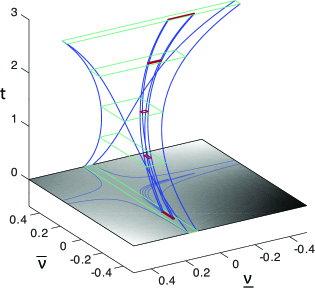
Figure 1: Four trajectories (heavy blue contours), plotted in coordinates $\left(\underline{\nu},\bar{\nu}\right)$, that bound a region specified by ${\underline{\nu}}_{T}=-1/6\pm 0.075$, ${\bar{\nu}}_{0}=-1/4\pm 0.05$. The steady state under the generating process sets ${\bm{\nu}}=1/6$. A time interval $T=3$ between the input distribution and the final-time generating function is shown. Small rectangles (heavy dark red) show the area $\delta\underline{\nu}\,\delta\bar{\nu}$ at five equally spaced times from start to end. The outer four trajectories (thin blue) show the possible range of joint images of $-\nicefrac{{1}}{{2}}\leq{\bar{\nu}}_{0}\leq\nicefrac{{1}}{{2}}$ and $-\nicefrac{{1}}{{2}}\leq{\underline{\nu}}_{T}\leq\nicefrac{{1}}{{2}}$. Large rectangles (thin green) show the constriction of the possible range $\propto e^{-T}$. Projections of the total range and the inner trajectories are shown in thin lines on the base plane. Shading of the base plane is a grayscale plot of ${\hat{\Phi}}_{0}^{2}$, which is constant along trajectories but variable over the $\left(\underline{\nu},\bar{\nu}\right)$ coordinate range. Min and max of ${\hat{\Phi}}_{0}^{2}$ are respectively $0.83$ and $1.1$.

VI.2.3 Invariant cumulant-generating function and the incompressible phase-space density

The stationary value of ${\hat{\Phi}}_{0}$, obtained from the gradient of ${\psi}_{0}$ with respect to the components ${\phi}^{\dagger}_{0a}$ and ${\phi}^{\dagger}_{0b}$, is computed in Eq. (186). It differs from unity – the reason constructions (102) and (103) were needed – and it is equal to the stationary value of $\hat{\Phi}$ at all times as a consequence of conservation of total number $N$. The value depends only on $\Lambda$ and $T$ in the combination

$${\hat{\Phi}}_{0}=\frac{1}{1+\Lambda e^{-T}}$$ (106)

Moreover, as a consequence of the conserved Liouville volume element from Eq. (105), the stationary-point evaluation of the CGF at all times takes the same form as Eq. (90) and evaluates to the constant

$$\frac{\psi}{N} =\log\left[\frac{{\underline{\nu}}_{a}}{{\bm{\nu}}_{a}}{\bar{\nu}}_{a}+\frac{{\underline{\nu}}_{b}}{{\bm{\nu}}_{b}}{\bar{\nu}}_{b}\right]$$

$$=-\log{\hat{\Phi}}_{0}$$ (107)

${\hat{\Phi}}_{0}$ in Eq. (106) is the basis for all information densities in this simple linear system. Through the stationary-point relation (59) between the Wigner function and the CGF, $-\log{\hat{\Phi}}_{0}$ is the incompressible phase-space density convected along stationary trajectories by Eq. (62). As shown below, it is also the geometrically invariant part of sole nonzero eigenvalue of the Fisher metric.

VI.3 Fisher metric

The Fisher metric (7) for the 2-state system evaluates, along the stationary path at any time, to

$$\frac{g}{N} =\frac{\partial\nu}{\partial\theta}\left[\begin{array}[]{r}1\\ -1\end{array}\right]\!\!\begin{array}[]{c}\left[\begin{array}[]{cc}1&-1\end{array}\right]\\ \phantom{[]}\end{array}$$ (113)

The nonzero eigenvalue comes from the single-argument generating function in Eq. (94) for the difference coordinate ${\rm n}$, and the zero eigenvalue comes from the linear CGF $hN$ for the conserved quantity $N$.

The term $\partial\nu/\partial\theta$ in Eq. (113) may be converted, after some algebra, to the form

$$\frac{\partial\nu}{\partial\theta} =\frac{\left(\frac{1}{4}-{\underline{\nu}}^{2}\right)\left(\frac{1}{4}-{\bar{\nu}}^{2}\right)}{\left(\frac{1}{4}-{\bm{\nu}}^{2}\right)}{\hat{\Phi}}_{0}^{2}$$ (114)

The measure terms $\left(\nicefrac{{1}}{{4}}-{\underline{\nu}}^{2}\right)$ and $\left(\nicefrac{{1}}{{4}}-{\bar{\nu}}^{2}\right)$ appearing in Eq. (114) follow the divisions (102) and (103) into independent dimensions of base and tilt variation, and we will show that their effects are canceled in an appropriate covariant derivative. The remaining dependence of the eigenvalue on the initial and final data is all carried in ${\hat{\Phi}}_{0}^{2}$.

VI.4 Dual coordinates for base and tilt, and the additive exponential family

To relate the Fisher metric in Eq. (113) to the construction of Sec. V.2 from the $\psi$-divergence and to dually-symplectic parallel transport, we first express the base and tilt displacements (102) and (103) in terms of the coordinates in their respective exponential families.

Introduce reference values for the fields $\theta$ and $h$ defined in Eq. (93), corresponding to the steady-state measure under the parameters of the generating process, denoted

$${\bm{\theta}} \equiv\log\left(\frac{\frac{1}{2}+{\bm{\nu}}}{\frac{1}{2}-{\bm{\nu}}}\right)$$

$${\bm{h}} \equiv\frac{1}{2}\log\left(\frac{1}{4}-{\bm{\nu}}^{2}\right)=-\log\left[2\operatorname{ch}\frac{{\bm{\theta}}}{2}\right]$$ (115)

It is clear, in the 2-argument generating function (90), that one component of variation in $z$ couples only to the conserved quantity $N$ and is not needed. It is sufficient therefore to vary along an affine coordinate in $z$ that couples to the dynamical argument ${\rm n}$, and the natural choice is to fix the component of $z$ corresponding to the component of ${\phi}^{\dagger}$ that is invariant under the stationary-path equations of motion, given in Eq. (182). The resulting contour for $z$ at final time $T$ becomes

$$z_{b}{\bm{\nu}}_{b}+z_{a}{\bm{\nu}}_{a} ={\Phi}^{\dagger}_{T}+{\bm{\nu}}{\phi}^{\dagger}_{T}=1$$

$$z_{b}-z_{a} ={\phi}^{\dagger}_{T}=\frac{{\underline{\nu}}_{T}-{\bm{\nu}}}{\frac{1}{4}-{\bm{\nu}}^{2}}$$ (116)

The quantity in the first line of Eq. (116) is preserved at all times by Eq. (182), and the quantity in the second line obeys the exponential law of Eq. (188) repeated as (105).

By the definition (102), the contour (116) which is affine in coherent-state fields ${\phi}^{\dagger}$ is written in the coordinates on the exponential family of tilts as

$$\underline{\nu} \equiv\frac{1}{2}\operatorname{th}\left(\frac{\theta+{\bm{\theta}}}{2}\right)$$

$$0 \equiv h+{\bm{h}}+\log\left[2\operatorname{ch}\left(\frac{\theta+{\bm{\theta}}}{2}\right)\right]$$

$$=h-\frac{1}{2}\log\left(\frac{1}{4}-{\underline{\nu}}^{2}\right)+\frac{1}{2}\log\left(\frac{1}{4}-{\bm{\nu}}^{2}\right)$$ (117)

Likewise, in the dual exponential representation (53) of the family of base distributions, the definition (103) giving the mean number offset in the nominal distribution is expressed

$$\bar{\nu} =\frac{1}{2}\operatorname{th}\left(\frac{\eta+{\bm{\theta}}}{2}\right)$$ (118)

in which $\eta\equiv\left({\eta}_{b}-{\eta}_{a}\right)$ in the dual action-angle system (53), analogously to $\theta$ in Eq. (93).

Because the two exponential coordinates (base and tilt) are additive, the mean of samples in the importance distribution can likewise be written

$$\nu =\frac{1}{2}\operatorname{th}\left(\frac{\theta+\eta+{\bm{\theta}}}{2}\right)$$ (119)

It follows that the eigenvalue (114) in the Fisher metric also has the simple expression

$$\frac{\partial\nu}{\partial\theta}=\frac{\partial\nu}{\partial\eta}=\frac{1}{4}-{\nu}^{2}$$ (120)

exhibiting the equivalence of the $\psi$-divergence expression (67) and the Hessian (69) for this quantity.

VI.5 Why coherent-state fields do not generally produce invertible coordinate transformations

The Hessian matrix is not a tensor under coordinate transform, so it is clear that the Hessian of $\psi$ with respect to the argument $z$ equivalent to the coherent-state response field ${\phi}^{\dagger}$ will not be the Fisher metric. However, since coherent states are in many ways a native basis for Doi-Peliti theory, as noted in Sec. V.5, we may ask whether some other coordinate duality can be defined from the coherent-state Hessian of $\psi$. In fact such a duality cannot generally be defined, and it is instructive to see where it fails, to better understand why the affine connection (88) and not the Fisher geometry captures the special role of coherent states.

A divergence under the Hessian of $\psi$ in coherent-state variables, which we will denote $\Delta\delta s^{2}$ for reasons to become clear in a moment, if converted from the coordinates $\underline{\nu}$ to coordinates $\theta$ along the $z$-affine contour (117), evaluates as

$$\frac{1}{N}\Delta ds^{2} \equiv{\left(\delta\theta\right)}^{2}{\left(\frac{1}{4}-{\underline{\nu}}^{2}\right)}^{2}\frac{{\partial}^{2}}{\partial{\underline{\nu}}^{2}}\left(\frac{\psi}{N}\right)$$

$$\equiv-{\left(\delta\theta\right)}^{2}{\left(\nu-\underline{\nu}\right)}^{2}$$ (121)

Unlike the Fisher metric, Eq. (121) is negative-semidefinite, and degenerates if $\nu=\underline{\nu}$, which is shown in Eq. (191) to hold for all $z$ if ${\bar{\nu}}_{0}={\bm{\nu}}$. At degenerate solutions, we cannot use the Hessian of $\psi$ to define a base-field variation $\delta\phi$ as a dual coordinate for a variation produced by a field $\delta{\phi}^{\dagger}$, as we could use the Hessian in the exponential family to produce a variation $\delta n$ as a dual coordinate to a variation $\delta\theta$.

The source of the degeneration has a nice description in terms of intrinsic and extrinsic curvatures, and advection, in the natural geometry on the exponential family. The geometric distance element (6), with $\theta$ and $h$ varied independently, is

$$\frac{1}{N}\delta s^{2} ={\left(\delta\theta\right)}^{2}\frac{{\partial}^{2}}{\partial{\theta}^{2}}\left(\frac{\psi}{N}-h\right)+{\left(\delta h\right)}^{2}\frac{{\partial}^{2}}{\partial h^{2}}h$$

$$={\left(\delta\theta\right)}^{2}\frac{\partial\nu}{\partial\theta}+{\left(\delta h\right)}^{2}0$$ (122)

The $z$-affine contour (117) specifies a function $h\!\left(\theta\right)$ with extrinsic curvature in the affine coordinate manifold of the exponential family, along which the distance element is

$$\frac{1}{N}\delta s^{2}_{\rm CS-ext} ={\left(\delta\underline{\nu}\right)}^{2}\frac{d^{2}}{d{\underline{\nu}}^{2}}\left(-h\!\left(\theta\right)\right)$$

$$={\left(\delta\theta\right)}^{2}\left(\frac{1}{4}+{\underline{\nu}}^{2}\right)$$ (123)

The second coherent-state coordinate derivative of $\psi$ along the contour (117) can be decomposed as

$$\frac{1}{N}\Delta\delta s^{2} ={\left(\delta\underline{\nu}\right)}^{2}\frac{d^{2}}{d{\underline{\nu}}^{2}}\left(\frac{\psi}{N}\right)$$

$$={\left(\delta\underline{\nu}\right)}^{2}\left[\frac{d^{2}}{d{\underline{\nu}}^{2}}\left(\frac{\psi}{N}-h\right)+\frac{d^{2}}{d{\underline{\nu}}^{2}}h\right]$$

$$={\left(\delta\theta\right)}^{2}\left(\frac{d^{2}}{d{\theta}^{2}}+2\underline{\nu}\frac{d}{d\theta}\right)\left(\frac{\psi}{N}-h\right)+{\left(\delta\underline{\nu}\right)}^{2}\frac{d^{2}}{d{\underline{\nu}}^{2}}h$$

$$={\left(\delta\theta\right)}^{2}\left[\frac{\partial\nu}{\partial\theta}+2\underline{\nu}\nu\right]+{\left(\delta\underline{\nu}\right)}^{2}\frac{d^{2}}{d{\underline{\nu}}^{2}}h$$

$$=\frac{1}{N}\left(\delta s^{2}-\delta s^{2}_{\rm CS-ext}\right)+{\left(\delta\theta\right)}^{2}2\underline{\nu}\nu$$ (124)

With some algebra, the expression (124) is shown to equal that in Eq. (121). The extrinsic curvature of the embedded contour $h\!\left(\theta\right)$ and the convected quantity $-2\underline{\nu}\nu$ cancel against the intrinsic Fisher curvature, rendering the duality invisible to the fields ${\phi}^{\dagger}$ at degenerate points.

VI.6 Flat transport in the coherent-state connection

The correct way to capture the simplifying role of coherent-state coordinates for simple models such as the 2-state system is with the dual connections of Sec. V.4.

We first recognize, from the forms (104) or (189) of $\Lambda$, a completely-descaled coordinate system for the dynamical parts of the coherent-state fields, define by

$$v \equiv\frac{\left(\underline{\nu}-{\bm{\nu}}\right)}{\sqrt{\frac{1}{4}-{\bm{\nu}}^{2}}} u \equiv\frac{\left(\bar{\nu}-{\bm{\nu}}\right)}{\sqrt{\frac{1}{4}-{\bm{\nu}}^{2}}}$$ (125)

The eigenvalue of the Fisher metric in Eq. (114) then reduces to

$$\frac{{\partial}^{2}}{\partial{\theta}^{2}}\!\left(\frac{{\psi}}{N}\right)=\frac{\left(dv/d\theta\right)\left(du/d\eta\right)}{{\left[1+uv\right]}^{2}}$$ (126)

The role of the factors $\left(\nicefrac{{1}}{{4}}-{\underline{\nu}}^{2}\right)=\sqrt{\nicefrac{{1}}{{4}}-{\bm{\nu}}^{2}}\left(\partial v/\partial\theta\right)$ and $\left(\nicefrac{{1}}{{4}}-{\bar{\nu}}^{2}\right)=\sqrt{\nicefrac{{1}}{{4}}-{\bm{\nu}}^{2}}\left(\partial u/\partial\eta\right)$ in Eq. (114) as measure terms is now explicit, and they can be absorbed by a change of variables to $u$ and $v$. By Eq. (189) and the definitions (125) and (106), $\left[1+uv\right]=\left[1+\Lambda e^{-T}\right]=1/{\hat{\Phi}}_{0}$, so the Fisher inner product (16) may be written

$$\delta\theta\,{\delta}_{\eta}n\left<\frac{\partial}{\partial\theta},\frac{\partial}{\partial n}\right>=\delta\underline{\nu}\,\delta\bar{\nu}\left<\frac{\partial}{\partial\underline{\nu}},\frac{\partial}{\partial\bar{\nu}}\right> =\delta u\,\delta v\,{\hat{\Phi}}_{0}^{2}$$ (127)

VI.6.1 Connection coefficients and absorption of measure terms

In this linear model, time evolution of ${\phi}^{\dagger}$ and $\phi$ has no cross-dependence once the initial values have been fixed through the gradients of ${\psi}_{0}$ as explained in Sec. VI.2.2. Thus ${\left({\nabla}^{\left(\eta\right)}_{k}\delta\theta\right)}^{j}=0$ and ${\left({\nabla}^{\left(\theta\right)\ast}_{k}\delta\eta\right)}^{j}=0$.

App. E.4 computes connection coefficients and covariant derivatives for the vector fields corresponding to Eq. (82), and for the metric tensor corresponding to Eq. (83). Eq. (199) in the appendix gives the covariant part of the time derivatives of $\delta\theta$ and $\delta\eta$ as

$$\left(\frac{\partial}{\partial\tau}\delta\theta\right)+\dot{\theta}\left({\nabla}_{\theta}\delta\theta\right) =\delta\theta$$

$$\left(\frac{\partial}{\partial t}\delta\eta\right)+\dot{\eta}\left({\nabla}^{\ast}_{\eta}\delta\eta\right) =-\delta\eta$$ (128)

capturing the simple exponential scaling (105) of the coherent-state fields in the exponential-family coordinates.

The covariant part of the change in the Fisher metric, from Eq. (83) is computed in Eq. (201) to be

$$\dot{\theta}{\nabla}_{\theta}g =\left(\dot{v}\frac{\partial}{\partial v}\log{\hat{\Phi}}_{0}^{2}\right)g$$

$$\dot{\eta}{\nabla}^{\ast}_{\eta}g =\left(\dot{u}\frac{\partial}{\partial u}\log{\hat{\Phi}}_{0}^{2}\right)g$$ (129)

Only the dependence in the Fisher eigenvalue ${\hat{\Phi}}_{0}^{2}$ from Eq. (127) appears.

The two lines of Eq. (129) (which are equal and opposite) scale as $\sim e^{-T}$, and have an interpretation similar to that of a Le Chatelier principle. The term $\Lambda e^{-T}$ in Eq. (106) for ${\hat{\Phi}}_{0}$ is a susceptibility of the initial stationary value ${\phi}_{0}$ to the perturbation by the tilt variable ${\phi}^{\dagger}_{T}=z$, attenuated exponentially from time $T$ to time $0$. The role of this attenuation, which takes ${\hat{\Phi}}_{0}\rightarrow 1$ as $T\rightarrow\infty$, becomes clearer as a constraint on the total extractable information when we consider in Sec. VI.7 the range of all initial distributions ${\rho}_{0}$ and all tilts $z$.

VI.6.2 Duality of dynamics and inference in Doi-Peliti theory

The natural separation of the coordinate transformation of the inner product of vector fields $\delta\theta$ and $\delta\eta$ generated by time translation is not between exponential and mixture coordinates, as in the dually-flat connections of Amari Amari:inf_geom:01 , but rather between the symplectically dual contributions from changes in $\theta$ and in $\eta$. The two contributions group as

$$0 =\frac{d}{dt}\left(\delta\theta\,g\,\delta\eta\right)$$

$$=\left(\frac{\partial}{\partial t}\delta\theta\right){\delta}_{\eta}\nu+\dot{\theta}{\nabla}^{\left(\theta\right)}_{\theta}\!\left(\delta\theta\,g\right)\delta\eta$$

$$\mbox{}+{\delta}_{\theta}\nu\left(\frac{\partial}{\partial t}\delta\eta\right)+\delta\theta\,\dot{\eta}{\nabla}^{\left(\eta\right)\ast}_{\eta}\!\left(g\,\delta\eta\right)$$ (130)

The two rows of Eq. (130) add covariant contributions from Eq. (128) and Eq. (129) in the combinations

$$\left(\frac{\partial}{\partial t}\delta\theta\right){\delta}_{\eta}\nu+\dot{\theta}{\nabla}^{\left(\theta\right)}_{\theta}\!\left(\delta\theta\,g\right)\delta\eta =\left(\delta\theta\,{\delta}_{\eta}\nu\right)\left(1+\dot{v}\frac{\partial}{\partial v}\log{\hat{\Phi}}_{0}^{2}\right)$$

$${\delta}_{\theta}\nu\left(\frac{\partial}{\partial t}\delta\eta\right)+\delta\theta\,\dot{\eta}{\nabla}^{\left(\eta\right)\ast}_{\eta}\!\left(g\,\delta\eta\right) =\left({\delta}_{\theta}\nu\,\delta\eta\right)\left(-1+\dot{u}\frac{\partial}{\partial u}\log{\hat{\Phi}}_{0}^{2}\right)$$ (131)

Eq. (131) captures in the clearest way possible the symplectic balance of distribution dynamics (through $\eta$) and inference (through $\theta$) in Doi-Peliti theory, through both the direct effects of the exponential growth and decay eigenvalues $\left(\pm 1\right)$ and the Le Chatelier-like susceptibility of the density ${\hat{\Phi}}_{0}$.

VI.7 The Fisher information density and large-deviation ratios as sample estimators

The interpretation of the vector inner product as a convected density of information can be illustrated by using ratios of large-deviation probabilities to define a sample estimator for differences in the tilt coordinate $\eta$ between two base distributions.

Suppose that we sample from a binomial nominal distribution at a parameter $\eta$ that is to be estimated. Recall from Eq. (28) that the probability for the value ${\rm n}$ of a sample to exceed a threshold $n$ is given in terms of the large-deviation function by

$$P\!\left({\rm n}\geq n\mid\eta\right)\sim e^{-{\psi}^{\ast}\left(n;\eta\right)}$$ (132)

In a 1-dimensional system, for two threshold values $n_{B}>n_{A}$, the conditional probability for ${\rm n}$ to surpass $n_{B}$ given that it has surpassed $n_{A}$ is the ratio

$$P\!\left(n_{B}\mid n_{A};\eta\right) \equiv\frac{P\!\left({\rm n}\geq n_{B}\mid\eta\right)}{P\!\left({\rm n}\geq n_{A}\mid\eta\right)}$$

$$\sim e^{-\left[{\psi}^{\ast}\left(n_{B};\eta\right)-{\psi}^{\ast}\left(n_{A};\eta\right)\right]}$$ (133)

The ratio (133) can be estimated from samples of the indicator function $h_{{\rm n}}$ for thresholds $n$ as described in Sec. III.2.

App. E.5 shows that if two such conditional probabilities are compared from distributions at unknown parameters ${\eta}_{2}$ and ${\eta}_{1}$, the log ratio is related to the large-deviation thresholds and the $\eta$ values as

$$\log\left(\frac{P\!\left(n_{B}\mid n_{A};{\eta}_{2}\right)}{P\!\left(n_{B}\mid n_{A};{\eta}_{1}\right)}\right) \sim\int_{{\eta}_{1}}^{{\eta}_{2}}\!\!\int_{n_{A}}^{n_{B}}d_{\theta}n\,d\eta$$

$$=\left(n_{B}-n_{A}\right)\left({\eta}_{2}-{\eta}_{1}\right)$$ (134)

where $d_{\theta}n\,d\eta$ is one of the two forms of the (differential) inner product appearing in Eq (74).

Thus

$$\frac{\log\left(\frac{P\!\left(n_{B}\mid n_{A};{\eta}_{2}\right)}{P\!\left(n_{B}\mid n_{A};{\eta}_{1}\right)}\right)}{\left(n_{B}-n_{A}\right)}\sim\left({\eta}_{2}-{\eta}_{1}\right)$$ (135)

is a sample estimator for the difference of exponential parameters in the two underlying distributions.

The quantity (134) may be computed at any time, for instance the final time $T$ when the thresholds $n_{B}$ and $n_{A}$ are imposed as experimental conditions, and ${\eta}_{2}$ and ${\eta}_{1}$ characterize evolved nominal distributions at time $T$ from any pair of initial conditions at some earlier time $t=0$. If we use the stationary-path conditions to propagate values of $\theta$ and $\eta$ through time, and define $V\!\left(\tau\right)$ to be the area inside the image of the rectangle in Eq. (134) along these stationary trajectories, time-invariance of the inner product, and the Liouville conservation of volume elements in dual coordinates, implies that

$$\frac{d}{d\tau}\int_{V}d_{\theta}n\,d\eta=0$$ (136)

Note that, with a coordinate transform to coherent-state variables and a corresponding redefinition of the boundary of $V$, the relation (136) could be recast using Eq. (127) as

$$\frac{d}{d\tau}\int_{V}dv\,du\,{\hat{\Phi}}_{0}^{2}=0$$ (137)

which is the conserved integral graphed in Fig 1.

In Eq. (137) ${\hat{\Phi}}_{0}^{2}$, the 2-dimensional differential of the scaled CGF $\psi/N=-\log{\hat{\Phi}}_{0}$, appears explicitly as the density of overlap of $dv$ with $du$ that, like $\psi$ itself, is constant along stationary paths. ${\hat{\Phi}}_{0}^{2}$ is not independent of the position $\left(v,u\right)$ within the volume $V$, but because the volume element moves along with the conserved density, the integral measures a fixed quantity of Fisher information as it is transported through different domains of base and tilt.

Although the limits of integration for $\int dv\,du$ in Eq. (137) are bounded, the limits on $\left({\eta}_{2}-{\eta}_{1}\right)$ in Eq. (134) are not, so formally the range of the sample estimator (135) remains unbounded over any duration $T$. However, for any fixed values of ${\left(n_{B}-n_{A}\right)}_{t=T}$ and starting uncertainty ${\left({\eta}_{2}-{\eta}_{1}\right)}_{t=0}$, the total information obtainable from large-deviations sampling about differences in the initial conditions is finite and decreases as $e^{-T}$. In Fig 1 this limit is seen in the way any fixed ranges are squeezed exponentially at the “waist” as $T\rightarrow\infty$. The contraction of boundaries, rather than the asymptotic behavior of the eigenvalue in the Fisher metric, measures the loss of information between initial distributions and final observations with increasing separation between the two.

VII Conclusions: the duality of dynamics and inference for irreversible and reversible processes

The three-part structure of the Fisher metric, dual Riemannian connections, and symplectic parallel transport of the Wigner density, vector fields, and the metric tensor, elegantly expresses the transport properties along 2FFI stationary paths in terms of geometric invariants. It resolves a feature of 2-field constructions that at first seems paradoxical: if memory of initial conditions is continuously lost to dissipation, what concept of time-reversal is implied by invertibility of the map along stationary rays? The answer from the perspective of importance sampling is that, even if samples are finite, their expectations are computed in continuous-valued distributions, and deformations of measure through the Radon-Nikodym derivative can locally compensate for concentration of measure in the nominal distribution by expanding sensitivity of likelihood ratios. Locally in sampling space, then, time is immaterial as it is in Hamiltonian mechanics; the mappings along stationary trajectories make it possible to interpret sampling protocols from different times in an evolving distribution simply as coordinate transformations of a fixed sampling protocol on the original distribution. On the other hand, for any fixed ranges of parameter variation in the initial conditions, and fixed large-deviation thresholds compared at late time, the integrated Liouville density contracts monotonically with the separation between the two times, reflecting the absolute loss of information that can be recovered.

We have wanted to establish a concrete interpretation of time-duality in 2FFI theories as a duality of dynamics and inference, to provide an alternative to the interpretation in terms of physical reversal of paths that is the starting point in most of the literature on fluctuation theorems in stochastic thermodynamics. Microscopic reversibility can always be added later to any class of 2FFI constructions as a restriction on the scope of phenomena under study, and both stronger conclusions and additional interpretations will then follow from the added constraints. Where the existence of a duality in the mathematics itself does not depend on any such additional assumptions, taking the inference interpretation to reflect the core concepts, directly expressing Kolmogorov’s forward/backward adjoint duality, frames the special case of microscopic reversibility as one in which the system’s own dynamics contains an image of certain sampling protocols over itself.

Even if one only cares about microscopically reversible processes, making explicit the step of self-modeling, and having a concrete interpretation of conserved densities such as the Fisher information constructed here, provides a bridge between trajectory reversal in low-level mechanics and operations for sample estimation of the kind that are used by control systems. Linking limitations from path probability in a system’s autonomous dynamics to concepts of information capacity in control loops Ashby:cybernetics:56 ; Ashby:req_var:58 ; Conant:regulator:70 promises a way to study the limits on spontaneous emergence of dynamical hierarchy, which has been a desired application for stochastic thermodynamics England:statphys_selfrepl:13 ; Perunov:adaptation:15 . These are intended topics for future work.

Acknowledgments

The author thanks Supriya Krishnamurthy for ongoing collaboration and the Stockholm University Physics Department for hospitality while much of this work was done, and Nathaniel Virgo for helpful discussion. The work was supported in part by NASA Astrobiology CAN-7 award NNA17BB05A through the College of Science, Georgia Institute of Technology, and by the Japanese Ministry of Education, Culture, Sports, Science, and Technology (MEXT) through the World Premiere International program.

Appendix A Fisher spherical embeddings

A.1 The embedding for general distributions on finite state spaces

Eq. (6) in the text can be written in the form

$$\delta s^{2}=4\delta{\theta}^{i}\delta{\theta}^{j}\sum_{{\rm n}}\frac{\partial\sqrt{{\tilde{\rho}}_{{\rm n}}^{\left(\theta\right)}}}{\partial{\theta}^{i}}\frac{\partial\sqrt{{\tilde{\rho}}_{{\rm n}}^{\left(\theta\right)}}}{\partial{\theta}^{j}}$$ (138)

Let $\left|\left\{{\rm n}\right\}\right|$ be the cardinality of the set of states on which ${\rho}_{{\rm n}}$ is defined (for example, in chemistry, only a sub-lattice of all integer-valued vectors in the positive orthant may ever be accessible as counts, given a system’s stoichiometry and conserved quantities). Suppose $\left|\left\{{\rm n}\right\}\right|$ is finite in order illustrate the Fisher embedding geometry for distributions over finite state spaces. All possible base distributions $\rho$ fall within the simplex of dimension $\left|\left\{{\rm n}\right\}\right|-1$.

Now let $\left\{{\alpha}_{1},{\alpha}_{2},\ldots{\alpha}_{\left|\left\{{\rm n}\right\}\right|-1}\right\}$ be angles associated with independent rotation axes in ${\mathbb{R}}^{\left|\left\{{\rm n}\right\}\right|}$. Any distribution can be embedded in ${\mathbb{R}}^{\left|\left\{{\rm n}\right\}\right|}$ by arranging the states ${\rm n}$ in an (arbitrary) order ${{\rm n}}_{1},{{\rm n}}_{2},\ldots{{\rm n}}_{\left|\left\{{\rm n}\right\}\right|}$, and writing

$$p_{{{\rm n}}_{1}} \equiv\cos^{2}{\alpha}_{1}$$

$$p_{{{\rm n}}_{2}} \equiv\sin^{2}{\alpha}_{1}\cos^{2}{\alpha}_{2}$$

$$p_{{{\rm n}}_{3}} \equiv\sin^{2}{\alpha}_{1}\sin^{2}{\alpha}_{2}\cos^{2}{\alpha}_{3}$$

$$\>\>\vdots$$

$$p_{{{\rm n}}_{\left|\left\{{\rm n}\right\}\right|-1}} \equiv\sin^{2}{\alpha}_{1}\sin^{2}{\alpha}_{2}\cdots\sin^{2}{\alpha}_{\left|\left\{{\rm n}\right\}\right|-2}\cos^{2}{\alpha}_{\left|\left\{{\rm n}\right\}\right|-1}$$

$$p_{{{\rm n}}_{\left|\left\{{\rm n}\right\}\right|}} \equiv\sin^{2}{\alpha}_{1}\sin^{2}{\alpha}_{2}\cdots\sin^{2}{\alpha}_{\left|\left\{{\rm n}\right\}\right|-2}\sin^{2}{\alpha}_{\left|\left\{{\rm n}\right\}\right|-1}$$ (139)

A recursive calculation gives the line element (138) in terms of the angle coordinates on the radius-2 sphere as

$$\delta s^{2} =4\left[\vphantom{\delta{\alpha}_{\left|\left\{{\rm n}\right\}\right|}^{2}}\delta{\alpha}_{1}^{2}+\sin^{2}{\alpha}_{1}\,\delta{\alpha}_{2}^{2}+\ldots\right.$$

$$\mbox{}+\left.\left(\sin^{2}{\alpha}_{1}\ldots\sin^{2}{\alpha}_{\left|\left\{{\rm n}\right\}\right|-2}\right)\delta{\alpha}_{\left|\left\{{\rm n}\right\}\right|-1}^{2}\right]$$ (140)

A.2 Embeddings in reduced dimension for exponential families on the multinomial

The Poisson (13) and multinomial (14) distributions are both in a class recognized by Anderson, Craciun, and Kurtz (ACK) Anderson:product_dist:10 in connection with uniqueness of stationary solutions for chemical reaction networks. All factorial moments are powers their first moments, causing the CGF for many particles to scale as a multiple of a single-particle CGF. It is not then surprising that the expression (6) for the Fisher metric in terms of a distribution ${\tilde{\rho}}_{{\rm n}}$ with possibly indefinitely many independent terms, for the ACK distributions projects to a function of the same form in terms of expected numbers $n_{i}$ over the $D$ independent species.

To see how this works for a distribution ${\rho}^{\left(n_{0}\right)}_{{\rm n}}$ with multinomial form (14), express the expected number fractions as

$$\frac{n_{0i}}{N}=\frac{e^{{\eta}_{i}}}{\sum_{j=1}^{D}e^{{\eta}_{j}}}$$ (141)

Then the mean in the distribution ${\tilde{\rho}}_{{\rm n}}^{\left(\theta;n_{0}\right)}$ is

$$\frac{n_{i}\!\left(\theta\right)}{N}=\frac{e^{{\eta}_{i}+{\theta}_{i}}}{\sum_{j=1}^{D}e^{{\eta}_{j}+{\theta}_{j}}}\equiv{\nu}_{i}$$ (142)

and the CGF $\psi\!\left(\theta;n_{0}\right)$ evaluates (up to a constant offset) to

$$\psi\!\left(\theta;n_{0}\right)=N\log\left[\sum_{j=1}^{D}e^{{\eta}_{j}+{\theta}_{j}}\right]$$ (143)

The Hessian giving the Fisher metric is

$$g_{ij}\!\left(\theta\right)=N\left\{{\nu}_{i}{\delta}_{ij}-{\nu}_{i}{\nu}_{j}\right\}$$ (144)

where ${\nu}_{i}$ is the function of $\eta+\theta$ in Eq. (142). Inverting Eq. (144), and projecting onto the $\sum_{i}{\theta}_{i}=0$ to fix the undetermined component of $\theta$, gives the inverse

$$g^{ij}\!\left(n\right)=\frac{1}{N}\left\{\frac{1}{{\nu}_{i}}{\delta}_{ij}-\frac{1}{D}\left[\frac{1}{{\nu}_{i}}+\frac{1}{{\nu}_{j}}-\frac{1}{D}\sum_{k}\frac{1}{{\nu}_{k}}\right]\right\}$$ (145)

One can check that both $g\!\left(\theta\right)$ and $g^{-1}\!\left(n\right)$ sum to zero on either index, and the product

$$g^{ij}\!\left(n\right)g_{jk}\!\left(\theta\right)={\delta}^{i}_{k}-\frac{1}{D}$$ (146)

is the identity on the subspace $\sum_{j=1}^{D}{\theta}^{j}=0$ or $\sum_{j=1}^{D}n_{j}=N$.

If a shift of the tilted distribution in the exponential family is indexed with coordinate $\delta n$, with $\sum_{j=1}^{D}\delta n_{j}=0$, the Fisher distance element from Eq. (12) becomes

$$\delta s^{2}=\sum_{j=1}^{D}\frac{\delta n_{j}^{2}}{n_{j}}$$ (147)

which is the same function of $n$ as the function of $\tilde{\rho}$ in the third line of Eq. (6).

Appendix B Sample means and variances in the large-deviation approximation to threshold indicator expectations

The expectation of the tilted indicator function from Eq. (27) may be written in a series of inequalities culminating in the expression for the CGF, as

$${\left<{\tilde{h}}^{\theta}\right>}_{\left(\theta;n_{0}\right)} =\sum_{{\rm n}>\bar{n}}e^{-\theta{\rm n}}e^{\theta{\rm n}}{\rho}^{\left(n_{0}\right)}_{{\rm n}}$$

$$\leq e^{-\theta\bar{n}}\sum_{{\rm n}>\bar{n}}e^{\theta{\rm n}}{\rho}^{\left(n_{0}\right)}_{{\rm n}}$$

$$\leq e^{-\theta\bar{n}}\sum_{{\rm n}}e^{\theta{\rm n}}{\rho}^{\left(n_{0}\right)}_{{\rm n}}$$

$$=e^{\psi\left(\theta;n_{0}\right)-\theta\bar{n}}$$ (148)

providing Eq. (28) in the text.

The variance of the same sample estimator has a corresponding bound

$${\left<{\left({\tilde{h}}^{\theta}\right)}^{2}\right>}_{\left(\theta;n_{0}\right)}-{\left<{\tilde{h}}^{\theta}\right>}_{\left(\theta;n_{0}\right)}^{2} ={\left<{\left({\tilde{h}}^{\theta}\right)}^{2}\right>}_{\left(\theta;n_{0}\right)}-{\left<h\right>}_{\left(n_{0}\right)}^{2}$$

$$={\left<e^{\psi\left(\theta;n_{0}\right)-\theta{\rm n}}{\tilde{h}}^{\theta}\right>}_{\left(\theta;n_{0}\right)}-{\left<h\right>}_{\left(n_{0}\right)}^{2}$$

$$\leq e^{\psi\left(\theta;n_{0}\right)-\theta\bar{n}}{\left<{\tilde{h}}^{\theta}\right>}_{\left(\theta;n_{0}\right)}-{\left<h\right>}_{\left(n_{0}\right)}^{2}$$

$$=e^{\psi\left(\theta;n_{0}\right)-\theta\bar{n}}{\left<h\right>}_{\left(n_{0}\right)}-{\left<h\right>}_{\left(n_{0}\right)}^{2}$$ (149)

giving Eq. (29) in the text.

To estimate the tightness of the bounds, begin by observing that in the large-deviation scaling regime (31), with all cumulants generated as derivatives of $\psi\sim N$, the expansion of central moments in terms of cumulants bounds the scaling of the $k$th central moment as

$$\left<{\left({\rm n}-\left<{\rm n}\right>\right)}^{k}\right>/{\left<{\rm n}\right>}^{k}\leq\mathcal{O}\!\left(N^{-\left\lceil k/2\right\rceil}\right)$$ (150)

The log ratio we wish to bound is the Bregman divergence

$$\log\left[\frac{\sum_{{\rm n}>\bar{n}}e^{-\theta\left({\rm n}-\bar{n}\right)}e^{\theta{\rm n}}{\rho}_{{\rm n}}}{\sum_{{\rm n}}e^{\theta{\rm n}}{\rho}_{{\rm n}}}\right]=\theta\bar{n}-\psi\!\left(\theta,n_{0}\right)+\log{\left<h^{\left(\bar{n}\right)}\right>}_{\left(n_{0}\right)}$$ (151)

The maximum of Eq. (151) occurs at $\theta\!\left(\bar{n}\right)$ from Eq. (9), and the width of the transition for the log ratio to change by $\mathcal{O}\!\left(N^{0}\right)$ is given by

$$\delta\theta\approx{\left({\left.\frac{{\partial}^{2}\psi}{{\partial\theta}^{2}}\right|}_{\theta\left(\bar{n}\right)}\right)}^{-1}\sim N^{-1/2}$$ (152)

To estimate its maximum value we write Eq. (151) as the sum of log ratios of the two inequalities in Eq. (148), and observe that they have boundary values

$${\left.\log\left[\frac{\sum_{{\rm n}>\bar{n}}e^{-\theta\left({\rm n}-\bar{n}\right)}e^{\theta{\rm n}}{\rho}_{{\rm n}}}{\sum_{{\rm n}>\bar{n}}e^{\theta{\rm n}}{\rho}_{{\rm n}}}\right]\right|}_{\theta=0} =0$$

$${\left.\log\left[\frac{\sum_{{\rm n}>\bar{n}}e^{\theta{\rm n}}{\rho}_{{\rm n}}}{\sum_{{\rm n}}e^{\theta{\rm n}}{\rho}_{{\rm n}}}\right]\right|}_{\theta\rightarrow\infty} =0$$ (153)

The values of these ratios at intermediate $\theta$ are then obtained by integrating the derivatives

$$\frac{\partial}{\partial\theta}\log\left[\frac{\sum_{{\rm n}>\bar{n}}e^{-\theta\left({\rm n}-\bar{n}\right)}e^{\theta{\rm n}}{\rho}_{{\rm n}}}{\sum_{{\rm n}>\bar{n}}e^{\theta{\rm n}}{\rho}_{{\rm n}}}\right] =-\frac{\sum_{{\rm n}>\bar{n}}\left({\rm n}-\bar{n}\right)e^{\theta{\rm n}}{\rho}_{{\rm n}}}{\sum_{{\rm n}>\bar{n}}e^{\theta{\rm n}}{\rho}_{{\rm n}}}$$

$$\frac{\partial}{\partial\theta}\log\left[\frac{\sum_{{\rm n}>\bar{n}}e^{\theta{\rm n}}{\rho}_{{\rm n}}}{\sum_{{\rm n}}e^{\theta{\rm n}}{\rho}_{{\rm n}}}\right] =\frac{\sum_{{\rm n}>\bar{n}}\left({\rm n}-n\!\left(\theta\right)\right)e^{\theta{\rm n}}{\rho}_{{\rm n}}}{\sum_{{\rm n}>\bar{n}}e^{\theta{\rm n}}{\rho}_{{\rm n}}}$$ (154)

Both log derivatives in Eq. (154) are monotone if $\psi$ is convex, and their values sum to $\bar{n}-n\!\left(\theta\right)$, the derivative of Eq (151), where $n\!\left(\theta\right)\equiv{\left<{\rm n}\right>}_{{\tilde{\rho}}^{\left(\theta,n_{0}\right)}}$.

Next, observe the leading-order scaling of the expectation ${\left<{\left({\rm n}-\bar{n}\right)}^{2}\right>}_{{\rm n}>\bar{n}}\approx{\left<\left({\rm n}-\bar{n}\right)\right>}^{2}_{{\rm n}>\bar{n}}$ on the half-line (as for any second moment), and likewise for $\left({\rm n}-n\!\left(\theta\right)\right)$.

At $\theta\!\left(\bar{n}\right)$, where $n\!\left(\theta\right)=\bar{n}$, the two derivatives (154) are equal and opposite, and the boundary of the half-line ${\rm n}>\bar{n}$ is also the symmetry point of ${\left({\rm n}-\bar{n}\right)}^{2}$. Because the skewness and higher-order central moments grow more slowly than ${\bar{n}}^{k}$ by Eq. (150), ${\left<{\left({\rm n}-\bar{n}\right)}^{2}\right>}_{{\rm n}>\bar{n}}\approx{\left<{\left({\rm n}-\bar{n}\right)}^{2}\right>}_{{\rm n}}\times\left\{1+\mathcal{O}\!\left(1/N\right)\right\}$, and given the large-deviations scaling of central moments (150), the derivatives in Eq. (154) scale as

$${\left.\frac{\sum_{{\rm n}>\bar{n}}\left({\rm n}-\bar{n}\right)e^{\theta{\rm n}}{\rho}_{{\rm n}}}{\sum_{{\rm n}>\bar{n}}e^{\theta{\rm n}}{\rho}_{{\rm n}}}\right|}_{n\left(\theta\right)=\bar{n}}\sim\sqrt{\left<{\left({\rm n}-\bar{n}\right)}^{2}\right>}\sim N^{1/2}$$ (155)

Over the range $\pm\delta\theta$ from Eq. (152), where the total log ratio changes by $\mathcal{O}\!\left(N^{0}\right)$, the integral of the first derivative (155) saturates the lower limit in the first line of Eq. (153), and the upper limit in the second line of Eq. (153), to within $\leq\mathcal{O}\!\left(N^{1/2}\right)$, implying that the log-ratios themselves at the midpoint scale as $\leq\mathcal{O}\!\left(N^{1/2}\right)$. Hence also the total log ratio that is their sum scales as $\log\left[{\left<h^{\left(\bar{n}\right)}\right>}_{\left(n_{0}\right)}/e^{-{\psi}^{\ast}\left(\bar{n}\right)}\right]\leq\mathcal{O}\!\left(N^{1/2}\right)$, the result used in the text.

Appendix C Review of Doi Hilbert space and Peliti functional integral constructions

C.1 Doi operator algebra and inner product

The main constructs in the Doi operator formulation Doi:SecQuant:76 ; Doi:RDQFT:76 of moment-generating functions as formal power series are as follows:

The identification (34) of $z$ and $\partial/\partial z$ with raising and lowering operators $a^{\dagger}$ and $a$ allows the commutator algebra

$$\left[a_{i},a^{\dagger}_{j}\right]={\delta}_{ij}.$$ (156)

to stand for the commutator algebra between components of $\partial/\partial z$ and factors of $z$, applied by function composition acting to the right on MGFs.

Monomials $z^{{\rm n}}$ from Eq. (1) are basis elements in a linear space of MGFs, built up by multiplication on the number 1. A bracket notation for states and an inner product are introduced by the pair of denotations

$$1 \rightarrow\left|0\right) \int d^{D}\!z\,{\delta}^{D}\!\left(z\right) \rightarrow\left(0\right|$$ (157)

Each monomial $z^{{\rm n}}$ is denoted as a number state

$$\prod_{i=1}^{D}z_{i}^{{{\rm n}}_{i}}\times 1 \rightarrow\prod_{i=1}^{D}{a_{i}^{\dagger}}^{{{\rm n}}_{i}}\left|0\right)\equiv\left|{\rm n}\right).$$ (158)

The number states are eigenstates of the set of number operators ${\hat{n}}_{i}\equiv a^{\dagger}_{i}a^{i}$ (no Einstein sum):

$${\hat{n}}_{i}\left|{\rm n}\right)={{\rm n}}_{i}\left|{\rm n}\right).$$ (159)

Dual to each number state is a conjugate projection operator

$$\left({\rm m}\right| \equiv\left(0\right|\prod_{i=1}^{D}\frac{{a_{i}^{\dagger}}^{{\rm m}_{i}}}{{\rm m}_{i}!}\leftarrow\int d^{D}\!z\,{\delta}^{D}\!\left(z\right)\prod_{i=1}^{D}\frac{{\left(\partial/\partial z_{i}\right)}^{{\rm m}_{i}}}{{\rm m}_{i}!}$$ (160)

From the commutation relations of variables and their derivatives it follows that the number states and projectors have overlap

$$\left({\rm m}\,\right|\!\left.{\rm n}\right)={\delta}^{D}_{{\rm m}{\rm n}}$$ (161)

the Kronecker $\delta$ symbol on $D$ indices. The number states and projectors are complete, and a sum of Eq. (161) on ${\rm m}$ is the Glauber norm

$$\left(0\right|e^{\sum_{i}a_{i}}\left|{\rm n}\right)=1,\quad\forall{\rm n},$$ (162)

which defines the asymmetric inner product on the Hilbert space of generating functions.

Replacing the uniform measure $\sum_{i}a_{i}\equiv 1^{T}a$ in Eq. (162) with the scalar product $za$ gives the map (37) to $\Psi\!\left(z\right)$ in the main text. $\Psi\!\left(1\right)\equiv 1$; the Glauber norm of the Laplace transform of any normalized distribution is the trace of the probability distribution $\sum_{{\rm n}}{\rho}_{{\rm n}}$.

C.2 Coherent states and Peliti functional integral

The uniform measure in the 2D-dimensional integral for the representation of unity (43) in the main text is known as the Haar measure. Using the definition (40) for coherent states and (41) for their dual projectors, and expanding the exponential functions as sums,

$$\int\frac{d^{D}\!{\phi}^{\dagger}d^{D}\!\phi}{{\pi}^{D}}\left|\phi\right)\left(\phi\right|$$

$$=\int\frac{d^{D}\!{\phi}^{\dagger}d^{D}\!\phi}{{\pi}^{D}}\prod_{i=1}^{D}e^{-{\phi}^{\dagger}_{i}{\phi}_{i}}\sum_{{{\rm n}}_{i}}\sum_{{\rm m}_{i}}\frac{{\phi}_{i}^{{{\rm n}}_{i}}{{\phi}^{\dagger}_{i}}^{{\rm m}_{i}}}{{{\rm n}}_{i}!}\left|{\rm n}\right)\left({\rm m}\right|$$

$$=\sum_{{\rm n}}\left|{\rm n}\right)\left({\rm n}\right|=I$$ (163)

The phase component in each integral $d{\phi}^{\dagger}_{i}\,d{\phi}_{i}$ vanishes unless ${{\rm n}}_{i}={\rm m}_{i}$, and the remaining modulus component produces a Gamma-function canceling the ${{\rm n}}_{i}!$. Thus the Haar measure on coherent states is equivalent to the uniform measure on states ${\rm n}$ of the classical probability distribution.

Mapping backward through the correspondences between analytic functions and Doi state vectors from App. C.1, an evaluation of the integral in terms of Dirac $\delta$-functions shows that the effect of the representation of unity is the map

$$\int\frac{d^{D}{\phi}^{\dagger}d^{D}\phi}{{\pi}^{D}}\left|\phi\right)\left({\phi}^{\dagger}\right|$$

$$\leftarrow\int\frac{d^{D}{\phi}^{\dagger}d^{D}\phi}{{\pi}^{D}}e^{z^{\prime}\phi}1\int d^{D}\!z\,{\delta}^{D}\!\left(z\right)e^{{\phi}^{\dagger}\left(\partial/\partial z-\phi\right)}$$

$$=\int d^{D}\!z\,{\delta}^{D}\!\left(z\right)e^{z^{\prime}\partial/\partial z}$$

$$=z\mapsto z^{\prime}$$ (164)

To keep track of the scoping rules for application of complex functions and derivatives would require introducing a distinct set of variables $z_{k\delta t}$ for each interval in the quadrature (38). In the Doi operator algebra this scoping is handled by the bracket inner product, and the map (164) becomes simply the identity map on $a^{\dagger}$ and $a$.

The integration measure that results from inserting a copy of the representation of unity (43) between each interval of time evolution in Eq. (38) is called a skeletonized measure. Its limit as the interval length $\delta t\rightarrow 0$

$$\int_{0}^{T}{\mathcal{D}}^{D}\!{\phi}^{\dagger}{\mathcal{D}}^{D}\!{\phi}\equiv\lim_{\delta t\rightarrow 0}\prod_{k=1}^{T/\delta t}\int\frac{d^{D}\!{\phi}^{\dagger}_{k\delta t}d^{D}\!{\phi}_{k\delta t}}{{\pi}^{D}}$$ (165)

defines the functional integration measure used in Eq. (44) and elsewhere.

Appendix D Stationary-point approximations to the Wigner function

The functional integral provides the most direct route to the current conservation law (60) for the Wigner function. It is possible, with somewhat more work, to derive the same relations directly from stationary variation of the generating function, and in the process to gain some more intuition for what the Wigner function quantifies.

The Wigner function in terms of an explicit density over coherent-state parameters

Begin by writing any state vector as the integral of a density in the coherent-state basis:

$$\left|\Psi\right)\equiv\int d^{D}\!\phi\,\left|\phi\right)\rho\!\left(\phi\right)$$ (166)

The generalized Glauber norm (37) returns the analytic representation of the MFG:

$$\Psi\!\left(z\right) =\left(0\right|e^{za}\left|\Psi\right)$$

$$=\int d^{D}\!\phi\,\left(0\right|e^{za}\left|\phi\right)\rho\!\left(\phi\right)$$

$$=\int d^{D}\!\phi\,e^{\left(z-1\right)\phi}\rho\!\left(\phi\right)$$ (167)

Now evaluate the integral in Eq. (57) at time $t\rightarrow T$, where the stationary value of the field ${\phi}^{\dagger}$ will coincide with the imposed argument $z$,

$$w_{T}\!\left({\phi}^{\dagger}_{\ddagger},{\phi}_{\ddagger}\right) =\frac{1}{{\pi}^{D}}\int d^{D}\!\phi\,e^{\left({\phi}^{\dagger}_{\ddagger}-z\right)\left(\phi-{\phi}_{\ddagger}\right)}e^{\left(z-1\right)\phi}\rho\!\left(\phi\right)$$ (168)

It follows then that

$$\int d^{D}\!{\phi}^{\dagger}_{\ddagger}\,w_{T}\!\left({\phi}^{\dagger}_{\ddagger},{\phi}_{\ddagger}\right)=e^{\left(z-1\right){\phi}_{\ddagger}}\rho\!\left({\phi}_{\ddagger}\right)$$ (169)

A second integral over the ${\phi}_{\ddagger}$ fields yields the two equivalent expressions (58) and (167).

Stationary-point approximations

The stationary value $\bar{\phi}\!\left(z\right)$ of the tilted density $e^{\left(z-1\right)\phi}\rho\!\left(\phi\right)$ is given by

$${\left.\frac{\partial\log\rho}{\partial\phi}\right|}_{\bar{\phi}\left(z\right)}=1-z$$ (170)

The two stationarity conditions on the arguments of $w_{T}$ follow from Eq. (168) as

$${\left.\frac{\partial}{\partial{\phi}_{\ddagger}}w_{T}\!\left({\phi}^{\dagger}_{\ddagger},{\phi}_{\ddagger}\right)\right|}_{{\phi}^{\dagger}_{\ddagger}=z} =\left(z-{\phi}^{\dagger}_{\ddagger}\right)w_{T}\!\left(z,{\phi}_{\ddagger}\right)$$

$${\left.\frac{\partial}{\partial{\phi}^{\dagger}_{\ddagger}}w_{T}\!\left({\phi}^{\dagger}_{\ddagger},{\phi}_{\ddagger}\right)\right|}_{{\phi}^{\dagger}_{\ddagger}=z} =\int d^{D}\!\phi\,\left(\phi-{\phi}_{\ddagger}\right)e^{\left(z-1\right)\phi}\rho\!\left(\phi\right)$$

$$\sim\left(\bar{\phi}-{\phi}_{\ddagger}\right)w_{T}\!\left(z,{\phi}_{\ddagger}\right)$$ (171)

where the stationary-point approximation (170) to the mean gives the leading exponential approximation in the second expression.

The Wigner function in Eq. (168), at argument $z$, exactly equals integral (167)

$$w_{T}\!\left(z,{\phi}_{\ddagger}\right)=\Psi\!\left(z\right)\sim{\left.e^{\left(z-1\right)\phi}\rho\!\left(\phi\right)\right|}_{\bar{\phi}\left(z\right)}$$ (172)

independent of the value of ${\phi}_{\ddagger}$. While the first line of Eq. (171) shows that $z$ is a stationary-point argument for ${\phi}^{\dagger}_{\ddagger}$, the second line shows that only when ${\phi}_{\ddagger}=\bar{\phi}\!\left(z\right)$ is the other argument also a stationary value.

Time dependence along a stationary path

Suppose now that from such a compatible pair $\left(z,\bar{\phi}\!\left(z\right)\right)$, we wish to extend $z$ and $\bar{\phi}$ along a trajectory that preserves stationarity. The total time derivative of $w_{T}$ with respect to its final-time argument is given by

$$\frac{d}{dT}w_{T}\!\left({\phi}^{\dagger}_{\ddagger},{\phi}_{\ddagger}\right)$$

$$=\left\{\frac{dz}{dT}{\phi}_{\ddagger}+\frac{d{\phi}^{\dagger}_{\ddagger}}{dT}\frac{\partial}{\partial{\phi}^{\dagger}_{\ddagger}}+\frac{d{\phi}_{\ddagger}}{dT}\frac{\partial}{\partial{\phi}_{\ddagger}}\right\}w_{T}\!\left({\phi}^{\dagger}_{\ddagger},{\phi}_{\ddagger}\right)$$

$$\mbox{}-\frac{1}{{\pi}^{D}}\int d^{D}\!\phi\,e^{\left({\phi}^{\dagger}_{\ddagger}-z\right)\left(\phi-{\phi}_{\ddagger}\right)}\mathcal{L}\!\left({\phi}^{\dagger}_{\ddagger},\phi\right)e^{\left(z-1\right)\phi}\rho\!\left(\phi\right)$$ (173)

(Note that Eq. (173) includes only contributions to the derivative of $w_{T}$ from quantities defined before time $T$; this derivative is different from the total derivative $d/dt$ of $w_{t}$ in the functional integral (57), which also includes effects of the functional integral after time $t$.)

Ensuring that $z+dt\left(dz/dt\right)$ is a stationary value if $z$ is one requires that

$$0 ={\left.\frac{\partial}{\partial{\phi}_{\ddagger}}\frac{d}{dt}w_{T}\!\left({\phi}^{\dagger}_{\ddagger},{\phi}_{\ddagger}\right)\right|}_{{\phi}^{\dagger}_{\ddagger}=z}$$

$$\sim\left\{\frac{dz}{dt}-{\left.\frac{\partial}{\partial\phi}\mathcal{L}\!\left(z,\phi\right)\right|}_{\bar{\phi}\left(z\right)}\right\}w_{T}\!\left(z,{\phi}_{\ddagger}\right)$$ (174)

The term $\partial\mathcal{L}/\partial\phi$ is obtained by an integration by parts over $d^{D}\!\phi$, and evaluated in the stationary-point approximation. All other terms from Eq. (173) vanish at ${\phi}^{\dagger}_{\ddagger}=z$. Thus preservation of the stationary-argument condition for ${\phi}_{\ddagger}$ gives the stationary-path equation for $dz/dt$.

To identify the time-dependence of the stationary argument ${\phi}_{\ddagger}$, we work directly from the stationary-point condition (170). The total time derivative of that equation is

$$-{\left.\frac{\partial\mathcal{L}}{\partial\bar{\phi}}\right|}_{z} =\frac{d}{dt}\left({\left.\frac{\partial\log\rho}{\partial\phi}\right|}_{\bar{\phi}\left(z\right)}\right)$$

$$=\frac{d\bar{\phi}}{dt}\left({\left.\frac{{\partial}^{2}\log\rho}{\partial{\phi}^{2}}\right|}_{\bar{\phi}}\right)+{\left.\frac{\partial}{\partial\bar{\phi}}\right|}_{t}\left({\left.\frac{\partial\log\rho\!\left(\phi\right)}{\partial t}\right|}_{\bar{\phi}\left(z\right)}\right)$$

$$=-\frac{d\bar{\phi}}{dt}{\left.\frac{\partial z}{\partial\bar{\phi}}\right|}_{t}-{\left.\frac{\partial}{\partial\bar{\phi}}\right|}_{t}{\left.\mathcal{L}\!\left(z,\bar{\phi}\right)\right|}_{z\left(\bar{\phi}\right)}$$

$$=-{\left.\frac{\partial z}{\partial\bar{\phi}}\right|}_{t}\left(\frac{d\bar{\phi}}{dt}+{\left.\frac{\partial\mathcal{L}}{\partial z}\right|}_{\bar{\phi}}\right)-{\left.\frac{\partial\mathcal{L}}{\partial\bar{\phi}}\right|}_{z}$$ (175)

In passing from the second to the third line of Eq. (175), to obtain an explicit expression for ${\left.\partial\log\rho\!\left(\phi\right)/\partial t\right|}_{\bar{\phi}}$ in terms of $\mathcal{L}\!\left(z,\bar{\phi}\right)$, we evaluate $z$ as an inverse function of $\bar{\phi}$ from Eq. (170). This functional dependence contributes the term $\partial\mathcal{L}/\partial z$ in the final line, from which we obtain the stationary-path equation for the trajectory of $\bar{\phi}\!\left(z\right)$ along which ${\phi}_{\ddagger}$ is to be evaluated:

$$\frac{d\bar{\phi}}{dt} =-\frac{\partial}{\partial z}\mathcal{L}\!\left(z,\bar{\phi}\right)$$ (176)

Eq. (174) and Eq. (176) imply the 2FFI counterpart to conservation of energy in Hamiltonian mechanics: $d\mathcal{L}/dt=0$ along the stationary path if $\partial\mathcal{L}/\partial t=0$.

The stochastic effective action in stationary-path evaluations

Note from Eq. (173) that along the contour identified to preserve stationarity of $w_{T}$,

$$\frac{d}{dT}\left({\left.w_{T}\!\left(z,\bar{\phi}\!\left(z\right)\right)\right|}_{z\left(T\right)}\right) =\frac{dz}{dT}\bar{\phi}-\mathcal{L}\!\left(z,\bar{\phi}\right)w_{T}\!\left(z,\bar{\phi}\right)$$

$$=\frac{d}{dT}\int_{T}dt\left\{-\frac{dz}{dt}\bar{\phi}+\mathcal{L}\!\left(z,\bar{\phi}\right)\right\}$$

$$\equiv\frac{d}{dT}{\bar{S}}_{T}$$ (177)

Therefore the extension of the Wigner function to times $t>T$ must include the stationary-path contribution from the action, which was present for $t<T$ in the functional integral definition (57). $w_{T}$ thus extended satisfies

$$\frac{d}{dt}\left(e^{-{\bar{S}}_{T}}w_{T}\!\left(z,\bar{\phi}\right)\right)\sim 0$$ (178)

recovering Eq. (60).

We have termed the stationary-path evaluation of $S$ the stochastic effective action Smith:LDP_SEA:11 . It is the functional Legendre transform of the large-deviation functional for trajectories in Doi-Peliti integrals. The approximation (172), with ${\phi}_{\ddagger}$ set equal to $\bar{\phi}\!\left(z\right)$ given $\rho\!\left(\phi\right)$, together with the contribution from $S_{T}$ in Eq. (178), provides the desired interpretation of the Wigner function in terms of densities in the statistical model provided by coherent states, and their exponential tilts by likelihood functions.

Appendix E Stationary-path solutions for the two-state system

The stationary-path equations and both initial and final values for fields are obtained from vanishing of all terms in the variational derivative of the exponential argument in Eq. (44). We begin with solutions in coherent-state variables, and then present the forms for the descaled number coordinates $\nu$, $\underline{\nu}$, and $\bar{\nu}$.

E.1 Coherent-state and number-potential solutions

E.1.1 Stationary-path equations and final-time conditions for response fields

The stationary-path equations of motion for the components of the field ${\phi}^{\dagger}$ from Eq. (47), in the rotated basis (98), evaluate to

$${\partial}_{\tau}{\Phi}^{\dagger} = \frac{\partial\hat{\mathcal{L}}}{\partial\hat{\Phi}}=-{\bm{\nu}}{\phi}^{\dagger}$$

$${\partial}_{\tau}{\phi}^{\dagger} = \frac{\partial\hat{\mathcal{L}}}{\partial\hat{\phi}}={\phi}^{\dagger}$$ (179)

The final-time values ${\phi}^{\dagger}_{T}$ are given by variation of ${\hat{\phi}}_{T}$, as

$${\phi}^{\dagger}_{a} =z_{a} {\phi}^{\dagger}_{b} =z_{b}$$ (180)

Fixing the magnitude of the combination ${\phi}^{\dagger}_{b}{\bm{\nu}}_{b}+{\phi}^{\dagger}_{a}{\bm{\nu}}_{a}$ in Eq. (102) requires varying $z$ along the contour

$$z_{a} \equiv\frac{{\underline{\nu}}_{Ta}}{{\bm{\nu}}_{a}} z_{b} \equiv\frac{{\underline{\nu}}_{Tb}}{{\bm{\nu}}_{b}}$$ (181)

giving Eq. (116) in the main text. The remaining time-dependent solutions, with time argument denoted explicitly here by subscript $\tau$, are given by

$${\phi}^{\dagger}_{\tau} =\frac{\left({\underline{\nu}}_{T}-{\bm{\nu}}\right)}{\left(\frac{1}{4}-{\bm{\nu}}^{2}\right)}e^{\tau-T}$$

$${\Phi}^{\dagger}_{\tau} =1-{\bm{\nu}}{\phi}^{\dagger}_{\tau}$$ (182)

Initial data are specified in the generating function ${\psi}_{0}$, which when evaluated at the solutions for ${\phi}^{\dagger}_{0}$ become

$$\frac{1}{N}{\psi}_{0}\left(\log{{\phi}^{\dagger}_{a}}_{0},\log{{\phi}^{\dagger}_{b}}_{0}\right) =\log\left({{\phi}^{\dagger}_{a}}_{0}{\underline{\nu}}_{0a}+{{\phi}^{\dagger}_{b}}_{0}{\underline{\nu}}_{0b}\right)$$

$$=\log\left({\Phi}^{\dagger}_{0}+{\bar{\nu}}_{0}{\phi}^{\dagger}_{0}\right)$$

$$=\log\left(1+\Lambda e^{-T}\right)$$ (183)

The final line of Eq. (183) is obtained by combining the two solutions (182) at $\tau=0$, and introduces the combination $\Lambda$ defined in Eq. (104).

E.1.2 Stationary-path equations and initial-time conditions for observable fields

The stationary-path equations of motion for the components of the field $\phi$ from Eq. (47) are obtained by removing a total derivative $d_{t}\left({\phi}^{\dagger}\phi\right)$ from the action (45) to shift the derivative onto $\phi$. In the rotated basis (98), they evaluate to

$${\partial}_{\tau}\hat{\Phi} = -\frac{\partial\hat{\mathcal{L}}}{\partial{\Phi}^{\dagger}}=0$$

$${\partial}_{\tau}\hat{\phi} = -\frac{\partial\hat{\mathcal{L}}}{\partial{\phi}^{\dagger}}=-\left(\hat{\phi}-{\bm{\nu}}\hat{\Phi}\right)$$ (184)

The total derivative cancels the final-time term ${\left({\phi}^{\dagger}\phi\right)}_{T}$ from the exponential in Eq. (44) and introduces an initial-time term ${\left({\phi}^{\dagger}\phi\right)}_{0}$. Variation of this term against ${\psi}_{0}$ with respect to ${\phi}^{\dagger}_{0}$ gives the initial-value conditions for the components of ${\hat{\phi}}_{0}$, as

$${\hat{\phi}}_{0a} =\frac{\partial{\psi}_{0}}{\partial{\phi}^{\dagger}_{0a}} {\hat{\phi}}_{0b} =\frac{\partial{\psi}_{0}}{\partial{\phi}^{\dagger}_{0b}}$$ (185)

Solutions to the equations of motion (184) from these initial conditions are then

$${\hat{\Phi}}_{t} ={\hat{\Phi}}_{0}=\frac{1}{1+\Lambda e^{-T}}$$

$${\hat{\phi}}_{t} ={\hat{\Phi}}_{0}\left[{\bm{\nu}}+\left({\bar{\nu}}_{0}-{\bm{\nu}}\right)e^{-\tau}\right]$$ (186)

The two displacements defined in equations (102) and (103), characterizing respectively the mean in the nominal distribution and the likelihood ratio applied to the stationary measure, evaluate to

$${\bar{\nu}}_{\tau}={\bm{\nu}}+\left({\bar{\nu}}_{0}-{\bm{\nu}}\right)e^{-\tau}$$ (187)

and

$${\underline{\nu}}_{\tau}={\bm{\nu}}+\left({\underline{\nu}}_{T}-{\bm{\nu}}\right)e^{\tau-T}$$ (188)

These results are reproduced (dropping the explicit subscripts $\tau$) as Eq. (105) in the text. It follows from Eq. (187) and Eq. (188) that the combination

$$\frac{\left({\underline{\nu}}_{\tau}-{\bm{\nu}}\right)\left({\bar{\nu}}_{\tau}-{\bm{\nu}}\right)}{\left(\frac{1}{4}-{\bm{\nu}}^{2}\right)}=\Lambda e^{-T}$$ (189)

is invariant at its initial value.

The CGF for a binomial distribution at any time retains the form (90), with ${\underline{\nu}}_{a}/{\bm{\nu}}_{a}$ and ${\underline{\nu}}_{b}/{\bm{\nu}}_{b}$ replacing $z_{a}$ and $z_{b}$, and ${\bar{\nu}}_{a}$ and ${\bar{\nu}}_{b}$ replacing ${\nu}_{a}$, and ${\nu}_{b}$. From Eq. (183) and the invariant form (189), it follows that

$$\frac{{\psi}_{\tau}}{N}=\log\left[1+\Lambda e^{-T}\right]=-\log{\hat{\Phi}}_{0}$$ (190)

giving Eq. (107) in the text.

Finally, the non-linear mean of sample values (100) in the importance distribution can be shown to evaluate to

$${\nu}_{\tau} ={\underline{\nu}}_{\tau}+\frac{\left(\frac{1}{4}-{\underline{\nu}}_{\tau}^{2}\right)}{\left(\frac{1}{4}-{\bm{\nu}}^{2}\right)}\left[\left({\bar{\nu}}_{\tau}-{\bm{\nu}}\right){\hat{\Phi}}_{0}\right]$$ (191)

from which the form (114) for $\partial\nu/\partial\theta$ can be derived. The ratio of measures $\left(\nicefrac{{1}}{{4}}-{\underline{\nu}}_{\tau}^{2}\right)/\left(\nicefrac{{1}}{{4}}-{\bm{\nu}}^{2}\right)$ in Eq. (191), by which the importance distribution responds to variations in the initial data, is the familiar scaling of response functions Smith:LDP_SEA:11 in the Fluctuation-Dissipation Theorem, because expressions of the form $N\left(\nicefrac{{1}}{{4}}-{\nu}^{2}\right)=N{\nu}_{a}{\nu}_{b}$ are the variance of fluctuations in the binomial.

E.2 Fisher spherical embedding

In one dimension, the Pythagorean theorem (16) for K-L divergences loses the interpretation of a direction cosine between vector fields, but still reflects scale changes between coherent-state or exponential families and the geometric coordinate.

The mean-value Fisher-sphere construction of Sec. A.2, for one variable, is the embedding on a circle:

$$\cos^{2}\alpha \equiv\frac{1}{2}+\nu \sin^{2}\alpha \equiv\frac{1}{2}-\nu$$ (192)

The coordinate differential is

$$2\frac{d\alpha}{d\theta}=\sqrt{\frac{1}{4}-{\nu}^{2}}$$ (193)

and the geometric distance element is then

$$4{\left(\delta\alpha\right)}^{2}=\left(\frac{1}{4}-{\nu}^{2}\right){\left(\delta\theta\right)}^{2}=\frac{\partial\nu}{\partial\theta}{\left(\delta\theta\right)}^{2}$$ (194)

The ${\hat{\Phi}}_{0}^{2}$ term in Eq. (127) becomes

$${\hat{\Phi}}_{0}^{2}=\frac{1}{{\left[1+uv\right]}^{2}} =\frac{\left(\frac{1}{4}-{\nu}^{2}\right)}{\left(\frac{1}{4}-{\underline{\nu}}^{2}\right)\left(\frac{1}{4}-{\bar{\nu}}^{2}\right)}$$

$$=4\frac{\left(\partial\alpha/\partial\theta\right)\left(\partial\alpha/\partial\eta\right)}{\left(\partial v/\partial\theta\right)\left(\partial u/\partial\eta\right)}$$

$$=4\frac{\partial\alpha}{\partial v}\frac{\partial\alpha}{\partial u}$$ (195)

the invariant Fisher information in coherent-state coordinates. The equivalence between the two forms (67) and (69) for the Fisher metric is again recovered as

$$\frac{{\partial}^{2}}{\partial{\theta}^{2}}\left(\frac{{\psi}}{N}\right)=4\frac{\partial\alpha}{\partial\theta}\frac{\partial\alpha}{\partial\eta}$$ (196)

showing the variation of the embedding coordinate of the importance distribution with the tilt multiplied by its variation with the base.

E.3 Evaluation of the Amari-Chentsov tensor

From the form (125) of the Fisher metric in coordinates $\left(v,u\right)$, the Amari-Chentsov tensor on all contravariant indices can be computed:

$$\frac{T}{N} \equiv\frac{{\partial}^{3}}{\partial{\theta}^{3}}\!\left(\frac{{\psi}}{N}\right)$$

$$=-2\frac{\left(dv/d\theta\right)\left(du/d\eta\right)}{{\left[1+uv\right]}^{3}}\left[{\bm{\nu}}\left(1-uv\right)+\sqrt{\frac{1}{4}-{\bm{\nu}}^{2}}\left(u+v\right)\right]$$ (197)

$T$ is symmetric under $u\leftrightarrow v$, but its magnitude is not conserved along the stationary-path trajectories. The measure changes $\left(dv/d\theta\right)$ and $\left(du/d\eta\right)$ are the same as those in the Fisher metric, but in addition to these the term $u+v$ is not invariant.

E.4 Connection coefficients in the coherent-state connection

Among the nonzero connection coefficients for the dual coherent-state connections (88), the only independent components are for the rotated variables $\theta$ of Eq. (93) and $\eta$ of Eq. (118). They are

$${{\Gamma}^{\left(\theta\right)}_{\theta\theta}}^{\theta} =\frac{\partial}{\partial\theta}\log\left(\frac{\partial\underline{\nu}}{\partial\theta}\right)$$

$${{\Gamma}^{\left(\eta\right)\ast}_{\eta\eta}}^{\eta} =\frac{\partial}{\partial\eta}\log\left(\frac{\partial\bar{\nu}}{\partial\eta}\right)$$ (198)

The covariant components of the time derivative of vector fields $\delta\theta$ and $\delta\eta$ defined in Eq. (82), for transport respectively along $\dot{\theta}$ and $\dot{\eta}$, evaluate to

$$\left(\frac{\partial}{\partial\tau}\delta\theta\right)+\dot{\theta}\left({\nabla}_{\theta}\delta\theta\right) =\left(\frac{d}{d\tau}\delta\theta\right)+\delta\theta\,\dot{\theta}\frac{\partial}{\partial\theta}\log\left(\frac{\partial\underline{\nu}}{\partial\theta}\right)$$

$$=\delta\theta\left[\frac{{\partial}^{2}\mathcal{\hat{L}}}{\partial\theta\partial\nu}+\frac{d}{d\tau}\log\left(\frac{1}{4}-{\underline{\nu}}^{2}\right)\right]$$

$$=\delta\theta$$

$$\left(\frac{\partial}{\partial t}\delta\eta\right)+\dot{\eta}\left({\nabla}^{\ast}_{\eta}\delta\eta\right) =\left(\frac{d}{d\tau}\delta\eta\right)+\delta\eta\,\dot{\eta}\frac{\partial}{\partial\eta}\log\left(\frac{\partial\bar{\nu}}{\partial\eta}\right)$$

$$=-\delta\eta\left[\frac{{\partial}^{2}\mathcal{\tilde{\hat{L}}}}{\partial\nu\partial\eta}-\frac{d}{d\tau}\log\left(\frac{1}{4}-{\bar{\nu}}^{2}\right)\right]$$

$$=-\delta\eta$$ (199)

The corrections from the coherent-state connection coefficients (198) may be understood immediately by using the first line of Eq. (117) and Eq. (118) together with the time dependencies (105), to write

$$\delta{\theta}_{\tau} =\delta{\theta}_{T}\frac{\left(\frac{1}{4}-{\underline{\nu}}_{T}^{2}\right)}{\left(\frac{1}{4}-{\underline{\nu}}_{\tau}^{2}\right)}e^{\tau-T}$$

$$\delta{\eta}_{\tau} =\delta{\eta}_{0}\frac{\left(\frac{1}{4}-{\bar{\nu}}_{0}^{2}\right)}{\left(\frac{1}{4}-{\bar{\nu}}_{\tau}^{2}\right)}e^{-\tau}$$ (200)

The geometric invariants (199) capture the exponential growth or decay from Eq. (200), while connection terms remove measure factors $\left(\nicefrac{{1}}{{4}}-{\underline{\nu}}_{\tau}^{2}\right)$, $\left(\nicefrac{{1}}{{4}}-{\bar{\nu}}_{\tau}^{2}\right)$ for exponential relative to coherent-state coordinates.

The Fisher metric $g$, unlike $\delta\theta$ and $\delta\eta$, has no intrinsic time dependence and changes only due to change in the net binomial parameter of the importance distribution. Its covariant derivatives (83), with connection coefficients (198), then produce the two independent components of variation from $\dot{\theta}$ and $\dot{\eta}$ of

$$\dot{\theta}{\nabla}_{\theta}g =\dot{\theta}\left[\frac{\partial g}{\partial\theta}-g\frac{\partial}{\partial\theta}\log\left(\frac{\partial\underline{\nu}}{\partial\theta}\right)\right]$$

$$=\dot{\theta}\frac{\partial g}{\partial\theta}-g\frac{d}{d\tau}\log\left(\frac{1}{4}-{\underline{\nu}}_{\tau}^{2}\right)$$

$$=\left(\dot{v}\frac{\partial}{\partial v}\log{\hat{\Phi}}_{0}^{2}\right)g$$

$$-\dot{\eta}{\nabla}^{\ast}_{\eta}g =-\dot{\eta}\left[\frac{\partial g}{\partial\eta}-g\frac{\partial}{\partial\eta}\log\left(\frac{\partial\bar{\nu}}{\partial\eta}\right)\right]$$

$$=-\dot{\eta}\frac{\partial g}{\partial\eta}+g\frac{d}{d\tau}\log\left(\frac{1}{4}-{\bar{\nu}}_{\tau}^{2}\right)$$

$$=-\left(\dot{u}\frac{\partial}{\partial u}\log{\hat{\Phi}}_{0}^{2}\right)g$$ (201)

These are reproduced as Eq. (129) in the text.

E.5 Two-dimensional divergences of the large-deviation function and their integrals

In the exponential family of tilted distributions with tilting parameter $\theta$, over a base distribution with exponential parameter $\eta$, the large-deviation function of two arguments is constructed as

$${\psi}^{\ast}\!\left(n;\eta\right)=\theta\!\left(n;\eta\right)n-\psi\!\left(\theta\!\left(n;\eta\right);\eta\right)$$ (202)

Its variation with $\eta$ at fixed $n$ is given by

$${\left.\frac{\partial{\psi}^{\ast}}{\partial\eta}\right|}_{n}={\left.\frac{\partial\theta}{\partial\eta}\right|}_{n}\left(n-{\left.\frac{\partial\psi}{\partial\theta}\right|}_{\eta}\right)-{\left.\frac{\partial\psi}{\partial\eta}\right|}_{\theta}$$ (203)

By definition of $\theta\!\left(n;\eta\right)$ as the inverse function of $n\!\left(\theta;\eta\right)\equiv\partial\psi\!\left(\theta;\eta\right)/\partial\theta$, the term $\left(n-\partial\psi/\partial\theta\right)\equiv 0$ at all $n$. Therefore the second derivative

$$\frac{{\partial}^{2}{\psi}^{\ast}}{\partial n\,\partial\eta} =-{\left.\frac{\partial\theta}{\partial n}\right|}_{\eta}\frac{{\partial}^{2}\psi}{\partial\theta\,\partial\eta}$$

$$=-\frac{{\partial}^{2}{\psi}^{\ast}}{\partial n^{2}}\frac{{\partial}^{2}\psi}{\partial\theta\,\partial\eta}$$

$$=-{\left(\frac{{\partial}^{2}\psi}{\partial{\theta}^{2}}\right)}^{-1}\frac{{\partial}^{2}\psi}{\partial\theta\,\partial\eta}$$

$$=-1$$ (204)

The third line of Eq. (204) uses additivity of $\theta$ and $\eta$ to cancel the two factors, which equal respectively $g^{-1}$ and $g$.

The log-ratio of the conditional large-deviation probabilities in Eq. (133) may be written as the integral

$$\log\left(\frac{P\!\left(n_{B}\mid n_{A};{\eta}_{2}\right)}{P\!\left(n_{B}\mid n_{A};{\eta}_{1}\right)}\right) =\int_{{\eta}_{1}}^{{\eta}_{2}}d\eta\frac{\partial}{\partial\eta}\log P\!\left(n_{B}\mid n_{A};\eta\right)$$

$$=-\int_{{\eta}_{1}}^{{\eta}_{2}}d\eta\frac{\partial}{\partial\eta}\left[{\psi}^{\ast}\!\left(n_{B};\eta\right)-{\psi}^{\ast}\!\left(n_{A};\eta\right)\right]$$

$$=-\int_{{\eta}_{1}}^{{\eta}_{2}}\!\!\int_{n_{A}}^{n_{B}}d\eta\,dn\frac{{\partial}^{2}{\psi}^{\ast}}{\partial n\,\partial\eta}$$

$$=\int_{{\eta}_{1}}^{{\eta}_{2}}\!\!\int_{n_{A}}^{n_{B}}d\eta\,dn{\left.\frac{\partial\theta}{\partial n}\right|}_{\eta}\frac{{\partial}^{2}\psi}{\partial\theta\,\partial\eta}$$

$$=\int_{{\eta}_{1}}^{{\eta}_{2}}\!\!\int_{{\theta}_{A}}^{{\theta}_{B}}d\eta\,d\theta\frac{{\partial}^{2}\psi}{\partial\theta\,\partial\eta}$$

$$=\int_{{\eta}_{1}}^{{\eta}_{2}}\!\!\int_{n_{A}}^{n_{B}}d\eta\,d_{\theta}n$$

$$=\left(n_{B}-n_{A}\right)\left({\eta}_{2}-{\eta}_{1}\right)$$ (205)

giving Eq. (134) in the text. The conversion from the fifth to the sixth line in Eq. (205) makes use of the two alternative ways of expressing the inner product in contravariant/covariant coordinates given in Eq (74).

References

• (1) Herbert Goldstein, Charles P. Poole, and John L. Safko. Classical Mechanics. Addison Wesley, New York, third edition, 2001.
• (2) M. Doi. Second quantization representation for classical many-particle system. J. Phys. A, 9:1465–1478, 1976.
• (3) M. Doi. Stochastic theory of diffusion-controlled reaction. J. Phys. A, 9:1479–, 1976.
• (4) L. Peliti. Path-integral approach to birth-death processes on a lattice. J. Physique, 46:1469, 1985.
• (5) L. Peliti. Renormalization of fluctuation effects in $a+a\rightarrow a$ reaction. J. Phys. A, 19:L365, 1986.
• (6) P. C. Martin, E. D. Siggia, and H. A. Rose. Statistical dynamics of classical systems. Phys. Rev. A, 8:423–437, 1973.
• (7) J. Schwinger. Brownian motion of a quantum oscillator. J. Math. Phys., 2:407–32, 1961.
• (8) L. V. Keldysh. Diagram technique for nonequilibrium processes. Sov. Phys. JETP, 20:1018, 1965.
• (9) Alex Kamenev. Keldysh and doi-peliti techniques for out-of-equilibrium systems. In I. V. Lerner, B. L. Althsuler, V. I. Falko, and T. Giamarchi, editors, Strongly Correlated Fermions and Bosons in Low-Dimensional Disordered Systems, pages 313–340, Heidelberg, 2002. Springer-Verlag.
• (10) L. Onsager and S. Machlup. Fluctuations and irreversible processes. Phys. Rev., 91:1505, 1953.
• (11) Shun-Ichi Amari. Methods of Information Geometry. Amer. Math. Soc., 2001.
• (12) Nihat Ay, Jürgen Jost, Hông Vân Lê, and Lorentz Schwachhöfer. Information Geometry. Schwinger International, Cham, Switzerland, 2017.
• (13) H. Nagaoka and S. Amari. Differential geometry of smooth families of probability distributions. Technical Report METR 82-7, U. Tokyo, 1982.
• (14) Shun-Ichi Amari and Hiroshi Nagaoka. Methods of Information Geometry. Oxford U. Press, Oxford, 2000.
• (15) Art B. Owen. Monte Carlo theory, methods and examples. http://statweb.stanford.edu/ owen/mc/, 2013.
• (16) Daniel C. Mattis and M. Lawrence Glasser. The uses of quantum field theory in diffusion-limited reactions. Rev. Mod. Phys, 70:979–1001, 1998.
• (17) John C. Baez and Jacob D. Biamonte. Quantum techniques for stochastic mechanics. 2017. math.ucr.edu/home/baez/stoch_stable.pdf.
• (18) Eric Smith. Large-deviation principles, stochastic effective actions, path entropies, and the structure and meaning of thermodynamic descriptions. Rep. Prog. Phys., 74:046601, 2011. http://arxiv.org/submit/199903.
• (19) Eric Smith and Supriya Krishnamurthy. Symmetry and Collective Fluctuations in Evolutionary Games. IOP Press, Bristol, 2015.
• (20) Supriya Krishnamurthy and Eric Smith. Solving moment hierarchies for chemical reaction networks. J. Phys. A: Math. Theor., 50:425002, 2017.
• (21) Eric Smith and Supriya Krishnamurthy. Flows, scaling, and the control of moment hierarchies for stochastic chemical reaction networks. Phys. Rev. E, 96:062102, 2017.
• (22) N. A. Sinitsyn. The stochastic pump effect and geometric phases in dissipative and stochastic systems. J. Phys. A: Math. Theor., 42:193001:1–33, 2009.
• (23) C. R. Rao. Information and accuracy attainable in the estimation of statistical parameters. Bull. Calcutta Math. Soc., 37:81–91, 1945.
• (24) C. R. Rao. Information and accuracy attainable in the estimation of statistical parameters. In S. Kotz and N. L. Johnson, editors, Breakthroughs in Statistics: Springer Series in Statistics, pages 235–247. Springer, New York, 1992.
• (25) John C. Baez and Brendan Fong. Quantum techniques for studying equilibrium in reaction networks. J. Compl. Netw., 3:22–34, 2014. https://academic.oup.com/comnet/article-abstract/3/1/22/490572/Quantum-techniques-for-studying-equilibrium-in?redirectedFrom=fulltext.
• (26) David F. Anderson, George Craciun, and Thomas G. Kurtz. Product-form stationary distributions for deficiency zero chemical reaction networks. Bull. Math. Bio., 72:1947–1970, 2010.
• (27) Takahiro Hatano and Shin-ichi Sasa. Steady state thermodynamics of Langevin systems. Phys. Rev. Lett., 86:3463–3466, 2001.
• (28) Andrew James Baish. Deriving the jarzynski relation from doi-peliti field theory. Bucknell University Honors Thesis, 2015.
• (29) Crispin Gardiner. Stochastic Methods: A Handbook for the Natural and Social Sciences. Springer, Heidelberg, 1996.
• (30) Claude Cohen-Tannoudji, Bernard Diu, and Frank Laloë. Quantum Mechanics (Volume One). Wiley, Paris, first edition, 1977.
• (31) Denis J. Evans, E. G. D. Cohen, and G. P. Morriss. Probability of second law violations in shearing steady states. Phys. Rev. Lett., 71:2401–2404, 1993.
• (32) G. Gallavotti and E. D. G. Cohen. Dynamical ensembles in non-equilibrium statistical mechanics. Phys. Rev. Lett., 74:2694–2697, 1995.
• (33) G. Gallavotti and E. D. G. Cohen. Dynamical ensembles in stationary states. J. Stat. Phys., 80:931–970, 1995.
• (34) E. D. G. Cohen and G. Gallavotti. Note on two theorems in nonequilibrium statistical mechanics. J. Stat. Phys., 96:1343–1349, 1999.
• (35) C. Jarzynski. Equilibrium free-energy differences from nonequilibrium measurements: A master-equation approach. Phys. Rev. E, 56:5018–5035, 1997.
• (36) C. Jarzynski. Nonequilibrium equality for free energy differences. Phys. Rev. Lett., 78:2690–2693, 1997.
• (37) Jorge Kurchan. Fluctuation theorem for stochastic dynamics. J. Phys. A, 31:3719, 1998.
• (38) Denis J. Evans and Debra J. Searles. Fluctuation theorem for stochastic systems. Phys. Rev. E, 60:159–164, 1999.
• (39) Gavin E. Crooks. Entropy production fluctuation theorem and the nonequilibrium work relation for free energy differences. Phys. Rev. E, 6:2721–2726, 1999.
• (40) Gavin E. Crooks. Path-ensemble averages in systems driven far from equilibrium. Phys. Rev. E, 61:2361–2366, 2000.
• (41) V. Chernyak, M. Chertkov, and C. Jarzynski. Path-integral analysis of fluctuation theorems for general Langevin processes. J. Stat. Mech., page P08001, 2006. doi:10.1088/1742-5468/2006/08/P08001.
• (42) Jorge Kurchan. Non-equilibrium work relations. J. Stat. Mech., 2007:P07005, 2007.
• (43) C. Jarzynski. Nonequilibrium work relations: foundations and applications. Eur. Phys. J. B, 64:331–340, 2008.
• (44) Massimiliano Esposito and Christian Van den Broeck. Three detailed fluctuation theorems. Phys. Rev. Lett., 104:090601, 2010.
• (45) Denis J. Evans and Debra J. Searles. The fluctuation theorem. Adv. Phys., 51:1529–1585, 2002.
• (46) R. J. Harris and G. M. Schütz. Fluctuation theorems for stochasticdynamics. J. Stat. Mech., page P07020, 2007. doi:10.1088/1742-5468/2007/07/P07020.
• (47) Raphaël Chetrite and Krzysztof Gawedzki. Fluctuation relations for diffusion processes. Commun. Math. Phys., 282:469–518, 2008.
• (48) Udo Seifert. Stochastic thermodynamics, fluctuation theorems, and molecular machines. Rep. Prog. Phys., 75:126001, 2012. arXiv:1205.4176v1.
• (49) Gatien Verley and David Lacoste. Fluctuations and response from a hatano and sasa approach. Physica Scripta, 86:058505, 2012.
• (50) D. Siegmund. Importance sampling in the Monte Carlo study of sequential tests. Ann. Statist., 4:673–684, 1976.
• (51) Constantinos Goutis and George Casella. Explaining the saddlepoint approximation. Am. Statistician, 53:216–224, 1999.
• (52) M. I. Freidlin and A. D. Wentzell. Random Perturbations in Dynamical Systems. Springer, New York, second edition, 1998.
• (53) Robert S. Maier and D. L. Stein. Escape problem for irreversible systems. Phys. Rev. E, 48:931–938, 1993.
• (54) Robert S. Maier and Daniel L. Stein. A scaling theory of bifurcations in the symmetric weak-noise escape problem. J. Stat. Phys., 83:291, 1996.
• (55) Robert S. Maier and D. L. Stein. Oscillatory behavior of the rate of escape through an unstable limit cycle. Phys. Rev. Lett., 77:4860–4863, 1996.
• (56) Robert S. Maier and Daniel L. Stein. Asymptotic exit location distributions in the stochastic exit problem. SIAM J. App. Math., 57:752, 1997.
• (57) E. Wigner. On the quantum correction for thermodynamic equilibrium. Phys. Rev., 40:749–759, 1935.
• (58) Roy J. Glauber. Coherent and incoherent states of the radiation field. Phys. Rev., 131:2766–2788, 1963.
• (59) E. C. G. Sudarshan. Equivalence of semiclassical and quantum mechanical descriptions of statistical light beams. Phys. Rev. Lett., 10:277–279, 1963.
• (60) Leon Cohen. Generalized phase-space distribution functions. J. Math. Phys., 7:781–786, 1966.
• (61) Patrik Wahlberg. The random wigner distribution of gaussian stochastic processes with covariance in $s_{0}\left({\mathbb{r}}^{2d}\right)$. J. Funct. Spaces Appl., 3:163–181, 2005.
• (62) Ivan V. Bazarov. Synchrotron radiation representation in phase space. Phys. Rev. ST Accel. Beams, 15:050703, 2012.
• (63) Eric Smith. Quantum-classical correspondence principles for locally non-equilibrium driven systems. Phys. Rev. E, 77:021109, 2008. originally as SFI preprint # 06-11-040.
• (64) Matteo Polettini and Massimiliano Esposito. Irreversible thermodynamics of open chemical networks. I. Emergent cycles and broken conservation laws. J. Chem. Phys., 141:024117, 2014.
• (65) John C. Baez. Quantum techniques for reaction networks. 2013. https://arxiv.org/abs/1306.3451.
• (66) William Ross Ashby. An Introduction to Cybernetics. Chapman and Hall, London, 1956.
• (67) W. Ross Ashby. Requisite variety and its implications for the control of complex systems. Cybernetica, 1:83–99, 1958.
• (68) R. C. Conant and W. R. Ashby. Every good regulator of a system must be a model of that system. Int. J. Sys. Sci., 1:89–97, 1970.
• (69) Jeremy L. England. Statistical physics of self-replication. J. Chem. Phys., 139:121923, 2013.
• (70) Nikolai Perunov, Robert Marsland, and Jeremy England. Statistical physics of adaptation. 2015. arXiv:1412.1875v1 [physics.bio-ph].
• (71) Scott Aaronson. Quantum Computing Since Democritus. Cambridge, London, 2013.