Towards Rate Estimation For Transient Surveys I: Assessing transient detectability and volume sensitivity for iPTF

Abstract

The last couple of decades have seen an emergence of transient detection facilities in various avenues of time domain astronomy which has provided us with a rich dataset of transients. The rates of these transients have implications in star formation, progenitor models, evolution channels and cosmology measurements. The crucial component of any rate calculation is the detectability and space-time volume sensitivity of a survey to a particular transient type as a function of many intrinsic and extrinsic parameters. Fully sampling that multi-dimensional parameter space is challenging. Instead, we present a scheme to assess the detectability of transients using supervised machine learning. The data product is a classifier that determines the detection likelihood of sources resulting from an image subtraction pipeline associated with time domain survey telescopes, taking into consideration the intrinsic properties of the transients and the observing conditions. We apply our method to assess the space-time volume sensitivity of type Ia supernovae (SNe Ia) in the intermediate Palomar Transient Factory (iPTF) and obtain the result, $\langle VT\rangle_{\mathrm{Ia}}=2.93\pm 0.21\times 10^{-2}\;\mathrm{Gpc^{3}\,yr}$. With rate estimates in the literature, this volume sensitivity gives a count of $680-1160$ SNe Ia detectable by iPTF which is consistent with the archival data. With a view toward wider applicability of this technique we do a preliminary computation for long-duration type IIp supernovae (SNe IIp) and find $\langle VT\rangle_{\mathrm{IIp}}=7.80\pm 0.76\times 10^{-4}\;\mathrm{Gpc^{3}\,yr}$. This classifier can be used for computationally fast space-time volume sensitivity calculation of any generic transient type using their lightcurve properties. Hence, it can be used as a tool to facilitate calculation of transient rates in a range of time-domain surveys, given suitable training sets.

1 Introduction

The last two decades have brought about a revolution in the field of time-domain optical astronomy with experiments like Sloan Digital Sky Survey, (Sako et al., 2007) the Palomar and intermediate Transient Factory (PTF), (Law et al., 2009) the Catalina survey, (Drake et al., 2009) Pan-STARRS, (Kaiser et al., 2010) the ATLAS survey, (Shanks et al., 2015) Zwicky Transient Facility (ZTF) (Kulkarni, 2016) and the All-Sky Automated Survey for Supernovae, (Holoien et al., 2019) performing all sky searches with rolling cadence to locate transients. The timescale of these transients varies from a few minutes, like M dwarf flares, up to a few weeks or months, like supernovae.

Studying transient rates is essential to understand the progenitor systems and environments they occur in. For example, while core-collapse supernovae are associated with more recent massive stars, type Ia supernovae occur in both younger and older populations (Maoz & Mannucci, 2012). The distribution of transients in space and time helps us understand metal enrichment, galaxy formation and the overall evolution of the universe. The classification and compilation of transients from the surveys provide a rich dataset which can be used to make statements about their rates and population. Next generation surveys like the Large Synoptic Survey Telescope (Ivezić et al., 2008) are expected to make significant additions to already existing catalogs with wide-deep-fast searches.

A quantitative assessment of the transient detectability by the survey is an essential component required to study transient rates. A survey could miss the observation and confirmation of transients for reasons of being intrinsically dim, occurring when the instrument was not observing, poor weather conditions and so on. Therefore, it is crucial to understand the circumstances under which the survey is sensitive in recovering transients. The transient detectability leads to the calculation of a space-time sensitive volume to particular transient types. This depends on properties of the source and its environment, like its brightness or its host galaxy brightness. The instrument cadence and observing schedule are also expected to contribute significantly. A fast cadence is necessary to capture the evolution of, say, an M dwarf flare which last a few minutes, as opposed to a supernova, which evolves for a couple of months.

We consider the intermediate Palomar Transient Factory (iPTF), the successor of PTF and predecessor of ZTF. As a first step, we assess the efficiency of the real-time image subtraction pipeline. We insert fake transients with varying properties into the original iPTF images and then run the pipeline to test recovery. This forms our single-epoch detectability. While this step is similar to the work done for the PTF pipeline by Frohmaier et al. (2017), our analysis differs in final data product for the single-epoch detectability. We make use of supervised machine learning to train a classifier on missed and found fake transients reported by the pipeline to make predictions about the detectability of an arbitrary transient. For completeness, we note that the performance of the survey in the galactic plane is expected to be different from the high latitude fields and requires a separate analysis. The analysis presented in this paper could be applied to only galactic fields to obtain the detection efficiency in the galactic plane. Here, we study the detectability in the high latitude fields or, alternatively, of transients of extra galactic origin. Under such a consideration, this step is independent of the transient type. The multi-epoch observation and detection of a transient can be done using the single-epoch detectability at each epoch. The use of machine learning in this case has advantages in the areas of computing time, determination of systematic errors, ease of improving accuracy at the cost of computing time when required, and handling correlation between training parameters. As a second step, we consider the transient lightcurve evolution. We simulate transient lightcurves in space-time and use the iPTF observing schedule in conjunction with this classifier to get the epochs at which the transient is detected. We restrict to type Ia and type IIp supernova lightcurves in this work, the former being the primary result. For the type Ia supernovae (SNe Ia), we impose a minimum number of five epochs of detection brighter than 20th magnitude with at least two during the rise and at least two during the fall of the lightcurve to be a “confirmed” SN Ia. The simulated SNe Ia are used to do a Monte-Carlo integral over space-time to obtain the space-time volume sensitivity. For the type IIp supernovae (SNe IIp) lightcurves, the procedure is the same, except we consider a IIp lightcurve recovered if there are at least five epoch observations brighter than 20th magnitude within a span of three weeks during the “plateau” phase.

The organization of the paper is as follows. In Sec. 2 we give a brief description of the iPTF real-time image subtraction pipeline. In Sec. 3 we give details of the procedure of injecting fake transients into original iPTF images. We present the results after running the image subtraction pipeline in Sec. 4. Here, we select a subset of parameters that captures maximum variability in detecting transients, train a classifier based on the missed and found fake transients and cross validate the performance of the classifier. In Sec. 5 we use a SN Ia lightcurve model to simulate an ensemble of transients uniform in co-moving volume, pass them through the four year observing schedule and determine the fraction which would be detectable by iPTF. This is then used to compute the space-time volume sensitivity for SNe Ia. A similar but simpler analysis is also done for SNe IIp to obtain its space-time sensitive volume. Finally, in Sec. 6 we present the procedure of getting the rate posterior assuming the detections to be a Poisson process with a mean intrinsic rate.

2 Intermediate Palomar Transient Factory

The intermediate Palomar Transient Factory (iPTF) was a survey operated at the Palomar Observatory between late 2012 and early 2017. It had two filters: $R$ (centered at $6581$ Å) and $g$ (centered at $4754$ Å). It performed fast-cadence experiments resulting in about $300-400$ exposures on a good night with a nightly output of about $50-70$ GB. The images were processed by the real-time image subtraction pipeline to report transients within minutes latency. Details are presented in Nugent et al. (2015) and Cao et al. (2016). Here, we give a brief description.

2.1 iPTF Image Subtraction Pipeline

The iPTF real-time image subtraction pipeline (henceforth ISP) was hosted at the National Energy Research Scientific Computing Center (NERSC). A complete exposure of 11 working CCDs was transferred to NERSC immediately after data acquisition to search for new candidates. The pipeline preprocessed the images to remove bias and correct for flat-fielding. It solved for astrometry and photometry, and performed image subtraction using the HOTPANTS algorithm (Becker, 2015). New candidates were assigned a real-bogus classification score between 0 and 1 corresponding to bogus and real respectively (Bloom et al., 2013). Additionally, candidates would be cross-matched to external catalogs to remove asteroids, active galactic nuclei (AGNs) and variable stars.

3 Fake Transients

In order to quantify the performance of the iPTF ISP, we perform an end to end simulation using fake transients. We inject fake point source transients in the iPTF images and then run the pipeline on both the original images and the faked ones. The transients are either missed or found by the ISP, which forms the detectability. We find the efficiency by binning up the parameter space and taking ratio of found to total transients in them. Regarding the mnemonic in subsequent sections, we make a distinction between the terms detectability and efficiency. Detectability is a decision taken in the sense of a yes/no, while, efficiency is the ratio mentioned above. The former is a binary decision, either of $\{0,1\}$, while the latter is a quantity $\in[0,1]$.

3.1 Point Source Transients

We follow the clone stamping technique used by Frohmaier et al. (2017) for PTF to perform our fake point source injections. The parameters describing these fake transients are single epoch - they represent the intrinsic properties of the object and observing conditions at a particular epoch. In other words, here we assess the detectability given the transient was in the field of view of the instrument.

The computational cost for performing injections into all iPTF images and running ISP on them is significant. Therefore, we carry out the process in a single iPTF field 100019. We choose this field since the distribution of transient population in this field is an accurate representation of the transient population in the sky observed from Palomar (see Fig. 1 of Frohmaier et al. (2017)).

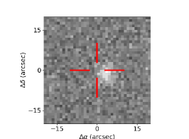
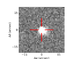
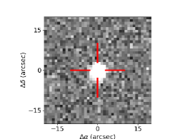
(a) Brighter fake transient

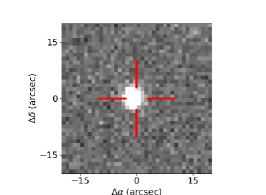
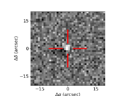
(b) Dimmer fake transient

Figure 1: An example of an injected transient and the corresponding difference image thumbnail obtained after the image subtraction. The leftmost thumbnail (both panels) is from the original image, the middle thumbnail is a result after a transient is injected, the right thumbnail shows the difference image. The location of the cross-hair is the approximate point where the transient was injected.

The fake injections are bright stars chosen from each original image. These are objects having the following properties:

$$\begin{split}m_{*}\in[13.5,16]\quad;\quad&\texttt{CLASS\_STAR}\in[0.5,1.0]\\ \texttt{FWHM}\in[1.0,3.0]\quad;\quad&\texttt{ELLIP}\in[0.0,0.3].\end{split}$$ (1)

Here $m_{*}$ is the apparent magnitude, CLASS_STAR is a quantity having a value between 0 (not star-like) and 1 (star like). FWHM is the full width at half maximum, in pixels. ELLIP is the ellipticity of the object. These quantities are reported after running SExtractor (Bertin, E. & Arnouts, S., 1996) on the original images. Objects falling in a 50 pixel wide edge boundary are left out since they could potentially be affected by image subtraction artifacts.

A square of side length $\sim 9$ arc seconds , centered around the star and local-background subtracted, constitutes a stamp. A stamp containing any other object apart from the source star is avoided. The local-background refers to that reported by SExtractor. The stamp is scaled by an appropriate scaling factor to create a point source transient of desired magnitude. Each transient is allocated a host galaxy . We follow Frohmaier et al. (2017) regarding the location in the host and place our stamp at a random pixel location within a elliptical radius of 3 pixels. This value contains sufficient amount of the flux from the galaxy.

This procedure is performed on all the images in field 100019 of iPTF, ten-fold, with a total of $\approx 2.24\times 10^{6}$ injected transients. The transient magnitudes are chosen uniformly between 15th and 22nd magnitude with the constraint that the stamp is one magnitude fainter than the original star. Therefore, $m_{\text{inj}}$ follows:

$$m_{\text{inj}}\sim\begin{cases}U(15,22)&;m_{*}\in(13.5,14)\\ U(m_{*}+1,22)&;\text{otherwise}\end{cases}.$$ (2)

An example of an injected transient in a galaxy and the new object recovered by the ISP is shown in Fig. 1.

3.2 Recovery Criteria

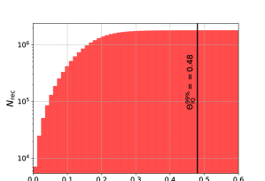
Figure 2: The figure shows the cumulative histogram of the quantity $\Theta_{\text{IQ}}$, defined as the ratio between the astronomical seeing of the image to that of the reference image as given in Eq.(4). The threshold value $\Theta^{99\%}_{\mathrm{IQ}}=0.48$ corresponds to the $99\%$ percentile. We place a constraint of this value when the objects recovered by the pipeline are spatially cross matched to an injected transient.

The recovery efficiency $\varepsilon$ is defined as the ratio of the number of injections recovered in a part of the parameter space to the total number of injections in that part. Let our injections be described by parameters $\boldsymbol{\lambda}$, then:

$$\varepsilon(\boldsymbol{\lambda})=\frac{\displaystyle N_{\text{rec}}(\boldsymbol{\lambda})\mathrm{d}\boldsymbol{\lambda}}{\displaystyle N_{\text{tot}}(\boldsymbol{\lambda})\mathrm{d}\boldsymbol{\lambda}}$$ (3)

The quantity in the numerator and denominator is the number of recovered and total injections respectively $\in\left(\boldsymbol{\lambda},\boldsymbol{\lambda}+\mathrm{d}\boldsymbol{\lambda}\right)$. Here $\boldsymbol{\lambda}$ includes both intrinsic source properties of the transient and its environment along with the observing conditions. Examples of intrinsic properties include the magnitude of the transient and the surface brightness of the host galaxy where as those for observing conditions include airmass or sky brightness. While we control fake transient brightness, the observing conditions are those of the images themselves. Since images across the full survey time are used, the parameter space of the observing conditions is automatically spanned.

We determine recovery based on the spatial cross matching of the injections with new objects reported after running the ISP. To determine the tolerance to be imposed during the cross-matching, we define $\Theta_{\text{IQ}}$ as:

$$\Theta_{\text{IQ}}=\frac{\sqrt{(x_{\text{inj}}-x_{\text{rec}})^{2}+(y_{\text{inj}}-y_{\text{rec}})^{2}}}{\Phi}$$ (4)

where $\Theta_{\text{IQ}}$ is the distance between the injected and the recovered sources in units of the seeing, $\Phi$.

We choose the threshold of $\Theta_{\text{IQ}}$ such that $99\%$ of the found injections lie within this threshold, which has a value of $\Theta^{99\%}_{\mathrm{IQ}}=0.48$ (see Fig. 2). We also impose real-bogus score threshold, $\texttt{RB2}\geq 0.1$ on the new object. This threshold on RB2 is inspired from survey operation thresholds. Out of the $\approx 2.24\times 10^{6}$ injections, we recover $\approx 1.62\times 10^{6}$.

4 Single Epoch Detectability

In this section we discuss the results of the injection campaign mentioned in Sec. 3. We first show some of the single parameter efficiencies as a comparison with those obtained for PTF (see Fig. 5 of Frohmaier et al. (2017)). For the joint multi-dimensional detectability, our analysis differs from Frohmaier et al. (2017). We treat the problem of detecting a transient in a single epoch as a binary classification problem and use the machinery of supervised learning to predict whether a transient is detected in that epoch.

4.1 Single Parameter Efficiencies

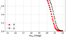
(a)

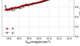
(b)

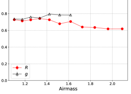
(c)

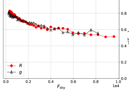
(d)

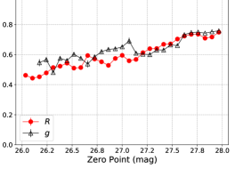
(e)

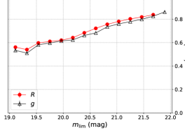
(f)

(g)

(h)

Figure 3: The single parameter efficiencies, defined in Eq. 5 are shown here. In each of the panel, the x-axis is the parameter of interest. The top two panels are parameters which are the intrinsic properties while the remaining are those taken from observing conditions. We also separate out the efficiencies based on the filter. While small deviations exists in the curves the general trend is unchanged based on the filter. Since there were more number of images (almost 3 times for field 100019) taken in R filter than g filter during iPTF survey, the range of observing conditions are larger for the R filter.

The single parameter efficiency is the marginalized version of Eq. (3). Suppose our parameter of interest is $\theta$ and the other “nuisance” parameters are given by $\boldsymbol{\gamma}$, such that in Eq. (3), $\boldsymbol{\lambda}=\{\theta,\boldsymbol{\gamma}\}$. The single parameter efficiency is:

$$\varepsilon(\theta)=\frac{\displaystyle\left[\int_{\boldsymbol{\gamma}}N_{\text{rec}}(\theta,\boldsymbol{\gamma})\mathrm{d}\boldsymbol{\gamma}\right]\mathrm{d}\theta}{\displaystyle\left[\int_{\boldsymbol{\gamma}}N_{\text{tot}}(\theta,\boldsymbol{\gamma})\mathrm{d}\boldsymbol{\gamma}\right]\mathrm{d}\theta}$$ (5)

In Fig. 3 we show the single parameter efficiencies. The expected trend of missing transients is seen in the plot for $m_{\text{inj}}$. We find that the recovery efficiency starts to drop for transients by the 20th magnitude and sensitivity is almost nil by the 22nd magnitude.

4.2 Multi-dimensional Detectability

In this section, we make a selection of parameters from the full parameter set, $\boldsymbol{\lambda}$, to those on which the detectability depends strongly. In other words, the detectability is a multi-variate function of all the possible parameters which influences the detection of a transient. We identify the minimal set which captures maximum variability. There can be correlations among a pair of parameters. For example, the sky-brightness, $F_{\text{sky}}$ and the limiting magnitude, $m_{\text{lim}}$, are correlated - a bright sky hinders the depth and results in a low value of limiting magnitude. The variation of the marginalized efficiencies shown in Fig. 3 assist us with the choice of such a parameter set. Since the trend in the single parameter efficiencies are similar to those from PTF, we select the parameters considered by Frohmaier et al. (2017) with a minor difference in the usage of the galaxy surface brightness directly, as used in Frohmaier et al. (2018), in place of the $F_{\mathrm{box}}$ parameter used in the former. This is justified because our fakes were injected in galaxies.

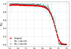
Figure 4: Comparison between single parameter efficiency of transient brightness as predicted by trained single-epoch classifier in Eq. (7) versus the distribution obtained from the ISP. The original curve has $\sim 10^{6}$ points used to train the classifier. The ML curves are made by binning the predictions made by the single-epoch classifier on a few thousand random points sampled from the parameter space of the injections (see Eq. (6)). Two cases for $10^{3}$ and $10^{4}$ points are shown. We see that the behavior of the classifier converges to that of the ISP within a small sample size ($\lesssim 1\%$ compared to the size of original distribution; see Appendix A for other parameters)

Training $\%$	Testing $\%$	Avg. mis-classification
75 $\%$	25 $\%$	5.776 $\%$
80 $\%$	20 $\%$	5.760 $\%$
85 $\%$	15 $\%$	5.745 $\%$
90 $\%$	10 $\%$	5.758 $\%$

Table 1: The table shows the average misclassification obtained for the KNearestNeighbor classifier. The complete dataset contains $\approx 2.24\times 10^{6}$ fake point source injections of which $\approx 1.62\times 10^{6}$ ($\approx 6.2\times 10^{5}$) are found (missed) by the ISP. This is split into respective training and testing fractions. The right-most column shows the fraction of the testing set for which the predictions made by the classifier, trained on the corresponding training fraction differed from the actual value. The misclassification does not change significantly as the size of training data is varied and is attributed mostly to systematics. We quote a conservative value of $6\%$ as the systematic uncertainty of the classifier.

We choose, the following set to represent the dependence of detectability:

$$\boldsymbol{\beta}=\{m,S_{\text{gal}},F_{\text{sky}},\Phi_{\text{IQ}},m_{\text{lim}}\}.$$ (6)

Here $m$ is the apparent magnitude of the transient, $S_{\text{gal}}$ is the host galaxy surface brightness, $F_{\text{sky}}$ is the sky brightness, $\Phi_{\text{IQ}}$ is the ratio of the astronomical seeing to that of the reference image and $m_{\text{lim}}$ is the limiting magnitude. The quantities $m$ and $S_{\text{gal}}$ are natural in capturing detectability. Sky brightness affects the detectability in a strong way, as is apparent from Fig. 3. The $\Phi_{\text{IQ}}$ parameter captures the variability of the atmosphere. Finally, the limiting magnitude, $m_{\text{lim}}$, although correlated with $F_{\text{sky}}$, captures longer exposure times and status of instrument electronics.

With this set, we use the machinery of supervised learning provided by the scikit-learn library (Pedregosa et al., 2011) to train a binary classifier based on the results of the ISP. Once trained, the classifier outputs a probability of detection given arbitrary but physical values of $\boldsymbol{\beta}$. We denote this trained classifier by $\hat{\varepsilon}$:

$$\hat{\varepsilon}=\hat{\varepsilon}(m,S_{\text{gal}},F_{\text{sky}},\Phi_{\text{IQ}},m_{\text{lim}}).$$ (7)

The scikit-learn library provides a suite of classifiers. We choose the non-parametric KNearestNeighbor classifier based on speed and accuracy given our large volume of training data. We train the classifier using 11 neighbors - twice the number of dimensions plus one to break ties. The observation of a fiducial transient is a point in this parameter space. To decide if that point is “missed” or “found”, we use a majority vote from the nearest 11 neighbors. We checked that increasing the number of neighbors does not significantly increase the correctness of predictions made by the classifier. We note that one could use a different threshold for this classification. For example, a different option could be to use greater than 3 “found” neighbors to call the arbitrary point as found. However, it comes at a cost of misclassification. From the predictions of the classifier on the testing set, we find the systematic uncertainty of the classifier to be $\approx 6\%$ i.e. 6 out of 100 predictions made by the classifier is expected to be either true negative or false positive cases. The result does not change much if the size of the training and testing set is varied . A comparison between the predictions made by the trained classifier and the original ISP efficiency with the transient magnitude is presented in Fig. 4. We see that the behavior of the ISP is reproduced by feeding the classifier with only a few thousand points randomly chosen from the parameter space.

5 Lightcurve Recovery

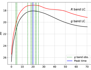
Figure 5: Upper panel: An example of a SALT2 lightcurve, with the apparent magnitude, $m$ on the y-axis and time on the x-axis. The lightcurves in the iPTF $R$ and $g$ bands are shown. The observations of the telescope are shown as vertical lines. At each observation, we also have the observing conditions of the telescope from archival data. Lower panel: The same lightcurve is plotted, however, the vertical lines now represent the detectability from the single epoch classifier. Based on the criteria of confirming a lightcurve as SN Ia, this lightcurve was recovered.

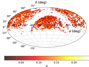
Figure 6: An ensemble of SN Ia lightcurves were simulated out to a redshift, $z_{\mathrm{max}}^{\mathrm{Ia}}=0.28$, uniform in co-moving volume. This figure shows the distribution of the recovered SN Ia in the sky colored by the redshift. The galactic plane can be seen as the half annulus region with no detections.

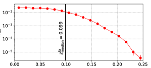
Figure 7: Recovery efficiency of the SN Ia lightcurves as a function of redshift, $z$. The median volume weighted redshift is found to be $z_{\text{median}}^{\text{Ia}}=0.099$.

In this section, we assess the detectability of lightcurves using SNe Ia as our case study. We simulate lightcurves with varying intrinsic properties, sky location and redshift, and use the single epoch detectability classifier mentioned in Eq. (7) together with the observing schedule of iPTF to determine their sensitivity. The steps are as follows:

1. We simulate lightcurves of varying intrinsic properties over space-time.

2. From the complete iPTF observing schedule, we determine the observations of the evolving lightcurve. This depends on the duty cycle of the instrument. On extended periods with no observations, the simulated lightcurves are missed.

3. We associate a host galaxy with the supernova by choosing a surface brightness value from the distribution of galaxy surface brightness in the survey.

4. Every time the transient is “seen” by iPTF , we feed the combination of the apparent magnitude, host galaxy surface brightness along with the observing conditions at that epoch to the trained single epoch classifier developed in Sec.  4. This step, in a sense, mimics the action of the ISP.

5. We call the lightcurve recovered when we have at least 5 found observations, all brighter than 20th magnitude, with a minimum of 2 observations on the lightcurve rise and a minimum of 2 on the fall. This is motivated by survey time discoveries.

We also consider type II supernova lightcurves for comparison. Type II supernovae are complex and are further categorized into different subtypes. We consider the IIp subtype because compared to the $\sim$ weeks long variability of SNe Ia, IIp lightcurves vary $\sim 100$ days and hence is a complimentary case to study. The analysis for the IIps, however, is simpler compared to Ias.

5.1 SN Ia Lightcurves

We use SN Ia lightcurves from the SALT2 model (Guy et al., 2007). In particular, we use the Python implementation of SALT2 provided in sncosmo library (Barbary, 2014). This model is based on observations of SNe Ia by the SDSS and SNLS surveys. The free parameters of the model include the stretch ($x_{1}$) and color ($C$) parameters of the SN Ia. Regarding the range of these parameters, we follow same range as Frohmaier et al. (2017) (see Table 1 and Eq.(4) therein). The ranges cover the possible lightcurve morphologies of SNe Ia (Betoule et al., 2014). We show an example lightcurve, at a redshift of $z=0.01$ with an instrinsic $M_{B}=-19.05$ in Fig. 5. When propagating the flux, we also take into account the extinction due to host galaxy dust and the Milky Way (MW) dust. We use the MW dust map by Fitzpatrick (1999) which is a part of the sncosmo package. For the host galaxy extinction, we use the distribution of $E(B-V)$ of SN Ia in their host galaxies (Hatano et al., 1998). Dust extinction plays a significant role in the detectability of lightcurves as the SNe can be dimmed by as much as $1-1.5$ magnitudes.

5.2 Lightcurve Ensemble

We simulate $\approx 5\times 10^{6}$ SN Ia lightcurves uniformly in co-moving volume up to redshift, $z_{\mathrm{max}}^{\mathrm{Ia}}=0.28$ , uniform in peak time distribution in the observer frame. We assume a flat $\Lambda\mathrm{CDM}$ cosmology with Hubble constant, $H_{0}=69.3$ $\mathrm{kms^{-1}/Mpc}$ and matter to critical density, $\Omega_{\mathrm{m}}=0.287$ . We associate a host galaxy surface brightness to each of these SNe using the distribution of surface brightness from iPTF data.

The epochs when the SN Ia is observed come from the iPTF observing schedule. At each observation, we obtain the transient magnitude at that epoch from the lightcurve and the observing conditions from the iPTF survey database. The single epoch classifier then tells us the epochs when the transient was detected. An example is shown in Fig. 5 where the vertical lines in the upper and lower panel respectively represent the observations and detections at each epoch.

5.3 SN Ia Space-time Sensitive Volume

To understand rates, one must have a good estimate of the survey sensitivity to particular transient types. Let $\Lambda_{\text{SNe}}$ be the expected count of SNe seen during survey time. Then, with $R$ as the intrinsic rate we have:

$$\Lambda_{\text{SNe}} = \int f(t;\underbrace{M_{B},z,\dots}_{\boldsymbol{\kappa}})\overbrace{\frac{\mathrm{d}N}{\mathrm{d}t_{e}\mathrm{d}V_{c}}}^{R}\frac{1}{1+z}\frac{\mathrm{d}V_{c}}{\mathrm{d}z}\mathrm{d}z\mathrm{d}t\mathrm{d}\boldsymbol{\kappa}$$

$$= R\int f(t;\underbrace{M_{B},z,\dots}_{\boldsymbol{\kappa}})\frac{1}{1+z}\frac{\mathrm{d}V_{c}}{\mathrm{d}z}\mathrm{d}z\mathrm{d}t\mathrm{d}\boldsymbol{\kappa}$$

$$= R\langle VT\rangle,$$

where the integral runs over time of observation and co-moving volume up to $z_{\mathrm{max}}^{\mathrm{Ia}}=0.28$. The selection function, $f(\dots)\in\{0,1\}$, is to be interpreted as the weight assigned to regions in space-time. The value of the selection function is a consequence of running a particular instance of SN Ia through the observing schedule and inferring detectability based on the single-epoch classifier in Eq. (7). Therefore, the selection function depends on the observer time, $t$, which captures the duty cycle and cadence. Also, it depends on the intrinsic properties of the supernova like the absolute intrinsic magnitude, $M_{B}$, the redshift, $z$, at which it was simulated, the sky location and so on. These are collectively represented by $\boldsymbol{\kappa}$ in Eq. (5.3). Since we have distributed the supernovae uniformly in co-moving volume, the integral is approximated in the Monte-Carlo sense:

$$\langle VT\rangle = \int f(t;\underbrace{M_{B},z,\dots}_{\boldsymbol{\kappa}})\frac{1}{1+z}\frac{\mathrm{d}V_{c}}{\mathrm{d}z}\mathrm{d}z\mathrm{d}t\mathrm{d}\boldsymbol{\kappa}$$ (9)

$$\approx \frac{N_{\text{rec}}}{N_{\text{tot}}}T\int\frac{1}{1+z}\frac{\mathrm{d}V_{c}}{\mathrm{d}z}\mathrm{d}z,$$

where $N_{\text{rec}}$ is the number of SNe recovered from this simulation campaign, $N_{\text{tot}}$ is the total number simulated and $T$ is the four year period of iPTF over which we performed the simulations . We obtain the result:

$$\langle VT\rangle_{\mathrm{Ia}}=2.93\pm 0.21\times 10^{-2}\;\mathrm{Gpc^{3}\,yr}$$ (10)

where the error includes the $\sim 1/\sqrt{N}$ statistical error from Monte Carlo integration and the $6\%$ systematic error of the single epoch detectability classifier computed in Sec. 4.2, the latter being the dominant source of error. The distribution of the detected SNe Ia in sky is shown in Fig. 6 colored by redshift. Using the recovered SNe Ia, the median sensitive co-moving volume is found to be $0.305$ $\mathrm{Gpc^{3}}$. We report the redshift corresponding to this value as the median sensitive redshift to SNe Ia, $z_{\text{median}}^{\text{Ia}}=0.099$, shown in Fig. 7.

5.4 SN IIp Space-time Sensitive Volume

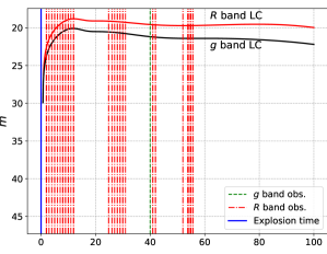
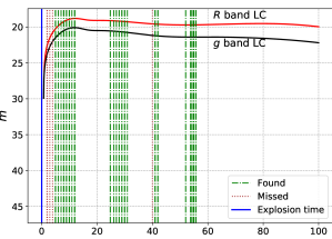
Figure 8: Upper panel: An example of a SN IIp lightcurve, with the apparent magnitude, $m$ on the y-axis and time on x-axis. The lightcurve is shown in the iPTF $R$ and $g$ bands. The observations of the telescope are shown as vertical lines. Lower panel: The same lightcurve is plotted, however, the vertical lines now represent the recovery by single epoch classifier. One can identify the only $g$ band observation (around 40 days) being missed due to fainter magnitude in the $g$ band.

In contrast to the well-defined Ia lightcurves with their typical timescales of several weeks, we also wanted to explore longer-timescale lightcurves as a limiting case. Therefore, we consider type IIp supernovae and compute their space-time sensitive volume in similar lines as Sec. 5.2. In general, type II supernovae (SNe II) vary in lightcurve morphology and are categorized in various subtypes (Li et al., 2011). Specifically, type IIp lightcurves have a distinct “plateau” feature after the rise lasting for about 100 days after explosion, as shown in Fig. 8. The intrinsic brightness, $M_{B}\sim-16.75$, is significantly lower than that of SNe Ia (Richardson et al., 2014). Hence, we expect the space-time sensitive volume to be lower than that of the SNe Ia. When considering the Ia lightcurves in Sec. 5.1, the SALT2 model parameters were used to tune possible lightcurve morphologies. Here we take a simpler approach and consider a time-series model from Gilliland et al. (1999) (named nugent-sn2p in the sncosmo package) to compute the flux up to 100 days from the explosion time. Thus, while simulating the SNe IIp in space-time, the only change to the lightcurve shape is the “stretch” depending on the cosmological redshift.

We simulate $\sim 9.1\times 10^{5}$ SN IIp lightcurves uniform in sky location, observer time and co-moving volume up to a redshift, $z=0.1$. Like the SNe Ia, each SN IIp is assigned a host galaxy surface brightness from the surface brightness distribution of galaxies in iPTF and a $E(B-V)$ extinction value from IIp extinction distribution in Hatano et al. (1998). In this case, we use the criteria that the lightcurve must be recovered a minimum of five epochs, brighter than 20th magnitude in a span of 3 weeks within the 100 days post explosion. The iPTF observing schedule along with the single-epoch classifier is used to compute the detectability in each epoch. We obtain the result:

$$\langle VT\rangle_{\mathrm{IIp}}=7.80\pm 0.76\times 10^{-4}\;\mathrm{Gpc^{3}\,yr},$$ (11)

where the error includes the statistical error from the Monte-Carlo integration and the $6\%$ systematic uncertainty from the single-epoch classifier (see Sec. 4.2). The median sensitive redshift is found to be $z_{\text{median}}^{\text{IIp}}=0.038$.

6 Discussion and Conclusions

In this work, we provide a methodology to assess the transient detectability taking into account the intrinsic transient properties and the observing conditions of fast cadence transient surveys. This is done by injecting fake point source transients into the images, running image subtraction on them and finding out the parameter space where they are found by the image subtraction pipeline. The joint detectability is evaluated using the machinery of supervised machine learning trained on the missed and found fake transients. This step mimics the action of the image subtraction pipeline at every epoch and forms the single-epoch detectability. Consequently, the lightcurve morphology and the survey observing schedule is used to compute the space-time volume sensitivity of particular transients. We consider the case of the intermediate Palomar Transient Factory (iPTF) and evaluate the single-epoch detectability and then use its observing schedule to compute the space-time volume sensitivity of type Ia supernovae (SNe Ia). We also do a preliminary analysis of type IIp supernovae (SNe IIp). Note that the space-time volume sensitivity could be computed for any general transient, using its lightcurve morphology; SN Ia or IIp is an example. In the case of SNe Ia, the remaining piece in the estimation of the volumetric rate is a systematic number count to be obtained via an archival search into iPTF data. While we defer this to a future work, we outline our plan of action here.

6.1 Rates

The computation of the rate posterior assumes the likelihood of observing $N$ candidate events is an inhomogeneous Poisson process (Loredo & Wasserman, 1995; Farr et al., 2015). Our search will filter the SN Ia population based on the model presented in Sec. 5 at the expense of some contamination from other transient types, potentially with similar lightcurve morphologies. If the mean count of these impurities is $\Lambda_{0}$, the likelihood function is:

$$p\left(N|\Lambda_{0},\Lambda_{\text{SNe}}\right)\propto\left(\Lambda_{0}p_{0}+\Lambda_{\text{SNe}}p_{\text{SNe}}\right)^{N}$$

$$\times\exp{\left(-\Lambda_{0}-\Lambda_{\text{SNe}}\right)},$$ (12)

where $p_{\text{SNe}}$ ($p_{0}$) is the a priori weight that a transient is (isn’t) a SN Ia after the filtering process. With a suitable choice of prior, we can use Bayes’ theorem to obtain the posterior. Considering the Jeffreys’ prior:

$$p\left(\Lambda_{0},\Lambda_{\text{SNe}}\right)=\frac{1}{\sqrt{\Lambda_{0}}}\frac{1}{\sqrt{\Lambda_{\text{SNe}}}},$$ (13)

the posterior takes the form:

$$p\left(\Lambda_{0},\Lambda_{\text{SNe}}\right|N) \propto p\left(N|\Lambda_{0},\Lambda_{\text{SNe}}\right)p\left(\Lambda_{0},\Lambda_{\text{SNe}}\right)$$ (14)

$$\propto \frac{\left(\Lambda_{0}p_{0}+\Lambda_{\text{SNe}}p_{\text{SNe}}\right)^{N}}{\sqrt{\Lambda_{0}\Lambda_{\text{SNe}}}}$$

$$\times\exp{\left(-\Lambda_{0}-\Lambda_{\text{SNe}}\right)}.$$

Integrating out the nuisance parameter, $\Lambda_{0}$, we have the marginalized posterior on $\Lambda_{\text{SNe}}=R\langle VT\rangle$, or equivalently on $R$:

$$p\left(R|N\right) = \int_{0}^{\infty}p\left(\Lambda_{0},\Lambda_{\text{SNe}}\right|N)\mathrm{d}\Lambda_{0}$$ (15)

$$\propto \frac{e^{-R\langle VT\rangle}}{\sqrt{R\langle VT\rangle}}\times\left[\left(R\langle VT\rangle p_{\text{SNe}}\right)^{N}+\right.$$

$$\left.\frac{N}{2}p_{0}\left(R\langle VT\rangle p_{\text{SNe}}\right)^{N-1}\right],$$

where we expand Eq. (14) and integrate, keeping terms up to linear order in $p_{0}$ since we expect that $p_{0}\ll p_{\text{SNe}}$.

6.2 Approximate SN Ia Count in iPTF

Type Ia supernova rates have been studied earlier in the literature (Dilday et al., 2008; Gal-Yam et al., 2007; Brown et al., 2019). Deep field instruments have provided estimates of the Ia rate out to high redshift (Gal-Yam et al., 2007). The intermediate Palomar Transient Factory, being an all sky survey has a comparatively lower sensitivity to SNe Ia at $z_{\text{median}}^{\text{Ia}}=0.099$, evaluated in Sec. 5. The SDSS-II supernova survey has estimated the volumetric SN Ia rate at $z\approx 0.1$ to be $R_{\mathrm{SNIa}}^{\mathrm{SDSS-II}}\sim 2.9^{+1.07}_{-0.75}\times 10^{-5}\mathrm{Mpc^{-3}yr^{-1}}$ (Dilday et al., 2008). Using our estimate of the space-time sensitive volume from Eq. (10), an estimate of the count of SNe Ia in iPTF is $630-1160$. This is consistent with $1035$ objects tagged “SN Ia” during the survey time.

6.3 Future Work

While the number of transients tagged as “SN Ia” by human scanners during iPTF survey time seem consistent with our ballpark above, the systematic uncertainty of such a classification remains unquantified. The quantities $p_{0}$, $p_{\text{SNe}}$ and $N$ in Eq. (15) require a systematic search into the iPTF archival data to retrieve the candidate count and systematic errors associated with such a classification. We defer this and the computation of SN Ia volumetric rate to a future work in the series.

The methodology developed here facilitates the computation of space-time volume sensitivities of general transient types. Of particular interest are the fast transients in iPTF archival data as discussed in Ho et al. (2018). Also, the observation of the “kilonova” resulting from the binary neutron star merger, GW170817 (Abbott et al., 2017, 2017a, 2017b), hints towards the association of transients to binary neutron star mergers. There is no evidence of detection of such a transient in the iPTF data, in which case rate upper limits could be placed due to non-detection.

Appendix A Classifier Single-epoch performance

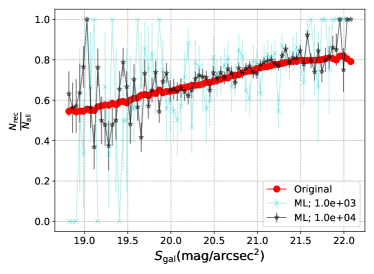
(a)

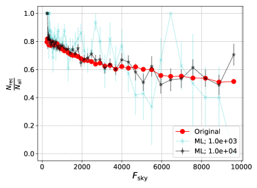
(b)

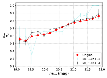
(c)

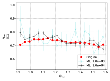
(d)

Figure 9: This figure is an extension of Fig. 4. We compare the performance of the marginalized single parameter efficiency of the trained classifier compared to that of the original distributions in Fig. 3. We see the behavior of the ISP being reproduced by feeding the classifier a few thousand points.

In Fig. 4, we made a comparison between the marginalized single parameter efficiency for the single-epoch transient brightness from the classifier predictions. Here, we show it for the remaining parameters. While the final classifier is trained on the full dataset, to make the comparison, we train it on $90\%$ of the total fake point source simulations we performed, as mentioned in Sec. 3.1. From the remaining $10\%$ sample size, we make a random selection of points (progressively increasing), feed them to the classifier and bin the results in the same manner as in Fig. 3 to compare marginalized efficiency plots. These are shown in Fig. 9 and Fig. 4, the latter presented earlier. We see that the behavior starts to converge to that of the ISP in a few thousand points.

References

- Abbott et al. (2017a) Abbott, B. P., et al. 2017a, The Astrophysical Journal, 850, L39
- Abbott et al. (2017b) —. 2017b, The Astrophysical Journal, 848, L13
- Abbott et al. (2017) Abbott, B. P., Abbott, R., Abbott, T. D., et al. 2017, ApJ Lett., 848, L12
- Astropy Collaboration et al. (2018) Astropy Collaboration, Price-Whelan, A. M., Sipőcz, B. M., et al. 2018, AJ, 156, 123
- Barbary (2014) Barbary, K. 2014, doi:10.5281/zenodo.11938
- Becker (2015) Becker, A. 2015, HOTPANTS: High Order Transform of PSF ANd Template Subtraction, , , ascl:1504.004
- Bertin, E. & Arnouts, S. (1996) Bertin, E., & Arnouts, S. 1996, Astron. Astrophys. Suppl. Ser., 117, 393
- Betoule et al. (2014) Betoule, M., Kessler, R., Guy, J., et al. 2014, A&A, 568, A22
- Bloom et al. (2013) Bloom, J. S., Brink, H., Richards, J. W., et al. 2013, Monthly Notices of the Royal Astronomical Society, 435, 1047
- Brown et al. (2019) Brown, J. S., Kochanek, C. S., Stanek, K. Z., et al. 2019, Monthly Notices of the Royal Astronomical Society, 484, 3785
- Cao et al. (2016) Cao, Y., Nugent, P. E., & Kasliwal, M. M. 2016, Publications of the Astronomical Society of the Pacific, 128, 114502
- Dilday et al. (2008) Dilday, B., Kessler, R., Frieman, J. A., et al. 2008, The Astrophysical Journal, 682, 262
- Drake et al. (2009) Drake, A. J., Djorgovski, S. G., Mahabal, A., et al. 2009, The Astrophysical Journal, 696, 870
- Farr et al. (2015) Farr, W. M., Gair, J. R., Mandel, I., & Cutler, C. 2015, Phys. Rev. D, 91, 023005
- Fitzpatrick (1999) Fitzpatrick, E. L. 1999, Publications of the Astronomical Society of the Pacific, 111, 63
- Frohmaier et al. (2018) Frohmaier, C., Sullivan, M., Maguire, K., & Nugent, P. 2018, The Astrophysical Journal, 858, 50
- Frohmaier et al. (2017) Frohmaier, C., Sullivan, M., Nugent, P. E., Goldstein, D. A., & DeRose, J. 2017, The Astrophysical Journal Supplement Series, 230, 4
- Gal-Yam et al. (2007) Gal-Yam, A., Filippenko, A. V., Jannuzi, B. T., et al. 2007, Monthly Notices of the Royal Astronomical Society, 382, 1169
- Gilliland et al. (1999) Gilliland, R. L., Nugent, P. E., & Phillips, M. M. 1999, ApJ, 521, 30
- Guy et al. (2007) Guy, J., Astier, P., Baumont, S., et al. 2007, Astronomy & Astrophysics, 466, 11
- Hatano et al. (1998) Hatano, K., Branch, D., & Deaton, J. 1998, The Astrophysical Journal, 502, 177
- Hinshaw et al. (2013) Hinshaw, G., Larson, D., Komatsu, E., et al. 2013, ApJS, 208, 19
- Ho et al. (2018) Ho, A. Y. Q., Kulkarni, S. R., Nugent, P. E., et al. 2018, The Astrophysical Journal, 854, L13
- Holoien et al. (2019) Holoien, T. W.-S., Brown, J. S., Vallely, P. J., et al. 2019, MNRAS, 484, 1899
- Hunter (2007) Hunter, J. D. 2007, Computing In Science & Engineering, 9, 90
- Ivezić et al. (2008) Ivezić, Ž., Kahn, S. M., Tyson, J. A., et al. 2008, arXiv e-prints, arXiv:0805.2366
- Jones et al. (2001–) Jones, E., Oliphant, T., Peterson, P., et al. 2001–, SciPy: Open source scientific tools for Python, , , [Online; accessed ¡today¿]
- Kaiser et al. (2010) Kaiser, N., Burgett, W., Chambers, K., et al. 2010, The Pan-STARRS wide-field optical/NIR imaging survey, , , doi:10.1117/12.859188
- Kulkarni (2016) Kulkarni, S. R. 2016, in American Astronomical Society Meeting Abstracts, Vol. 227, American Astronomical Society Meeting Abstracts #227, 314.01
- Law et al. (2009) Law, N. M., Kulkarni, S. R., Dekany, R. G., et al. 2009, Publications of the Astronomical Society of the Pacific, 121, 1395
- Li et al. (2011) Li, W., Chornock, R., Leaman, J., et al. 2011, MNRAS, 412, 1473
- Loredo & Wasserman (1995) Loredo, T. J., & Wasserman, I. M. 1995, ApJS, 96, 261
- Maoz & Mannucci (2012) Maoz, D., & Mannucci, F. 2012, PASA, 29, 447
- McKinney (2010) McKinney, W. 2010, in Proceedings of the 9th Python in Science Conference, ed. S. van der Walt & J. Millman, 51 – 56
- Nugent et al. (2015) Nugent, P., Cao, Y., & Kasliwal, M. 2015, The Palomar transient factory, , , doi:10.1117/12.2085383
- Pedregosa et al. (2011) Pedregosa, F., Varoquaux, G., Gramfort, A., et al. 2011, Journal of Machine Learning Research, 12, 2825
- Richardson et al. (2014) Richardson, D., Jenkins, Robert L., I., Wright, J., & Maddox, L. 2014, AJ, 147, 118
- Sako et al. (2007) Sako, M., Bassett, B., Becker, A., et al. 2007, The Astronomical Journal, 135, 348
- Shanks et al. (2015) Shanks, T., Metcalfe, N., Chehade, B., et al. 2015, MNRAS, 451, 4238
- van der Walt et al. (2011) van der Walt, S., Colbert, S. C., & Varoquaux, G. 2011, Computing in Science Engineering, 13, 22