Quantum chromodynamics axion in a hot and magnetized medium

Abstract

It is analyzed the effects of a hot and magnetized medium on the axion mass, self-coupling and topological susceptibility when in presence of an anisotropic external magnetic field along the $z$-direction, within the Nambu–Jona-Lasinio effective model for quantum chromodynamics. The effects of both Magnetic Catalysis and Inverse Magnetic Catalysis are explicitly taken into account through appropriate matching of parameters with those from lattice Monte-Carlo numerical simulations. It is also analyzed the dependence of the results with respect to different model parametrizations in the context of the Nambu–Jona-Lasinio model.

I Introduction

The axion is a pseudo Nambu-Goldstone boson of a spontaneously broken global Abelian symmetry Peccei:1977hh . The axion is considered to be the most elegant and robust solution to the absence of the charge and parity (CP) violating effects (also dubbed the strong CP problem) in quantum chromodynamics (QCD) Weinberg:1977ma ; Wilczek:1977pj . It has also been considered as a prime candidate for cold dark matter given that they are very weakly coupled to baryonic matter in general, besides of possibly being extremely light (see, e.g., Ref. Marsh:2015xka for a recent review and references therein).

The importance of the QCD axion as a solution to the strong CP problem and its potential in explaining the dark matter abundance in the universe makes it one of the most sought out prospects beyond the particle physics Standard Model. Recent studies also show that axions can thermalize and form a Bose-Einstein condensate Sikivie:2009qn ; Chavanis:2017loo which in turn indicates the relevance of finite temperature extension of the axion properties. On the other hand, the coupling of QCD axions with an external electromagnetic field was first exploited long ago in Ref. Sikivie:1983ip to make the axion experimentally detectable. Since then various other experimental techniques involving the axion-photon coupling have been proposed Sikivie:1985yu ; VanBibber:1987rq ; DePanfilis:1987dk and results of some such experiments are also available Hagmann:1990tj ; Sikivie:1993jm .

Axions have also been associated with the anomalous stellar cooling problem Raffelt:2006cw ; Giannotti:2015kwo , including neutron stars as1 ; as2 ; as3 . This is because axions could be produced in hot astrophysical plasmas and, thus, could take part of the energy transport in stellar objects. This is in particular a motivation for studying the properties of the QCD axion when in presence of an environment that accounts not only thermal effects (which can also be of relevance to the physics of these particles in the early universe), but also density (chemical potential) and external magnetic fields (relevant also for the physics of compact stellar objects, like neutron stars).

As a pseudo Goldstone boson, the QCD axion acquires a mass, $m_{a}$, from the QCD chiral symmetry breaking and this mass is typically of $\mathcal{O}(m_{\pi}f_{\pi}/f_{a})$ Weinberg:1977ma , where $m_{\pi}$ is the pion mass, $f_{\pi}$ is the pion decay constant and $f_{a}$ is the axion decay constant, which is proportional to the Peccei-Quinn symmetry breaking scale. We can also define an effective self-coupling, $\lambda_{a}$, to the axion field. Furthermore, there are derivative couplings that can also be present in a system involving axions. The axion mass and the couplings (including the self-coupling) are all controlled by the scale $f_{a}$. Though exact determination of the value of $f_{a}$ is not yet achievable, present astrophysical constraints suggest the value for $f_{a}$ to be in between $10^{8}$ GeV and $10^{18}$ GeV Raffelt:2006cw ; Arvanitaki:2010sy ; Arvanitaki:2014wva . This makes the couplings associated with axion field extremely small, making it experimentally challenging to be probed (see, e.g., Ref. Brun:2019lyf and references therein for some of the experimental proposals looking for axions).

The extension of axion studies in relatively higher temperatures can be done perturbatively, using, e.g., the dilute instanton gas approximation Turner:1985si . But around and below the pseudo critical temperature, $T_{c}\sim 170$ MeV, which are particularly important in relation with the chiral symmetry breaking, there are no reliable perturbative techniques. Non-perturbative methods making use of effective models come into play in this regime of study along with the first principle calculations of Lattice QCD. In this particular work, we have chosen to deal with one of such effective model, the Nambu–Jona-Lasinio (NJL) model Klevansky:1992qe to study the QCD axions in a hot and magnetized medium (For a recent study of axion within a chiral effective Lagrangian model, see Ref Landini:2019eck ). Beside its relevance to spontaneous CP violation Frank:2003ve ; Boomsma:2009eh ; Boomsma:2009yk ; Chatterjee:2014csa ; Fukushima:2001hr , the advantage of using a two-flavor NJL model to study a system of axions is that being a quark model, it incorporates the effects of axions via the effective (‘t Hooft determinant) interaction tHooft:1976snw ; tHooft:1986ooh . As for the electromagnetic coupling of the axions, for this work we will only consider an anisotropic external magnetic field along the $z$-direction. In the future we plan to extend the present study for other general systems, where both electric and magnetic fields can be present in the system. As an additional remark, since the energy scales we are working with are much smaller than the axion symmetry breaking scale $f_{a}$, we can consider the axion field to be in its (constant) vacuum expectation value, so it behaves like a CP violating term added to the QCD action. Thus, in this sense, our derivations can be performed in a way similar like in previous studies Frank:2003ve ; Boomsma:2009eh ; Boomsma:2009yk ; Chatterjee:2014csa ; Fukushima:2001hr .

This paper is organized as follows. In Sec. II we discuss the formalism of the NJL model when incorporating the axion field. We also explain the derivation of the thermodynamic potential for the model in the cases without and with an external anisotropic magnetic field. The way the parameters are fixed is also discussed. In Sec. III we present our results concerning the analysis of the effects of temperature and magnetic field on the axion mass, coupling constant and also on the axion topological susceptibility, which is an important observable derivable for example from lattice QCD results. Finally, in Sec. IV we have our conclusions.

II Formalism

We start with a brief review of the QCD axion and how its associated field is included in the NJL model quasi-particle description of quark matter. Then, we will discuss the incorporation of both temperature and an external anisotropic magnetic field in the derivation of the thermodynamic potential for the model. While parametrizing the model, focus will also be given on the recently discovered phenomena of Magnetic Catalysis (MC) Gusynin:1995nb and Inverse Magnetic Catalysis (IMC) Bali:2011qj ; Bali:2012zg on the thermodynamic potential when in presence of a magnetized medium.

II.1 The axion contribution

The study of CP violation within strongly interacting matter has been a subject of extensive scrutiny over the years Frank:2003ve ; Boomsma:2009eh ; Boomsma:2009yk ; Chatterjee:2014csa ; Fukushima:2001hr ; Fraga:2009vy ; Mizher:2008hf ; Mizher:2008dj ; Fraga:2008um . It is a well known fact that within the regime of strong interaction instanton contributions can lead to CP violation tHooft:1976snw ; tHooft:1986ooh . In this kind of scenarios where gauge field configurations have nontrivial topologies, the QCD Lagrangian density generally contains an extra $\theta$-term,

$$\mathcal{L}_{\theta}=\frac{\theta g^{2}}{32\pi^{2}}\mathcal{F}\bar{\mathcal{F}},$$ (1)

where $g$ is the coupling for the strong interaction and $\mathcal{F}$ and $\bar{\mathcal{F}}$ are the gluonic field strength tensor and its dual respectively. The real parameter $\theta$ defines the choice of vacuum from infinite possibilities and its value subsequently dictates whether the corresponding theory is CP symmetric or not. As can be seen straightforwardly from Eq. (1), only for $\theta=0$ (mod $\pi$), the QCD Lagrangian is CP conserving. Again various experimental studies on pseudoscalar mass ratios Kawarabayashi:1980uh , electrical dipole moments Baluni:1978rf ; Crewther:1979pi ; Baker:2006ts ; Afach:2015sja as well as Lattice QCD calculations Guo:2015tla ; Bhattacharya:2015esa conclude that the value of this real angular parameter $\theta$ is very close to 0 in nature. A simple and elegant way to explain why $\theta$ should be so small or null is giving $\theta$ a dynamical character, elevating it to a field, the axion, such as to have a vanishing vacuum expectation value Peccei:1977hh . The axion field $a$ is the canonically normalized dynamical $\theta$, $\theta(x)=a(x)/f_{a}$, where $f_{a}$ is the axion decay constant. Its only non-derivative coupling is to the QCD topological charge and it is suppressed by the scale $f_{a}$. The interaction Lagrangian density in Eq. (1) can now be written as

$$\mathcal{L}_{a}=\frac{g^{2}}{32\pi^{2}}\frac{a}{f_{a}}\mathcal{F}\bar{\mathcal{F}}.$$ (2)

Equation (2) can be effectively represented as an interaction of the QCD axion field $a$ with the quarks by performing a chiral rotation Buballa:2003qv of the quark fields by the angle $a/f_{a}$, which yields tHooft:1976snw ; tHooft:1986ooh

$$\mathcal{L}_{a}=8G_{2}\left[e^{i\frac{a}{f_{a}}}\text{det}(\psi_{R}\psi_{L})+e^{-i\frac{a}{f_{a}}}\text{det}(\psi_{L}\psi_{R})\right],$$ (3)

where $\psi_{L}$ and $\psi_{R}$ are the left- and right-handed components of the quark wave function $\psi$ and $G_{2}$ is a coupling constant.

II.2 Thermodynamic potential for the axion background field within the NJL model

The effective Lagrangian density for the isospin symmetric two-flavor NJL model with the CP violating term is given by

$$\mathcal{L}=\bar{\psi}(i\gamma^{\mu}\partial_{\mu}-m_{0})\psi+\mathcal{L}_{q}+\mathcal{L}_{a},$$ (4)

where $\psi$ depicts the fermionic (quark) fields and $m_{0}$ is the current quark mass. The fermionic interaction part of the Lagrangian density is given by

$$\mathcal{L}_{q}=G_{1}\left[(\bar{\psi}\psi)^{2}+(\bar{\psi}\tau_{k}i\gamma_{5}\psi)^{2}\right],$$ (5)

where $\tau_{k}$, $k=0,1,2,3$, represents the unit matrix (for $k=0$) and the Pauli matrices (for $k=1,2,3$) and $G_{1}$ is the coupling constant associated with the fermionic interaction. Lastly, the symmetry breaking ’t Hooft determinant interaction term ${\cal L}_{a}$ is given by Eq. (3). The axion contribution Eq. (3) effectively breaks down the global U$(2)_{V}$ symmetry into SU$(2)_{V}\times$ U$(1)_{B}$. Often, in recent studies involving flavor mixing within the NJL model and its extensions, the couplings $G_{1}$ and $G_{2}$ are also taken to be equal Frank:2003ve ; Buballa:2003qv . In the present work we choose $G_{1}=(1-c)G_{s}$ and $G_{2}=c\,G_{s}$, following Refs. Frank:2003ve ; Boomsma:2009eh ; Lu:2018ukl , which assumes the connection of both the coupling constants with $G_{s}$, the standard scalar channel coupling constant for the NJL model. The parameter $c$ connecting the two couplings determines the strength of the axion interaction and we will discuss more about its value in Section II.4.

Next, for the derivation of the thermodynamic potential, we use the usual mean-field approximation Klevansky:1992qe , where the scalar and pseudoscalar fields are replaced by their corresponding mean-field values, or condensates,

$$\bar{\psi}\psi\rightarrow\langle\bar{\psi}\psi\rangle=\sigma,$$ (6)

$$\bar{\psi}i\gamma_{5}\psi\rightarrow\langle\bar{\psi}i\gamma_{5}\psi\rangle=\eta,$$ (7)

with $\sigma$ and $\eta$ representing the chiral and pseudoscalar condensates, respectively. Note that in the following we will be considering only the isospin symmetric case, hence, only $\langle\bar{\psi}\psi\rangle$ and $\langle\bar{\psi}i\gamma_{5}\psi\rangle$ survive from Eq. (5). Usually, for $\theta=0$, or in the present case, for $a=0$, $\langle\bar{\psi}i\gamma_{5}\psi\rangle$ also vanishes. Considering a nonvanishing $\langle\bar{\psi}i\gamma_{5}\psi\rangle$ emphasizes explicitly the fact that the axion field couples to the axial current. Hence, in terms of $\sigma$ and $\eta$, the thermodynamic potential for the QCD axion within the NJL model, following for instance Ref. Lu:2018ukl , is given by

$$\Omega = \Omega_{q}+G_{1}(\eta^{2}+\sigma^{2})-G_{2}(\eta^{2}-\sigma^{2})\cos\frac{a}{f_{a}}$$ (8)

$$-2G_{2}\sigma\eta\sin\frac{a}{f_{a}},$$

where the quark contribution $\Omega_{q}$ is given by Klevansky:1992qe ; Buballa:2003qv

$$\Omega_{q}=-8N_{c}\int\frac{d^{3}p}{(2\pi)^{3}}\left[\frac{E_{p}}{2}+T\ln\left(1+e^{-E_{p}/T}\right)\right],$$ (9)

where $N_{c}=3$ is the number of colors, $E_{p}=\sqrt{p^{2}+M^{2}}$ and

$$M=\sqrt{(m_{0}+\alpha_{0})^{2}+\beta_{0}^{2}},$$ (10)

and $\alpha_{0}$ and $\beta_{0}$ in the effective mass $M$, Eq. (10), can be written in terms of the axion background field $a$ and the condensates $\sigma$ and $\eta$ as Lu:2018ukl

$$\!\!\!\!\!\alpha_{0} = -2\left(G_{1}+G_{2}\cos\frac{a}{f_{a}}\right)\sigma+2G_{2}\eta\sin\frac{a}{f_{a}},$$ (11)

$$\!\!\!\!\!\beta_{0} = -2\left(G_{1}-G_{2}\cos\frac{a}{f_{a}}\right)\eta+2G_{2}\sigma\sin\frac{a}{f_{a}}.$$ (12)

The momentum integral in Eq. (9) consists of a vacuum part (the first term inside the argument of the integral) and a medium part (the second term inside the argument of the integral). The vacuum contribution is ultraviolet (UV) divergent and usually taken care of by a sharp cut-off regularization procedure, i.e., with a finite three-momentum upper cut-off $\Lambda$. It can be checked in a straightforward way that the vanishing axion field limit, i.e., setting $a\to 0$ in Eq. (8), reproduces the usual NJL thermodynamic potential Klevansky:1992qe .

From the thermodynamic potential $\Omega$, Eq. (8), we can now find the physical values for the condensates $\sigma$ and $\eta$ by solving the appropriate gap equations,

$$\frac{\partial\Omega(\sigma,\eta,\frac{a}{f_{a}})}{\partial\sigma}\Bigg{|}_{\sigma=\sigma_{0}\atop\eta=\eta_{0}}=0,$$

$$\frac{\partial\Omega(\sigma,\eta,\frac{a}{f_{a}})}{\partial\eta}\Bigg{|}_{\sigma=\sigma_{0}\atop\eta=\eta_{0}}=0,$$ (13)

which also depend on the value of the axion background field through the ratio $a/f_{a}$. The effective thermodynamic potential for the QCD axion in a hot medium and within NJL model is then given by

$$\Omega_{T}(a,T)=\Omega\left[\sigma_{0}(a,T),\eta_{0}(a,T),a,T\right].$$ (14)

Since in the present study the axion is treated as a background field, the axion mass $m_{a}$ is simply defined by the second derivative of the effective potential at vanishing axion field, i.e.,

$$m_{a}^{2}=\frac{d^{2}\Omega_{T}(a,T)}{da^{2}}\Bigg{|}_{a=0}=\frac{\chi_{\rm top}}{f_{a}^{2}},$$ (15)

where $\chi_{\rm top}$ is the topological susceptibility, which is independent of the scale $f_{a}$, as it is evident from Eq. (15). Similarly, the axion self-coupling $\lambda_{a}$ is defined as the fourth derivative of the effective potential at vanishing axion field limit,

$$\lambda_{a}=\frac{d^{4}\Omega_{T}(a,T)}{da^{4}}\Bigg{|}_{a=0}.$$ (16)

II.3 Adding an external magnetic field

We now turn to the modification of the thermodynamic potential when in the presence of an external magnetic field. The effective Lagrangian density of the QCD axion in the presence of an external electromagnetic (EM) field, within the two-flavor NJL model and at leading order in $1/f_{a}$, can be written as

$$\mathcal{L}_{\textrm{EM}} = \bar{\psi}(i\gamma^{\mu}D_{\mu}-m_{0})\psi+\mathcal{L}_{q}+\mathcal{L}_{a}$$ (17)

$$-\frac{1}{4}F^{\mu\nu}F_{\mu\nu}+g_{\gamma a}\frac{a}{4}F^{\mu\nu}\tilde{F}_{\mu\nu},$$

where $D_{\mu}=\partial_{\mu}-iqA_{\mu}$, $q$ being the electric charge and $A_{\mu}$ the EM gauge field. $F^{\mu\nu}$ is the field strength tensor given by $F^{\mu\nu}=\partial^{\mu}A^{\nu}-\partial^{\nu}A^{\mu}$ and $\tilde{F}_{\mu\nu}$ is its dual. The axion-photon coupling constant $g_{\gamma a}$ appearing in the interaction term is given by diCortona:2015ldu

$$g_{\gamma a}=\frac{\alpha_{\rm em}}{2\pi}\frac{E}{N},$$ (18)

where $\alpha_{\rm em}$ is the EM fine-structure constant and $E/N$ is the EM to color anomaly ratio (for example, with the value of $8/3$ in light of the Grand Unification Theory (GUT) $SU(5)$ model diCortona:2015ldu ).

As mentioned in Sec. I, for our present study we consider an external anisotropic magnetic field along the $z$-direction. In this case, the axion-photon coupling term vanishes ($F^{\mu\nu}\tilde{F}_{\mu\nu}\propto{\bf E}.{\bf B}\rightarrow 0$) and the effective Lagrangian density simplifies to

$$\!\!\!\!\!\mathcal{L}_{\textrm{B}}=\bar{\psi}(i\gamma^{\mu}D_{\mu}-m_{0})\psi+\mathcal{L}_{q}+\mathcal{L}_{a}-\frac{1}{4}F^{\mu\nu}F_{\mu\nu}.$$ (19)

In the presence of the anisotropic external magnetic field along the $z$-direction, the transverse plane in the momentum space gets quantized and the dispersion relation for the quarks modifies to Ebert:1999ht

$$E_{p}^{\prime}(B)=\left[M^{2}+p_{z}^{2}+(2n+1-s)q_{f}B\right]^{1/2},$$ (20)

where $n$ and $s$ represent the Landau levels and the spin states, respectively, and $q_{f}$ is the absolute charge of the fermion with flavor $f\equiv u\,d$. Using $2l=(2n+1-s)$, the above relation can also be written as

$$E_{p}(B)=\left[M^{2}+p_{z}^{2}+2lq_{f}B\right]^{1/2},$$ (21)

$l$ being the redefined index for the Landau levels. As we shall see, this reorganization of variables produces the degeneracy factor $(2-\delta_{l,0})$ in the expression, counting the spin states for all except the lowest Landau level. Thus, by incorporating the quantized transverse momenta, the three momentum integral becomes

$$\int\frac{d^{3}p}{(2\pi)^{3}}f(E_{p})\rightarrow\frac{q_{f}B}{2\pi}\sum\limits_{n=0}^{\infty}\int\limits_{-\infty}^{\infty}\frac{dp_{z}}{2\pi}f(E_{p}^{\prime}(B))$$

$$\rightarrow\frac{q_{f}B}{2\pi}\sum\limits_{l=0}^{\infty}(2-\delta_{l,0})\int\limits_{-\infty}^{\infty}\frac{dp_{z}}{2\pi}f(E_{p}(B)).$$ (22)

The quark part of the thermodynamic potential $\Omega_{q}$ now gets modified in the presence of the magnetic field and becomes

$$\Omega_{q}(B,T) = -\frac{N_{c}}{\pi^{2}}\sum\limits_{l,f}q_{f}B(2-\delta_{l,0})\int\limits_{-\infty}^{\infty}dp_{z}\left\{\frac{E_{p}(B)}{2}\right.$$ (23)

$$\left.+T\ln\left[1+e^{-E_{p}(B)/T}\right]\right\},$$

and the total thermodynamic potential for the present system can be written as,

$$\Omega = \Omega_{q}(B,T)+G_{1}(\eta^{2}+\sigma^{2})-G_{2}(\eta^{2}-\sigma^{2})\cos\frac{a}{f_{a}}$$ (24)

$$-2G_{2}\sigma\eta~{}\sin\frac{a}{f_{a}}.$$

It is important to note here that in the presence of the external magnetic field, the condensates corresponding to the $u$ and $d$ quarks are not the same anymore due to the presence of the factor $q_{f}$ in $\Omega_{q}(B,T)$. Hence, in Eq. (24), the new $\sigma$ and $\eta$ condensates are basically the average with respect to the quark flavors, i.e., $\sigma=(\sigma_{u}+\sigma_{d})/2$ and $\eta=(\eta_{u}+\eta_{d})/2$.

For convenience, the thermodynamic potential can also be rearranged in three separate parts using the Magnetic Field Independent Regularization (MFIR) procedure. MFIR was proposed in  Ebert:1999ht ; Vdovichenko:2000sa ; Ebert:2003yk and has been recently applied in several works Menezes:2008qt ; Menezes:2009uc ; farias ; Allen:2015paa ; Duarte:2016pgi ; Avancini:2015ady ; Duarte:2015ppa ; Avancini:2016fgq ; Farias:2016gmy ; Coppola:2017edn ; Avancini:2017gck ; diff_regul ; mpi0BT . Using this procedure the thermodynamic potential becomes

$$\Omega(B,T)=\Omega_{V}+\Omega_{B}(B)+\Omega_{M}(T,B),$$ (25)

where $\Omega_{V}$ corresponds to the vacuum part, $\Omega_{B}(B)$ a term that carries the dependence on $B$ only and $\Omega_{M}(T,B)$ is the medium part which is dependent on both $T$ and $B$. Each one of these terms are given, respectively, as

$$\Omega_{V} = G_{1}(\eta^{2}+\sigma^{2})-G_{2}(\eta^{2}-\sigma^{2})\cos\frac{a}{f_{a}}$$ (26)

$$-2G_{2}\sigma\eta\sin\frac{a}{f_{a}}-4N_{c}\int\limits_{\Lambda}\frac{d^{3}p}{(2\pi)^{3}}E_{p},$$

$$\Omega_{B} = -\frac{N_{c}}{2\pi^{2}}\sum\limits_{f}(q_{f}B)^{2}$$

$$\times\left[\zeta^{\prime}(-1,x_{f})-\frac{1}{2}(x_{f}^{2}-x_{f})\ln x_{f}+\frac{x_{f}^{2}}{4}\right],$$

$$\Omega_{M} = -\frac{N_{c}}{2\pi^{2}}\sum\limits_{l,f}(2-\delta_{l,0})~{}q_{f}B$$ (28)

$$\times\int\limits_{-\infty}^{\infty}dp_{z}~{}T\ln\left[1+e^{-E_{p}(B)/T}\right],$$

where $x_{f}=M^{2}/(2q_{f}B)$ and $\Lambda$ is the finite three-momentum cut-off introduced in Section II.2. The first derivative of the Hurwitz zeta function, $\zeta^{\prime}(-1,x_{f})$, can be written in a simplified form that helps to evaluate the derivatives numerically without hassle. It is done by differentiating and integrating the function with respect to $x_{f}$, leading to

$$\zeta^{\prime}(-1,x_{f})=\zeta^{\prime}(-1,0)\!+\!\frac{x_{f}^{2}}{2}\!-\!\frac{x_{f}}{2}[1+\ln(2\pi)]\!+\!\psi^{(-2)}(x_{f}).$$

Hence, we get for $\Omega_{B}$ the result

$$\Omega_{B} = -\frac{N_{c}}{2\pi^{2}}\sum\limits_{f}(q_{f}B)^{2}\left\{\frac{3x_{f}^{2}}{4}-\frac{x_{f}}{2}[1+\ln(2\pi)]\right.$$ (29)

$$\left.+\psi^{(-2)}(x_{f})-\frac{1}{2}(x_{f}^{2}-x_{f})\ln x_{f}\right\},$$

where $\psi^{(m)}(x_{f})$ represents the $m$-th polygamma function and the $x_{f}$ independent term $\zeta^{\prime}(-1,0)$ has been neglected. Subsequently, using Eq. (25) as the thermodynamic potential for the case of axions in a hot and magnetized medium within the NJL model, we can solve the gap equations (13) to get the $T$ and $B$ dependent condensates vis-a-vis effective potential and, hence, obtain the $T$ and $B$ dependent axion mass, the axion self-coupling and the topological susceptibility from Eqs. (15) and (16).

II.4 Parametrization

Before getting the results from the thermodynamic potential, we need to discuss the choice of parametrization within the NJL model. The usual parameters for the two-flavor NJL model have been introduced in subsections II.2 and II.3. There are various parameter sets used in the literature over the years to describe the system within the NJL model. Prior to moving into the values of different parameters used in the present study, we discuss here the complexities of dealing with two interesting and recently discovered phenomena in a hot and magnetized medium, the MC and IMC phenomena. Earlier studies of such medium effects using the NJL model have shown that the spontaneous chiral symmetry breaking gets enhanced when in the presence of a strong constant magnetic field through the generation of a fermion dynamical mass Gusynin:1995nb ; Schramm:1991ex . This phenomenon is commonly known as the MC. The existence of the MC was further solidified by many other effective model studies Boomsma:2009yk ; Chatterjee:2011ry ; Ferrari:2012yw ; Ferreira:2013tba . On the other hand, different lattice QCD simulations results found that even though the values of the light quark condensates increase at temperatures distant from $T_{c}$, it decreases near $T_{c}$ Bali:2011qj ; Bali:2012zg . This counterintuitive behaviour was dubbed as IMC. The dominance of sea contributions over the valence contributions of the condensate around $T_{c}$ is one of the probable reasons Bruckmann:2013oba behind the IMC. After the recognition of the presence of IMC through lattice QCD for both chiral and deconfinement transitions Bruckmann:2013oba ; Endrodi:2015oba , several attempts have been made to understand it through different effective QCD models farias ; Farias:2016gmy ; mpi0BT ; Yu:2014xoa ; Mao:2016fha ; Providencia:2014txa ; Ferreira:2014kpa ; Ayala:2014iba ; Ayala:2014gwa ; Ferrer:2014qka ; endrodiGB . At this point we want to emphasize that in the present work we will be discussing about both the effects of MC and IMC and the way of incorporating them in the axion thermodynamic potential, which is one of the novel features related to the present work.

In the present study, to observe the parametrization dependence of the various quantities evaluated in the vanishing magnetic field limit, we have used three different parameter sets, given in Table 1. By using different parameter sets, it will enable us to quantify the dependence of the results on them.

Table 1: Different parameter sets are listed from different references, which have been used in the present study.

Sets	Input parameters	Output parameters
I	$f_{\pi}=93$ MeV	$\Lambda=650$ MeV
Ref. farias ; Farias:2016gmy	$m_{\pi}=140$ MeV	$G_{s}=2.122/\Lambda^{2}$
	$\langle\bar{\psi}\psi\rangle^{\frac{1}{3}}=-250$ MeV	$m_{0}=5.5$ MeV
II	$f_{\pi}=92.6$ MeV	$\Lambda=590$ MeV
Ref. Frank:2003ve ; Lu:2018ukl	$m_{\pi}=140.2$ MeV	$G_{s}=2.435/\Lambda^{2}$
	$\langle\bar{\psi}\psi\rangle^{\frac{1}{3}}=-241.5$ MeV	$m_{0}=6$ MeV
III	$f_{\pi}=92.4$ MeV	$\Lambda=664.3$ MeV
Ref. Buballa:2003qv	$m_{\pi}=135$ MeV	$G_{s}=2.06/\Lambda^{2}$
	$\langle\bar{\psi}\psi\rangle^{\frac{1}{3}}=-250.8$ MeV	$m_{0}=5$ MeV

For MC we have considered Set I from Refs. farias ; Farias:2016gmy with a fixed value of the coupling constant $G_{s}$. To incorporate IMC in the model we have also chosen the procedure taken in Ref. Farias:2016gmy , i.e., by keeping the other parameters same as in Set I and using a four-fermion scalar coupling constant that is dependent on both the temperature and magnetic field. This was proposed for the case of the $SU(2)$ NJL model in Ref. Farias:2016gmy , such that

$$G_{s}(eB,T) = b(eB)\left\{1-\frac{1}{1+e^{\beta(eB)[T_{a}(eB)-T]}}\right\}$$ (30)

$$+s(eB),$$

where the aforementioned parameters $b,\beta,T_{a}$ and $s$ (see Table 2) are obtained by fitting the lattice data for the average of the quark condensates Bali:2012zg .

Table 2: Values of different fitting parameters used in Eq. (30).

$eB$	$b$	$T_{a}$	$s$	$\beta$
(GeV)	(GeV)	(GeV)	(GeV)	(GeV)
0.0	0.9	0.168	3.731	40.0
0.2	1.226	0.168	3.262	34.117
0.4	1.769	0.169	2.294	22.988

At this point we would also like to mention that scarcity of lattice data at lower values of temperature eventually requires this procedure to be performed with the fitting at $T>110$ MeV and to extrapolate through the region of lower temperatures, which can give rise to ambiguities over the value of the coupling constant $G_{s}(eB,T=0)$. This dilemma can be avoided all together following, e.g., the procedure explained in Ref. Avancini:2016fgq , where the authors have generated a coupling constant $G_{0}(eB)$ for T=0, as a good fit to the lattice simulations using selected values of $eB$ from $0$ to $1$ GeV², given as

$$G_{0}(eB)=\alpha+\beta e^{-\gamma(eB)^{2}},$$ (31)

with values of $\alpha,\beta$ and $\gamma$ given, respectively, as $1.44373$ GeV^-2, $3.06$ GeV^-2 and $1.31$ GeV^-4. Using this magnetic field dependent coupling $G_{0}(eB)$ in our present study, we will separately show the behavior of the magnetic field dependence of the topological susceptibility $\chi_{\rm{top}}$ at $T=0$.

Finally, for the choice of the parameter $c$ introduced in subsection II.2 that controls the strength of axion interaction, there have been many discussions in the past. Comparing with the three-flavor NJL model parameters Frank:2003ve one gets the value of $c$ to be around $0.2$. On the other hand, successful models like the instanton liquid model, suggests $c\sim 1$, thereby indicating $\mathcal{L}_{a}$ as the dominant part of the Lagrangian density. In the present work most of our results consider $c=0.2$ following the Refs. Boomsma:2009eh ; Lu:2018ukl , though we have also shown a case comparison for the topological susceptibility with two different values of $c$, i.e., $c=0.2$ and $c=0.8$, which can be considered as representative cases when comparing the results. Furthermore, choosing the vacuum expectation value (VEV) of the scaled axion field $a/f_{a}=\pi$ as an illustration, we have done a systematic analysis of the minimum value of $c$ (which we call as $c_{\rm min}$), i.e., the value of $c$ after which the condensates $\sigma$ and $\eta$ becomes nonvanishing, hence signalling the chiral and spontaneous $CP$ symmetry violating phases respectively. In Fig. 1, we have shown the $T-c_{\rm min}$ phase diagram for different values of external magnetic field and with different parametrizations. From this phase diagram we can clearly identify the three different phases appearing in the $T-c_{\rm min}$ plane due to second order $CP$ phase transition and the chiral crossover. So the bottom right part of Fig. 1, i.e., $\sigma\neq 0,~{}\eta\neq 0$ represents both the chiral and the spontaneous $CP$ symmetry violating phase, the bottom left part i.e., $\sigma\neq 0,~{}\eta=0$ stands for the phase where chiral symmetry is still violated but spontaneous $CP$ symmetry is restored and finally the top part i.e., $\sigma\approx 0$ shows the almost chiral symmetric phase (chiral symmetry is not fully restored due to the nonvanishing quark masses). Figure 1 also shows that for each case corresponding to different values of $eB$ and parametrization, after certain values of higher temperatures (dependent on $eB$ and parametrization) the spontaneous $CP$ violating phase vanishes. These behaviors will be more transparent through the discussions of the next section. The results shown in Fig. 1 are also consistent with the ones shown for example, in Ref Boomsma:2009eh , for the values of current quark masses considered in our present work (i.e., given by Sets I, II and III). Finally all of the cases shown in Fig. 1 suggest that the chosen value of $c=0.2$ is well within the viable regime.

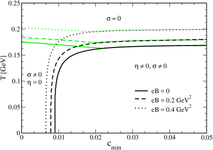
(a) Case Set I

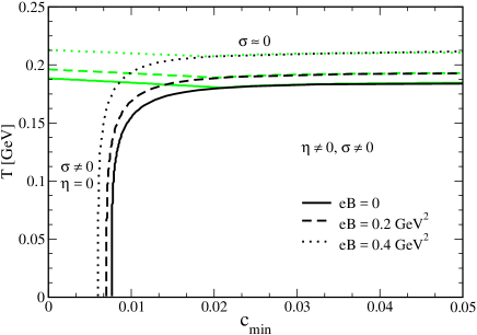
(b) Case Set II

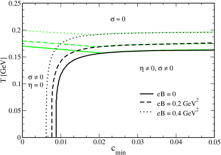
(c) Case Set III

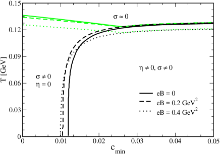
(d) Case with $G_{s}(eB,T)$

Figure 1: The $T-c_{\rm min}$ phase diagram, shown for three different values of external magnetic fields with the different parametrizations considered in this work. For these plots, we have considered the VEV of $a/f_{a}$ set as $\langle a\rangle/f_{a}=\pi$.

III Results and discussions

In this section we will present our results for the different quantities associated with the thermodynamics of the QCD axion in a hot and magnetized medium within the NJL model. Firstly, we will revisit the case with vanishing magnetic field Lu:2018ukl and discuss some relevant points related to these results. Next, we will move into the scenario with an external anisotropic magnetic field. Then, we will deal with the two different procedures, both related to the NJL model. First we will be working with a fixed coupling constant $G_{s}$, which accounts for only MC. Then, finally, we will also incorporate the IMC effect in our results using the effective $B$ and $T$ dependent coupling constant $G_{s}(eB,T)$ defined in the previous section, and discuss about the effects of both MC and IMC on the axionic QCD system.

III.1 The $eB=0$ case

The case of a vanishing magnetic field has recently been studied with a different parametrization in Ref. Lu:2018ukl . In the current study we will present some different aspects along with some of the quantities already evaluated in Ref. Lu:2018ukl , for the purposes of comparing between different parametrizations. This will be particularly useful as a way of quantifying the differences that different parametrizations can make on the results.

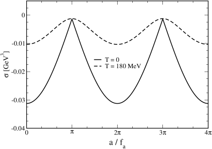
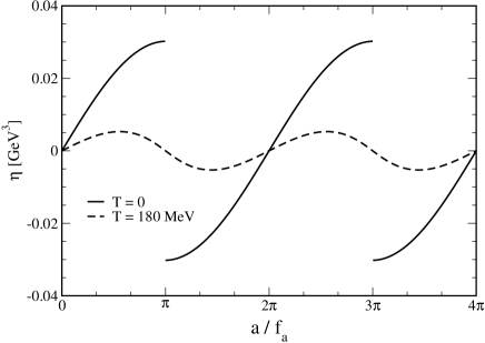
Figure 2: (a) Variation of $\sigma$ with respect to $a/f_{a}$ for two different values of $T$ and vanishing magnetic field. (b) Same variation done for $\eta$. The curves are obtained using the parameters from Set I shown in Table 1.

In Fig. 2 we have shown the variation of the physical condensates $\sigma$ and $\eta$ with the axion field $a$ scaled with $f_{a}$ for both $T=0$ and $T=180$ MeV. The sinusoidal behavior can be attributed to the $\sin(a/f_{a})$ and $\cos(a/f_{a})$ functions present in the effective mass $M$, appearing explicitly in the defined quantities in Eqs. (10)-(12). It is evident from Fig. 2 that the behaviors of $\sigma$ and $\eta$ differ whether the results are obtained for $T=0$ or for $T\neq 0$. As one can note from Fig. 2(b), at $T=0$ $\eta$ displays discontinuities for $a/f_{a}=(2j+1)\pi$, for $j=0,\,1,\,2,\ldots$, whereas for $a/f_{a}=2j\pi$ it vanishes. This result agrees with the Dashen’s phenomena Dashen:1970et , which predicts the existence of two degenerate vacua at $T=0$ and $a/f_{a}=(2j+1)\pi$ due to spontaneous $CP$ symmetry violation. Different signs of the two vacua indicates that they differ by a $CP$ transformation between them. But Dashen’s phenomena starts to break down with the increase in temperature. After a certain critical temperature $T_{c}$, the spontaneous $CP$ symmetry is restored and from the $CP$ violating phase ($\eta\neq 0,~{}\sigma\neq 0$), it returns to the phase of the ordinary chiral condensate ($\eta=0,~{}\sigma\neq 0$). This value of $T_{c}$ depends on the external magnetic field and parametrization. In fact, it can be realized from the phase diagram showed in Fig. 1 also, e.g., the solid curve in Fig. 1(a) confirms the fact that for $eB=0$ and using the parameters from the Set I case, the spontaneous $CP$ violating phase has already been disappeared before $T=180$ MeV. This is evident from Fig. 2(b), looking at the dashed curve at $T=180$ MeV, where now we have only one vacuum. On the other hand $\sigma$ attains its minimum value for $a/f_{a}=2j\pi$ and reaches the maximum value for $a/f_{a}=(2j+1)\pi$ for both $T=0$ and $T\neq 0$.

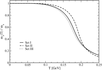
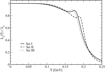
Figure 3: (a) Comparison between the variation of the axion mass ratio $m_{a}(T)/m_{a}$ with respect to $T$ for vanishing magnetic field with three different sets of parametrizations (see Table 1). (b) Same comparison done for the axion self-coupling ratio $\lambda_{a}(T)/\lambda_{a}$.

In Fig. 3 we have shown the comparison between three different sets of parametrizations listed in Table 1 for the variations of the temperature dependent axion mass $m_{a}(T)$ and the temperature dependent axion self-coupling $\lambda_{a}(T)$, scaled with their respective zero temperature values. One notices that after the value of $T\simeq 0.1$ GeV, the different parametrizations start to deviate from each other. For both the case of the axion mass and the axion self-coupling, a relatively rapid decrease is noticed around the chiral (pseudo critical) transition temperature $T_{c}$, while for the self-coupling a kink-like feature appears in this region.

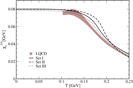
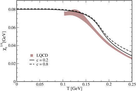
Figure 4: (a) Comparison between the variation of the topological susceptibility $\chi_{\rm{top}}$ with respect to $T$ and for vanishing magnetic field with three different parametrizations (see Table 1) along with the lattice QCD results from Borsanyi:2016ksw . (b) Comparison of $\chi_{\rm{top}}$ with respect to $T$ with two different values for the constant $c$, i.e., two different strengths of the axion interactions along with the lattice QCD results. In this case it is used the parameters from Set I shown in Table 1.

In Fig. 4 we show the results for the topological susceptibility $\chi_{\rm{top}}(T)$, for which we also have available the lattice QCD results Borsanyi:2016ksw at zero magnetic field. We have displayed the variation of $\chi_{\rm{top}}$ with respect to the temperature for the three different parametrizations sets previously mentioned and compared them both with the available lattice QCD results. As one can see from Fig. 4(a), the parameter sets I and III given in the Table 1 look more compatible with the lattice data. In this case, we can also see that $\chi_{\rm{top}}(T)$ has decreased substantially around $T_{c}$. This is a behavior matched by the corresponding lattice QCD data. In Fig. 4(b), we have plotted $\chi_{\rm{top}}(T)$ in the case of choosing two different values of the constant $c$, corresponding to two different strengths of the axion interaction. When the strength of the axion interaction is weaker, like in the case where $c=0.2$, the topological susceptibility is dragged down a little bit more at higher $T$ than in the higher strength case of $c=0.8$.

III.2 The case of finite magnetic field, $eB\neq 0$, but fixed coupling constant $G_{s}$

In this subsection we work with the same parametrization used for the $eB=0$ case, i.e., with a fixed coupling constant $G_{s}=5.022$ GeV^-2. As discussed earlier, with the fixed coupling constant we only consider the effects of magnetic catalysis in this case. Below we will also consider the more physical scenario, which accounts for the inverse magnetic catalysis effect that appears around the pseudo critical temperature.

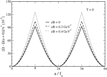
(a) Results for $T=0$.

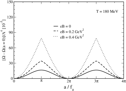
(b) Results for $T=180$ MeV.

Figure 5: Variation of the scaled axion contribution of the effective thermodynamic potential $\Omega-\Omega(a=0)$ with the scaled axion field $a/f_{a}$ for three different values of external magnetic field. The curves are obtained using the parameters from Set I shown in Table 1 for the magnetized medium and for two different values of temperature, i.e., for $T=0$ (a) and for $T=180$ MeV (b).

In Fig. 5, the variation of the scaled axionic part of the effective thermodynamic potential is shown with the scaled axion background field $a/f_{a}$ for three different values of the external magnetic field, namely, $eB=0,0.2$ GeV² and $0.4$ GeV², respectively. The aforementioned variation is shown for two different temperatures in the two panels shown in Fig. 5. It is apparent from these results that for both $T=0$ and $T=180$ MeV, with increasing magnetic field the value of the effective thermodynamic potential gets increased, which effectively also follows a valley-hill like structure. This behavior can be traced again due to the presence of the terms $\sin(a/f_{a})$ and $\cos(a/f_{a})$ in the effective mass $M$. It is also noticeable that with increasing temperature, the thermal effects start to melt down the amplitude of the axionic part of the thermodynamic potential, which is visible most prominently when we compare the case of $eB=0$ in Fig. 5 (a) and Fig. 5 (b) .

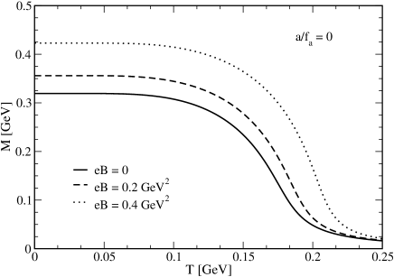
(a) Case for $a/f_{a}=0$.

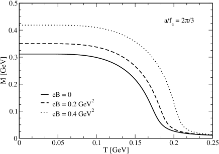
(b) Case for for $a/f_{a}=2\pi/3$.

Figure 6: Variation of the constituent quark mass $M$ with $T$ for three different values of the magnetic field. The plots are done with the parameters from Set I given in the Table 1 and for two different values of the scaled axion field, i.e., for $a/f_{a}=0$ and for $a/f_{a}=2\pi/3$.

In Fig. 6 we show the effects of the temperature and magnetic field on the effective dynamical mass $M(T,B)$, which in turn depends on the physical condensates $\sigma(T,B)$ and $\eta(T,B)$. The effect of MC is clearly evident from the results displayed in the figure: By increasing the magnetic field magnitude $eB$, the effective mass increases throughout the temperature range $T=0\,-\,250$ MeV. The effect of the axion field is also noticeable comparing the two plots in Fig. 6 as we see that the effective dynamical mass $M(T,B)$ gets slightly decreased with a finite value of the scaled axion field.

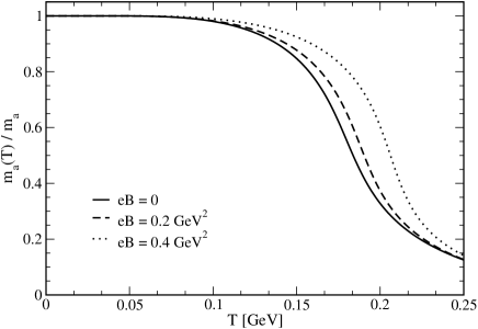
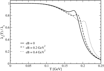
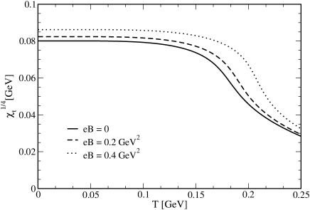
Figure 7: Panel (a): Variation of the axion mass ratio $m_{a}(T)/m_{a}$ with respect to $T$ for three different values for the external magnetic field. Panel (b): Same variation done for the axion self-coupling ratio $\lambda_{a}(T)/\lambda_{a}$. Panel (c): Likewise for the topological susceptibility $\chi_{\rm{top}}$. The plots are done with the parameters from Set I shown in the Table 1.

In Fig. 7 it is shown the temperature behavior for the axion mass and for the self-coupling, both scaled with their respective zero temperature values, for three different values for the external magnetic field. For both the cases shown in the figure, the magnetic catalysis effects are visible around the inflection point close to $T_{c}$. We can see the inflection points shifting towards higher values of $T$ for higher values of $eB$, a clear sign of MC. Similar behavior of MC is obtained in Fig. 7(c), where it is shown the topological susceptibility as a function of the temperature. The MC effect is visible throughout the temperature range. We can notice that the value of $\chi_{\rm{top}}^{1/4}$ at zero temperature goes up to $\sim 0.0865$ GeV for the highest value of $eB$ considered, $eB=0.4$ GeV${}^{2}\sim 20m_{\pi}^{2}$.

III.3 The case of considering a temperature and magnetic field dependent coupling $G_{s}(eB,T)$ constrained by lattice QCD

Finally, let us here explore the more physical scenario involving the effect of inverse magnetic catalysis around the transition temperature, originally predicted by lattice QCD for a hot and magnetized medium. As mentioned previously, for the purposes of incorporating IMC in the ambit of the NJL model, in this subsection we have used a temperature and magnetic field dependent coupling constant $G_{s}(eB,T)$.

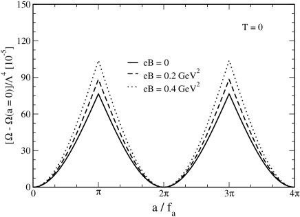
(a) Case for $T=0$.

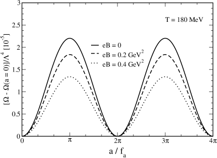
(b) Case for $T=180$ MeV.

Figure 8: Same as in Fig. 5, but considering now the effect of a $eB$ and $T$ dependent coupling constant $G_{s}(eB,T)$ for two different temperatures: Panel (a) $T=0$ and panel (b) $T=180$ MeV.

In Fig. 8 we have again plotted the scaled axion dependent part of the thermodynamic potential varying with respect to the scaled axion field. This time, using the fully temperature and magnetic field dependent coupling constant $G_{s}(eB,T)$, given by Eq. (30). The main qualitative and quantitative difference in this case with respect to that shown in the previous Fig. 5 can be noticed in Fig. 8, where the effect of IMC is evident throughout the whole range of the axion background field. For the case of $T=180$ MeV, i.e., $T\sim T_{c}$, we can see that with increasing magnetic field the amplitude of the thermodynamic potential gets decreased. For this case, the overall value of the scaled thermodynamic potential also becomes very low because of the low value of $G_{s}(eB,T)$ at higher temperatures. The strong dependence on the way the coupling constant is parametrized is evident comparing Fig. 5 with Fig. 8.

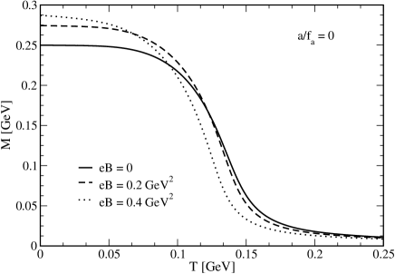
(a) Case for $a/f_{a}=0$.

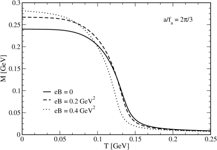
(b) Case for $a/f_{a}=2\pi/3$.

Figure 9: Same as shown in Fig. 6, but considering the $eB$ and $T$ dependent coupling constant $G_{s}(eB,T)$ for two different values of the scaled axion field, i.e. $a/f_{a}=0$ and $a/f_{a}=2\pi/3$.

In Fig. 9 we show the variation of the effective constituent quark mass $M$ with respect to $T$ and using the explicitly dependent on $B$ and $T$ coupling constant $G_{s}(eB,T)$. It clearly explores the full spectrum of hot magnetized medium showing both the MC and IMC effects for both vanishing and finite axion field. At zero to lower temperatures it shows the catalysis effect as higher $eB$ values correspond to higher effective mass. But at the higher temperatures, it goes through a crossover and around $T_{c}$ the behavior is completely opposite, emphasizing the occurrence of the inverse magnetic catalysis in that regime.

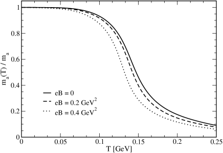
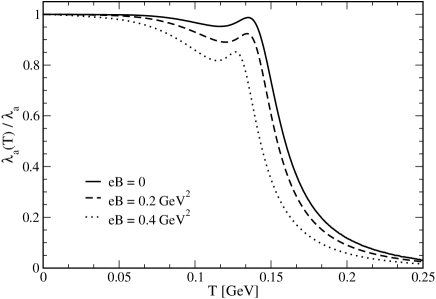
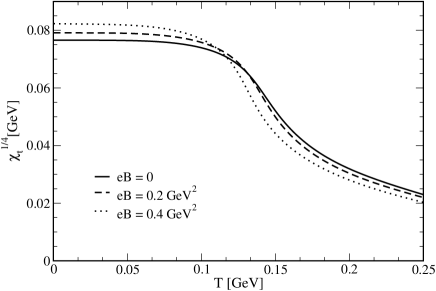
Figure 10: Same as in Fig. 7 but considering the fully $eB$ and $T$ dependent coupling constant $G_{s}(eB,T)$ for the axion mass ratio $m_{a}(T)/m_{a}$, panel (a), the axion self-coupling ratio $\lambda_{a}(T)/\lambda_{a}$, panel (b) and for the topological susceptibility, panel (c).

In Fig. 10 we have shown the variation of scaled axion mass, self-coupling and topological susceptibility with $T$ for the fully magnetic field and temperature dependent coupling constant $G_{s}(eB,T)$. The MC effect at lower temperature is not visible in Figs. 10(a) and 10(b) because of the scaling used, but for both these cases the IMC is clearly noticeable around $T_{c}$: The inflection points, indicating the pseudo critical temperature location, is shifted towards lower temperature with increasing magnetic fields. The kink-like feature in the position of the pseudo critical temperature location appearing in the axion self-coupling plot shows a similar behavior. In Fig. 10(c) the topological susceptibility is also shown in view of the fully $B$ and $T$ dependent coupling constant $G_{s}(eB,T)$, which again shows both the MC and the IMC effects in different temperature regimes with a crossover happening in between. The quantitative difference between the zero temperature values of $\chi_{\rm{top}}$ shown in Fig. 7(c) and Fig. 10(c) is solely due to the difference in the coupling constant $G_{s}$ parametrization, i.e., the difference between the extrapolation of lattice fitted $G_{s}(eB,T)\big{|}_{T,eB=0}=4.6311$ GeV^-2 with the fixed $G_{s}=5.022$ GeV^-2 case shown in Fig. 7(c).

Finally, as mentioned in Sec. II.4, at $T=0$ we can now predict the behavior of the magnetic field dependence of the topological susceptibility $\chi_{\rm{top}}$ using the magnetic field dependent coupling $G_{0}(eB)$. This is explicitly shown in Fig. 11, where the variation for both $G_{0}(eB)$ and when taking a fixed coupling constant, putting $B=0$ in Eq.(31), i.e., $G_{0}(eB=0)=4.50373$ GeV^-2, are considered.

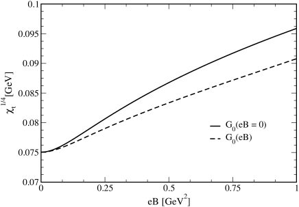
Figure 11: Variation of the topological susceptibility $\chi_{\rm{top}}$ with respect to $eB$ in the zero temperature case. The solid curve is for the $G_{0}(eB=0)$ and the dashed curve is when the fully magnetic field dependent coupling $G_{0}(eB)$ is considered.

(a) $\eta$ for $a/f_{a}=0$.

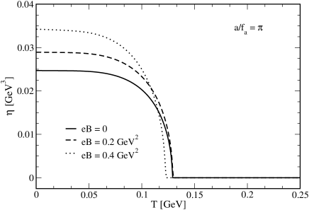
(b) $\eta$ for $a/f_{a}=\pi$.

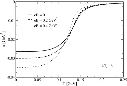
(c) $\sigma$ for $a/f_{a}=0$.

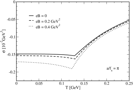
(d) $\sigma$ for $a/f_{a}=\pi$.

Figure 12: The temperature dependence for the condensates $\eta$ and $\sigma$ for three different values of external magnetic fields with $G_{s}(eB,T)$.

As a final remark here, we should point out that as a central theme of our present work, let us discuss about the effect of the spontaneous CP violation observed in our results. In Fig. 12, we have shown the variations for both the $\sigma$ and $\eta$ condensates with respect to the temperature and for three different values of the external magnetic field. As a consequence of our discussions and results up to this point, we have only considered the running coupling $G_{s}(eB,T)$ when getting these results. Also, for illustration purposes, we have chosen two specific values for $a/f_{a}$, i.e., $0$ and $\pi$, which we believe should suffice for our discussion. The result shown in Fig. 12(a) illustrates that there is no $CP$ violation happening at $a/f_{a}=0$, irrespective of the increasing temperature and external magnetic field. This result is compatible with the well known Vafa-Witten theorem Vafa:1984xg . Now, the results displayed in Fig. 12(b) clearly show the $CP$ violating $\eta\neq 0$ phase for $a/f_{a}=\pi$ in the lower temperature region. The external magnetic field dependence of the critical temperature $T_{c}(eB)$ is also quite visible from Fig. 12(b), which gradually decreases with increasing $eB$ (also in agreement with the IMC phenomena). This result helps to show both the spontaneous $CP$ symmetry breaking at $T=0$, i.e., Dashen’s phenomena, and the gradual restoration of the same at $T=T_{c}(eB)$. Then, in Figs. 12(c) and 12(d), they show similar variations for the chiral condensate. They mimic the nature of the constituent quark mass shown in Fig. 9(a). As a summary of the possible phases involved in our work, we can say that for $a/f_{a}=2j\pi$ we have only the chiral symmetry breaking phase, i.e., $\sigma\neq 0$ and $\eta=0$, which becomes restored at a temperature $T>0.2$ GeV, i.e., leading to $\sigma=\eta=0$. But for $a/f_{a}=(2j+1)\pi$, apart from the chiral phase transition (a crossover), we have another second order phase transition at a magnetic field dependent critical temperature $T_{c}(eB)$, when the spontaneous $CP$ violating phase gets restored. For $a/f_{a}=\pi$, these three phases have explicitly been shown in the $T-c_{\rm min}$ plane in Fig. 1.

IV Conclusion

In conclusion, we would like to convey that in the present work we have studied, for the first time as far as it is of our knowledge, the thermodynamics of QCD axions within the NJL model in a hot and magnetized medium by explicitly emphasizing the effects of two of the most appealing phenomena in this context, i.e., the magnetic catalysis and the inverse magnetic catalysis effects. In the process, we have studied the different behaviors shown by the condensates for two different values of the scaled axion field, i.e. $a/f_{a}=0$ and $\pi$, consistent with the well known Vafa-Witten theorem and Dashen’s phenomena respectively, leading to a discussion about the occurrence of different possible phases. Furthermore we have investigated the effect of the temperature and the external magnetic field explicitly on the measure of the spontaneous $CP$ violation, thereby showing the magnetic field dependence of the critical temperature for the spontaneous $CP$ symmetry restoration. Choosing the VEV of the axion field as a $CP$ violating term in the QCD action our results extend the previous results in the context of strong $CP$ violation Frank:2003ve ; Boomsma:2009eh ; Boomsma:2009yk ; Chatterjee:2014csa ; Fukushima:2001hr by incorporating Inverse Magnetic Catalysis effect in the medium using thermomagnetic field dependent coupling constant $G_{s}(eB,T)$. On top of that, the axion mass, self-coupling and topological susceptibility have their own significance regarding the study of cold dark matter, axion stars, the cooling anomaly problem in astrophysics, etc, and we have explored the effects of temperature and external magnetic field on these quantities. Finally throughout this present work, we have also explored the importance of evaluating the differences in the results when different parametrizations are considered in the context of an effective model for QCD. In this work, we have explicitly made this study in the context of the two-flavor NJL model applied to the QCD axion thermodynamics. These results thereby strengthen the claim of a strong dependence on parametrization within the NJL model.

V Acknowledgements

This work was partially supported by Conselho Nacional de Desenvolvimento Científico e Tecnológico (CNPq) under Grants No. 304758/2017-5 (R.L.S.F.), No. 136071/2018-0 (B.S.L.) and No. 302545/2017-4 (R.O.R.), Fundação Carlos Chagas Filho de Amparo à Pesquisa do Estado do Rio de Janeiro (FAPERJ) under Grant No. E-26/202.892/2017 (R.O.R.) and Coordenação de Aperfeiçoamento de Pessoal de Nível Superior (CAPES) (A.B.) - Brasil (CAPES)- Finance Code 001.

References

- (1) R. D. Peccei and H. R. Quinn, “CP Conservation in the Presence of Instantons,” Phys. Rev. Lett. 38, 1440 (1977). doi:10.1103/PhysRevLett.38.1440
- (2) S. Weinberg, “A New Light Boson?,” Phys. Rev. Lett. 40, 223 (1978). doi:10.1103/PhysRevLett.40.223
- (3) F. Wilczek, “Problem of Strong and Invariance in the Presence of Instantons,” Phys. Rev. Lett. 40, 279 (1978). doi:10.1103/PhysRevLett.40.279
- (4) D. J. E. Marsh, “Axion Cosmology,” Phys. Rept. 643, 1 (2016) doi:10.1016/j.physrep.2016.06.005 [arXiv:1510.07633 [astro-ph.CO]].
- (5) P. Sikivie and Q. Yang, “Bose-Einstein Condensation of Dark Matter Axions,” Phys. Rev. Lett. 103, 111301 (2009) doi:10.1103/PhysRevLett.103.111301 [arXiv:0901.1106 [hep-ph]].
- (6) P. H. Chavanis, “Phase transitions between dilute and dense axion stars,” Phys. Rev. D 98, no. 2, 023009 (2018) doi:10.1103/PhysRevD.98.023009 [arXiv:1710.06268 [gr-qc]].
- (7) P. Sikivie, “Experimental Tests of the Invisible Axion,” Phys. Rev. Lett. 51, 1415 (1983) Erratum: [Phys. Rev. Lett. 52, 695 (1984)]. doi:10.1103/PhysRevLett.51.1415, 10.1103/PhysRevLett.52.695.2
- (8) P. Sikivie, “Detection Rates for ’Invisible’ Axion Searches,” Phys. Rev. D 32, 2988 (1985) Erratum: [Phys. Rev. D 36, 974 (1987)]. doi:10.1103/PhysRevD.36.974, 10.1103/PhysRevD.32.2988
- (9) K. Van Bibber, N. R. Dagdeviren, S. E. Koonin, A. Kerman and H. N. Nelson, “Proposed experiment to produce and detect light pseudoscalars,” Phys. Rev. Lett. 59, 759 (1987). doi:10.1103/PhysRevLett.59.759
- (10) S. De Panfilis et al., “Limits on the Abundance and Coupling of Cosmic Axions at 4.5-Microev m(a) 5.0-Microev,” Phys. Rev. Lett. 59, 839 (1987). doi:10.1103/PhysRevLett.59.839
- (11) C. Hagmann, P. Sikivie, N. S. Sullivan and D. B. Tanner, “Results from a search for cosmic axions,” Phys. Rev. D 42, 1297 (1990). doi:10.1103/PhysRevD.42.1297
- (12) P. Sikivie, D. B. Tanner and Y. Wang, “Axion detection in the milli-eV mass range,” Phys. Rev. D 50, 4744 (1994) doi:10.1103/PhysRevD.50.4744
- (13) G. G. Raffelt, “Astrophysical axion bounds,” Lect. Notes Phys. 741, 51 (2008) doi:10.1007/978-3-540-73518-23 [hep-ph/0611350].
- (14) M. Giannotti, I. Irastorza, J. Redondo and A. Ringwald, “Cool WISPs for stellar cooling excesses,” JCAP 1605, no. 05, 057 (2016) doi:10.1088/1475-7516/2016/05/057 [arXiv:1512.08108 [astro-ph.HE]].
- (15) J. Keller and A. Sedrakian,“Axions from cooling compact stars”, Nucl. Phys. A897, 62 (2013). doi:10.1016/j.nuclphysa.2012.11.004
- (16) A. Sedrakian, “Axion cooling of neutron stars”, Phys. Rev. D 93, 065044 (2016). doi:10.1103/PhysRevD.93.065044.
- (17) A. Sedrakian, “Axion cooling of neutron stars. II. Beyond hadronic axions”, Phys. Rev. D 99, 043011 (2019). doi:10.1103/PhysRevD.99.043011.
- (18) A. Arvanitaki and S. Dubovsky, “Exploring the String Axiverse with Precision Black Hole Physics,” Phys. Rev. D 83 (2011) 044026 doi:10.1103/PhysRevD.83.044026 [arXiv:1004.3558 [hep-th]].
- (19) A. Arvanitaki, M. Baryakhtar and X. Huang, “Discovering the QCD Axion with Black Holes and Gravitational Waves,” Phys. Rev. D 91, no. 8, 084011 (2015) doi:10.1103/PhysRevD.91.084011 [arXiv:1411.2263 [hep-ph]].
- (20) P. Brun et al. [MADMAX Collaboration], “A new experimental approach to probe QCD axion dark matter in the mass range above 40 eV,” Eur. Phys. J. C 79, no. 3, 186 (2019) doi:10.1140/epjc/s10052-019-6683-x [arXiv:1901.07401 [physics.ins-det]].
- (21) M. S. Turner, “Cosmic and Local Mass Density of Invisible Axions,” Phys. Rev. D 33, 889 (1986). doi:10.1103/PhysRevD.33.889
- (22) S. P. Klevansky, “The Nambu-Jona-Lasinio model of quantum chromodynamics,” Rev. Mod. Phys. 64, 649 (1992). doi:10.1103/RevModPhys.64.649
- (23) G. Landini and E. Meggiolaro, “Study of the interactions of the axion with mesons and photons using a chiral effective Lagrangian model,” arXiv:1906.03104 [hep-ph].
- (24) M. Frank, M. Buballa and M. Oertel, “Flavor mixing effects on the QCD phase diagram at nonvanishing isospin chemical potential: One or two phase transitions?,” Phys. Lett. B 562, 221 (2003) doi:10.1016/S0370-2693(03)00607-5 [hep-ph/0303109].
- (25) J. K. Boomsma and D. Boer, “The High temperature CP-restoring phase transition at theta = pi,” Phys. Rev. D 80, 034019 (2009) doi:10.1103/PhysRevD.80.034019 [arXiv:0905.4660 [hep-ph]].
- (26) J. K. Boomsma and D. Boer, “The Influence of strong magnetic fields and instantons on the phase structure of the two-flavor NJL model,” Phys. Rev. D 81, 074005 (2010) doi:10.1103/PhysRevD.81.074005 [arXiv:0911.2164 [hep-ph]].
- (27) B. Chatterjee, H. Mishra and A. Mishra, “ violation and chiral symmetry breaking in hot and dense quark matter in the presence of a magnetic field,” Phys. Rev. D 91, no. 3, 034031 (2015) doi:10.1103/PhysRevD.91.034031 [arXiv:1409.3454 [hep-ph]].
- (28) K. Fukushima, K. Ohnishi and K. Ohta, “Topological susceptibility at zero and finite temperature in the Nambu-Jona-Lasinio model,” Phys. Rev. C 63, 045203 (2001) doi:10.1103/PhysRevC.63.045203 [nucl-th/0101062].
- (29) G. ’t Hooft, “Computation of the Quantum Effects Due to a Four-Dimensional Pseudoparticle,” Phys. Rev. D 14, 3432 (1976) Erratum: [Phys. Rev. D 18, 2199 (1978)]. doi:10.1103/PhysRevD.18.2199.3, 10.1103/PhysRevD.14.3432
- (30) G. ’t Hooft, “How Instantons Solve the U(1) Problem,” Phys. Rept. 142, 357 (1986). doi:10.1016/0370-1573(86)90117-1
- (31) V. P. Gusynin, V. A. Miransky and I. A. Shovkovy, “Dimensional reduction and catalysis of dynamical symmetry breaking by a magnetic field,” Nucl. Phys. B 462, 249 (1996) doi:10.1016/0550-3213(96)00021-1 [hep-ph/9509320].
- (32) G. S. Bali, F. Bruckmann, G. Endrödi, Z. Fodor, S. D. Katz, S. Krieg, A. Schafer and K. K. Szabo, “The QCD phase diagram for external magnetic fields,” JHEP 1202, 044 (2012) doi:10.1007/JHEP02(2012)044 [arXiv:1111.4956 [hep-lat]].
- (33) G. S. Bali, F. Bruckmann, G. Endrödi, Z. Fodor, S. D. Katz and A. Schafer, “QCD quark condensate in external magnetic fields,” Phys. Rev. D 86, 071502 (2012) doi:10.1103/PhysRevD.86.071502 [arXiv:1206.4205 [hep-lat]].
- (34) E. S. Fraga and A. J. Mizher, “Chiral symmetry restoration and strong CP violation in a strong magnetic background,” PoS CPOD 2009, 037 (2009) doi:10.22323/1.071.0037 [arXiv:0910.4525 [hep-ph]].
- (35) A. J. Mizher and E. S. Fraga, “CP violation and chiral symmetry restoration in the hot linear sigma model in a strong magnetic background,” Nucl. Phys. A 831, 91 (2009) doi:10.1016/j.nuclphysa.2009.09.004 [arXiv:0810.5162 [hep-ph]].
- (36) A. J. Mizher and E. S. Fraga, “CP Violation in the Linear Sigma Model,” Nucl. Phys. A 820, 247C (2009) doi:10.1016/j.nuclphysa.2009.01.061 [arXiv:0810.4115 [hep-ph]].
- (37) E. S. Fraga and A. J. Mizher, “Can a strong magnetic background modify the nature of the chiral transition in QCD?,” Nucl. Phys. A 820, 103C (2009) doi:10.1016/j.nuclphysa.2009.01.026 [arXiv:0810.3693 [hep-ph]].
- (38) K. Kawarabayashi and N. Ohta, “On the Partial Conservation of the U(1) Current,” Prog. Theor. Phys. 66, 1789 (1981). doi:10.1143/PTP.66.1789
- (39) V. Baluni, “CP Violating Effects in QCD,” Phys. Rev. D 19, 2227 (1979). doi:10.1103/PhysRevD.19.2227
- (40) R. J. Crewther, P. Di Vecchia, G. Veneziano and E. Witten, “Chiral Estimate of the Electric Dipole Moment of the Neutron in Quantum Chromodynamics,” Phys. Lett. 88B, 123 (1979) Erratum: [Phys. Lett. 91B, 487 (1980)]. doi:10.1016/0370-2693(80)91025-4, 10.1016/0370-2693(79)90128-X
- (41) C. A. Baker et al., “An Improved experimental limit on the electric dipole moment of the neutron,” Phys. Rev. Lett. 97, 131801 (2006) doi:10.1103/PhysRevLett.97.131801 [hep-ex/0602020].
- (42) J. M. Pendlebury et al., “Revised experimental upper limit on the electric dipole moment of the neutron,” Phys. Rev. D 92, no. 9, 092003 (2015) doi:10.1103/PhysRevD.92.092003 [arXiv:1509.04411 [hep-ex]].
- (43) F.-K. Guo et al., “The electric dipole moment of the neutron from 2+1 flavor lattice QCD,” Phys. Rev. Lett. 115, no. 6, 062001 (2015) doi:10.1103/PhysRevLett.115.062001 [arXiv:1502.02295 [hep-lat]].
- (44) T. Bhattacharya, V. Cirigliano, R. Gupta, H. W. Lin and B. Yoon, “Neutron Electric Dipole Moment and Tensor Charges from Lattice QCD,” Phys. Rev. Lett. 115, no. 21, 212002 (2015) doi:10.1103/PhysRevLett.115.212002 [arXiv:1506.04196 [hep-lat]].
- (45) M. Buballa, “NJL model analysis of quark matter at large density,” Phys. Rept. 407, 205 (2005) doi:10.1016/j.physrep.2004.11.004 [hep-ph/0402234].
- (46) Z. Y. Lu and M. Ruggieri, “Effect of the chiral phase transition on axion mass and self-coupling,” arXiv:1811.05102 [hep-ph].
- (47) G. Grilli di Cortona, E. Hardy, J. Pardo Vega and G. Villadoro, “The QCD axion, precisely,” JHEP 1601, 034 (2016) doi:10.1007/JHEP01(2016)034 [arXiv:1511.02867 [hep-ph]].
- (48) D. Ebert, K. G. Klimenko, M. A. Vdovichenko and A. S. Vshivtsev, “Magnetic oscillations in dense cold quark matter with four fermion interactions,” Phys. Rev. D 61, 025005 (2000) doi:10.1103/PhysRevD.61.025005 [hep-ph/9905253].
- (49) M. A. Vdovichenko, A. S. Vshivtsev and K. G. Klimenko, “Magnetic catalysis and magnetic oscillations in the Nambu-Jona-Lasinio model,” Phys. Atom. Nucl. 63, 470 (2000) [Yad. Fiz. 63, 542 (2000)]. doi:10.1134/1.855661
- (50) D. Ebert and K. G. Klimenko, “Quark droplets stability induced by external magnetic field,” Nucl. Phys. A 728, 203 (2003) doi:10.1016/j.nuclphysa.2003.08.021 [hep-ph/0305149].
- (51) D. P. Menezes, M. Benghi Pinto, S. S. Avancini, A. Perez Martinez and C. Providência, “Quark matter under strong magnetic fields in the Nambu-Jona-Lasinio Model,” Phys. Rev. C 79, 035807 (2009) doi:10.1103/PhysRevC.79.035807 [arXiv:0811.3361 [nucl-th]].
- (52) D. P. Menezes, M. Benghi Pinto, S. S. Avancini and C. Providência, “Quark matter under strong magnetic fields in the su(3) Nambu-Jona-Lasinio Model,” Phys. Rev. C 80, 065805 (2009) doi:10.1103/PhysRevC.80.065805 [arXiv:0907.2607 [nucl-th]].
- (53) R. L. S. Farias, K. P. Gomes, G. I. Krein and M. B. Pinto, “Importance of asymptotic freedom for the pseudocritical temperature in magnetized quark matter,” Phys. Rev. C 90, no. 2, 025203 (2014) doi:10.1103/PhysRevC.90.025203 [arXiv:1404.3931 [hep-ph]].
- (54) P. G. Allen, A. G. Grunfeld and N. N. Scoccola, “Magnetized color superconducting cold quark matter within the SU(2)f NJL model: A novel regularization scheme,” Phys. Rev. D 92, no. 7, 074041 (2015) doi:10.1103/PhysRevD.92.074041 [arXiv:1508.04724 [hep-ph]].
- (55) D. C. Duarte, R. L. S. Farias, P. H. A. Manso and R. O. Ramos, “Relativistic BEC-BCS Crossover in a magnetized Nambu-Jona-Lasinio Model,” J. Phys. Conf. Ser. 706, no. 5, 052010 (2016). doi:10.1088/1742-6596/706/5/052010
- (56) S. S. Avancini, W. R. Tavares and M. B. Pinto, “Properties of magnetized neutral mesons within a full RPA evaluation,” Phys. Rev. D 93, no. 1, 014010 (2016) doi:10.1103/PhysRevD.93.014010 [arXiv:1511.06261 [hep-ph]].
- (57) D. C. Duarte, P. G. Allen, R. L. S. Farias, P. H. A. Manso, R. O. Ramos and N. N. Scoccola, “BEC-BCS crossover in a cold and magnetized two color NJL model,” Phys. Rev. D 93, no. 2, 025017 (2016) doi:10.1103/PhysRevD.93.025017 [arXiv:1510.02756 [hep-ph]].
- (58) S. S. Avancini, R. L. S. Farias, M. Benghi Pinto, W. R. Tavares and V. S. Timóteo, “ pole mass calculation in a strong magnetic field and lattice constraints,” Phys. Lett. B 767, 247 (2017) doi:10.1016/j.physletb.2017.02.002 [arXiv:1606.05754 [hep-ph]].
- (59) R. L. S. Farias, V. S. Timóteo, S. S. Avancini, M. B. Pinto and G. Krein, “Thermo-magnetic effects in quark matter: Nambu–Jona-Lasinio model constrained by lattice QCD,” Eur. Phys. J. A 53, no. 5, 101 (2017) doi:10.1140/epja/i2017-12320-8 [arXiv:1603.03847 [hep-ph]].
- (60) M. Coppola, P. Allen, A. G. Grunfeld and N. N. Scoccola, “Magnetized color superconducting quark matter under compact star conditions: Phase structure within the SU(2)f NJL model,” Phys. Rev. D 96, no. 5, 056013 (2017) doi:10.1103/PhysRevD.96.056013 [arXiv:1707.03795 [hep-ph]].
- (61) S. S. Avancini, V. Dexheimer, R. L. S. Farias and V. S. Timóteo, “Anisotropy in the equation of state of strongly magnetized quark matter within the Nambu–Jona-Lasinio model,” Phys. Rev. C 97, no. 3, 035207 (2018) doi:10.1103/PhysRevC.97.035207 [arXiv:1709.02774 [hep-ph]].
- (62) S.S. Avancini, R.L.S. Farias, N.N. Scoccola and W. R. Tavares, “NJL-type models in the presence of intense magnetic fields: the role of the regularization prescription”, Phys. Rev. D 99,116002 (2019). doi:10.1103/PhysRevD.99.116002
- (63) S.S. Avancini, R.L.S. Farias and W. R. Tavares, “Neutral meson properties in hot and magnetized quark matter: A new magnetic field independent regularization scheme applied to an NJL-type model”, Phys. Rev. D 99, 056009 (2019). doi:10.1103/PhysRevD.99.056009
- (64) S. Schramm, B. Muller and A. J. Schramm, “Quark - anti-quark condensates in strong magnetic fields,” Mod. Phys. Lett. A 7, 973 (1992). doi:10.1142/S0217732392000860.
- (65) B. Chatterjee, H. Mishra and A. Mishra, “Vacuum structure and chiral symmetry breaking in strong magnetic fields for hot and dense quark matter,” Phys. Rev. D 84, 014016 (2011) doi:10.1103/PhysRevD.84.014016 [arXiv:1101.0498 [hep-ph]].
- (66) G. N. Ferrari, A. F. Garcia and M. B. Pinto, “Chiral Transition Within Effective Quark Models Under Magnetic Fields,” Phys. Rev. D 86, 096005 (2012) doi:10.1103/PhysRevD.86.096005 [arXiv:1207.3714 [hep-ph]].
- (67) M. Ferreira, P. Costa, D. P. Menezes, C. Providência and N. Scoccola, “Deconfinement and chiral restoration within the SU(3) Polyakov–Nambu–Jona-Lasinio and entangled Polyakov–Nambu–Jona-Lasinio models in an external magnetic field,” Phys. Rev. D 89, no. 1, 016002 (2014) Addendum: [Phys. Rev. D 89, no. 1, 019902 (2014)] doi:10.1103/PhysRevD.89.016002, 10.1103/PhysRevD.89.019902 [arXiv:1305.4751 [hep-ph]].
- (68) F. Bruckmann, G. Endrödi and T. G. Kovacs, “Inverse magnetic catalysis and the Polyakov loop,” JHEP 1304, 112 (2013) doi:10.1007/JHEP04(2013)112 [arXiv:1303.3972 [hep-lat]].
- (69) G. Endrödi, “Critical point in the QCD phase diagram for extremely strong background magnetic fields,” JHEP 1507, 173 (2015) doi:10.1007/JHEP07(2015)173 [arXiv:1504.08280 [hep-lat]].
- (70) L. Yu, J. Van Doorsselaere and M. Huang, “Inverse Magnetic Catalysis in the three-flavor NJL model with axial-vector interaction,” Phys. Rev. D 91, no. 7, 074011 (2015) doi:10.1103/PhysRevD.91.074011 [arXiv:1411.7552 [hep-ph]].
- (71) S. Mao, “Inverse magnetic catalysis in Nambu???Jona-Lasinio model beyond mean field,” Phys. Lett. B 758, 195 (2016) doi:10.1016/j.physletb.2016.05.018 [arXiv:1602.06503 [hep-ph]].
- (72) A. Ayala, M. Loewe, A. J. Mizher and R. Zamora, “Inverse magnetic catalysis for the chiral transition induced by thermo-magnetic effects on the coupling constant,” Phys. Rev. D 90, no. 3, 036001 (2014) doi:10.1103/PhysRevD.90.036001 [arXiv:1406.3885 [hep-ph]].
- (73) A. Ayala, M. Loewe and R. Zamora, “Inverse magnetic catalysis in the linear sigma model with quarks,” Phys. Rev. D 91, no. 1, 016002 (2015) doi:10.1103/PhysRevD.91.016002 [arXiv:1406.7408 [hep-ph]].
- (74) C. Providência, M. Ferreira and P. Costa, “Inverse magnetic catalysis in the Polyakov-Nambu-Jona-Lasinio and entangled Polyakov-Nambu-Jona-Lasinio models,” Acta Phys. Polon. Supp. 8, no. 1, 207 (2015) doi:10.5506/APhysPolBSupp.8.207 [arXiv:1412.8308 [hep-ph]].
- (75) M. Ferreira, P. Costa, O. Lourenço, T. Frederico and C. Providência, “Inverse magnetic catalysis in the (2+1)-flavor Nambu-Jona-Lasinio and Polyakov-Nambu-Jona-Lasinio models,” Phys. Rev. D 89, no. 11, 116011 (2014) doi:10.1103/PhysRevD.89.116011 [arXiv:1404.5577 [hep-ph]].
- (76) E. J. Ferrer, V. de la Incera and X. J. Wen, “Quark Antiscreening at Strong Magnetic Field and Inverse Magnetic Catalysis,” Phys. Rev. D 91, no. 5, 054006 (2015) doi:10.1103/PhysRevD.91.054006 [arXiv:1407.3503 [nucl-th]].
- (77) G. Endrödi and G. Markó. “Magnetized baryons and the QCD phase diagram: NJL model meets the lattice”.[arXiv:1905.02103 [hep-lat]]
- (78) R. F. Dashen, Phys. Rev. D 3, 1879 (1971). doi:10.1103/PhysRevD.3.1879
- (79) C. Vafa and E. Witten, Phys. Rev. Lett. 53, 535 (1984). doi:10.1103/PhysRevLett.53.535
- (80) S. Borsanyi et al., “Calculation of the axion mass based on high-temperature lattice quantum chromodynamics,” Nature 539, no. 7627, 69 (2016) doi:10.1038/nature20115 [arXiv:1606.07494 [hep-lat]].