Trade-offs in Large-Scale Distributed Tuplewise Estimation and Learning

Abstract

The development of cluster computing frameworks has allowed practitioners to scale out various statistical estimation and machine learning algorithms with minimal programming effort. This is especially true for machine learning problems whose objective function is nicely separable across individual data points, such as classification and regression. In contrast, statistical learning tasks involving pairs (or more generally tuples) of data points — such as metric learning, clustering or ranking — do not lend themselves as easily to data-parallelism and in-memory computing. In this paper, we investigate how to balance between statistical performance and computational efficiency in such distributed tuplewise statistical problems. We first propose a simple strategy based on occasionally repartitioning data across workers between parallel computation stages, where the number of repartitioning steps rules the trade-off between accuracy and runtime. We then present some theoretical results highlighting the benefits brought by the proposed method in terms of variance reduction, and extend our results to design distributed stochastic gradient descent algorithms for tuplewise empirical risk minimization. Our results are supported by numerical experiments in pairwise statistical estimation and learning on synthetic and real-world datasets.

Keywords: Distributed Machine Learning $\cdot$ Distributed Data Processing $\cdot$ $U$-Statistics $\cdot$ Stochastic Gradient Descent $\cdot$ AUC Optimization

1 Introduction

Statistical machine learning has seen dramatic development over the last decades. The availability of massive datasets combined with the increasing need to perform predictive/inference/optimization tasks in a wide variety of domains has given a considerable boost to the field and led to successful applications. In parallel, there has been an ongoing technological progress in the architecture of data repositories and distributed systems, allowing to process ever larger (and possibly complex, high-dimensional) data sets gathered on distributed storage platforms. This trend is illustrated by the development of many easy-to-use cluster computing frameworks for large-scale distributed data processing. These frameworks implement the data-parallel setting, in which data points are partitioned across different machines which operate on their partition in parallel. Some striking examples are Apache Spark [26] and Petuum [25], the latter being fully targeted to machine learning. The goal of such frameworks is to abstract away the network and communication aspects in order to ease the deployment of distributed algorithms on large computing clusters and on the cloud, at the cost of some restrictions in the types of operations and parallelism that can be efficiently achieved. However, these limitations as well as those arising from network latencies or the nature of certain memory-intensive operations are often ignored or incorporated in a stylized manner in the mathematical description and analysis of statistical learning algorithms (see e.g., [2, 15, 4, 1]). The implementation of statistical methods proved to be theoretically sound may thus be hardly feasible in a practical distributed system, and seemingly minor adjustments to scale-up these procedures can turn out to be disastrous in terms of statistical performance, see e.g. the discussion in [19]. This greatly restricts their practical interest in some applications and urges the statistics and machine learning communities to get involved with distributed computation more deeply [3].

In this paper, we propose to study these issues in the context of tuplewise estimation and learning problems, where the statistical quantities of interest are not basic sample means but come in the form of averages over all pairs (or more generally, $d$-tuples) of data points. Such data functionals are known as $U$-statistics [20, 16], and many empirical quantities describing global properties of a probability distribution fall in this category (e.g., the sample variance, the Gini mean difference, Kendall’s tau coefficient). $U$-statistics are also natural empirical risk measures in several learning problems such as ranking [13], metric learning [24], cluster analysis [11] and risk assessment [5]. The behavior of these statistics is well-understood and a sound theory for empirical risk minimization based on $U$-statistics is now documented in the machine learning literature [13], but the computation of a $U$-statistic poses a serious scalability challenge as it involves a summation over an exploding number of pairs (or $d$-tuples) as the dataset grows in size. In the centralized (single machine) setting, this can be addressed by appropriate subsampling methods, which have been shown to achieve a nearly optimal balance between computational cost and statistical accuracy [12]. Unfortunately, naive implementations in the case of a massive distributed dataset either greatly damage the accuracy or are inefficient due to a lot of network communication (or disk I/O). This is due to the fact that, unlike basic sample means, a $U$-statistic is not separable across the data partitions.

Our main contribution is to design and analyze distributed methods for statistical estimation and learning with $U$-statistics that guarantee a good trade-off between accuracy and scalability. Our approach incorporates an occasional data repartitioning step between parallel computing stages in order to circumvent the limitations induced by data partitioning over the cluster nodes. The number of repartitioning steps allows to trade-off between statistical accuracy and computational efficiency. To shed light on this phenomenon, we first study the setting of statistical estimation, precisely quantifying the variance of estimates corresponding to several strategies. Thanks to the use of Hoeffding’s decomposition [18], our analysis reveals the role played by each component of the variance in the effect of repartitioning. We then discuss the extension of these results to statistical learning and design efficient and scalable stochastic gradient descent algorithms for distributed empirical risk minimization. Finally, we carry out some numerical experiments on pairwise estimation and learning tasks on synthetic and real-world datasets to support our results from an empirical perspective.

The paper is structured as follows. Section 2 reviews background on $U$-statistics and their use in statistical estimation and learning, and discuss the common practices in distributed data processing. Section 3 deals with statistical tuplewise estimation: we introduce our general approach for the distributed setting and derive (non-)asymptotic results describing its accuracy. Section 4 extends our approach to statistical tuplewise learning. We provide experiments supporting our results in Section 5, and we conclude in Section 6. Proofs, technical details and additional results can be found in the supplementary material.

2 Background

In this section, we first review the definition and properties of $U$-statistics, and discuss some popular applications in statistical estimation and learning. We then discuss the recent randomized methods designed to scale up tuplewise statistical inference to large datasets stored on a single machine. Finally, we describe the main features of cluster computing frameworks.

2.1 $U$-Statistics: Definition and Applications

$U$-statistics are the natural generalization of i.i.d. sample means to tuples of points. We state the definition of $U$-statistics in their generalized form, where points can come from $K\geq 1$ independent samples. Note that we recover classic sample mean statistics in the case where $K=d_{1}=1$.

Definition 1

(Generalized $U$-statistic) Let $K\geq 1$ and $(d_{1},\;\ldots,\;d_{K})\in\mathbb{N}^{*K}$. For each $k\in\{1,\dots,K\}$, let $\mathbf{X}_{\{1,\;\ldots,\;n_{k}\}}=(X^{(k)}_{1},\;\ldots,\;X^{(k)}_{n_{k}})$ be an independent sample of size $n_{k}\geq d_{k}$ composed of i.i.d. random variables with values in some measurable space ${\cal X}_{k}$ with distribution $F_{k}(dx)$. Let $h:{\cal X}_{1}^{d_{1}}\times\cdots\times{\cal X}_{K}^{d_{K}}\rightarrow\mathbb{R}$ be a measurable function, square integrable with respect to the probability distribution $\mu=F_{1}^{\otimes d_{1}}\otimes\cdots\otimes F_{K}^{\otimes d_{K}}$. Assume w.l.o.g. that $h(\mathbf{x}^{(1)},\;\ldots,\;\mathbf{x}^{(K)})$ is symmetric within each block of arguments $\mathbf{x}^{(k)}$ (valued in ${\cal X}^{d_{k}}_{k}$). The generalized (or $K$-sample) $U$-statistic of degrees $(d_{1},\;\ldots,\;d_{K})$ with kernel $H$ is defined as

$$U_{\mathbf{n}}(h)=\frac{1}{\prod_{k=1}^{K}\binom{n_{k}}{d_{k}}}\sum_{I_{1}}\ldots\sum_{I_{K}}h(\mathbf{X}^{(1)}_{I_{1}},\;\mathbf{X}^{(2)}_{I_{2}},\;\ldots,\;\mathbf{X}^{(K)}_{I_{K}}),$$ (1)

where $\sum_{I_{k}}$ denotes the sum over all $\binom{n_{k}}{d_{k}}$ subsets $\mathbf{X}^{(k)}_{I_{k}}=(X^{(k)}_{i_{1}},\;\ldots,\;X^{(k)}_{i_{d_{k}}})$ related to a set $I_{k}$ of $d_{k}$ indexes $1\leq i_{1}<\ldots<i_{d_{k}}\leq n_{k}$ and $\mathbf{n}=(n_{1},\;\ldots,\;n_{K})$.

The $U$-statistic $U_{\mathbf{n}}(h)$ is known to have minimum variance among all unbiased estimators of the parameter $\mu(h)=\mathbb{E}\big{[}h(X^{(1)}_{1},\;\ldots,\;X^{(1)}_{d_{1}},\;\ldots,\;X^{(K)}_{1},\;\ldots,\;X^{(K)}_{d_{K}})\big{]}$. The price to pay for this low variance is a complex dependence structure exhibited by the terms involved in the average (1), as each data point appears in multiple tuples. The (non)asymptotic behavior of $U$-statistics and $U$-processes (i.e., collections of $U$-statistics indexed by classes of kernels) can be investigated by means of linearization techniques [18] combined with decoupling methods [16], reducing somehow their analysis to that of basic i.i.d. averages or empirical processes. One may refer to [20] for an account of the asymptotic theory of $U$-statistics, and to [23] (Chapter 12 therein) and [16] for nonasymptotic results.

$U$-statistics are commonly used as point estimators for inferring certain global properties of a probability distribution as well as in statistical hypothesis testing. Popular examples include the (debiased) sample variance, obtained by setting $K=1$, $d_{1}=2$ and $h(x_{1},x_{2})=(x_{1}-x_{2})^{2}$, the Gini mean difference, where $K=1$, $d_{1}=2$ and $h(x_{1},x_{2})=|x_{1}-x_{2}|$, and Kendall’s tau rank correlation, where $K=2$, $d_{1}=d_{2}=1$ and $h((x_{1},y_{1}),(x_{2},y_{1}))=\mathbb{I}\{(x_{1}-x_{2})\cdot(y_{1}-y_{2})>0\}$.

$U$-statistics also correspond to empirical risk measures in statistical learning problems such as clustering [11], metric learning [24] and multipartite ranking [14]. The generalization ability of minimizers of such criteria over a class $\mathcal{H}$ of kernels can be derived from probabilistic upper bounds for the maximal deviation of collections of centered $U$-statistics under appropriate complexity conditions on $\mathcal{H}$ (e.g., finite VC dimension) [13, 12]. Below, we describe the example of multipartite ranking used in our numerical experiments (Section 5). We refer to [12] for details on more learning problems involving $U$-statistics.

Example 1 (Multipartite Ranking)

Consider items described by a random vector of features $X\in\mathcal{X}$ with associated ordinal labels $Y\in\{1,\ldots,K\}$, where $K\geq 2$. The goal of multipartite ranking is to learn to rank items in the same preorder as that defined by the labels, based on a training set of labeled examples. Rankings are generally defined through a scoring function $s:\mathcal{X}\rightarrow\mathbb{R}$ transporting the natural order on the real line onto $\mathcal{X}$. Given $K$ independent samples, the empirical ranking performance of $s(x)$ is evaluated by means of the empirical ${\rm VUS}$ (Volume Under the $\rm ROC$ Surface) criterion [14]:

$$\widehat{VUS}(s)=\frac{1}{\prod^{K}_{k=1}n_{k}}\sum^{n_{1}}_{i_{1}=1}\ldots\sum^{n_{K}}_{i_{K}=1}{\mathbb{I}}\{s(X^{(1)}_{i_{1}})<\ldots<s(X^{(K)}_{i_{K}})\},$$ (2)

which is a $K$-sample $U$-statistic of degree $(1,\ldots,1)$ with kernel $h_{s}(x_{1},\;\ldots,\;x_{K})=\mathbb{I}\{s(x_{1})<\ldots<s(x_{K})\}$.

2.2 Large-Scale Tuplewise Inference with Incomplete $U$-statistics

The cost related to the computation of the $U$-statistic (1) rapidly explodes as the sizes of the samples increase. Precisely, the number of terms involved in the summation is $\binom{n_{1}}{d_{1}}\times\cdots\times\binom{n_{K}}{d_{K}}$, which is of order $O(n^{d_{1}+\ldots+d_{K}})$ when the $n_{k}$’s are all asymptotically equivalent. Whereas computing $U$-statistics based on subsamples of smaller size would severely increase the variance of the estimation, the notion of incomplete generalized $U$-statistic [6] enables to significantly mitigate this computational problem while maintaining a good level of accuracy.

Definition 2

(Incomplete generalized $U$-statistic) Let $B\geq 1$. The incomplete version of the $U$-statistic (1) based on $B$ terms is defined by:

$$\widetilde{U}_{B}(H)=\frac{1}{B}\sum_{I=(I_{1},\;\ldots,\,I_{K})\in\mathcal{D}_{B}}h(\mathbf{X}^{(1)}_{I_{1}},\;\ldots,\;\mathbf{X}^{(K)}_{I_{K}})$$ (3)

where $\mathcal{D}_{B}$ is a set of cardinality $B$ built by sampling uniformly with replacement in the set $\Lambda$ of vectors of tuples $((i^{(1)}_{1},\;\ldots,\;i^{(1)}_{d_{1}}),\;\ldots,\;(i^{(K)}_{1},\;\ldots,\;i^{(K)}_{d_{K}}))$, where $1\leq i^{(k)}_{1}<\ldots<i^{(k)}_{d_{k}}\leq n_{k}$ and $1\leq k\leq K$.

Note incidentally that the subsets of indices can be selected by means of other sampling schemes [12], but sampling with replacement is often preferred due to its simplicity. In practice, the parameter $B$ should be picked much smaller than the total number of tuples to reduce the computational cost. Like (1), the quantity (3) is an unbiased estimator of $\mu(H)$ but its variance is naturally larger:

$$\mathrm{Var}(\widetilde{U}_{B}(h))=\Big{(}1-\frac{1}{B}\Big{)}\mathrm{Var}(U_{\mathbf{n}}(h))+\frac{1}{B}\mathrm{Var}(h(X^{(1)}_{1},\;\ldots,\;X^{(K)}_{d_{K}})).$$ (4)

The recent work in [12] has shown that the maximal deviations between $\eqref{eq:UstatG}$ and (3) over a class of kernels $\mathcal{H}$ of controlled complexity decrease at a rate of order $O(1/\sqrt{B})$ as $B$ increases. An important consequence of this result is that sampling $B=O(n)$ terms is sufficient to preserve the learning rate of order $O_{\mathbb{P}}(\sqrt{\log n/n})$ of the minimizer of the complete risk (1), whose computation requires to average $O(n^{d_{1}+\ldots+d_{K}})$ terms. In contrast, the distribution of a complete $U$-statistic built from subsamples of reduced sizes $n^{\prime}_{k}$ drawn uniformly at random is quite different from that of an incomplete $U$-statistic based on $B=\prod_{k=1}^{K}\binom{n^{\prime}_{k}}{d_{k}}$ terms sampled with replacement in $\Lambda$, although they involve the summation of the same number of terms. Empirical minimizers of such a complete $U$-statistic based on subsamples achieve a much slower learning rate of $O_{\mathbb{P}}(\sqrt{\log(n)/n^{1/(d_{1}+\ldots+d_{K})}})$. We refer to [12] for details and additional results.

We have seen that approximating complete $U$-statistics by incomplete ones is a theoretically and practically sound approach to tackle large-scale tuplewise estimation and learning problems. However, as we shall see later, the implementation is far from straightforward when data is stored and processed in standard distributed computing frameworks, whose key features are recalled below.

2.3 Practices in Distributed Data Processing

Data-parallelism, i.e. partitioning the data across different machines which operate in parallel, is a natural approach to store and efficiently process massive datasets. This strategy is especially appealing when the key stages of the computation to be executed can be run in parallel on each partition of the data. As a matter of fact, many estimation and learning problems can be reduced to (a sequence of) local computations on each machine followed by a simple aggregation step. This is the case of gradient descent-based algorithms applied to standard empirical risk minimization problems, as the objective function is nicely separable across individual data points. Optimization algorithms operating in the data-parallel setting have indeed been largely investigated in the machine learning community, see [3, 8, 1, 22] and references therein for some recent work.

Because of the prevalence of data-parallel applications in large-scale machine learning, data analytics and other fields, the past few years have seen a sustained development of distributed data processing frameworks designed to facilitate the implementation and the deployment on computing clusters. Besides the seminal MapReduce framework [17], which is not suitable for iterative computations on the same data, one can mention Apache Spark [26], Apache Flink [10] and the machine learning-oriented Petuum [25]. In these frameworks, the data is typically first read from a distributed file system (such as HDFS, Hadoop Distributed File System) and partitioned across the memory of each machine in the form of an appropriate distributed data structure. The user can then easily specify a sequence of distributed computations to be performed on this data structure (map, filter, reduce, etc.) through a simple API which hides low-level distributed primitives (such as message passing between machines). Importantly, these frameworks natively implement fault-tolerance (allowing efficient recovery from node failures) in a way that is also completely transparent to the user.

While such distributed data processing frameworks come with a lot of benefits for the user, they also restrict the type of computations that can be performed efficiently on the data. In the rest of this paper, we investigate these limitations in the context of tuplewise estimation and learning problems, and propose solutions to achieve a good trade-off between accuracy and scalability.

3 Distributed Tuplewise Statistical Estimation

In this section, we focus on the problem of tuplewise statistical estimation in the distributed setting (an extension to statistical learning is presented in Section 4). We consider a set of $N\geq 1$ workers in a complete network graph (i.e., any pair of workers can exchange messages). For convenience, we assume the presence of a master node, which can be one of the workers and whose role is to aggregate estimates computed by all workers.

For ease of presentation, we restrict our attention to the case of two sample $U$-statistics of degree $(1,1)$ ($K=2$ and $d_{1}=d_{2}=1$), see Remark 1 in Section 3.3 for extensions to the general case. We denote by $\mathcal{D}_{n}=\left\{X_{1},\ldots,X_{n}\right\}$ the first sample and by $\mathcal{Q}_{m}=\left\{Z_{1},\ldots,Z_{m}\right\}$ the second sample (of sizes $n$ and $m$ respectively). These samples are distributed across the $N$ workers. For $i\in\{1,\dots,N\}$, we denote by $\mathcal{R}_{i}$ the subset of data points held by worker $i$ and, unless otherwise noted, we assume for simplicity that all subsets are of equal size $|\mathcal{R}_{i}|=\frac{n+m}{N}\in\mathbb{N}$. The notations $\mathcal{R}_{i}^{X}$ and $\mathcal{R}_{i}^{Z}$ respectively denote the subset of data points held by worker $i$ from $\mathcal{D}_{n}$ and $\mathcal{Q}_{m}$, with $\mathcal{R}_{i}^{X}\cup\mathcal{R}_{i}^{Z}=\mathcal{R}_{i}$. We denote their (possibly random) cardinality by $n_{i}=|\mathcal{R}_{i}^{X}|$ and $m_{i}=|\mathcal{R}_{i}^{Z}|$. Given a kernel $h$, the goal is to compute a good estimate of the parameter $U(h)=\mathbb{E}[h(X_{1},Z_{1})]$ while meeting some computational and communication constraints.

3.1 Naive Strategies

Before presenting our approach, we start by introducing two simple (but ineffective) strategies to compute an estimate of $U(h)$. The first one is to compute the complete two-sample $U$-statistic associated with the full samples $\mathcal{D}_{n}$ and $\mathcal{Q}_{m}$:

$$U_{\mathbf{n}}(h)=\frac{1}{nm}\sum_{k=1}^{n}\sum_{l=1}^{m}h(X_{k},Z_{l}),$$ (5)

with $\mathbf{n}=(n,m)$. While $U_{\mathbf{n}}(h)$ has the lowest variance among all unbiased estimates that can be computed from $(\mathcal{D}_{n},\mathcal{Q}_{m})$, computing it is a highly undesirable solution in the distributed setting where each worker only has access to a subset of the dataset. Indeed, ensuring that each possible pair is seen by at least one worker would require massive data communication over the network. Note that a similar limitation holds for incomplete versions of (5) as defined in Definition 2.

A feasible strategy to go around this problem is for each worker to compute the complete $U$-statistic associated with its local subsample $\mathcal{R}_{i}$, and to send it to the master node who averages all contributions. This leads to the estimate

$$U_{\mathbf{n},N}(h)=\frac{1}{N}\sum_{i=1}^{N}U_{\mathcal{R}_{i}}(h)\quad\text{where }U_{\mathcal{R}_{i}}(h)=\frac{1}{n_{i}m_{i}}\sum_{k\in\mathcal{R}_{i}^{X}}\sum_{l\in\mathcal{R}_{i}^{Z}}h(X_{k},Z_{l}).$$ (6)

Note that if $\min(n_{i},m_{i})=0$, we simply set $U_{\mathcal{R}_{i}}(h)=0$.

Alternatively, as the $\mathcal{R}_{i}$’s may be large, each worker can compute an incomplete $U$-statistic $\widetilde{U}_{B,\mathcal{R}_{i}}(h)$ with $B$ terms instead of $U_{\mathcal{R}_{i}}$, leading to the estimate

$$\widetilde{U}_{\mathbf{n},N,B}(h)=\frac{1}{N}\sum_{i=1}^{N}\widetilde{U}_{B,\mathcal{R}_{i}}(h)\quad\text{where }\widetilde{U}_{B,\mathcal{R}_{i}}(h)=\frac{1}{B}\sum_{(k,l)\in\mathcal{R}_{i,B}}h(X_{k},Z_{l}),$$ (7)

with $\mathcal{R}_{i,B}$ a set of $B$ pairs built by sampling uniformly with replacement from the local subsample $\mathcal{R}_{i}^{X}\times\mathcal{R}_{i}^{Z}$.

As shown in Section 3.3, strategies (6) and (7) have the undesirable property that their accuracy decreases as the number of workers $N$ increases. This motivates our proposed approach, introduced in the following section.

3.2 Proposed Approach

The naive strategies presented above are either accurate but very expensive (requiring a lot of communication across the network), or scalable but potentially inaccurate. The approach we promote here is of disarming simplicity and aims at finding a sweet spot between these two extremes. The idea is based on repartitioning the dataset a few times across workers (we keep the repartitioning scheme abstract for now and postpone the discussion of concrete choices to subsequent sections). By alternating between parallel computation and repartitioning steps, one considers several estimates based on the same data points. This allows to observe a greater diversity of pairs and thereby refine the quality of our final estimate, at the cost of some additional communication.

Formally, let $T$ be the number of repartitioning steps. We denote by $\mathcal{R}_{i}^{t}$ the subsample of worker $i$ after the $t$-th repartitioning step, and by $U_{\mathcal{R}_{i}^{t}}(h)$ the complete $U$-statistic associated with $\mathcal{R}_{i}^{t}$. At each step $t\in\{1,\dots,T\}$, each worker $i$ computes $U_{\mathcal{R}_{i}^{t}}(h)$ and sends it to the master node. After $T$ steps, the master node has access to the following estimate:

$$\widehat{U}_{\mathbf{n},N,T}(h)=\frac{1}{T}\sum_{t=1}^{T}U_{\mathbf{n},N}^{t}(h),$$ (8)

where $U_{\mathbf{n},N}^{t}(h)=\frac{1}{N}\sum_{i=1}^{N}U_{\mathcal{R}_{i}^{t}}(h)$. Similarly as before, workers may alternatively compute incomplete $U$-statistics $\widetilde{U}_{B,\mathcal{R}_{i}^{t}}(h)$ with $B$ terms. The estimate is then:

$$\widetilde{U}_{\mathbf{n},N,B,T}(h)=\frac{1}{T}\sum_{t=1}^{T}\widetilde{U}_{\mathbf{n},N,B}^{t}(h),$$ (9)

where $\widetilde{U}_{\mathbf{n},N,B}^{t}(h)=\frac{1}{N}\sum_{i=1}^{N}\widetilde{U}_{B,\mathcal{R}_{i}^{t}}(h)$. These statistics, and those introduced in Section 3.1 which do not rely on repartition, are summarized in Figure 1.

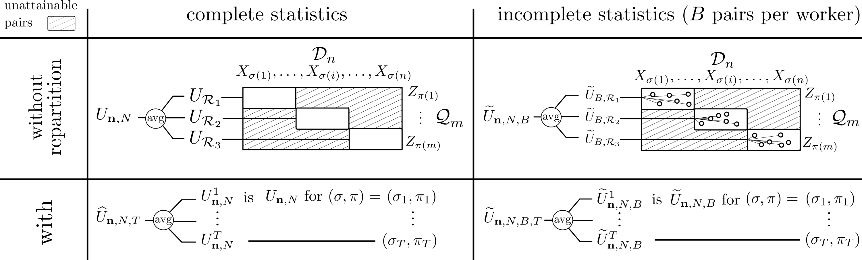
Figure 1: Graphical summary of the statistics that we compare: with/without repartition and with/without subsampling. Note that $\{(\sigma_{t},\pi_{t})\}_{t=1}^{T}$ denotes a set of $T$ independent couples of random permutations in $\mathfrak{S}_{n}\times\mathfrak{S}_{m}$.

Of course, the repartitioning operation is rather costly in terms of runtime so $T$ should be kept to a reasonably small value. We illustrate this trade-off by the analysis presented in the next section.

3.3 Analysis

In this section, we analyze the statistical properties of the various estimators introduced above. We focus here on repartitioning by proportional sampling without replacement (prop-SWOR). Prop-SWOR creates partitions that contain the same proportion of elements of each sample: specifically, it ensures that at any step $t$ and for any worker $i$, $|\mathcal{R}^{t}_{i}|=\frac{n+m}{N}$ with $|\mathcal{R}_{i}^{t,X}|=\frac{n}{N}$ and $|\mathcal{R}_{i}^{t,Z}|=\frac{m}{N}$. We discuss the practical implementation of this repartitioning scheme as well as some alternative choices in Section 3.4.

All estimators are unbiased when repartitioning is done with prop-SWOR. We will thus compare their variance. Our main technical tool is a linearization technique for $U$-statistics known as Hoeffding’s Decomposition (see [18, 13, 12]).

Definition 3

(Hoeffding’s decomposition) Let $h_{1}(x)=\mathbb{E}[h(x,Z_{1})]$, $h_{2}(z)=\mathbb{E}[h(X_{1},z)]$ and $h_{0}(x,z)=h(x,z)-h_{1}(x)-h_{2}(z)+U(h)$. $U_{\mathbf{n}}(h)-U(h)$ can be written as a sum of three orthogonal terms:

$$U_{\mathbf{n}}(h)-U(h)=T_{n}(h)+T_{m}(h)+W_{\mathbf{n}}(h),$$

where $T_{n}(h)=\frac{1}{n}\sum_{k=1}^{n}h_{1}(X_{k})-U(h)$ and $T_{m}(h)=\frac{1}{m}\sum_{l=1}^{n}h_{2}(Z_{l})-U(h)$ are sums of independent r.v, while $W_{\mathbf{n}}(h)=\frac{1}{nm}\sum_{k=1}^{n}\sum_{l=1}^{m}h_{0}(X_{k},Z_{l})$ is a degenerate $U$-statistic (i.e., $\mathbb{E}[h(X_{1},Z_{1})|X_{1}]=U(h)$ and $\mathbb{E}[h(X_{1},Z_{1})|Z_{1}]=U(h)$).

This decomposition is very convenient as the two terms $T_{n}(h)$ and $T_{m}(h)$ are decorrelated and the analysis of $W_{\mathbf{n}}(h)$ (a degenerate $U$-statistic) is well documented [18, 13, 12]. It will allow us to decompose the variance of the estimators of interest into single-sample components $\sigma_{1}^{2}=\text{Var}(h_{1}(X))$ and $\sigma_{2}^{2}=\text{Var}(h_{2}(Z))$ on the one hand, and a pairwise component $\sigma_{0}^{2}=\text{Var}(h_{0}(X_{1},Z_{1}))$ on the other hand. Denoting $\sigma^{2}=\text{Var}(h(X_{1},Z_{1}))$, we have $\sigma^{2}=\sigma_{0}^{2}+\sigma_{1}^{2}+\sigma_{2}^{2}$.

It is well-known that the variance of the complete $U$-statistic $U_{\mathbf{n}}(h)$ can be written as $\text{Var}(U_{\mathbf{n}}(h))=\frac{\sigma_{1}^{2}}{n}+\frac{\sigma_{2}^{2}}{m}+\frac{\sigma_{0}^{2}}{nm}$ (see supplementary material for details). Our first result gives the variance of the estimators which do not rely on a repartitioning of the data with respect to the variance of $U_{\mathbf{n}}(h)$.

Theorem 1

If the data is distributed over workers using prop-SWOR, we have:

$$\text{Var}(U_{\mathbf{n},N}(h)) =\text{Var}(U_{\mathbf{n}}(h))+(N-1)\frac{\sigma_{0}^{2}}{nm},$$

$$\text{Var}(\widetilde{U}_{\mathbf{n},N,B}(h)) =\left(1-\frac{1}{B}\right)\text{Var}(U_{\mathbf{n},N}(h))+\frac{\sigma^{2}}{NB}.$$

Theorem 1 precisely quantifies the excess variance due to the distributed setting if one does not use repartitioning. Two important observations are in order. First, the variance increase is proportional to the number of workers $N$, which clearly defeats the purpose of distributed processing. Second, this increase only depends on the pairwise component $\sigma_{0}^{2}$ of the variance. In other words, the average of $U$-statistics computed independently over the local partitions contains all the information useful to estimate the single-sample contributions, but fails to accurately estimate the pairwise contributions. The resulting estimates thus lead to significantly larger variance when the choice of kernel and the data distributions imply that $\sigma_{0}^{2}$ is large compared to $\sigma_{2}^{1}$ and/or $\sigma_{1}^{2}$. The extreme case happens when $U_{\textbf{n}}(h)$ is a degenerate $U$-statistic, i.e. $\sigma_{1}^{2}=\sigma_{2}^{2}=0$ and $\sigma_{0}^{2}>0$, which is verified for example when $h(x,z)=x\cdot z$ and $X,Z$ are both centered random variables.

We now characterize the variance of the estimators that leverage data repartitioning steps.

Theorem 2

If the data is distributed and repartitioned between workers using prop-SWOR, we have:

$$\text{Var}(\widehat{U}_{\mathbf{n},N,T}(h)) =\text{Var}(U_{\mathbf{n}}(h))+(N-1)\frac{\sigma_{0}^{2}}{nmT},$$

$$\text{Var}(\widetilde{U}_{\mathbf{n},N,B,T}(h)) =\text{Var}(\widehat{U}_{\mathbf{n},N,T}(h))-\frac{1}{TB}\text{Var}(U_{\mathbf{n},N}(h))+\frac{\sigma^{2}}{NTB}.$$

Theorem 2 shows that the value of repartitioning arises from the fact that the term accounting for the pairwise variance in $\widehat{U}_{\textbf{n},N,T}(h)$ is $T$ times lower than that of $U_{\mathbf{n},N}(h)$. This validates the fact that repartitioning is beneficial when the pairwise variance term is significant in front of the other terms. Interestingly, Theorem 2 also implies that for a fixed budget of evaluated pairs, using all pairs on each worker is always a dominant strategy over using incomplete approximations. Specifically, we can show that under the constraint $NBT=nmT_{0}/N$, $\text{Var}(\widehat{U}_{\mathbf{n},N,T_{0}}(h))$ is always smaller than $\text{Var}(\widetilde{U}_{\mathbf{n},N,B,T}(h))$, see supplementary material for details. Note that computing complete $U$-statistics also require fewer repartitioning steps to evaluate the same number of pairs (i.e., $T_{0}\leq T$).

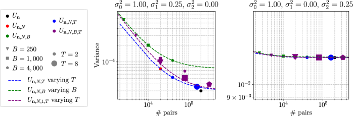
Figure 2: Theoretical variance as a function of the number of evaluated pairs for different estimators under prop-SWOR, with $n=100,000$, $m=200$ and $N=100$.

We conclude the analysis with a visual illustration of the variance of various estimators with respect to the number of pairs they evaluate. We consider the imbalanced setting where $n\gg m$, which is commonly encountered in applications such as imbalanced classification, bipartite ranking and anomaly detection. In this case, it suffices that $\sigma_{2}^{2}$ be small for the influence of the pairwise component of the variance to be significant, see Fig. 2 (left). The figure also confirms that complete estimators dominate their incomplete counterparts. On the other hand, when $\sigma_{2}^{2}$ is not small, the variance of $U_{\textbf{n}}$ mostly originates from the rarity of the minority sample, hence repartitioning does not provide estimates that are significantly more accurate (see Fig. 2, right). We refer to Section 5 for experiments on concrete tasks with synthetic and real data.

Remark 1 (Extension to high-order $U$-statistics)

The extension of our analysis to general $U$-statistics is straightforward and left to the reader (see [12] for a review of the relevant technical tools). We stress the fact that the benefits of repartitioning are even stronger for higher-order $U$-statistics ($K>2$ and/or larger degrees) because higher-order components of the variance are also affected.

3.4 Practical Considerations and Other Repartitioning Schemes

The analysis above assumes that repartitioning is done using prop-SWOR, which has the advantage of exactly preserving the proportion of points from the two samples $\mathcal{D}_{n}$ and $\mathcal{Q}_{m}$ even in the event of significant imbalance in their size. However, a naive implementation of prop-SWOR requires some coordination between workers at each repartitioning step. To avoid exchanging many messages, we propose that the workers agree at the beginning of the protocol on a numbering of the workers, a numbering of the points in each sample, and a random seed to use in a pseudorandom number generator. This allows the workers to implement prop-SWOR without any further coordination: at each repartitioning step, they independently draw the same two random permutations over $\{1,\dots,n\}$ and $\{1,\dots,m\}$ using the common random seed and use these permutations to assign each point to a single worker.

Of course, other repartitioning schemes can be used instead of prop-SWOR. A natural choice is sampling without replacement (SWOR), which does not require any coordination between workers. However, the partition sizes generated by SWOR are random. This is a concern in the case of imbalanced samples, where the probability that a worker $i$ does not get any point from the minority sample (and thus no pair to compute a local estimate) is non-negligible. For these reasons, it is difficult to obtain exact and concise theoretical variances for the SWOR case, but we show in the supplementary material that the results with SWOR should not deviate too much from those obtained with prop-SWOR. For completeness, in the supplementary material we also analyze the case of proportional sampling with replacement (prop-SWR): results are quantitatively similar, aside from the fact that redistribution also corrects for the loss of information that occurs because of sampling with replacement.

Finally, we note that deterministic repartitioning schemes may be used in practice for simplicity. For instance, the repartition method in Apache Spark relies on a deterministic shuffle which preserves the size of the partitions.

4 Extensions to Stochastic Gradient Descent for ERM

The results of Section 3 can be extended to statistical learning in the empirical risk minimization framework. In such problems, given a class of kernels $\mathcal{H}$, one seeks the minimizer of (6) or (8) depending on whether repartition is used. Under appropriate complexity assumptions on $\mathcal{H}$ (e.g., of finite VC dimension), excess risk bounds for such minimizers can be obtained by combining our variance analysis of Section 3 with the control of maximal deviations based on Bernstein-type concentration inequalities as done in [13, 12]. Due to the lack of space, we leave the details of such analysis to the readers and focus on the more practical scenario where the ERM problem is solved by gradient-based optimization algorithms.

4.1 Gradient-based Empirical Minimization of $U$-statistics

In the setting of interest, the class of kernels to optimize over is indexed by a real-valued parameter $\theta\in\mathbb{R}^{q}$ representing the model. Adapting the notations of Section 3, the kernel $h:{\cal X}_{1}\times{\cal X}_{2}\times\mathbb{R}^{q}\rightarrow\mathbb{R}$ then measures the performance of a model $\theta\in\mathbb{R}^{q}$ on a given pair, and is assumed to be convex and smooth in $\theta$. Empirical Risk Minimization (ERM) aims at finding $\theta\in\mathbb{R}^{q}$ minimizing

$$U_{\mathbf{n}}(\theta)=\frac{1}{nm}\sum_{k=1}^{n}\sum_{l=1}^{m}h(X_{k},Z_{l};\theta).$$ (10)

The minimizer can be found by means of Gradient Descent (GD) techniques. Starting at iteration $s=1$ from an initial model $\theta_{1}\in\mathbb{R}^{q}$ and given a learning rate $\gamma>0$, GD consists in iterating over the following update:

$$\theta_{s+1}=\theta_{s}-\gamma\nabla_{\theta}U_{\mathbf{n}}(\theta_{s}).$$ (11)

Note that the gradient $\nabla_{\theta}U_{\mathbf{n}}(\theta)$ is itself a $U$-statistic with kernel given by $\nabla_{\theta}H$, and its computation is very expensive in the large-scale setting. In this regime, Stochastic Gradient Descent (SGD) is a natural alternative to GD which is known to provide a better trade-off between the amount of computation and the performance of the resulting model [7]. Following the discussion of Section 2.2, a natural idea to implement SGD is to replace the gradient $\nabla_{\theta}U_{\mathbf{n}}(\theta)$ in (11) by an unbiased estimate given by an incomplete $U$-statistic. The work of [21] shows that SGD converges much faster than if the gradient is estimated using a complete $U$-statistic based on subsamples with the same number of terms.

However, as in the case of estimation, the use of standard complete or incomplete $U$-statistics turns out to be impractical in the distributed setting. Building upon the arguments of Section 3, we propose a more suitable strategy.

4.2 Repartitioning for Stochastic Gradient Descent

The approach we propose is to alternate between SGD steps using within-partition pairs and repartitioning the data across workers. We introduce a parameter $n_{r}\in\mathbb{Z}^{+}$ corresponding to the number of iterations of SGD between each redistribution of the data. For notational convenience, we let $r(s):=\lceil s/n_{r}\rceil$ so that for any worker $i$, $\mathcal{R}^{r(s)}_{i}$ denotes its data partition at iteration $s\geq 1$ of SGD.

Given a local batch size $B$, at each iteration $s$ of SGD, we propose to adapt the strategy (9) by having each worker $i$ compute a local gradient estimate using a set $\mathcal{R}^{s}_{i,B}$ of $B$ randomly sampled pairs in its current local partition $\mathcal{R}^{r(s)}_{i}$:

$$\nabla_{\theta}\widetilde{U}_{B,\mathcal{R}^{r(s)}_{i}}(\theta_{s})=\frac{1}{B}\sum_{(k,l)\in\mathcal{R}^{s}_{i,B}}\nabla_{\theta}h(X_{k},Z_{l};\theta_{s}).$$

This local estimate is then sent to the master node who averages all contributions, leading to the following global gradient estimate:

$$\nabla_{\theta}\widetilde{U}_{\mathbf{n},N,B}(\theta_{s})=\frac{1}{N}\sum_{i=1}^{N}\nabla_{\theta}\widetilde{U}_{B,\mathcal{R}^{r(s)}_{i}}(\theta_{s}).$$ (12)

The master node then takes a gradient descent step as in (11) and broadcasts the updated model $\theta_{s+1}$ to the workers.

Following our analysis in Section 3, repartitioning the data allows to reduce the variance of the gradient estimates, which is known to greatly impact the convergence rate of SGD (see e.g. [9], Theorem 6.3 therein). When $n_{r}=+\infty$, data is never repartitioned and the algorithm minimizes an average of local $U$-statistics, leading to suboptimal performance. On the other hand, $n_{r}=1$ corresponds to repartitioning at each iteration of SGD, which minimizes the variance but is very costly and makes SGD pointless. We expect the sweet spot to lie between these two extremes: the dominance of $\widehat{U}_{\mathbf{n},N,T}$ over $\widetilde{U}_{\mathbf{n},N,B,T}$ established in Section 3.3, combined with the common use of small batch size $B$ in SGD, suggests that occasional redistributions are sufficient to correct for the loss of information incurred by the partitioning of data. We illustrate these trade-offs experimentally in the next section.

5 Numerical Results

In this section, we illustrate the importance of repartitioning for estimating and optimizing the Area Under the ROC Curve (AUC) through a series of numerical experiments. The corresponding $U$-statistic is the two-sample version of the multipartite ranking VUS introduced in Example 1 (Section 2.1). The first experiment focuses on the estimation setting considered in Section 3. The second experiment shows that redistributing the data across workers, as proposed in Section  4, allows for more efficient mini-batch SGD. All experiments use prop-SWOR and are conducted in a simulated environment.

Estimation experiment.

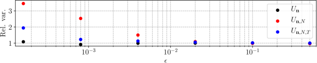
Figure 3: Relative variance estimated over $5000$ runs, $n=5000$, $m=50$, $N=10$ and $T=4$. Results are divided by the true variance of $U_{\mathbf{n}}$ deduced from (13) and Theorem 1.

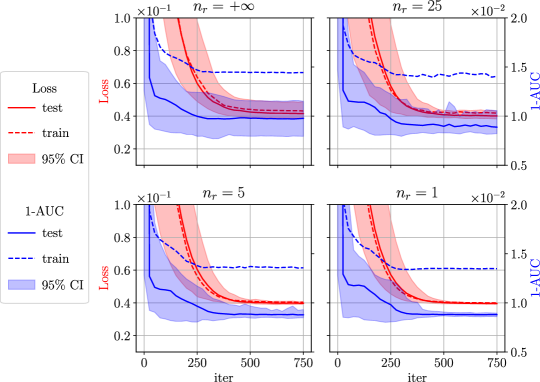
Figure 4: Learning dynamics for different repartition frequencies computed over 100 runs.

We seek to illustrate the importance of redistribution for estimating two-sample $U$-statistics with the concrete example of the AUC. The AUC is obtained by choosing the kernel $h(x,z)={\mathbb{I}}\{z<x\}$, and is widely used as a performance measure in bipartite ranking and binary classification with class imbalance. Recall that our results of Section 3.3 highlighted the key role of the pairwise component of the variance $\sigma_{0}^{2}$ being large compared to the single-sample components. In the case of the AUC, this happens when the data distributions are such that the expected outcome using single-sample information is far from the truth, e.g. in the presence of hard pairs. We illustrate this on simple discrete distributions for which we can compute $\sigma_{0}^{2}$, $\sigma_{1}^{2}$ and $\sigma_{2}^{2}$ in closed form. Consider positive points $X\in\{0,2\}$, negative points $Z\in\{-1,+1\}$ and $\mathbb{P}\left(X=2\right)=q$, $\mathbb{P}\left(Z=+1\right)=p$. It follows that:

$$\sigma_{1}^{2} =p^{2}q(1-q),\quad\sigma_{2}^{2}=(1-q)^{2}p(1-p),\text{ and }\sigma^{2}=p(1-p+pq)(1-q).$$ (13)

Assume that the scoring function has a small probability $\epsilon$ to assign a low score to a positive instance or a large score to a negative instance. In our formal setting, this translates into letting $p=1-q=\epsilon$ for a small $\epsilon>0$, which implies that $\frac{\sigma_{0}^{2}}{\sigma_{1}^{2}+\sigma_{2}^{2}}=\frac{1-\epsilon}{2\epsilon}\underset{\epsilon\to 0}{\to}\infty$. We thus expect that as the true AUC $U(h)=1-\epsilon^{2}$ gets closer to $1$, repartitioning the dataset becomes more critical to achieve good relative precision. This is confirmed numerically, as shown in Fig. 3. Note that in practice, settings where the AUC is very close to $1$ are very common as they correspond to well-functioning systems, such as face recognition systems.

Learning experiment.

We now turn to AUC optimization, which is the task of learning a scoring function $s:\mathcal{X}\rightarrow\mathbb{R}$ that optimizes the VUS criterion (2) with $K=2$ in order to discriminate between a negative and a positive class. We learn a linear scoring function $s_{w,b}(x)=w^{\top}x+b$, and optimize a continuous and convex surrogate of (2) based on the hinge loss. The resulting loss function to minimize is a two-sample U-statistic with kernel $g_{w,b}(x,z)=\max(0,1+s_{w,b}(x)-s_{w,b}(z))$ indexed by the parameters $(w,b)$ of the scoring function, to which we add a small L2 regularization term of $0.05\left\lVert w\right\rVert_{2}^{2}$.

We use the shuttle dataset, a classic dataset for anomaly detection. It contains roughly 49,000 points in dimension 9, among which only 7% (approx. 3,500) are anomalies. A high accuracy is expected for this dataset. To monitor the generalization performance, we keep 20% of the data as our test set, corresponding to 700 points of the minority class and approx. 9,000 points of the majority class. The test performance is measured with complete statistics over the 6.3 million pairs. The training set consists of the remaining data points, which we distribute over $N=100$ workers. This leads to approx. $10,200$ pairs per worker. The gradient estimates are calculated following (12) with batch size $B=100$. We use an initial learning rate of $0.01$ with a momentum of $0.9$. As there are more than 100 million possible pairs in the training dataset, we monitor the training loss and accuracy on a fixed subset of $4.5\times 10^{5}$ randomly sampled pairs.

Fig. 4 shows the evolution of the continuous loss and the true AUC on the training and test sets along the iteration for different values of $n_{r}$, from $n_{r}=1$ (repartition at each iteration) to $n_{r}=+\infty$ (no repartition). The lines are the median at each iteration over 100 runs, and the shaded area correspond to confidence intervals for the AUC and loss value of the testing dataset. We can clearly see the benefits of repartition: without it, the median performance is significantly lower and the variance across runs is very large. The results also show that occasional repartitions (e.g., every 25 iterations) are sufficient to mitigate these issues significantly.

6 Future Work

We envision several further research questions on the topic of distributed tuplewise learning. We would like to provide a rigorous convergence rate analysis of the general distributed SGD algorithm introduced in Section 4. This is a challenging task because each series of iterations executed between two repartition steps can be seen as optimizing a slightly different objective function. It would also be interesting to investigate settings where the workers hold sensitive data that they do not want to share in the clear due to privacy concerns.

SUPPLEMENTARY MATERIAL

The code of the experiments can be found on the authors’ repository.

Appendix A Acknowledgments

This work was supported by IDEMIA. We would like to thank Anne Sabourin for her feedback that helped improve this work, as well as the ECML PKDD reviewers for their constructive input.

Appendix B Proof of Theorem 1

First, consider $\mathrm{Var}(U_{\mathbf{n},N})$. Hoeffding’s decomposition implies that:

$$U_{\mathbf{n},N}(h)-U(h)=T_{n}(h)+T_{m}(h)+\frac{1}{N}\sum_{k=1}^{N}\frac{1}{n_{0}m_{0}}\sum_{i\in\mathcal{R}_{k}^{\cal X}}\sum_{j\in\mathcal{R}_{k}^{\cal Z}}h_{0}(X_{i},Z_{j}),$$

as well as the following properties, $\forall k,l\in\{1,\dots,n\}\times\{1,\dots,m\}$,

$$\begin{split}\text{Cov}(h_{1}(X_{k}),h_{2}(Z_{l}))&=0,\\ \text{Cov}(h_{1}(X_{j}),h_{0}(X_{k},Z_{l}))&=0,\quad\forall j\in\{1,\dots,n\},\\ \text{Cov}(h_{2}(Z_{j}),h_{0}(X_{k},Z_{l}))&=0,\quad\forall j\in\{1,\dots,m\},\end{split}$$ (14)

which imply the result. The variance of the complete U-statistic $U_{\mathbf{n}}$ is just the special case $N=1$ of the variance $U_{\mathbf{n},N}$. Explicitely,

$$\text{Var}(U_{n,N}(h))=\frac{\sigma_{1}^{2}}{n}+\frac{\sigma_{2}^{2}}{m}+\frac{N\sigma_{0}^{2}}{nm}.$$

Now for $\widetilde{U}_{\mathbf{n},N,B}(h)$, since $\widetilde{U}_{\mathbf{n},N,B}$ conditioned upon the data has expectation $U_{\mathbf{n},N}(h)$, i.e.

$$\mathbb{E}\left[\widetilde{U}_{\mathbf{n},N,B}(h)|\mathcal{D}_{n},\mathcal{Q}_{m},(\mathcal{R}_{k})_{k=1}^{N}\right] =U_{\mathbf{n},N}(h),$$

the law of total variance implies,

$$\text{Var}(\widetilde{U}_{\mathbf{n},N,B}(h)) =\text{Var}(U_{\mathbf{n},N}(h))+\mathbb{E}[\text{Var}(\widetilde{U}_{\mathbf{n},N,B}(h)|\mathcal{D}_{n},\mathcal{Q}_{m},(\mathcal{R}_{k})_{k=1}^{N})],$$

$$=\text{Var}(U_{\mathbf{n},N}(h))+\frac{1}{N}\mathbb{E}[\text{Var}(\widetilde{U}_{\mathcal{R}_{1},B}(h)|\mathcal{D}_{n},\mathcal{Q}_{m},(\mathcal{R}_{k})_{k=1}^{N})],$$

$$\text{(Since the draws of }B\text{ pairs on different workers are independent)}$$

$$=\text{Var}(U_{\mathbf{n},N}(h))+\frac{1}{N}\left[-\frac{1}{B}\text{Var}(U_{\mathcal{R}_{1}})+\frac{1}{B}\text{Var}(h(X,Z))\right],$$

(See [12])

$$=\left(1-\frac{1}{B}\right)\text{Var}(U_{\mathbf{n},N}(h))+\frac{1}{NB}\text{Var}(h(X,Z)),$$

which concludes our proof. Explicitly,

$$\text{Var}(\widetilde{U}_{\mathbf{n},N,B}(h)) =\left(1-\frac{1}{B}\right)\left(\frac{\sigma_{1}^{2}}{n}+\frac{\sigma_{2}^{2}}{m}+\frac{N\sigma_{0}^{2}}{nm}\right)+\frac{1}{NB}\text{Var}\left(h(X,Z)\right).$$

Appendix C Proof of Theorem 2

We first detail the derivation of $\text{Var}(\widehat{U}_{n,N,T}(h))$. Define the Bernouilli r.v. $\epsilon_{i}^{t}(k)$ as equal to one if $X_{k}$ is in partition $i$ at time $t$, and similarly $\gamma_{i}^{t}(l)$ is equal to one if $Z_{l}$ is in partition $i$ at time $t$. Note that for $t\neq t_{1}$, $\epsilon_{i}^{t}(k)$ and $\epsilon_{i_{1}}^{t_{1}}(k_{1})$ are independent, as well as $\gamma_{i}^{t}(l)$ and $\gamma_{i_{1}}^{t_{1}}(l_{1})$. Additionally, $\epsilon_{i}^{t}(k)$ and $\gamma_{i_{1}}^{t_{1}}(l)$ are independent for any $t,t_{0}\in\{1,\dots,T\}^{2}$.

Hoeffding’s decomposition implies:

$$U_{\textbf{n},N}^{t}(h)-U_{n}(h) =\frac{1}{N}\sum_{i=1}^{N}\frac{1}{nm}\sum_{k=1}^{n}\sum_{l=1}^{m}(N^{2}\epsilon_{i}^{t}(k)\gamma_{i}^{t}(l)-1)h_{0}(X_{k},Z_{l}).$$

The law of total variance, the fact that conditioned upon the data $\widehat{U}_{\textbf{n},N,T}(h)$ is an average of $T$ independent experiments and the properties of Eq. 14 imply:

$$\text{Var}\left(\widehat{U}_{\textbf{n},N,T}(h)\right) =\text{Var}\left(U_{n}(h)\right)+\mathbb{E}\left[\text{Var}\left(\widehat{U}_{\textbf{n},N,T}(h)|\mathcal{D}_{n},\mathcal{Q}_{m}\right)\right],$$

$$=\text{Var}\left(U_{n}(h)\right)+\frac{1}{T}\mathbb{E}\left[\text{Var}\left(U_{\textbf{n},N}^{t}(h)|\mathcal{D}_{n},\mathcal{Q}_{m}\right)\right],$$

$$=\text{Var}\left(U_{n}(h)\right)+\frac{N^{2}\sigma_{0}^{2}}{nmT}\sum_{i_{1},i_{2}=1}^{N}\text{Cov}\left(\epsilon_{i_{1}}^{t}(1)\gamma_{i_{1}}^{t}(1),\epsilon_{i_{2}}^{t}(1)\gamma_{i_{2}}^{t}(1)\right).$$ (15)

On the other hand, observe that:

$$\text{Cov}\left(\epsilon_{i_{1}}^{t}(1)\gamma_{i_{1}}^{t}(1),\epsilon_{i_{2}}^{t}(1)\gamma_{i_{2}}^{t}(1)\right)=\begin{cases}-N^{-4}\quad&\text{if }i_{1}\neq i_{2},\\ N^{-2}-N^{-4}\quad&\text{if }i_{1}=i_{2}.\end{cases}$$ (16)

The result is obtained by plugging Eq. 16 in Eq. 15. Explicitly,

$$\text{Var}\left(\widehat{U}_{\textbf{n},N,T}(h)\right) =\text{Var}\left(U_{n}(h)\right)+\frac{N-1}{nmT}\sigma_{0}^{2}.$$

Using that $\mathbb{E}[\widetilde{U}_{\mathbf{n},N,B,T}(h)|\mathcal{D}_{n},\mathcal{Q}_{m},\epsilon,\gamma]=\widehat{U}_{\mathbf{n},N,T}(h)$, we now compute $\text{Var}(\widetilde{U}_{\mathbf{n},N,B,T}(h))$ by decomposing it as the variance of its conditional expectation plus the expectation of its conditional variance. It writes:

$$\text{Var}(\widetilde{U}_{\mathbf{n},N,B,T}(h)) =\text{Var}\left(\widehat{U}_{\mathbf{n},N,T}(h)\right)+\mathbb{E}\left[\text{Var}\left(\widetilde{U}_{\mathbf{n},N,B,T}|\mathcal{D}_{n},\mathcal{Q}_{m},\epsilon,\gamma\right)\right]$$

$$=\text{Var}\left(\widehat{U}_{\mathbf{n},N,T}(h)\right)+\frac{1}{NT}\mathbb{E}\left[\text{Var}\left(\widetilde{U}_{B,\mathcal{R}_{i}^{t}}|\mathcal{D}_{n},\mathcal{Q}_{m},\epsilon,\gamma\right)\right]$$

$$\text{(Since the draws of }B\text{ pairs on different workers are independent)}$$

$$=\text{Var}\left(\widehat{U}_{\mathbf{n},N,T}(h)\right)+\frac{1}{NT}\left[-\frac{1}{B}\text{Var}\left(U_{\mathcal{R}_{i}^{t}}\right)+\frac{1}{B}\text{Var}(h(X,Z))\right]$$

(See [12].)

$$=\frac{\text{Var}(h(X,Z))}{NTB}+\left(1-\frac{1}{TB}\right)\left(\frac{\sigma_{1}^{2}}{n}+\frac{\sigma_{2}^{2}}{m}\right)+\frac{\sigma_{0}^{2}}{nm}\left[1+\frac{N-1}{T}-\frac{N}{TB}\right],$$

which gives the desired result after reorganizing the terms.

Appendix D Why $\widehat{U}_{\mathbf{n},N,T}$ Dominates $\widetilde{U}_{\mathbf{n},N,B,T}$ for prop-SWOR

To establish a fair comparison between both estimators, we calculate the difference $\Delta$ between the variance of $\widehat{U}_{\mathbf{n},N,T_{0}}$ and $\widetilde{U}_{\mathbf{n},N,B,T}$ for the same number of pairs, i.e. when $NBT=T_{0}nm/N$. Note that $\widetilde{U}_{\mathbf{n},N,B,T}$ involves more repartitioning of the data in all sensible cases, i.e. as soon as $B<nm/N^{2}$.

The expressions of Theorem 1 and Theorem 2 imply:

$$\Delta:= \text{Var}\left(\widetilde{U}_{\mathbf{n},N,B,T}(h)\right)-\text{Var}\left(\widehat{U}_{n,N,T_{0}}\right),$$

$$= \sigma_{0}^{2}\left[\frac{N-1}{nm}\left(\frac{1}{T}-\frac{1}{T_{0}}\right)-\frac{N}{nmTB}+\frac{1}{NTB}\right]+\frac{\sigma_{1}^{2}}{TB}\left[\frac{1}{N}-\frac{1}{n}\right]+\frac{\sigma_{2}^{2}}{TB}\left[\frac{1}{N}-\frac{1}{m}\right].$$

Pluging in the constraint on the pairs gives:

$$\Delta= \sigma_{0}^{2}\left[\frac{N-1}{nmT}\left(1-\frac{1}{B}\right)+\frac{1}{TB}\left(\frac{1}{N^{2}}-\frac{1}{nm}\right)\right]+\frac{\sigma_{1}^{2}}{TB}\left[\frac{1}{N}-\frac{1}{n}\right]+\frac{\sigma_{2}^{2}}{TB}\left[\frac{1}{N}-\frac{1}{m}\right],$$

which implies that $\Delta>0$.

Appendix E Empirical Results for Sampling Without Replacement (SWOR)

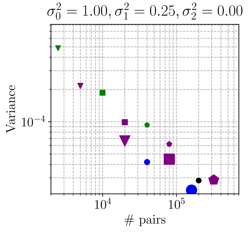
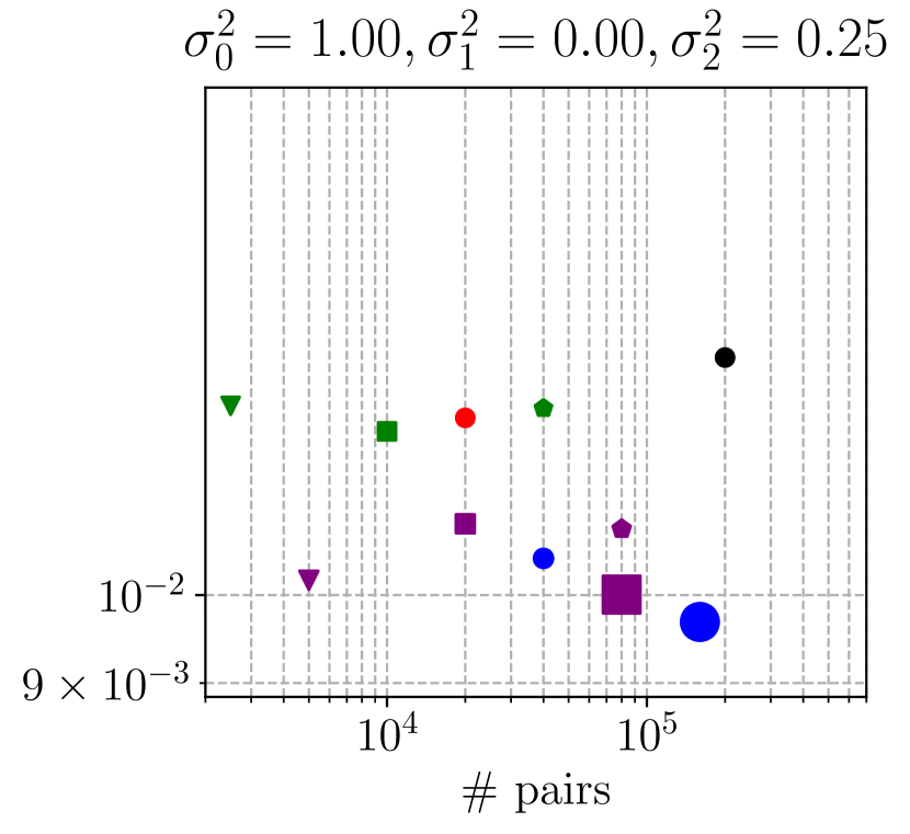
Figure 5: Empirical variances as a function of the number of evaluated pairs for SWOR, with $n=100,000$, $m=200$ and $N=100$, evaluated over 500 runs.

In this section, we numerically show that in practice, the results for SWOR do not deviate much from the theoretical ones obtained for prop-SWOR in Theorem 1 and Theorem 2. To illustrate this, we use the kernel $h(x,z)=x\cdot z$ and random variables in $\mathbb{R}$ that follow a normal law $X\sim\mathcal{N}(\mu_{X},\sigma_{X})$ and $Z\sim\mathcal{N}(\mu_{Z},\sigma_{Z})$. In that setting, note that $\sigma_{1}^{2}=\mu_{Z}^{2}\sigma_{X}^{2}$, $\sigma_{2}^{2}=\mu_{X}^{2}\sigma_{Z}^{2}$ and $\sigma_{0}^{2}=\sigma_{X}^{2}\sigma_{Z}^{2}$, which means that by tweaking the parameters $\mu_{X},\mu_{Z},\sigma_{X},\sigma_{Z}$, one can obtain any possible value of $\sigma_{1},\sigma_{2},\sigma_{0}$.

The results, shown in Fig. 5 are very similar to those obtained for prop-SWOR in Fig. 2. The fact that SWOR has slightly lower variance is expected, since when no pairs are available the default value is always 0. This makes the estimator give a stable prediction, but also makes it biased.

Appendix F Analysis of Proportional Sampling with Replacement (prop-SWR)

While the use of prop-SWR is not very natural in a standard distributed setting, it is relevant in cases where workers have access to joint database that they can efficiently subsample. We have the following results for the variance of estimates based on prop-SWR (see Section F.1 and Section F.2 for the proofs).

Theorem 3

If the data is distributed between workers with prop-SWR, and denoting $\mathbf{n}_{0}=(n/N,m/N)$, we have:

$$\text{Var}(U_{\mathbf{n},1}(h)) =\frac{\sigma_{1}^{2}}{n}\left(2-\frac{1}{n}\right)+\frac{\sigma_{2}^{2}}{m}\left(2-\frac{1}{m}\right)+\frac{\sigma_{0}^{2}}{nm}\left[4-2\left(\frac{1}{n}+\frac{1}{m}\right)+\frac{1}{nm}\right],$$

$$\text{Var}(U_{\mathbf{n},N}(h)) =\text{Var}(U_{\mathbf{n},1}(h))+\frac{\sigma_{0}^{2}}{nm}\left(N-1\right)\left(1-\frac{1}{n}\right)\left(1-\frac{1}{m}\right),$$

$$\text{Var}(\widetilde{U}_{\mathbf{n},N,B}(h)) =\text{Var}\left(U_{\textbf{n},N}(h)\right)+\frac{1}{NB}\left[\sigma^{2}-\text{Var}\left(U_{\mathbf{n}_{0},1}(h)\right)\right].$$

Theorem 4

If the data is distributed and repartitioned between workers with prop-SWR, we have:

$$\text{Var}(\widehat{U}_{\mathbf{n},N,T}(h)) =\text{Var}(U_{\mathbf{n}}(h))+\frac{1}{T}\left[\text{Var}(U_{\mathbf{n},N}(h))-\text{Var}(U_{\mathbf{n}}(h))\right],$$

$$\text{Var}(\widetilde{U}_{\mathbf{n},N,B,T}(h)) =\text{Var}\left(\widehat{U}_{\mathbf{n},N,T}(h)\right)+\frac{1}{NBT}\left[\sigma^{2}-\text{Var}(U_{\mathbf{n}_{0},1}(h))\right].$$

Fig. 6 gives a visual illustration of these results. First note that they are similar to those obtained for prop-SWOR in Fig. 2. Yet, the right-hand side figure shows that $\widetilde{U}_{\mathbf{n},N,B,T}$ can have a significantly lower variance than $\widehat{U}_{\mathbf{n},N,T}$, for the same number of evaluated pairs. This comes from the fact that $\widetilde{U}_{\mathbf{n},N,B,T}$ works on more bootstrap re-samples of the data than $\widehat{U}_{\mathbf{n},N,T}$, hence better correcting for the loss of information due to sampling with replacement (at the cost of more communication or disk reads). To stress this, we also represented $U_{\mathbf{n},1}$, i.e. the point that gives the variance of a complete estimator based on one bootstrap re-sample of the data.

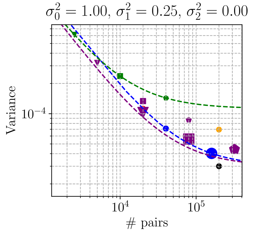
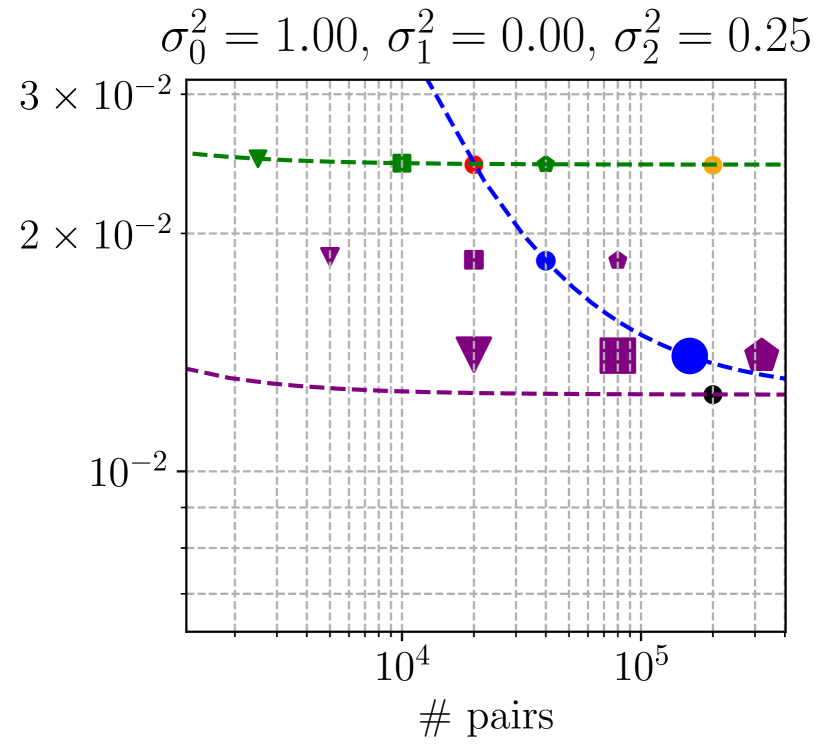
Figure 6: Theoretical variances as a function of the number of evaluated pairs for different estimators under prop-SWR, with $n=100,000$, $m=200$ and $N=100$.

F.1 Proof of Theorem 3

First we derive the variance of $U_{\mathbf{n},N}(h)$. Since $\mathbb{E}[U_{\mathbf{n},N}(h)|\mathcal{D}_{n},\mathcal{Q}_{m}]=U_{\mathbf{n}}(h)$, the law of total variance implies:

$$\text{Var}(U_{\mathbf{n},N}(h)) =\text{Var}(U_{\mathbf{n}}(h))+\mathbb{E}\left[\text{Var}\left(U_{\mathbf{n},N}(h)|\mathcal{D}_{n},\mathcal{Q}_{m}\right)\right],$$

$$=\text{Var}(U_{\mathbf{n}}(h))+\frac{1}{N}\mathbb{E}\left[\text{Var}\left(U_{\mathcal{R}_{1}}(h)|\mathcal{D}_{n},\mathcal{Q}_{m}\right)\right].$$

Introduce $\epsilon(k)$ (resp. $\gamma(l)$) as the random variable that is equal to the number of times that $k$ has been sampled in cluster $1$ for the $\mathcal{D}_{n}$ elements (resp. that $l$ has been sampled in cluster $1$ for the $\mathcal{Q}_{m}$ elements). The random variable $\epsilon(k)$ (resp. $\gamma(l)$) follows a binomial distribution with parameters $(n/N,1/n)$ (resp. $(m/N,1/m)$). Note that the $\epsilon$ and $\gamma$ are independent and that $\sum_{k=1}^{n}\epsilon(k)=n/N$ and $\sum_{l=1}^{m}\gamma(l)=m/N$. It follows that:

$$U_{\mathcal{R}_{1}}(h)-U_{n}(h)=U(h) +\frac{1}{n}\sum_{k=1}^{n}\left(N\epsilon(k)-1\right)\left(h_{1}(X_{k})-U(h)\right)$$

$$+\frac{1}{m}\sum_{l=1}^{m}\left(N\gamma(l)-1\right)\left(h_{2}(Z_{l})-U(h)\right)$$

$$+\frac{1}{nm}\sum_{k=1}^{n}\sum_{l=1}^{m}\left(N^{2}\epsilon(k)\gamma(l)-1\right)h_{0}(X_{k},Z_{l}),$$

which implies, using the results of Eq. 14,

$$\mathbb{E}\left[\text{Var}\left(U_{\mathcal{R}_{1}}(h)|\mathcal{D}_{n},\mathcal{Q}_{m}\right)\right] =\frac{N^{2}\sigma_{1}^{2}}{n}\text{Var}(\epsilon(1))+\frac{N^{2}\sigma_{2}^{2}}{m}\text{Var}(\gamma(1))+\frac{N^{4}\sigma_{0}^{2}}{nm}\text{Var}(\epsilon(1)\gamma(1)).$$ (17)

The mean and variance of a binomial distribution is known. Since $\epsilon(1)$ and $\gamma(1)$ are independent,

$$\begin{split}&\text{Var}(\epsilon(1)\gamma(1))=\frac{1}{N^{2}}\left[\left(1-\frac{1}{n}\right)\left(1-\frac{1}{m}\right)+\frac{1}{N}\left(2-\frac{1}{n}-\frac{1}{m}\right)\right],\\ &\text{Var}(\epsilon(1))=\frac{1}{N}\left(1-\frac{1}{n}\right),\quad\text{Var}(\gamma(1))=\frac{1}{N}\left(1-\frac{1}{m}\right).\end{split}$$ (18)

Plugging Eq. 18 into Eq. 17 gives the result. Explicitly,

$$\text{Var}\left(U_{\textbf{n},N}(h)\right)= \frac{\sigma_{1}^{2}}{n}\left(2-\frac{1}{n}\right)+\frac{\sigma_{2}^{2}}{m}\left(2-\frac{1}{m}\right)$$

$$+\frac{\sigma_{0}^{2}}{nm}\left[\left(3-\frac{1}{n}-\frac{1}{m}\right)+N\left(1-\frac{1}{n}\right)\left(1-\frac{1}{m}\right)\right].$$

Now we derive the variance of $\widetilde{U}_{\mathbf{n},N,B}(h)$. Note that $\mathbb{E}[\widetilde{U}_{\mathbf{n},N,B}|\mathcal{D}_{n},\mathcal{Q}_{m},\epsilon,\gamma]=U_{\mathbf{n},N}(h)$, hence:

Var $$(\widetilde{U}_{\mathbf{n},N,B})=\text{Var}(U_{\mathbf{n},N}(h))+\mathbb{E}\left[\text{Var}\left(\widetilde{U}_{\mathbf{n},N,B}|\mathcal{D}_{n},\mathcal{Q}_{m},\epsilon,\gamma\right)\right],$$

$$=\text{Var}(U_{\mathbf{n},N}(h))+\frac{1}{N}\mathbb{E}\left[\text{Var}\left(\widetilde{U}_{B,\mathcal{R}_{1}}|\mathcal{D}_{n},\mathcal{Q}_{m},\epsilon,\gamma\right)\right].$$ (19)

Conditioned upon $\mathcal{D}_{n},\mathcal{Q}_{m},\epsilon,\gamma$, the statistic $\widetilde{U}_{B,\mathcal{R}_{1}}$ is an average of $B$ independent experiments. Introducing $\delta_{k,l}$ as equal to $1$ if the pair $(k,l)$ is selected in worker $1$ as the $1$th pair of $\widetilde{U}_{B,\mathcal{R}_{1}}$, and $\Delta_{k,l}$ its expected value, i.e. $\Delta_{k,l}:=\mathbb{E}[\delta_{k,l}]=N^{2}\epsilon(k)\gamma(l)/nm$, it implies

Var $$\left(\widetilde{U}_{B,\mathcal{R}_{1}}\mid\mathcal{D}_{n},\mathcal{Q}_{m},\epsilon,\gamma\right)=\frac{1}{B}\text{Var}\left(\sum_{k=1}^{n}\sum_{l=1}^{m}\delta_{k,l}h(X_{k},Z_{l})\mid\mathcal{D}_{n},\mathcal{Q}_{m},\epsilon,\gamma\right).$$ (20)

From the definition of $\delta_{k,l}$ we have $\delta_{k,l}\delta_{k_{1},l_{1}}=0$ as soon as $k\neq k_{1}$ or $l\neq l_{1}$, writing the right-hand-side of Eq. 20 as the second order moment minus the squared means gives:

Var $$\left(\widetilde{U}_{B,\mathcal{R}_{1}}\mid\mathcal{D}_{n},\mathcal{Q}_{m},\epsilon,\gamma\right)=\frac{1}{B}\sum_{k=1}^{m}\sum_{l=1}^{n}\Delta_{k,j}h^{2}(X_{k},Z_{l})-\frac{1}{B}\left(\sum_{k=1}^{n}\sum_{l=1}^{m}\Delta_{k,l}h(X_{k},Z_{l})\right)^{2}.$$ (21)

Taking the expectation of Eq. 21 gives:

$$\mathbb{E}\Big{[}\text{Var}\left(\widetilde{U}_{B,\mathcal{R}_{1}}|\mathcal{D}_{n},\mathcal{Q}_{m},\epsilon,\gamma\right)\Big{]} =\frac{1}{B}\left[\mathbb{E}[h^{2}(X,Z)]-\mathbb{E}[U_{\mathcal{R}_{1}}^{2}]\right],$$

$$=\frac{1}{B}\left[\text{Var}(h(X,Z))-\text{Var}(U_{\mathcal{R}_{1}})\right].$$ (22)

Pluging Eq. 22 into Eq. 19 gives

$$\text{Var}(\widetilde{U}_{\mathbf{n},N,B}) =\frac{\text{Var}(h(X,Z))}{BN}+\text{Var}(U_{\mathbf{n},N}(h))-\frac{\text{Var}(U_{\mathcal{R}_{i}})}{BN},$$

and we can conclude from preceding results, since $U_{\mathcal{R}_{i}}$ is simply $U_{\mathbf{n}_{0},1}$ with $n_{0}=(n/N,m/N)$.

F.2 Proof of Theorem 4

Since $\mathbb{E}\left[\widehat{U}_{\mathbf{n},N,T}(h)|\mathcal{D}_{n},\mathcal{Q}_{m}\right]=U_{\mathbf{n}}(h)$ the law of total covariances followed by the fact that, conditioned upon $\mathcal{D}_{n},\mathcal{Q}$, the statistic $\widehat{U}_{\mathbf{n},N,T}(h)$ is an average of $T$ independent random variables, implies:

$$\text{Var}\left(\widehat{U}_{\mathbf{n},N,T}(h)\right)=\text{Var}(U_{\mathbf{n}}(h))+\frac{1}{T}\mathbb{E}\left[\text{Var}\left(U_{\mathbf{n},N}(h)|\mathcal{D}_{n},\mathcal{Q}_{m}\right)\right].$$

The calculations of Section F.2 give the result. Explicitly,

$$\text{Var}\left(\widehat{U}_{\mathbf{n},N,T}(h)\right) =\text{Var}(U_{\mathbf{n}}(h))+\frac{1}{T}\left[\text{Var}(U_{\mathbf{n},N}(h))-\text{Var}(U_{\mathbf{n}}(h))\right].$$

We now derive the variance of $\widetilde{U}_{\mathbf{n},N,B,T}$. Since

$$\mathbb{E}\left[\widetilde{U}_{\mathbf{n},N,B,T}(h)|\mathcal{D}_{n},\mathcal{Q}_{m},\epsilon,\gamma\right]=\widehat{U}_{\mathbf{n},N,T}(h),$$

the law of total covariance followed by the calculations of Section F.2 imply the result:

$$\text{Var}\left(\widetilde{U}_{\mathbf{n},N,B,T}(h)\right) =\text{Var}\left(\widehat{U}_{\mathbf{n},N,T}(h)\right)+\mathbb{E}\left[\text{Var}\left(\widetilde{U}_{\mathbf{n},N,B,T}(h)|\mathcal{D}_{n},\mathcal{Q}_{m},\epsilon,\gamma\right)\right],$$

$$=\text{Var}\left(\widehat{U}_{\mathbf{n},N,T}(h)\right)+\frac{1}{T}\mathbb{E}\left[\text{Var}\left(\widetilde{U}_{\mathbf{n},N,B}(h)|\mathcal{D}_{n},\mathcal{Q}_{m},\epsilon,\gamma\right)\right],$$

$$=\text{Var}\left(\widehat{U}_{\mathbf{n},N,T}(h)\right)+\frac{1}{NBT}\left[\text{Var}(h(X,Z))-\text{Var}(U_{\mathcal{R}_{i}})\right].$$

Appendix G Details on the Estimation Experiment of Section 5

Here we give some details on the derivations leading to Eq. 13. We have:

$$U(h) =\mathbb{P}\left(X>Z\right)=q+(1-q)(1-p),$$

$$h_{1}(x) =\mathbb{P}\left(x>Z\right)=1-p+p\cdot{\mathbb{I}}\{x=2\},$$

$$h_{2}(z) =\mathbb{P}\left(X>z\right)=q+(1-q){\mathbb{I}}\{z=-1\},$$

$$h_{0}(x,z) ={\mathbb{I}}\{x=2\}+{\mathbb{I}}\{x=0\}\cdot{\mathbb{I}}\{z=-1\}-h_{1}(x)-h_{2}(z)+U(h),$$

$$=-\left({\mathbb{I}}\left\{X=2\right\}-q\right)\left({\mathbb{I}}\left\{Z=-1\right\}-(1-p)\right).$$

It follows that:

$$\sigma_{1}^{2} =p^{2}q(1-q),$$

$$\sigma_{2}^{2} =(1-q)^{2}p(1-p),$$

$$\sigma_{0}^{2} =pq(1-p)(1-q).$$

References

- [1] Y. Arjevani and O. Shamir. Communication complexity of distributed convex learning and optimization. In NIPS, 2015.
- [2] M.-F. Balcan, A. Blum, S. Fine, and Y. Mansour. Distributed Learning, Communication Complexity and Privacy. In COLT, 2012.
- [3] R. Bekkerman, M. Bilenko, and J. Langford. Scaling Up Machine Learning: Parallel and Distributed Approaches. Cambridge University Press, 2011.
- [4] A. Bellet, Y. Liang, A. B. Garakani, M.-F. Balcan, and F. Sha. A Distributed Frank-Wolfe Algorithm for Communication-Efficient Sparse Learning. In SDM, 2015.
- [5] P. Bertail and J. Tressou. Incomplete generalized U-statistics for food risk assessment. Biometrics, 62(1):66–74, 2006.
- [6] G. Blom. Some properties of incomplete -statistics. Biometrika, 63(3):573–580, 1976.
- [7] L. Bottou and O. Bousquet. The Tradeoffs of Large Scale Learning. In NIPS, 2007.
- [8] S. P. Boyd, N. Parikh, E. Chu, B. Peleato, and J. Eckstein. Distributed Optimization and Statistical Learning via the Alternating Direction Method of Multipliers. Foundations and Trends in Machine Learning, 3(1):1–122, 2011.
- [9] S. Bubeck. Convex Optimization: Algorithms and Complexity. Foundations and Trends in Machine Learning, 8(3–4):231–357, 2015.
- [10] P. Carbone, A. Katsifodimos, S. Ewen, V. Markl, S. Haridi, and K. Tzoumas. Apache Flink™: Stream and Batch Processing in a Single Engine. IEEE Data Engineering Bulletin, 38(4):28–38, 2015.
- [11] S. Clémençon. A statistical view of clustering performance through the theory of U-processes. Journal of Multivariate Analysis, 124:42–56, 2014.
- [12] S. Clémençon, A. Bellet, and I. Colin. Scaling-up Empirical Risk Minimization: Optimization of Incomplete U-statistics. Journal of Machine Learning Research, 13:165–202, 2016.
- [13] S. Clémençon, G. Lugosi, and N. Vayatis. Ranking and empirical risk minimization of -statistics. The Annals of Statistics, 36(2):844–874, 2008.
- [14] S. Clémençon and S. Robbiano. Building confidence regions for the ROC surface. Pattern Recognition Letters, 46:67–74, 2014.
- [15] H. Daumé III, J. M. Phillips, A. Saha, and S. Venkatasubramanian. Protocols for Learning Classifiers on Distributed Data. In AISTATS, 2012.
- [16] V. de la Pena and E. Giné. Decoupling: from Dependence to Independence. Springer, 1999.
- [17] J. Dean and S. Ghemawat. Mapreduce: simplified data processing on large clusters. Communications of the ACM, 51(1):107–113, 2008.
- [18] W. Hoeffding. A class of statistics with asymptotically normal distribution. Annals of Mathematics and Statistics, 19:293–325, 1948.
- [19] M. Jordan. On statistics, computation and scalability. Bernoulli, 19(4):1378–1390, 2013.
- [20] A. Lee. -statistics: Theory and practice. Marcel Dekker, Inc., New York, 1990.
- [21] G. Papa, A. Bellet, and S. Clémençon. SGD Algorithms based on Incomplete U-statistics: Large-Scale Minimization of Empirical Risk. In NIPS, 2015.
- [22] V. Smith, S. Forte, C. Ma, M. Takác, M. I. Jordan, and M. Jaggi. CoCoA: A General Framework for Communication-Efficient Distributed Optimization. Journal of Machine Learning Research, 18(230):1–49, 2018.
- [23] A. Van Der Vaart. Asymptotic Statistics. Cambridge University Press, 2000.
- [24] R. Vogel, A. Bellet, and S. Clémençon. A Probabilistic Theory of Supervised Similarity Learning for Pointwise ROC Curve Optimization. In ICML, 2018.
- [25] E. P. Xing, Q. Ho, W. Dai, J. K. Kim, J. Wei, S. Lee, X. Zheng, P. Xie, A. Kumar, and Y. Yu. Petuum: A New Platform for Distributed Machine Learning on Big Data. IEEE Transactions on Big Data, 1(2):49–67, 2015.
- [26] M. Zaharia, M. Chowdhury, M. J. Franklin, S. Shenker, and I. Stoica. Spark : Cluster Computing with Working Sets. In HotCloud, 2012.