Comparison of MPS based real time evolution algorithms for Anderson Impurity Models

Abstract

We perform a detailed comparison of two Matrix Product States (MPS) based time evolution algorithms for Anderson Impurity Models. To describe the bath, we use both the star-geometry as well as the commonly employed Wilson chain geometry. For each bath geometry, we use either the Time Dependent Variational Principle (TDVP) or the Time Evolving Block Decimation (TEBD) to perform the time evolution. To apply TEBD for the star-geometry, we use a specially adapted algorithm that can deal with the long-range coupling terms. Analyzing the major sources of errors, one expects them to be proportional to the system size for all algorithms. Surprisingly, we find errors independent of system size except for TEBD in chain geometry. Additionally, we show that the right combination of bath representation and time evolution algorithm is important. While TDVP in chain geometry is a very precise approach, TEBD in star geometry is much faster, such that for a given accuracy it is superior to TDVP in chain geometry. This makes the adapted version of TEBD in star geometry the most efficient method to solve impurity problems.

I Introduction

Describing strongly correlated electron materials is among the most difficult tasks in solid state physics. One breakthrough in this field was the development of the Dynamical Mean Field Theory (DMFT) Metzner and Vollhardt (1989); Georges and Kotliar (1992); Georges et al. (1996). DMFT accounts for local electronic correlations by a self-consistent mapping of a lattice problem, describing the low-energy subspace of the material, onto an Anderson Impurity Model (AIM) Anderson (1961). The subsequent solution of this impurity problem is the most important part of a DMFT calculation. At present, Continuous Time Quantum Monte Carlo (CTQMC) Werner et al. (2006); Gull et al. (2011) is the work-horse method for DMFT real material calculations. Many other approaches exist, like the Numerical Renormalization Group Wilson (1975); Bulla et al. (2008), Configuration Interaction Lu et al. (2014); Zgid et al. (2012); Mejuto Zaera et al. (2017), and also methods based on the Density Matrix Renormalization Group (DMRG) and the related Matrix Product States (MPS) White (1992); Schollwöck (2011).
One of the major advantages of MPS based impurity solvers is that they can give access to real-frequency spectral functions by employing real-time evolution. While these methods provide excellent results for the single orbital case, adding more and more orbitals is a very challenging task. To overcome this issue, the Fork Tensor Product States (FTPS) Bauernfeind et al. (2017) solver was recently developed and applied to several materials Bauernfeind et al. (2017, 2018). This new approach has allowed to resolve multiplets in the Hubbard bands of the single particle excitation spectrum for real materials, which have also been observed experimentally Bauernfeind et al. (2018) but are inaccessible from the imaginary time results from standard CTQMC methods. It is therefore important to identify the most efficient methods for real-time evolution of impurity models.

A recent review Paeckel et al. (2019) reported an extensive comparison of several MPS-based time evolution algorithms for different types of models. It did not, however, include impurity problems. They are special in the sense that most of the degrees of freedom are non-interacting. The conclusion of Ref. Paeckel et al., 2019 was that methods perform better or worse depending on the model or observable studied. In all cases, the Time Dependent Variational Principle (TDVP) Haegeman et al. (2011, 2016) was among the most reliable approaches, while the global Krylov method although accurate tended to be too time-consuming.

Using tensor networks, impurity problems usually have been transformed to the Wilson chain-geometry representation of the bath - essentially a nearest neighbor tight-binding chain. The so-called star geometry on the other hand involves hopping processes from the impurity to all bath sites that become long ranged when mapped onto a linear chain. Although the reformulation of DMRG as a variational principle on the space of MPS allows to deal with such long-range terms, the chain geometry was believed to be the superior representation of impurity models. Surprisingly, Wolf et al. Wolf et al. (2014) demonstrated that for MPS, the star geometry is in fact a more economic representation. Wolf et al. used the global Krylov method to perform the time evolution which can be, as mentioned above, very time-consuming. As an alternative, some of us published a modified Time Evolving Block Decimation (TEBD)  Vidal (2003, 2004); Daley et al. (2004) algorithm for the star geometry in Ref. Bauernfeind et al., 2017. There is also the possibility to use the TDVP, which has been argued to be suited to long-range terms  Haegeman et al. (2011). Therefore, open questions remain regarding the time evolution methods used for impurity problems, for example: Does the bath geometry affect the accuracy of the result? If so, does this depend on the time evolution algorithm? And arguably the most important one: Which method is best?

In the present paper, we use TDVP and TEBD as time evolution algorithms for AIMs in the star and chain geometry and perform an in-depth comparison of the four possibilities. We compare the quantity of interest in DMFT calculations, i.e., the impurity Green’s function. We show that to obtain precise results, the correct combination of bath representation and time evolution algorithm is crucial. Specifically we demonstrate that the adapted TEBD Vidal (2003, 2004); Daley et al. (2004) is more accurate in the star geometry, while TDVP gives better results in the chain geometry. We find that the TEBD approach in star-geometry is much faster than TDVP in the chain geometry when a specific precision of the Green’s function is prescribed. Additionally, we focus on the behavior of the algorithms as a function of bath size. Surprisingly, all algorithms except TEBD in chain-geometry have errors nearly independent of system size. This very favorable scaling is especially important for DMFT calculations, as one wants to use a large number of sites to represent the bath hybridization well.

This paper is structured as follows. In Sec. II we introduce AIMs in star-geometry and in chain-geometry representation of the bath and discuss how to obtain bath parameters from the bath hybridization. In Sec. III, we briefly introduce MPS and how to obtain Green’s functions using real-time evolution. In Sec. IV we discuss the different time evolution methods, including a discussion of the various error sources. Sec. V contains results, first for the non-interacting case, and in Sec. V.2 for the interacting case. Finally, Sec. VI contains the conclusions.

II Anderson Impurity Models

In the star geometry, an impurity described by a local interacting Hamilton ${H_{\text{loc}}}$ is coupled to a bath of free fermions via hopping terms from the impurity to every bath site. For a one-band model this results in:

$$H_{\text{star}} =H_{\text{loc}}+H_{\text{bath}}$$ (1)

$$H_{\text{loc}} =Un_{I,\uparrow}n_{I,\downarrow}+\epsilon_{I}\left(n_{I,\uparrow}+n_{I,\downarrow}\right)$$

$$H_{\text{bath}} =\sum_{k,\sigma}H_{k,\sigma}=\sum_{k,\sigma}\epsilon_{k}n_{k,\sigma}+V_{k}\left(c^{\dagger}_{I,\sigma}c_{k,\sigma}+c^{\dagger}_{k,\sigma}c_{I,\sigma}\right).$$

Here, $c_{k,\sigma}^{\dagger}$ $(c_{k,\sigma})$ create (annihilate) an electron at bath site $k$ with spin $\sigma$, $n_{k,\sigma}=c^{\dagger}_{k,\sigma}c_{k,\sigma}$ are the usual particle number operators and we label the impurity degrees of freedom by an index $I$. If one puts the sites of $H_{\text{star}}$ on a one-dimensional manifold (like an MPS - see below), the hopping terms become long-range.
 
Using a Lanzcos-like tridiagonalization, one can map the star geometry onto the so-called Wilson chain Wilson (1975); Bulla et al. (2008) or just chain-geometry, where the impurity couples to the first bath site only:

$$H_{\text{chain}} ={H_{\text{loc}}}+t_{0}\left(c^{\dagger}_{I,\sigma}c_{1,\sigma}+c^{\dagger}_{1,\sigma}c_{I,\sigma}\right)+$$ (2)

$$\sum_{i,\sigma}t_{i}\left(c^{\dagger}_{i,\sigma}c_{i+1,\sigma}+c^{\dagger}_{i+1,\sigma}c_{i,\sigma}\right)+\bar{\epsilon}_{i}n_{i\sigma}.$$

II.1 Determination of Bath parameters

The bath can also be described by the continuous (DMFT Georges et al. (1996)) hybridization function $\Delta(\omega)$. By tracing out the bath in Eq. (1), one finds:

$$\Delta(\omega) =\sum_{k}\frac{V_{k}^{2}}{\omega-\epsilon_{k}+i0^{+}}$$ (3a)

$$-\frac{1}{\pi}\mathcal{I}\Delta(\omega) \approx\sum_{k=1}^{N}V_{k}^{2}\frac{\eta}{\pi\left(\left(\omega-\epsilon_{k}\right)^{2}+\eta^{2}\right)}.$$ (3b)

A continuous bath corresponds to an infinite sum. In the last line, we used only a finite number of $N$ bath sites, and approximated the delta-peaks by Lorentzians of finite width $\eta$. Usually, the hybridization function $\Delta(\omega)$ is given and in order to map it to an AIM of finite size, one needs to find values $\epsilon_{k}$ and $V_{k}$, such that Eq. (3b) is as good approximation. In the present study, we choose to split the $\omega$-axis into $N$ equidistant intervals $I_{k}$ of size $\Delta\epsilon$. We describe each interval using a single bath site with on-site energy $\epsilon_{k}=\min I_{k}+\frac{\Delta\epsilon}{2}$, where $\min I_{k}$ is the minimum of interval $I_{k}$. The hopping amplitude $V_{k}$ can then be computed from Bulla et al. (2008); Wolf et al. (2014):

$$V_{k}^{2}=\int_{I_{k}}-\frac{1}{\pi}\mathcal{I}\Delta(\omega).$$ (4)

A subsequent basis transformation into the Lanzcos-basis of ${H_{\text{bath}}}$ yields the bath parameters in the chain geometry Bulla et al. (2008); Wolf et al. (2014). Note that for particle hole symmetry, the on-site energies $\bar{\epsilon}_{i}$ of the chain geometry are exactly zero Bulla et al. (2008). For both geometries, we enforce particle hole symmetry in the bath parameters. In the following, we will give all results in units of the half bandwidth of the bath spectral function $-\frac{1}{\pi}\mathcal{I}\Delta(\omega)$.

III Matrix Product States

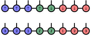
Figure 1: Graphical representation of an MPS used for an AIM with $N=3$ bath sites. Top: To separate the spin species, we place the impurity in the middle (green circles) and attach the spin-up (spin-down) bath to the left (right) colored in blue (red). Bottom: Labeling of sites in the star- as well as in the chain-geometry. The bath sites are arranged in ascending order with increasing distance from the impurity.

MPS are an efficient parametrization of quantum mechanical states as a product of local matrices. Consider a system consisting of $2N+2$ sites with a local basis $\ket{s_{i}}$ at site $i$:

$$\ket{\psi}=\sum_{\{s\}}c_{s_{1},\cdots s_{2N+2}}\ket{s_{1}\cdots s_{2N+2}}.$$ (5)

In an MPS, the coefficient $c_{s_{1},\cdots s_{2N+2}}$ is factorized into a product of matrices using repeated Singular Value Decompositions (SVDs) Schollwöck (2011):

$$c_{s_{1},\cdots s_{2N+2}}=A^{s_{1}}\cdot A^{s_{2}}\cdots A^{s_{2N+1}}.$$ (6)

Each $A_{i}^{s_{i}}$ is a rank-$3$ tensor, except the two tensors at the edges which are of rank-$2$. Since $s_{i}$ represents the local basis $\ket{s_{i}}$, this index is called physical. The matrix indices which are summed over are called bond-indices. The dimension of the bond indices (bond dimension) is the number of Schmidt values kept during the calculation, implying that some Schmidt values are discarded. The sum of the square of all discarded Schmidt values is called truncated weight $t_{w}$ Schollwöck (2011). MPS and other tensor networks are often depicted using a graphical representation as in Fig. 1. Since the Hamiltonian of an AIM connects the two spin species only via interactions on the impurity (see Eq. (1)), it has turned out to be favorable to separate them in the MPS, and to use a local Hilbert space of dimension two (empty and occupied) for each site Saberi et al. (2008); Ganahl et al. (2015); Bauernfeind et al. (2017). Thus, we place the impurity in the middle of the chain and connect the spin-up (spin-down) bath to its left (right), as shown in Fig. 1.
Using this arrangement of sites, we calculate the ground state $\ket{\psi_{0}}$ and its energy $E_{0}$ using DMRG. The central object of interest in DMFT calculations is the Green’s function of the impurity. In the following, we will hence focus our attention on the greater Green’s function of the impurity (omitting the spin index):

$$G^{>}(t) =\bra{\psi_{0}}c_{I}e^{-iHt}c_{I}^{\dagger}\ket{\psi_{0}}e^{iE_{0}t}$$ (7)

$$=\left(e^{iH\frac{t}{2}}c_{I}^{\dagger}\ket{\psi_{0}}\right)^{\dagger}\left(e^{-iH\frac{t}{2}}c_{I}^{\dagger}\ket{\psi_{0}}\right)e^{iE_{0}t}.$$

To calculate Eq. (7), we first apply the operator $c^{\dagger}_{I}$ onto the ground state. Next, as indicated by brackets in the the second line of Eq. (7), we perform two separate time evolutions up to time $\frac{t}{2}$ Ganahl et al. (2015); Kennes and Karrasch (2016) and calculate the overlap. We checked that the results are the same for the lesser Green’s function and also checked that non-particle hole symmetric models show a behavior very similar to the results presented below.

IV Time Evolution Algorithms

In the following, we discuss the different time evolution algorithms with special attention to our adapted TEBD approach in star geometry, and we analyze the main sources of error.

IV.1 TEBD

Several slightly different formulations of TEBD Vidal (2003, 2004); Daley et al. (2004); Paeckel et al. (2019) exist. The common strategy is to split the full time evolution operator of some small time step $\tau$ into manageable parts which can be applied to evolve the state forward in time. Specifically, one employs Suzuki-Trotter breakups Suzuki (1990) to obtain a decomposition into operators acting on two sites only. The action of such a gate merges the MPS tensors of the two sites, which are then separated again using a SVD combined with a truncation. Apart from the truncation, the main error of this approach is caused by the (in our case second order) Trotter breakup:

$$e^{\tau(A+B)} =e^{-iA\frac{\tau}{2}}e^{-iB\tau}e^{-iA\frac{\tau}{2}}+\frac{\tau^{3}}{12}\mathcal{C}+\mathcal{O}(\tau^{4})$$ (8)

$$\mathcal{C} =\left(\frac{1}{2}\big{[}A,[A,B]\big{]}+\big{[}B,[A,B]\big{]}\right).$$

According to Eq. (8), the total error of the time evolution is not only determined by the time step $\tau$, but also by the matrix elements of the double commutators $\mathcal{C}$. Since the latter are different for the star and the chain geometry, the error of TEBD in both geometries can be very different. This will be discussed in the following two subsections.

Chain Geometry

To employ TEBD in the chain-geometry, we use the standard second order breakup between even and odd terms Schollwöck (2011). We write the Hamiltonian of the chain geometry $H_{\text{chain}}=\sum_{i}h_{i,i+1}$ as a sum of local terms $h_{i,i+1}$ acting on nearest neighbor sites $i$ and $i+1$ only and define:

$$H_{\text{chain}} =H_{\text{even}}+H_{\text{odd}}$$

$$H_{\text{even}} =\sum_{i:\text{even}}h_{i,i+1}\text{, }$$

$$H_{\text{odd}} =\sum_{i:\text{odd}}h_{i,i+1}$$

$$e^{-iH_{\text{chain}}{\Delta t}} \approx e^{-iH_{\text{odd}}\frac{{\Delta t}}{2}}e^{-iH_{\text{even}}{\Delta t}}e^{-iH_{\text{odd}}\frac{{\Delta t}}{2}}.$$ (9)

In the particle hole symmetric case, the on-site energies $\bar{\epsilon_{i}}$ are exactly zero, removing any ambiguity of how to distribute the on-site terms among even- and odd parts of the Hamiltonian. For particle hole symmetry ($\bar{\epsilon_{i}}=0$), we evaluated the double commutators of Eq. (8). They turn out to be various sums over hopping terms multiplied by three amplitudes:

$$\mathcal{C}_{\text{chain}}=-\frac{1}{2}\sum_{i:\text{even}}t_{i}t_{i+1}t_{i+2}\left(c^{\dagger}_{i}c_{i+3}+c^{\dagger}_{i+3}c_{i}\right)+\cdots.$$ (10)

Additionally, the interaction $U$ gives two terms that couple to the neighbors of the impurity, independent of $N$. For the scaling with bath size the latter terms can be neglected, since they are of order $\mathcal{O}(1)$. Each of the individual sums of Eq. 10 scales linearly with system size $N$, they contain $N$ terms of order $1$, and the hopping amplitudes $t_{i}$ are independent of $N$ . Thus, one should expect the overall error of TEBD in chain geometry to scale like the bath size $N$.

Star Geometry

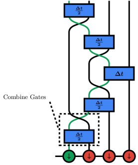
Figure 2: Application of the time evolution operator of Eq. (12) onto the spin-down bath. We use swap gates depicted by two crossing arcs to evolve the long-range hopping terms. The green line visualizes the position of the impurity as it is moved through the bath during the time evolution. All gates except the one with $H_{N,\sigma}$ are calculated with a time step $\frac{{\Delta t}}{2}$, reflecting the use of the second order breakup. Note that with this approach one can combine every swap gate with an actual time evolution gate, thus avoiding any additional SVDs.

To perform the TEBD time evolution of an AIM in star geometry (Eq (1)), we employ an approach we recently developed (see Refs Bauernfeind et al., 2017; Bauernfeind, 2018), which is based on swap-gates Orús (2014); Verstraete et al. (2009) and iterative Suzuki-Trotter decompositions. First, we first split off ${H_{\text{loc}}}$ from the time evolution operator for some small time-step ${\Delta t}$ in a second order Trotter decomposition:

$$e^{-iH{\Delta t}}\approx e^{-i{H_{\text{loc}}}\frac{{\Delta t}}{2}}\left(\prod_{\sigma}e^{-i\sum_{k}H_{k,\sigma}{\Delta t}}\right)e^{-i{H_{\text{loc}}}\frac{{\Delta t}}{2}},$$ (11)

where $H_{k,\sigma}$ was defined in Eq. (1). Then we split off the term containing $H_{1,\sigma}$, then $H_{2,\sigma}$ and so on, until we obtain:

$$e^{-i\sum_{k}H_{k,\sigma}{\Delta t}}\approx\left(\prod_{k=1}^{N}e^{-iH_{k,\sigma}\frac{{\Delta t}}{2}}\right)\left(\prod_{k=N}^{1}e^{-iH_{k,\sigma}\frac{{\Delta t}}{2}}\right).$$ (12)

The Trotter errors of these approximations will be discussed below. Note that Eq. (12) is a product of operators acting on two sites only, but all terms except $H_{1,\sigma}$ involve sites that are not nearest neighbors in the MPS. To be able to apply such non-nearest neighbor gates, we use swap-gates. Their purpose is to swap the degrees of freedom of two sites in the MPS-tensor network. For a fermionic Hilbert space with local dimension of $2$ (empty $\ket{0}$ or occupied $\ket{1}$), a swap-gate $S$ is given by:

$$S=\ket{00}\bra{00}+\ket{01}\bra{10}+\ket{10}\bra{01}-\ket{11}\bra{11}.$$ (13)

Note the minus sign in the last term, resulting from the exchange of two fermions Bauernfeind (2018). The process of applying all the gates in Eq. (12) is depicted in Fig. 2 and described in the following.

Instead of a gate with $H_{1,\sigma}$ only, we apply a combined gate $S\cdot e^{-iH_{1,\sigma}\frac{{\Delta t}}{2}}$, meaning that we first time evolve and swap afterwards. The impurity degrees of freedom are then located at what was previously the first bath site and is now a nearest neighbor of the second bath site. We continue by applying a combined two-site gate $S\cdot e^{-iH_{2,\sigma}\frac{{\Delta t}}{2}}$ after which the impurity and bath site $3$ are nearest neighbors and so on. When the impurity arrives at site $N-1$, we time evolve with $H_{N,\sigma}$ (without swapping). Since we used a second order decomposition, we have to re-apply all gates with $k=N-1\cdots 1$. This time, though, we have to swap first and time evolve afterwards, since otherwise we would have to take care of an additional fermionic sign in the hopping terms Bauernfeind (2018). This means that we apply a two-site gate $e^{-iH_{N-1,\sigma}\frac{{\Delta t}}{2}}\cdot S$ followed by $e^{-iH_{N-2,\sigma}\frac{{\Delta t}}{2}}\cdot S$, etc., until the impurity is back in the middle of the MPS and every term in Eq (12) is dealt with.
 
Now let us evaluate the Trotter errors due to these various decompositions. In the first breakup, we split off ${H_{\text{loc}}}$ from the rest of the Hamiltonian, i.e., $A={H_{\text{loc}}}$ and $B={H_{\text{bath}}}$ in Eq. (8). Evaluation of the double commutators yields:

$$\mathcal{C}_{{H_{\text{loc}}}}=-2\sum_{\sigma}K_{\sigma}n_{I,\sigma}\sum_{k}V_{k}^{2}$$ (14)

$$+\sum_{k,\sigma}V_{k}\left(c^{\dagger}_{I,\sigma}c_{k,\sigma}+c^{\dagger}_{k,\sigma}c_{I,\sigma}\right)K_{\sigma}\left(\frac{1}{2}K_{\sigma}-\epsilon_{k}\right)$$

$$+\sum_{k,k^{\prime},\sigma}V_{k}V_{k^{\prime}}K_{\sigma}\left(c^{\dagger}_{k,\sigma}c_{k^{\prime},\sigma}+c^{\dagger}_{k^{\prime},\sigma}c_{k,\sigma}\right)$$

$$-\sum_{k,k^{\prime},\sigma}V_{k}V_{k^{\prime}}U\left(c^{\dagger}_{I,\sigma}c_{k^{\prime},\sigma}-c^{\dagger}_{k^{\prime},\sigma}c_{I,\sigma}\right)\left(c^{\dagger}_{I,\bar{\sigma}}c_{k,\bar{\sigma}}-c^{\dagger}_{k,\bar{\sigma}}c_{I,\bar{\sigma}}\right),$$

with $K_{\sigma}=Un_{I\bar{\sigma}}+\epsilon_{0}$ and $\bar{\sigma}$ the spin in opposite direction of spin $\sigma$.
Next, we split off $H_{1,\sigma}$ from $\sum_{k>1}H_{k,\sigma}$, i.e., $A=H_{1,\sigma}$ and $B=\sum_{k>1}H_{k,\sigma}$. The error of this decomposition (with $j=1$):

$$\mathcal{C}_{H_{j,\sigma}} =\frac{1}{2}\sum_{k>j}V_{j}^{2}V_{k}\left(c^{\dagger}_{I,\sigma}c_{k,\sigma}+c^{\dagger}_{k,\sigma}c_{I,\sigma}\right)$$ (15)

$$-V_{j}\left(c^{\dagger}_{I,\sigma}c_{j,\sigma}+c^{\dagger}_{j,\sigma}c_{I,\sigma}\right)\sum_{k>j}V_{k}^{2}$$

$$+\sum_{k>j}V_{j}V_{k}\left(c^{\dagger}_{j,\sigma}c_{k,\sigma}+c^{\dagger}_{k,\sigma}c_{j,\sigma}\right)\left(\frac{1}{2}\epsilon_{j}-\epsilon_{k}\right).$$

The next decomposition separating $H_{2,\sigma}$ from $\sum_{k>2}H_{k,\sigma}$ has the exact same form as above now with $j=2$, and hence an error of $\mathcal{C}_{H_{j,\sigma}}$ for $j=2$. Iterating over all decompositions, the total error of the breakup used to separate the time evolution operator in the star geometry becomes:

$$\mathcal{C}_{\text{star}}=\mathcal{C}_{H_{\text{loc}}}+\sum_{j\neq N,\sigma}\mathcal{C}_{H_{j,\sigma}}.$$ (16)

Let us analyze how this error scales with the number of bath sites $N$. From Eq. (3a), we find that $V_{k}\sim\frac{1}{\sqrt{N}}$. Hence, $\mathcal{C}_{H_{\text{loc}}}$ in Eq. (14) scales linearly with $N$, since each of the last two lines contains $N^{2}$ terms of order $1$ multiplied by $V_{k}^{2}\sim\frac{1}{N}$.
Similarly, the other terms in Eq.16 give a growth of the error not faster than $N$ (two terms in $\mathcal{C}_{H_{\text{loc}}}$ also have $\sim N$ scaling and the next lowest order is a $\sqrt{N}$-scaling). We hence should expect the error in the star geometry to scale linearly with $N$.
This might seem surprising at first, since to obtain Eq. (12), we performed $N$ individual decompositions and one might therefore expect the total error to scale at least $\sim N^{2}$. However, since the hopping parameters are $N$-dependent themselves ($V_{k}\sim\frac{1}{\sqrt{N}}$), the overall error improves by a factor of $\frac{1}{N}$. Note that the actual errors in the calculations will depend on the matrix elements of the error terms Eq.(10) or Eq. (16).

IV.2 TDVP

Instead of approximating the time evolution operator, TDVP directly solves the time dependent Schrödinger equation, albeit only in a restricted subspace - in the space of MPS of fixed bond dimension. TDVP constructs a projection operator $P_{T_{\ket{\psi}}}$ that projects the right hand side of the Schrödinger equation onto the tangent space $T_{\ket{\psi}}$ of the current MPS $\ket{\psi}$:

$$\frac{\partial}{\partial t}\ket{\psi}=-iP_{T_{\ket{\psi}}}H\ket{\psi}.$$ (17)

This equation then results in a set of equations that can be integrated with an approach very similar to DMRG, replacing the ground-state search by Krylov time propagation Haegeman et al. (2016); Paeckel et al. (2019). In the present publication we employ two-site TDVP (2TDVP in Ref. Paeckel et al., 2019) using the second order integrator by sweeping left-right-left with half time step $\frac{\Delta t}{2}$. For additional details on TDVP we refer to the existing literature Haegeman et al. (2011, 2016); Paeckel et al. (2019). Apart from MPS-matrix truncation and finite time step $\Delta t$, TDVP has an additional parameter, namely when to terminate the Krylov series. We stop creating new Krylov vectors when the total contribution of two consecutive vectors to the matrix exponential is less than $10^{-15}$.

The errors of TDVP are, apart from the truncation, a time step error similar to TEBD of order $\Delta t^{3}$ and an error due to the projection of the Schrödinger equation Paeckel et al. (2019). We expect the latter to strongly depend on the bath representation, because it is exactly zero for Hamiltonians with nearest neighbor terms only Paeckel et al. (2019); Haegeman et al. (2016). As a function of bath size, we expect an error linear in $N$, since TDVP approximates $N$ coupled equations by integrating them one after the other.

V Results

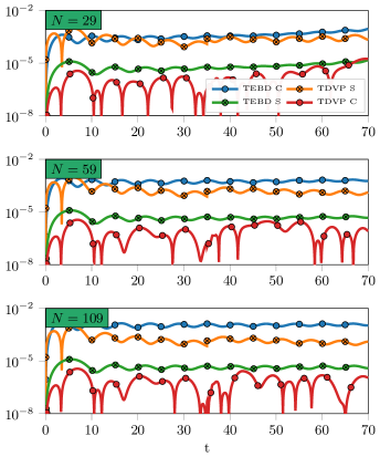
Figure 3: Absolute differences $|\Re G^{>}_{\text{exact}}(t)-\Re G^{>}_{\text{DMRG}}(t)|$ for chain- (C) and star (S) geometries and various bath sizes ($N=29,59,109$ from top to bottom) at $U=0$. The bath for this calculation was obtained from a semi-circular spectral function $-\frac{1}{\pi}\mathcal{I}\Delta(\omega)=\frac{1}{2\pi}\sqrt{1-\omega^{2}}$. The Trotter time-step was ${\Delta t}=0.05$. The truncated weight was set to $10^{-12}$ during DMRG as well as during time evolution and the bond dimensions were not restricted to any maximal value.

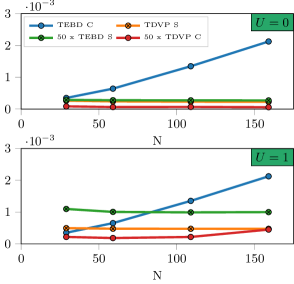
Figure 4: Maximum error for times $20<t<30$ as a function of bath size. Top: $U=0$ calculation shown in Fig. 3. Bottom: $U=1$ calculation shown in Fig. 6. Note that the errors of TEBD-S and TDVP-C have been multiplied by a factor of 50 to make the graphs comparable.

To compare the different algorithms which have different sources of errors, we use the following strategy. We first fix the parameters (time step $\Delta t$ and truncated weight $t_{w}$) and compare the error of the Green’s function without taking the computation time into account. In the next step, we then address the real question of computation time versus error.

V.1 U=0

Since interactions only affect the impurity degrees of freedom, it is reasonable to expect that most of the errors from the approximations in the time evolution is already present in the non-interacting case. Starting with $U=0$ has the advantage of giving us access to the exact Green’s function by diagonalization of the hopping matrix $T_{ij}$:

$$H=\sum_{ij}c^{\dagger}_{i}T_{ij}c_{j}=\sum_{ijk}\underbrace{c^{\dagger}_{i}U^{\dagger}_{ik}}_{c^{\dagger}_{k}}E_{k}\underbrace{U_{kj}c_{j}}_{c_{k}}=\sum_{k}E_{k}n_{k},$$ (18)

where $H=H_{\text{star}}$ or $H=H_{\text{chain}}$, respectively. Note that in the following, we compare each calculation to the exact Green’s function for the system defined by its hopping matrix $T_{ij}$ for the finite size bath.
In Fig. 3 we compare the four time evolution schemes for various system sizes and for fixed parameters $\Delta t$ and truncation. The truncated weight was chosen very small ($10^{-12}$), such that the main error source is the approximation of the time evolution operator, not the truncation of the tensor network. The magnitude of the error suggests that TDVP in chain geometry (TDVP-C) is the best algorithm followed by the TEBD in star geometry (TEBD-S). This does not consider the necessary bond dimension $m$ though, which was very different depending mostly on the bath geometry. While in star geometry the bond dimensions were $48$ and $62$ for TDVP and TEBD respectively, they grew to $145$ and $220$ in chain geometry. This difference has drastic effects on the computation time discussed below, which scales $\sim m^{3}$.
Three observations are especially interesting in Fig. 3. First, for TDVP the chain geometry gives more precise results, whereas for TEBD the star geometry gives a lower error. For TDVP this behavior may be related to the projection error being zero in the chain geometry Haegeman et al. (2016).

Second, in all cases, the error seems to be about constant in time. This is true until the particle added in the calculation of the Green’s function is reflected at the boundaries of the finite size system (chain geometry) and then reaches the impurity again. Somewhat surprisingly, the same time scale also holds for the star geometry, even though the picture of a particle traveling towards the end of the bath applies only to the chain geometry. On the other hand the star geometry and the chain geometry are equivalent by a unitary transformation that can explain this time scale. The increase in error in the top plot of Fig. 3 (N=29) beginning at times $t>60$ is due to such a reflection.
Third, as a function of bath size, only the error of TEBD-C shows the expected linear scaling with $N$ as also shown in Fig. 4 (top). The error of all other algorithms are almost exactly constant in the bath size. For TEBD-S and for TDVP, the error even seems to become slightly smaller as $N$ is increased. This is very surprising considering Eq. (16) and the $N$ successive approximations of TDVP.

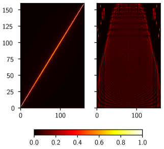
Figure 5: Matrix elements $|U_{ik}|$ (see Eq. (18)) in the star geometry (left) and in the chain geometry (right) for $N=159$ for the semi-circular bath as in Fig. 3. While the non-zero entries in star geometry are strongly concentrated around the diagonal, $U_{ik}$ in the chain geometry has $\sim N^{2}$ relevant non-zero elements. Note that for the star geometry, the terms $U_{ik}=V_{k}$ for $i=I$ (see Eq. (22)) are located at the bottom of the plot, but are barely visible.

We can understand the observed behavior for TEBD in both geometries by examining the matrix elements of the Trotter error terms in Eq. (16) and Eq. (10). We start with the many-body ground state for $U=0$, i.e., the filled Fermi-sea (FS):

$$\ket{\psi_{0}}=\prod_{k\in FS}c^{\dagger}_{k}\ket{0},$$ (19)

where $k$ labels the eigenstates of the hopping matrix $T_{ij}$ (Eq. (18)). As we have seen above, the leading errors of the Trotter decompositions correspond to hopping terms from one site to another. The error for the Green’s function is then given by the matrix element of Eq. (15) (star) and Eq. (10) (chain) with the state $c_{I}^{\dagger}\ket{\psi_{0}}$. The exact time evolution operator for $U=0$ is simply $U(t)=\prod_{k}e^{-iE_{k}t}n_{k}$, i.e., a time dependent phase factor for each occupied $k$. To find the magnitude and the number of terms contributing to the total error it hence suffices to evaluate (using the exact ground state (the Fermi-sea) for $\bra{\psi_{0}}$):

$$\bra{\psi_{0}}c_{I}c^{\dagger}_{i}c_{j}c_{I}^{\dagger}\ket{\psi_{0}}.$$ (20)

The indices $i$ and $j$ are determined by the various hopping terms appearing in Eq. (15) and Eq. (10). In $k$-space, we find:

$$\bra{\psi_{0}}c_{I}c^{\dagger}_{i}c_{j}c_{I}^{\dagger}\ket{\psi_{0}}= \sum_{k>FS}U^{\dagger}_{kI}U_{Ik}\sum_{k^{\prime}\in FS}U^{\dagger}_{k^{\prime}i}U_{jk^{\prime}}$$ (21)

$$+ \sum_{k,k^{\prime}>FS}U^{\dagger}_{Ik^{\prime}}U_{kI}U^{\dagger}_{ki}U_{jk^{\prime}},$$

where $U_{ik}$ are the matrix elements of the unitary transformation in Eq. (18), and the index value $I$ again denotes the impurity. Note that this expression is valid for both the star- and the chain geometry. Differences between them are encoded in the different unitary transformations $U_{ik}$ diagonalizing the hopping matrix $T_{ij}$. In star geometry, the bath states with energy $\epsilon_{k}$ are already very close to the eigenstates of $T_{ij}$. This implies that most entries in $U_{ik}$ are nearly zero, except for a few values around $i=k$. Indeed, as Fig. 5 (left plot) demonstrates, $U_{ik}$ in star geometry has relevant non-zero entries only around the diagonal. This means that in star geometry there are only $\sim N$ relevant terms in the matrix products in Eq. 21. In other words, not all terms of $\mathcal{C}_{\text{star}}$ contribute and we expect an error independent of system size for the leading order $({\Delta t})^{3}$. To make this point more clear, let us look at the case where only the diagonal of $U_{ik}$ contributes:

$$U_{ik}^{\text{star}}\approx\left\{\begin{array}[]{lr}\delta_{i,k}\text{, for }i\neq I\\ \sim V_{k}\text{, for }i=I\end{array}\right.$$ (22)

We note that the approximation $U_{Ik}\sim V_{k}$ is in good agreement with the true form of $U_{ik}$. Because of Eq. (22), $\mathcal{C}_{\text{star}}$ does not scale with system size anymore, since $\delta_{ik}$ always removes at least one summation. This remains true, when $U_{ik}^{\text{star}}$ contains a finite width band of relevant values instead of just the diagonal. For the chain geometry on the other hand $U_{ik}$ is a full matrix with $\sim N^{2}$ entries of similar size, as shown in Fig. 5 (right plot). Therefore, no such simplification occurs and the error should indeed scale linearly with $N$.
For TDVP, such arguments do not hold, since its error is independent of the bath geometry used. The evaluation of the corresponding commutators is far from trivial and we hence leave this point open for future studies.

V.2 Finite $U$

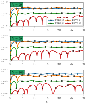
Figure 6: Absolute difference of $\Re G^{>}_{\text{ref}}(t)$ between high precision reference calculations and calculations with lower precision for various bath sizes and $U=1$. The bath was obtained from a semi-circular spectral function $-\frac{1}{\pi}\mathcal{I}\Delta(\omega)=\frac{1}{2\pi}\sqrt{1-\omega^{2}}$.
Because of the results at $U=0$, we chose TEBD for the star geometry and TDVP for the chain geometry for the reference calculations. These used a truncated weight of $10^{-14}$ ($10^{-13}$) and a Trotter time-step ${\Delta t}=0.005$ (${\Delta t}=0.005$) for TEBD (TDVP) respectively. Parameters for the other calculations were ${\Delta t}=0.05$ and truncated weight $10^{-12}$, the same as in Fig.3. The bond dimensions of the MPS were not restricted to a maximal value.

In Fig. 6 we show a comparison similar to Fig. 3, now for $U=1$. Since in the interacting case we do not have access to the exact solution, we compare to reference calculations with very high precision done separately for each bath size (see Fig. 6 for details). Overall, we find that the errors of lower precision calculations in Fig. 6 are almost identical to the ones obtained in the non-interacting case. In particular, we again find that only the error of TEBD-C scales appreciably with system size (see Fig. 4).
The necessary bond dimension on the other hand changes drastically. Using the semi-circular bath spectral function, the maximal value was $m_{\text{star}}=364$ $(128)$ compared to $m_{\text{chain}}=260$ $(214)$ for TEBD (TDVP) respectively.
So far, we only compared the error for a given set of parameters (i.e., truncation $t_{w}$ and time step $\Delta t$). The actual quantity of interest is the computation time for given accuracy (or vice versa). Although all algorithms scale$~{}\sim m^{3}$, their computation times are very different and comparisons are not straightforward for several reasons.

First, in star geometry the bond dimensions is strongly peaked around the center bath site, whereas in chain geometry it is more flat. Therefore, the maximal bond dimension is not a good indicator of actual computation times. Second, a single TDVP step is generally much more expensive than a TEBD step. For example, in the calculations shown in Fig. 6, TEBD-S is faster than TDVP-S although the maximal bond dimension is larger by a factor of three in TEBD-S. Third, TDVP generally allows for much larger time steps $\Delta t$ for a give accuracy.

Additionally, the advantage of the different geometries will likely depend on the actual bath parameters. For DMFT, most of the calculations are performed close to the self consistent point. We therefore studied the computation times necessary to reach a prescribed precision at the self consistent point of the Bethe lattice at $U=2$ ($U=4$ in the units of Ref. Wolf et al., 2014) for a time evolution up to $t=15$.

Alg.	$\Delta t$	$t_{w}$	Error ($10^{-4}$)	Wall time (s)
TEBD-C	$0.005$	$10^{-10}$	$2.5$	2370
TDVP-S	$0.005$	$10^{-12}$	$1.0$	4434
TEBD-S	0.1	$10^{-9}$	1.7	35
TEBD-S	0.01	$10^{-11}$	0.14	384
TEBD-S	0.01	$10^{-13}$	0.01	1655
TDVP-C	0.5	$10^{-8}$	2.6	457
TDVP-C	0.1	$10^{-10}$	0.2	1856
TDVP-C	0.05	$10^{-12}$	0.02	7130

Table 1: Comparison of computation times for the $U=2$ Bethe lattice self consistent bath. We chose example parameters for the time step $\Delta t$ and the truncated weight $t_{w}$ to approximately obtain errors of different orders of magnitude $10^{-4}$ to $10^{-6}$. We used the largest time step out of $\{0.005,0.01,0.05,0.1,0.5\}$ for which this error can be achieved with low enough truncated weights and then used the largest truncated weight at this time step with a similar error. For TEBD-C and TDVP-S only an error of about $10^{-4}$ was possible with the parameters studied. Reference calculations were again performed with TDVP-C in chain-geometry ($\Delta t=0.005$, $t_{w}=10^{-13}$) and TEBD-S in star geometry ($\Delta t=0.005$, $t_{w}=10^{-14}$). Wall times are reported for a Intel(R) Core(TM) i7-7740X CPU using a single thread and for a single calculation of $G^{>}(t)$ up to $t=15$ including DMRG for $N=59$.

Results are shown in Tab. 1. The two algorithms with large errors in Figs. 3 and 6, TEBD-C and TDVP-S are not able to obtain errors smaller than approximately $10^{-4}$ for the parameters studied and are comparable in computation time (TDVP-S has about half the error of TEBD-C but double the computation time). Additionally, they are slow compared to the other two approaches confirming behavior seen in Fig. 3 and Fig. 6.
Let us now compare the two favorable algorithms, TDVP-C and TEBD-S. While from Fig. 3 and Fig. 6 on would expect TDVP-C to be the better algorithm, Tab. 1 clearly shows that TEBD in star geometry is actually superior to TDVP-C. Its computation times are lower by about a factor of $5$ or more for the same error. Conversely, for similar computation times, the error of TEBD-S is about one order of magnitude smaller than TDVP-C. This shows that TEBD in star geometry is the best approach to calculate impurity Green’s functions and should also be considered the time evolution algorithm of choice for general non-equilibrium impurity problems as clever arrangement of sites allows time evolutions to be performed up to surprisingly long times Rams and Zwolak (2019).

VI Conclusions

We compared tensor network time evolution algorithms for Anderson Impurity Models for different bath representations. Specifically, we used TEBD and TDVP for the star- as well as the chain-geometry. TDVP is readily applicable for the long-range hybridizations present in the star geometry. For TEBD this is not the case and we explained in some detail the adapted TEBD approach using swap-gates first published in Ref. Bauernfeind et al., 2017. Its major advantage is that each actual time evolution gate can be combined with a swap gate, involving no additional computational cost and thus preserving the simplicity of TEBD. For TEBD, we additionally performed an analytic calculation of the leading order of the error due to the Suzuki-Trotter decomposition in both the star- and chain-geometry. This and the approximations of TDVP led us to expect that the error in the Green’s function should be proportional to the system size $N$ in all four cases. Surprisingly, we found that only TEBD in chain-geometry shows this behavior. We were able to find an analytical explanation of the better scaling of TEBD in star geometry from the fact that the bath states in star geometry are already a good approximation to the single particle eigenbasis and therefore, most error terms do not contribute. For DMFT calculations, such a favorable scaling with system size is especially important, since one has to make sure to use large bath sizes $N$ to represent the bath hybridization well enough to reach the correct self-consistent point.
Regarding the magnitude of the error, it is important to use the best combination of time evolution algorithm and bath representation. TDVP is more precise in the chain geometry likely due to the absence of projection error in the chain geometry. For TEBD it turned out to be vice versa, i.e., star geometry has a lower error. With given set of parameters (time step $\Delta t$ and truncated weight $t_{w}$) TDVP in chain geometry has the lowest error. On the other hand, the actual quantity of interest is the computation time for a given maximal error. With this metric, we found that TEBD in star geometry is the most favorable algorithm, faster than TDVP in chain geometry by about a factor of $5$ or more. Combined with its general simplicity and stability, this makes TEBD in star geometry at present the best approach to solve impurity problems using real-time evolution.

References

- Metzner and Vollhardt (1989) W. Metzner and D. Vollhardt, Phys. Rev. Lett. 62, 324 (1989).
- Georges and Kotliar (1992) A. Georges and G. Kotliar, Phys. Rev. B 45, 6479 (1992).
- Georges et al. (1996) A. Georges, G. Kotliar, W. Krauth, and M. J. Rozenberg, Rev. Mod. Phys. 68, 13 (1996).
- Anderson (1961) P. W. Anderson, Phys. Rev. 124, 41 (1961).
- Werner et al. (2006) P. Werner, A. Comanac, L. de’ Medici, M. Troyer, and A. J. Millis, Phys. Rev. Lett. 97, 076405 (2006).
- Gull et al. (2011) E. Gull, A. J. Millis, A. I. Lichtenstein, A. N. Rubtsov, M. Troyer, and P. Werner, Rev. Mod. Phys. 83, 349 (2011).
- Wilson (1975) K. G. Wilson, Rev. Mod. Phys. 47, 773 (1975).
- Bulla et al. (2008) R. Bulla, T. A. Costi, and T. Pruschke, Rev. Mod. Phys. 80, 395 (2008).
- Lu et al. (2014) Y. Lu, M. Höppner, O. Gunnarsson, and M. W. Haverkort, Phys. Rev. B 90, 085102 (2014).
- Zgid et al. (2012) D. Zgid, E. Gull, and G. K. L. Chan, Phys. Rev. B 86, 165128 (2012).
- Mejuto Zaera et al. (2017) C. Mejuto Zaera, N. M. Tubman, and K. B. Whaley, arXiv e-prints (2017), arXiv:1711.04771 [cond-mat.str-el] .
- White (1992) S. R. White, Phys. Rev. Lett. 69, 2863 (1992).
- Schollwöck (2011) U. Schollwöck, Ann. Phys. 326, 96 (2011).
- Bauernfeind et al. (2017) D. Bauernfeind, M. Zingl, R. Triebl, M. Aichhorn, and H. G. Evertz, Phys. Rev. X 7, 031013 (2017).
- Bauernfeind et al. (2018) D. Bauernfeind, R. Triebl, M. Zingl, M. Aichhorn, and H. G. Evertz, Phys. Rev. B 97, 115156 (2018).
- Paeckel et al. (2019) S. Paeckel, T. Köhler, A. Swoboda, S. R. Manmana, U. Schollwöck, and C. Hubig, arXiv e-prints (2019), arXiv:1901.05824 [cond-mat.str-el] .
- Haegeman et al. (2011) J. Haegeman, J. I. Cirac, T. J. Osborne, I. Pižorn, H. Verschelde, and F. Verstraete, Phys. Rev. Lett. 107, 070601 (2011).
- Haegeman et al. (2016) J. Haegeman, C. Lubich, I. Oseledets, B. Vandereycken, and F. Verstraete, Phys. Rev. B 94, 165116 (2016).
- Wolf et al. (2014) F. A. Wolf, I. P. McCulloch, and U. Schollwöck, Phys. Rev. B 90, 235131 (2014).
- Vidal (2003) G. Vidal, Phys. Rev. Lett. 91, 147902 (2003).
- Vidal (2004) G. Vidal, Phys. Rev. Lett. 93, 040502 (2004).
- Daley et al. (2004) A. J. Daley, C. Kollath, U. Schollwöck, and G. Vidal, Journal of Statistical Mechanics: Theory and Experiment 2004, P04005 (2004).
- Saberi et al. (2008) H. Saberi, A. Weichselbaum, and J. von Delft, Phys. Rev. B 78, 035124 (2008).
- Ganahl et al. (2015) M. Ganahl, M. Aichhorn, H. G. Evertz, P. Thunström, K. Held, and F. Verstraete, Phys. Rev. B 92, 155132 (2015).
- Kennes and Karrasch (2016) D. Kennes and C. Karrasch, Computer Physics Communications 200, 37 (2016).
- Suzuki (1990) M. Suzuki, Physics Letters A 146, 319 (1990).
- Note (1) For example a semi-circular bath spectral function can be represented by for all sites. Note that we use the Lanzcos tri-diagonalization instead.
- Bauernfeind (2018) D. Bauernfeind, Fork Tensor Product States: Efficient Multi-Orbital Impurity Solver for Dynamical Mean Field Theory, Ph.D. thesis, Graz University of Technology (2018).
- Orús (2014) R. Orús, The European Physical Journal B 87, 280 (2014).
- Verstraete et al. (2009) F. Verstraete, J. I. Cirac, and J. I. Latorre, Phys. Rev. A 79, 032316 (2009).
- Rams and Zwolak (2019) M. M. Rams and M. Zwolak, arXiv e-prints (2019), arXiv:1904.12793 [cond-mat.str-el] .