IFJPAN-IV-2019-5

QED Exponentiation for quasi-stable charged particles: the $e^{-}e^{+}\to W^{-}W^{+}$ process^†

S. Jadach^a, W. Płaczek^b and M. Skrzypek^a
a Institute of Nuclear Physics, Polish Academy of Sciences,
ul. Radzikowskiego 152, 31-342 Kraków, Poland
^b Institute of Applied Computer Science, Jagiellonian University,
ul. Łojasiewicza 11, 30-348 Kraków, Poland

All real and virtual infrared singularities in the standard analysis of the perturbative Quantum Electrodynamics (like that of Yennie–Frautschi–Suura) are associated with photon emissions from the external legs in the scattering process. External particles are stable, with the zero decay width. Such singularities are well understood at any perturbative order and are resummed. The case of production and decay of the semi-stable neutral particles, like the $Z$-boson or the $\tau$-lepton, with the narrow decay width, $\Gamma/M\ll 1$, is also well understood at any perturbative order and soft-photon resummation can be done. For an absent or loose upper cut-off on the total photon energy $\omega$, production and decay processes of the semi-stable (neutral) particles decouple approximately and can be considered quasi-independently. In particular, the soft-photon resummation can be done separately for the production and the decay, treating a semi-stable (neutral) particle as stable. QED interference contributions between the production and decay stages are suppressed by the $\Gamma/M$ factor. If experimental precision $\omega$ is comparable with or better than $\Gamma/M$, these interferences have to be included. In the case of $\omega\ll\Gamma$ decoupling of production and decay does not work any more and the role of semi-stable particles is reduced to the same role as that of other internal off-shell particles. So far, consistent treatment of the soft photon resummation for semi-stable charged particles like the $W^{\pm}$ bosons is not available in the literature, and the aim of this work is to present a solution to this problem. Generally, this should be feasible because the underlying physics is the same as in the case of neutral semi-stable resonances – in the limit of $\Gamma/M\ll 1$ the production and decay processes for charged particles also necessarily decouple due to long lifetime of intermediate particles. Technical problems to be solved in this work are related to the fact that semi-stable charged particle are able to emit photons. Practical importance of the presented technique to the $e^{+}e^{-}\to W^{+}W^{-}$ process at the Future electron–positron Circular Collider (FCC-ee) is underlined.

• This work is partly supported by the Polish National Science Center grant 2016/23/B/ST2/03927 and the CERN FCC Design Study Programme.

IFJPAN-IV-2019-5

1 Introduction

The Standard Model Electroweak (EW) Field Theory was confirmed as the correct physics theory of electromagnetic and weak interactions between elementary particles by precision measurements of the LEP experiments [1, 2]. The LEP data were precise enough to test all important dynamical properties of the EW theory, such as quantum loop effects, consequences of the renormalisation, multiple photon emission, etc. In particular, EW gauge cancellations and quantum loop effects were verified experimentally at LEP in the $e^{+}e^{-}\to W^{+}W^{-}$ process at the precision tag for the total cross section at the level of $0.3$–$05\%$. The mass of the $W$-boson was also measured directly with the precision of $33\,$MeV.

The electron-positron Future Circular Collider (FCC-ee) [3, 4], considered as the future project at CERN, will be able to produce the number of $W$-boson pairs by a factor of $10^{3}$ higher than at LEP. This will serve to determine total $WW$ cross section, the mass and width of $W$ with the unprecedented precision and search for any anomalous phenomena beyond the Standard Model (SM) of the EW and strong interactions. Obviously, analysing FCC-ee data will also require new SM perturbative calculations for the $e^{+}e^{-}\to W^{+}W^{-}$ process, much more precise than these available at the LEP era [5, 6] The precision tag expected in FCC-ee experiments is at the level of about $0.01\%$, a factor of $10$ better than at LEP. This will require to go beyond the state of the art of the LEP era in the calculations of the SM predictions for the $e^{+}e^{-}\to W^{+}W^{-}$ or $e^{+}e^{-}\to 4f$ processes.

For general discussion of the theoretical issues in the $W$-pair production process the reader should consult the reviews of refs. [7, 8]. In particular, the delicate question of the EW gauge invariance for the Dyson summation leading to imaginary part of the $W$ and $Z$ propagators is covered there.

Here we shall focus on the important QED part of the EW/SM perturbative corrections to the $W$-pair production process. More precisely, on this part of the QED corrections which is related to soft and collinear (SC) singularities for real and virtual photon emissions on the external legs. According to the accumulated knowledge on the SC photonic contribution, it is quite clear that they factorise either at the amplitude level, or for the differential distributions and can be calculated separately to a much higher order than the remaining genuine EW corrections. This is very convenient, because SC contributions are much bigger numerically than genuine EW corrections, simpler to calculate, and can be resummed to the infinite order. Once separation of the QED and EW parts is established, resummation of some higher-order contributions in each of these two classes can be done independently. The important nontrivial final step is then merging/matching them in the final results.

There is little doubt that the factorisation and resummation of the QED soft/collinear corrections is the key to the success in the high-precision calculations of the SM predictions for the $W$-pair production process at FCC-ee.

There are four classes of QED corrections to the $W$-pair production and decay process: initial-state corrections (ISR), final-state corrections (FSR) in the decays of two $W^{\pm}$, final-state Coulomb corrections (FSC) and the so-called non-factorisable interferences (NFI) between the production and the decays (IFI) and between two $W^{\pm}$ decays (FFI). The IFI corrections are suppressed due to relatively long lifetime of $W$’s and FFI due to large space separation. The effects due to ISR are numerically the biggest but also easier to control, while the FSR effects can be also quite sizeable for typical experimental cut-offs.

The IFI and FFI interferences are small, suppressed by the factor $\Gamma_{W}/M_{W}$ away from the $WW$-production threshold, strongly cut-off dependent and algebraically most complicated. At LEP they could be neglected but for the FCC-ee precision they have to be handled with great care!

The relative narrowness of the $W$ boson resonance not only causes suppression of the QED interferences, but also provides for the expansion in terms of $\Gamma_{W}/M_{W}\sim$ ${\cal O}(\alpha)$ of the matrix element of the $e^{+}e^{-}\to 4f$ process into the numerically biggest and physically most interesting double-resonant $e^{+}e^{-}\to W^{+}W^{-}$ part, and less important single-resonant and non-resonant background parts. In the following we shall refer to them as the double-pole (DP), single-pole (SP) and non-pole (NP) contributions, as it was common in the LEP-era literature.

The above pole expansion (POE) in the powers of $\Gamma_{W}/M_{W}$, disentangling the DP, SP and NP components at the scattering amplitude-level is very useful because it allows for each of these three components to calculate the genuine EW corrections at a different perturbative order and to perform resummation of the QED soft/collinear contributions at a different sophistication level. In the final stage of the calculation, the best way is to sum POE contributions coherently at the amplitudes level, before summing over spin and taking modulus squared, rather than for differential cross sections, thus avoiding proliferation of many interference terms.

At the time of LEP experiments, two solutions based on the pole expansion were worked out, in which the ${\cal O}(\alpha^{1})$ EW corrections were complete only for the DP component $e^{+}e^{-}\to W^{+}W^{-}$ of the $e^{+}e^{-}\to 4f$ process. One of them, nicknamed KandY [9, 10], was based on the combination of YFSWW3[11, 12] Monte Carlo (MC) for the $e^{+}e^{-}\to W^{+}W^{-}$ and $W^{\pm}$-decay processes with another MC program KORALW[17] for the remaining background. The multiphoton emission for ISR, including higher orders, was implemented using the soft-photon resummation inspired by the Yennie–Frautschi–Suura (YFS) work[18]. The QED FSR was added in $W$ decays using the PHOTOS program [19, 20]. Another POE-based solution was that of RACOONWW [21, 22], also with the complete EW ${\cal O}(\alpha^{1})$ corrections implemented only for the signal $e^{+}e^{-}\to W^{+}W^{-}$ process and not for the background part.

Implementation of QED corrections in RACOONWW was very different from that in KandY. On the one hand, RACOONWW was using exact matrix element for the entire $e^{+}e^{-}\to 4f\gamma$ process but it was lacking sophisticated soft photon resummation of the KandY. For more detailed comparison of the two approaches see the review of ref. [8] or more recent of ref.[23]. Both approaches were instrumental in the analysis of the LEP data for the $e^{+}e^{-}\to W^{+}W^{-}$ process [2], where the gauge cancellations and the quantum effects of the EW theory were tested experimentally for the first time.

Both approaches, KandY and RACOONWW, neglect terms of ${\cal O}(\alpha\Gamma_{W}/M_{W})$. The QED NFI interferences between $W$ production and decays were either neglected completely (KandY) or included in the soft-photon approximation (RACOONWW) without resummation. The overall precision of these calculations was about $0.3$–$0.5\%$. The FCC-ee experiments will require new calculations with the precision tag below $0.1\%$, thus adding missing $\alpha\Gamma_{W}/M_{W}$ corrections, ${\cal O}(\alpha^{2})$ electroweak corrections to the DP component, a more advanced QED factorisation/resummation scheme, subleading QED ${\cal O}(\alpha^{2})$ corrections and more will be needed [5, 6]. In particular, inclusion the QED NFI corrections in the fully exclusive way, taking into account the $\Gamma_{W}/M_{W}$ suppression, will be necessary.

The aim of the present work is to work out a new methodology of the soft photon resummation including NFI corrections for charged unstable particles, similarly as it was done for the production and decay of the narrow neutral $Z$-boson in the process $e^{+}e^{-}\to f\bar{f}+n\gamma$ with a built-in $\Gamma_{Z}/M_{Z}$ suppression for the QED initial-final interferences (IFI) at any perturbative order [24, 25]. This method was already tested for the $Z$ resonance in the Monte Carlo event generator KKMC[24]. Its matrix element is built according to the so-called coherent exclusive exponentiation (CEEX) scheme, in which factorisation of the infrared (IR) divergences is done entirely at the amplitude level (before squaring and spin-summing). The older version of the exclusive exponentiation (EEX) of refs.[26, 27] was done at the level of differential distributions for the same $e^{+}e^{-}\to f\bar{f}+n\gamma$ process and features multiphoton resummation of ISR and FSR. Both approaches, CEEX and EEX, are inspired by the pioneering work of Yennie–Frautschi–Suura [18].

In the present work we shall generalise the CEEX scheme to the case of any number of narrow charged intermediate resonances, like the $W$-boson – the scheme is however quite general and applies to any charged resonance of any spin. The new CEEX scheme provides exclusive (unintegrated) description for multiple real photons of any energy, for $E_{\gamma}\sim\Gamma_{W}$, $E_{\gamma}\ll\Gamma_{W}$ and $E_{\gamma}\sim\sqrt{s}$, with all QED interferences between production and decays properly accounted for. Multiple real and virtual photon emission from all external stable particles and the intermediate semi-stable charged resonance will be described correctly in the soft photon limit and summed up to the infinite order. As in the case of CEEX of refs. [24, 25], its present extension will provide for a well-defined methodology of incorporating non-soft contributions (including the genuine EW corrections) calculated up to a finite perturbative order into multiphoton amplitudes of the soft-photon resummation scheme. In particular, sizeable but easier to calculate QED non-soft collinear contributions can also be included easily up to an arbitrarily high order.

The consistent resummation of the apparently IR-divergent contribution due to photon emissions from the semi-stable intermediate charged particle (narrow resonances) in the perturbative expansion is a non-trivial issue. Let us first consider $\Gamma\to 0$ limit. The best illustrative example is that of the $\tau^{\pm}$-pair production and decay in the $e^{+}e^{-}$ annihilation where a time scale of the $\tau$-pair formation (production process) is shorter than the $\tau$ lifetime by at least a factor of $\Gamma_{\tau}/m_{\tau}\simeq 3\cdot 10^{-12}$, hence photons emitted in these two stages get completely decoupled and the QED effects in the production and the decay can be implemented separately [28, 29, 24].

The situation in the $W$-pair production is similar but the suppression factor $\Gamma_{W}/M_{W}\simeq 0.026$ is not that small. The QED interferences are therefore expected to be of the order of $\alpha\Gamma_{W}/M_{W}\simeq 2\cdot 10^{-4}$. In LEP experiment this size could be neglected, but for the FCC-ee precision, effects of this size have to be calculated and taken into account. Moreover, such interferences depend on kinematical cut-offs – from the experience with the $Z$-boson case we know that they may grow by a factor of $2$–$5$ even for relatively mild cut-offs on photon energies. Also, in the case when photon energy resolution $\omega$ of the detector approaches $2\,$GeV, which is the case for FCC-ee detectors, photon emission from FSR in the production process and from $W$ decays cannot be separated and treated in the soft photon approximation, consequently the off-shell $W$’s have to be treated the same way as other internal exchanges in the $e^{+}e^{-}\to 4f$ process.

Our aim is to construct a variant of CEEX spin amplitudes in which we profit as much as possible from the smallness of $\Gamma_{W}/M_{W}$ and the classic YFS soft-photon limit for the entire $e^{+}e^{-}\to 4f$ process is correctly reproduced for $\omega\ll\Gamma_{W}$. The basic technical problem will be that if we want to treat $W$’s as stable particles in the $W$-pair production process with the zero width, then amplitudes of photon emission from $W$ must be IR-singular, while for the semi-stable $W$’s they are not (the $W$ width acts as a IR regulator). Our aim is to reconcile these two contradictory situations in a single algebraic framework.

In the YFSWW3 program, photon emission in the $e^{+}e^{-}\to W^{+}W^{-}\to 4f$ process was treated in a similar way as in the above $\tau$-pair production and decay, except that $W$ invariant masses were not fixed but modelled according to the Breit–Wigner shape. The QED matrix element in YFSWW3 for $e^{+}e^{-}\to W^{+}W^{-}$ with the soft photon resummation is of the EEX type, including ISR, FSR and IFI. Decays of $W^{\pm}$s are supplemented with additional photons using PHOTOS. However, it could be easily replaced with the multiphoton MC implementation of the EEX of the WINHAC program [30]. Once EEX implementation is available in the $W$-pair process for the production and decays, the new CEEX matrix element developed in the present work can be introduced using an additional multiplicative MC weight, without any change in the underlying MC program. The above would be the solution for the resummed QED corrections of the DP part of the $e^{+}e^{-}\to 4f$ process. The ${\cal O}(\alpha^{1})$ and ${\cal O}(\alpha^{2})$ genuine EW corrections can be added in the on-shell approximation within the CEEX matrix element in the similar way as it was done for the $e^{+}e^{-}\to 2f$ process in refs. [24, 25]. So far only ${\cal O}(\alpha^{1})$ EW corrections are available. In order to exploit fully FCC-ee data, the ${\cal O}(\alpha^{2})$ EW corrections will be needed. As pointed out in ref. [5], the clear and clean separation of the QED and the genuine EW correction at any perturbative order is a useful built-in feature of the CEEX factorisation/resummation scheme.

The single-pole group of diagrams of the $e^{+}e^{-}\to 4f$ process process is separated at the amplitude level in the CEEX scheme. It would be enough to include the genuine EW corrections to the SP part at ${\cal O}(\alpha^{1})$. They are in principle known, because they are part of the ${\cal O}(\alpha^{1})$ corrections to $e^{+}e^{-}\to 4f$ process in refs. [31, 32], although it may be not simple to disentangle them from the rest of the existing calculations. For the non-pole part of the $e^{+}e^{-}\to 4f$ process it would probably be enough to take it at the tree-level as far as the genuine EW corrections are concerned and take care of the QED corrections only, either in the CEEX or EEX scheme.

In this work, the CEEX scheme will be defined only for the DP part leaving the easier SP and NP variants for the future development. On the other hand, we shall also discuss in a more detail the explicit algebraic relation between the CEEX scheme and the EEX scheme of the YFSWW3. This will provide better understanding of the theoretical foundation of the existing EEX scheme of the YFSWW3. The main result of this work is, however, that it provides an important building block for the future high-precision calculations for the $W$ pair production process, and also for any other process with narrow charged resonances.

Close to the $WW$ threshold, where the $W$ mass is planned in the FCC-ee experiment to be measured with the $\leq 0.5\,$MeV precision (using the total cross section [3, 4]), the problem is that the pole expansion for the non-QED part of the scattering matrix element is not efficient any more. The partial suppression of the QED IFI and FFI corrections will still work close to threshold as long as resonant curves of $W$’s are not fully “distroyed” by the threshold cut-off. However, as shown in works based on the effective field theory (EFT) [33, 34], near the threshold one may exploit expansion in the Lorentz velocity $\beta=\sqrt{s-4M_{W}^{2}}/2M_{W}\ll 1$ of the $W$’s in order to reduce substantially a number of diagrams, such that higher-order EW and QED corrections are again within the reach of practical evaluations. This kind of expansion should be exploited in the standard diagrammatic approach as well.

Summarising, a combination of the pole expansion and of the QED exclusive exponentiation has already proven to be an economical solution for precision calculations of the SM prediction for the $W$-pair production process at LEP and is the best candidate for the further development in future electron-positron collider projects, especially for FCC-ee. The inclusion of the QED interferences between the $W$ production and decays, and of other missing corrections of the order of $\alpha\Gamma_{W}/M_{W}$ will require applying a more sophisticated soft/collinear photon factorisation and resummation scheme, combined with POE. We propose here a new solution based on the coherent exclusive exponentiation, CEEX, in which resummation of the infrared (IR) divergences is done entirely at the amplitude level. The interesting feature of this new scheme is that the $\Gamma_{W}/M_{W}$ suppression of the QED interferences between production and decay is a built in feature valid in any order and at any photon energy scale/resolution, all over the entire multiphoton phase space. The new scheme is similar to the CEEX scheme previously formulated and successfully applied to the case of the neutral intermediate resonances (the $Z$-boson).

One should not give up on the more traditional EEX schemes, however. We shall discuss briefly alternative solutions within the traditional EEX schemes (extensions of EEX of YFSWW3). We shall also examine approximations or simplification done in the transition from the CEEX to EEX schemes, and between various variants of them.

Concluding, this work provides an important building block for the future high-precision Standard Model calculations for the $W$-pair production process at the future $e^{+}e^{-}$ colliders.

The paper is organised as follows. In Section 2 we describe the pole expansion for the $W$-pair production process. Section 3 is devoted to a general discussion of various kinds of the exclusive QED exponentiation and a problem of photon emission from an intermediate semi-stable charged particle. In Section 4 we present details on the CEEX scheme for the process $e^{+}e^{-}\to 4f$ involving intermediate resonant $W$-bosons. Relations between the CEEX and EEX schemes are discussed in Section 5. Section 6 contains summary and outlook of our work. Finally, detailed derivations of factoring multiphoton radiation from an intermediate semi-stable charged particle, resummation of real-photon emissions and the virtual YFS form-factor for the pertinent process are given in Appendices A, B and C, respectively.

Shorter version of this work was reported in the conference materials of Ref. [35].

2 Pole expansion for $W$-pair production

As pointed out by R. Stuart [36], it is always possible to decompose the matrix element into a combination of Lorentz covariant tensors and Lorentz invariant functions. If unstable particles are involved in a process, one can then perform a Laurent expansion about complex poles corresponding to those unstable particles. However, only the Lorentz invariant functions (mathematically, analytic functions of complex variables) are subject to this expansion, while the Lorentz covariant and spinor structure of the matrix element should remain untouched. In the so-called leading-pole approximation (LPA) one retains only the leading terms in the above expansion, neglecting the rest of the Laurent series. As discussed in Ref. [36], the whole procedure does not violate gauge invariance of the matrix element. This is guaranteed by the fact that all terms in the pole expansion are independent of each other, e.g. in the case of two unstable particles, the doubly-resonant terms are independent of the singly-resonant and non-resonant ones, therefore there cannot be gauge cancellations between those terms. In Ref. [36], the process of $Z$-pair production and decay was presented as an example.

Here, we discuss the process of $W$-pair production and decay:

$$e^{-}(p_{1})+e^{+}(p_{2})\longrightarrow W^{-}(Q_{1})+W^{+}(Q_{2})\longrightarrow f_{1}(q_{1})+\bar{f}_{2}(q_{2})+f_{3}(q_{3})+\bar{f}_{4}(q_{4}),$$ (2.1)

where $W^{-}$ decays into $f_{1},\bar{f}_{2}$ and $W^{+}$ into $f_{3},\bar{f}_{4}$. At the lowest order, the minimum gauge invariant subset of Feynman diagrams needed for this process is the so-called CC11-class of graphs. It includes apart from doubly-resonant $WW$ graphs (the so-called CC03) also singly-resonant $W$ graphs. Below we discuss how to apply the pole expansion this process.

Since we are interested only in LPA (a double-pole approximation in this case) we start from extracting a part of the full matrix element that can give rise to doubly-resonant contributions (the rest will drop in LPA anyway). It can be written as follows:

$${\cal M} = \sum_{i}\left[\bar{v}_{e}(p_{2})T^{i}_{\mu\nu}u_{e}(p_{1})\right]M_{i}(s,t,s_{1},s_{2})$$ (2.2)

$$\times D_{W}^{-1}(s_{2})\left[\bar{u}_{f_{3}}(q_{3})\gamma^{\mu}V_{Wf}(s_{2})\omega_{-}v_{f_{4}}(q_{4})\right]$$

$$\times D_{W}^{-1}(s_{1})\left[\bar{u}_{f_{1}}(q_{1})\gamma^{\nu}V_{Wf}(s_{1})\omega_{-}v_{f_{1}}(q_{1})\right]\;,$$

where

$$D_{W}(s)=s-M_{W}^{2}+\Pi_{W}(s)$$ (2.3)

is a Dyson-resumed $W$ propagator with $\Pi_{W}(s)$ being the $W$ self-energy correction. In the above we have used the following notation:

$$\omega_{-}=\frac{1}{2}(1-\gamma_{5}),$$

$$s_{1}=Q_{1}^{2},\;s_{2}=Q_{2}^{2},$$ (2.4)

$$Q_{1}=q_{1}+q_{2},\;Q_{2}=q_{3}+q_{4}.$$

$T^{i}_{\mu\nu}$ are the Lorentz covariant tensors spanning the tensor structure of the matrix element, while $M_{i},\,\Pi_{W},\,V_{Wf}$ are Lorentz scalars that are analytic functions of independent Lorentz invariants of the process. These functions then undergo the Laurent expansion about the complex poles corresponding to a finite-range propagation of two $W$’s. Keeping only the leading terms in the above expansion, we end up with the LPA matrix element [10, 37]

$${\cal M}_{\rm LPA} = \sum_{i}\left[\bar{v}_{e}(p_{2})T^{i}_{\mu\nu}u_{e}(p_{1})\right]M_{i}(s,t,s_{p},s_{p})$$ (2.5)

$$\times\frac{F_{W}(s_{p})}{s_{2}-s_{p}}\left[\bar{u}_{f_{3}}(q_{3})\gamma^{\mu}V_{Wf}(s_{p})\omega_{-}v_{f_{4}}(q_{4})\right]$$

$$\times\frac{F_{W}(s_{p})}{s_{1}-s_{p}}\left[\bar{u}_{f_{1}}(q_{1})\gamma^{\nu}V_{Wf}(s_{p})\omega_{-}v_{f_{1}}(q_{1})\right]\;,$$

where the pole position $s_{p}$ is a solution to the equation

$$s-M_{W}^{2}+\Pi_{W}(s)=0,\quad F_{W}(s_{p})=[1+\Pi^{{}^{\prime}}_{W}(s_{p})]^{-1}.$$ (2.6)

At the lowest order the Lorentz tensors read

$$T_{\mu\nu}^{1,2} = \gamma^{\lambda}\Gamma_{\lambda\mu\nu}(Q,Q_{1},Q_{2}),$$ (2.7)

$$T_{\mu\nu}^{3} = \gamma_{\mu}(\not\!p_{2}-\not\!Q_{2})\gamma_{\nu},$$ (2.8)

and the Lorentz scalars are

$$M_{1} = e^{2}\frac{1}{s},$$ (2.9)

$$M_{2} = -e^{2}\frac{s_{W}}{c_{W}}[v_{e}-a_{e}\gamma_{5}]\frac{1}{s-M_{Z}^{2}+iM_{Z}\Gamma_{Z}},$$ (2.10)

$$M_{3} = \frac{e^{2}}{s_{W}^{2}}\frac{1}{t},$$ (2.11)

$$V_{Wf} = \frac{eU_{ij}\sqrt{N_{c}}}{2s_{W}^{2}},$$ (2.12)

where $Q=p_{1}+p_{2},\;s=Q^{2},\;t=(p_{2}-Q_{2})^{2}$, $U_{ij}$ is the CKM matrix element, $N_{c}$ is the QCD colour factor, $s_{W}=\sin\theta_{W}$, $c_{W}=\cos\theta_{W}$, $v_{e}$ and $a_{e}$ are the vector and axial couplings of a $Z$ boson to electrons, $\Gamma_{\lambda\mu\nu}$ is the $VWW$ coupling ($V=\gamma,Z$):

$$\Gamma_{\lambda\mu\nu}(Q,Q_{1},Q_{2})=(Q+Q_{1})_{\nu}g_{\lambda\mu}+(Q_{2}-Q_{1})_{\lambda}g_{\mu\nu}-(Q+Q_{2})_{\mu}g_{\nu\lambda}.$$ (2.13)

In the scalar function $M_{2}$ we have also applied LPA to the intermediate $Z$-boson. It is done in a similar way as for $W$’s. The $W$-pole position, up to ${\cal O}(\alpha^{2})$, is given by

$$s_{p}=M_{W}^{2}-iM_{W}\Gamma_{W}+{\cal O}(\alpha^{2}),$$ (2.14)

where $M_{W},\,\Gamma_{W}$ are the usual on-shell scheme $W$ mass and width, and $F_{W}=1$. One can easily check that at the lowest order this LPA matrix element has the same form as the CC03 matrix element calculated in ’t Hooft–Feynman gauge and in the constant $W$-width scheme. It was noticed in Ref. [38] that when the CC03 matrix element is calculated in the axial gauge also singly-resonant terms appear. This indicates that the singly-resonant graphs are needed to guarantee gauge invariance of the matrix element, i.e. that CC03 itself is not gauge-invariant, but one has to take at least CC11 for hadronic, CC10 for semi-leptonic and CC09 for leptonic final states. In the LPA approach described above it does not matter what gauge is used in the calculations. We start from the gauge-invariant matrix element and then apply the pole expansion. In the resulting LPA matrix element all non-double-pole terms drop out.

One of the complications that arises when going to higher orders is the fact that $W$’s are electrically charged and therefore radiate photons. When a real or virtual photon is emitted from the $W$ one has more than just two $W$ propagators in the matrix element and the question is how to apply the pole expansion in such a case. Here, however, one can exploit a partial-fraction decomposition of a product of two propagators, namely:

$$\frac{1}{Q^{2}-M^{2}}\frac{1}{{Q^{\prime}}^{2}-M^{2}}\equiv\frac{1}{2kQ^{\prime}+k^{2}}\frac{1}{{Q^{\prime}}^{2}-M^{2}}-\frac{1}{Q^{2}-M^{2}}\frac{1}{2kQ-k^{2}},$$ (2.15)

where $M^{2}=M^{2}_{W}+i\Gamma_{W}M_{W}$, $Q,\,Q^{\prime}=Q-k$ are the $W$ four-momenta before and after radiation of a photon of the four-momentum $k$, respectively. So, a product of two propagators can be replaced by a sum of single propagators multiplied by eikonal factors. This corresponds to splitting the photon radiation into the radiation in the $W$-production stage and the radiation in the $W$-decay stage. These two stages are separated by the finite-range $W$ propagation. The above decomposition can be applied both to the real and virtual photon emissions. In the case of the real photons the radiation amplitude splits into the sum of the amplitudes corresponding to photon emission in the $WW$-production and two $W$-decays. At the level of the cross section this results in the sum of contributions corresponding to the photon radiation at each stage of the process – the factorisable corrections, and the contributions corresponding to interferences between various stages – the non-factorisable corrections. Similarly, for the virtual corrections, the contributions with photons attached to the same stage give rise to the factorisable corrections, while the ones where photons interconnect different stages of the process contribute to the non-factorisable corrections. In this way all radiative corrections can be split in a gauge-invariant way into the factorisable and non-factorisable ones.

Since the non-factorisable corrections were negligible for the main LEP2 observables one could drop them and concentrate only on the factorisable ones. For factorisable corrections one can employ the existing calculation for the on-shell $WW$-production and the on-shell $W$-decay. Our aim is to treat the QED corrections according to the YFS exclusive exponentiation procedure and also apply the LPA, described above, in order to obtain the gauge-invariant formulation. How to do this? Extraction of infra-red (IR) contributions for both real and virtual photons can be done in a gauge-invariant way according to the YFS theory for each of the stages separately. These contributions are then sum up to infinite order and result in the so-called YFS form-factor. This means that the YFS form-factors and the IR real-photon $\tilde{S}$-factors involving $W$’s do not have to be taken on-pole but can be calculated like for stable particles. After having done this we can apply the pole expansion to the IR-residuals – the YFS $\bar{\beta}$-functions. We proceed in the way described at the beginning of this section and retain only the leading-pole (double-pole) terms. The ${\cal O}(\alpha)$ LPA matrix element for the real photon contribution reduces, similarly to the lowest order, to the form that can be obtained from the doubly-resonant Feynman graphs with single-photon emission in the ’t Hooft–Feynman gauge. The ${\cal O}(\alpha)$ virtual correction form-factors should, in principle, be evaluated on the complex pole. This would require an analytic continuation of the usual one-loop results to the second Riemann sheet (this may be a technical problem). However, for the aimed LPA accuracy, it is sufficient to use the approximation $s_{p}\simeq M_{W}^{2}$. This would correspond to neglecting terms of ${\cal O}(\frac{\alpha}{\pi}\frac{\Gamma_{W}}{M_{W}})$. More details about implementation of the ${\cal O}(\alpha)$ corrections in the $WW$-production process in the MC event generator YFSWW3 can be found in Ref. [11].

3 General discussion

In this section we collect discussion on various aspects of the photon radiation in the $W$ pair production process, in particular we discuss various exponentiation schemes preparing grounds for defining them explicitly in the following sections. We define more precisely our aims, discuss various constraints, introduce notation and terminology.

The fact that $W$’s are narrow resonances and behave like almost stable particles is of great practical importance for the evaluation of the radiative corrections, because it provides an additional small parameter $\Gamma_{W}/M_{W}$ which can be used as an expansion parameter, leading to reduction of the complexity of calculations of radiative corrections. As a result, the dominant double-resonant part of the process (3.3) can be well approximated as three independent processes: one production process and two decay processes. For the double resonant part it is possible to use simpler on-shell radiative corrections, while for the single-resonant part we may stay at the Born-level or use some crude leading-order (LO) approximations for the radiative corrections. Of course, we have to have at our disposal a method of splitting the Born amplitude and the amplitude with the radiative corrections into the double- and single-resonant parts, without breaking gauge invariance and other elementary principles. The pole expansion (POE) seems to be the best method available. Once POE is used for $W$-pair production process to isolate the double-pole (DP), single-pole (SP) and non-pole (NP) parts, photon emission from the intermediate unstable $W$’s has to be reorganised in a consistent way. In addition, it would be desirable to sum up photon emission from $W$’s to infinite order (exponentiate), for instance using one of EEX or CEEX schemes.

In the following we shall characterise various methods of the known soft photon resummation and then characterise problems related to soft-photon emission from charged semi-stable intermediate particles (resonances), like the $W$-bosons.

3.1 Various kinds of exclusive exponentiation

Resummation	Formalism	NFI interf.	Implementations	Order
No resonances
EEXB	[40, 18]	–	YFS1	${\cal O}(\alpha^{1})$
CEEXB	None	–	None	–
Neutral semi-stable intermediate particles
EEXR	[27]	No	YFS3, KORALZ	${\cal O}(\alpha^{3})$
CEEXR	[24, 25]	Yes	KKMC	${\cal O}(\alpha^{2})$
Charged semi-stable intermediate particles
EEXR	[11, 12]	No	YFSWW3	${\cal O}(\alpha^{3})$
CEEXR	This work	Yes	None	–

Table 1: The list of the exclusive soft photon resummation schemes and their implementations. The 2nd column indicates the primary reference for the formalism. Inclusion of the non-factorisable interference is marked in the 3rd column. Practical implementations in the MC codes are listed in the 4th column. The maximum (LO) order of the complete non-soft QED corrections is indicated in the last column.

Generally, there are two kinds of exclusive exponentiation schemes: (1) the older one, which we call EEX, in which isolation of IR singularities due to real photons is done for differential distributions (probabilities), as in the classic work of Yennie–Frautschi–Suura (YFS) [18], and (2) the newer one of refs. [41, 25, 24], referred to as CEEX, in which the same isolation of the real photon IR singularities is done for the amplitudes themselves, that is before squaring and spin-summing them. CEEX has a number of advantages over EEX. The price to pay is that it can be more complicated in the implementation and slower in the numerical evaluation.

Since we are interested mainly in the exclusive exponentiation for the processes with the narrow resonances, it is worth to note that, within EEX and CEEX families, there are two distinct subgroups of implementations which differ rather strongly in the treatment of the narrow resonances (or of sharp $t$-channel peaks). The key difference is in the treatment of the shift of the energy-momentum in the propagator of the resonance due to emission of the real or virtual photons. Let us, for the purpose of this work, call this effect a “recoil effect” or shortly a “recoil”.

Within the EEX family there is a baseline variant based on the original YFS work [18], in which the recoil is realised in an order-by-order way. Let us denote them with EEX_B. Examples of the EEX_B variants are: the unpublished MC code YFS1 described in ref. [40] and BHLUMI 1.x of ref. [42]. In EEX_B the recoil is absent completely at the level of ${\cal O}(\alpha^{0})_{\rm EEX}$. Then, it is gradually introduced in an order-by-order manner, through the so-called IR-finite $\bar{\beta}$-functions. For instance, in ${\cal O}(\alpha^{2})_{\rm EEX}$ the exact recoil in the differential distribution is realised due to two hard real photons – if there is a third “spectator” hard photon, then its contribution to resonance propagator is simply ignored. The problem is that, from the point of view of the strong variation of the resonance propagator, a photon with the energy of the order of the resonance width $\Gamma$ is already hard! This is why EEX_B can be disastrous for narrow resonances, where in order to realise the recoil, it would be mandatory to jump immediately to very high perturbative orders, otherwise the perturbative convergence for the QED corrections would be miserable. EEX_B can be a convenient and natural choice if there are no resonances at all.

In the second class of the EEX scenarios, the recoil in the resonance propagator (or sharp $t$-channel exchange) is a built-in feature of the scheme, which is present already in ${\cal O}(\alpha^{0})_{\rm CEEX}$. Let us call such a scheme EEX_R. It is realised for the first time in the YFS3 event generator [27] and later on included in the KORALZ [43], KKMC [24] programs and finally in the YFSWW3 program [11, 12]. The analogous scheme for a process dominated by the $t$-channel was implemented in the BHLUMI MC program [44, 45]. In EEX_R, the total energy-momentum in the resonance propagator (or $t$-channel exchange) includes the contribution from all real photons emitted prior to resonance formation ($t$-channel exchange). This means that for each photon we have to know whether it belongs to resonance production or decay process (ISR or FSR). This is possible because in this scenario one always neglects completely and irreversibly the QED interferences between the ISR and FSR. Neglecting these interferences may be not so harmful as compared to experimental precision, because they are suppressed by the $\Gamma/M$ factor. The EEX_R is obviously very well suited for narrow resonances, as long as we can afford neglecting ${\cal O}(\alpha\Gamma/M)$ interference corrections, and we do not attempt to examine experimentally spectra of photons with energies $E_{\gamma}\simeq\Gamma$.

In the CEEX family of exponentiations there are analogous two sub-classes: either the recoil is implemented in the infinite order (CEEX_R) or in the order-by-order manner (CEEX_B). One great advantage of CEEX is that, in the process with the resonant component and the non-resonant background, one may apply CEEX_R to the resonant part of the amplitude and CEEX_B to the background and add the two coherently afterwards.

Let us comment on the relation of the above schemes to the classic YFS work and the relation of EEX_R to other ones. All the above exponentiation schemes are inspired by the classic YFS work [18] in one way or another. However, it is in fact only the EEX_B scheme which was formulated explicitly in the original YFS work. CEEX is a non-trivial extension of the YFS exponentiation scheme, see ref. [25] for more discussion. So far, there is no implementation of the CEEX_B scheme, while more sophisticated CEEX_R is successfully implemented in KKMC [24] program for the neutral semi-stable $Z$ boson production and decay in the electron–positron annihilation and recently in the proton–proton collision [46].

The above inventory of all schemes of the exclusive QED exponentiations and their implementations are summarised in table 1.

Finally, let us note that there is another variant of the EEX_R scheme implemented in the BHWIDE program of ref. [47], featuring partial implementation of the QED NFI interferences for semi-stable neutral boson exchanges. It will be discussed in the following whether this kind of scheme could be extended to include the QED NFI interferences for the charged semi-stable $W$-boson.

3.2 Photons from intermediate semi-stable charged particle

Let us present an introductory discussion on the photon emission from the intermediate charged unstable $W$’s.

In order to better grasp physics of the photon emission from unstable charged particles, let us consider one more time the case of $e^{+}e^{-}\to\tau^{+}\tau^{-}+n\gamma,\;\;\tau^{\pm}\to X^{\pm}$ process. In this case, with $\Gamma_{\tau}/m_{\tau}=2.27\cdot 10^{-12}$, the production and decay processes are well separated in time due to this factor. For instance, the formation time of the $\tau$-pair at $\sqrt{s}=100\,$GeV is $\sim 10^{-24}\,$sec while the $\tau$ lifetime is much longer, $2.9\cdot 10^{-13}\,$sec. This is why the ISR photons emitted from initial beams have no chance to interfere with these of the $\tau$ decays. The FSR photons emitted from the outgoing ultrarelativistic $\tau$’s are quite copiously, because $\ln(s/m_{\tau}^{2})=8.06$, but still, the emissions of the FSR photons and photons in the decays are time-separated by the factor of $\Gamma_{\tau}/m_{\tau}=2.27\cdot 10^{-12}$. The suppression of the interferences between photon emission from two decays is even stronger, by the factor $\Gamma_{\tau}/\sqrt{s}\sim 10^{-14}$. Consequently, all practical calculation for QED effects in the $\tau$-pair production and decay process from the production threshold onwards were implemented in the Monte Carlo programs independently for the production and decay parts [28, 29, 24]. The $\tau$-leptons in the production process are treated in the perturbative/diagrammatic QED calculations and in the phase-space integration as stable particles with the fixed mass and the zero decay width. Photon emission from the unstable intermediate $\tau$’s is of course exponentiated – the same way in the decay parts. Can the above production-decay separation break down? Yes, if the energy resolution in the photon energy (a cut on photon energies) is smaller than the $\tau$ width, that is below $0.003\,$eV, which is experimentally unfeasible.

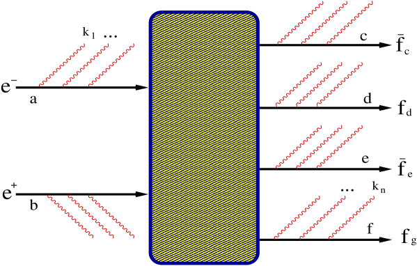
Figure 1: Kinematics of the four-fermion production process with multiple photons.

In order to see that the problem of the photon emission from the unstable intermediate $W$’s is not a completely trivial, let us recall a well-known elementary fact [18]: the emission of photons from the stable initial beams and four final fermions can be factorised into a product of the soft factors $\prod_{i}J_{6f}^{\mu_{i}}(k_{i})$ with the total electric current for all six external particles:

$$J_{6f}^{\mu}(k)=\hat{J}_{a}^{\mu}(k)+\hat{J}_{b}^{\mu}(k)+\hat{J}_{c}^{\mu}(k)+\hat{J}_{d}^{\mu}(k)+\hat{J}_{e}^{\mu}(k)+\hat{J}_{f}^{\mu}(k),$$ (3.1)

where

$$\hat{J}_{x}^{\mu}(k)=\theta_{x}Q_{x}\frac{2p_{x}^{\mu}\theta_{x}+k}{k^{2}+2k\cdot p_{x}\theta_{x}+i\varepsilon},$$ (3.2)

$p_{x}$ and $Q_{x}$ are the momentum and charge (in the units of positron charge) of the emitter particle $x$, and $\theta_{x}=+1,-1$ for the initial- and final-state particle, respectively. For the virtual photons there might be contractions among the pairs of the currents $J_{6f}^{\mu_{i}}(k_{i})$ and $J_{6f}^{\mu_{j}}(k_{j})$, see next sections for the explicit formulation. Fig. 1 provides a visual representation of the process of four-fermion production in electron–positron collisions. All possible contractions (loops) for the virtual photons are not explicitly marked there.

Strictly speaking, in the orthodox YFS scheme [18], the emissions from the intermediate $W$’s should not be included in the IR soft factors, because $W$’s are internal exchanges and the corresponding emission does not contribute any IR singularity. This is true, not only because each $W$ resonance is off-shell ($p_{W}^{2}\neq M_{W}^{2}$), but also because photons with energy below $W$ width, $E_{\gamma}\ll\Gamma_{W}$, emitted according to the above $J_{6f}^{\mu}$, “know nothing” about $W$’s. The reason is that, $W$’s live too shortly to affect the distributions of such very soft (long-wavelength) photons.

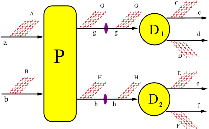
Figure 2: Kinematics of the double-resonant process.

On the other hand, looking into the example of the $\tau$-pair production and decay, the emission of soft and hard photons out of $W$’s definitely makes a lot of sense. However, in the case of the $W$-pair, the time separation of the production and decay stages is not that extremely long – this is why it is desirable to implement smooth analytical transition from the situation in which emission of photons with $E_{\gamma}<\Gamma_{W}$ is governed solely by the $J_{6f}^{\mu}$ currents to a situation in which the emission of photons with $E_{\gamma}>\Gamma_{W}$ gets a well-defined contribution from the intermediate $W$’s. The above situation is visualised in fig. 2 which describes a double-resonant process

$$\begin{split}&e^{-}(p_{a})+e^{+}(p_{b})\to W^{-}(p_{g})+W^{+}(p_{h})+n\gamma,\\ &W^{-}(p_{g})\to f_{c}(p_{c})+\bar{f}_{d}(p_{d})+n\gamma,\quad W^{+}(p_{h})\to f_{e}(p_{e})+\bar{f}_{f}(p_{f})+n\gamma,\end{split}$$ (3.3)

where we understand again that we may also contract any pair of the photon lines into a virtual photon exchange (loop). Here and in the following we use the following short-hand notation:

$$p_{ab}=p_{a}+p_{b},\quad p_{cd}=p_{c}+p_{d},\quad p_{ef}=p_{e}+p_{f}.$$ (3.4)

The key point is a very special way in which the recoil is implemented in the resonance propagators. To understand this problem better, let us consider first the case with one real photon $n=1$ in the two soft limit regimes: (i) semi-soft, $k^{0}\sim\Gamma\ll\sqrt{s}$ and (ii) true-soft, $k^{0}\ll\Gamma_{W}\ll\sqrt{s}$. The true-soft case (ii) is the case of the standard YFS, in which we have

$${\mathcal{M}^{(0)}}^{\mu_{1}}(k_{1})\simeq Const\;\frac{1}{p_{cd}^{2}-M^{2}}\;\frac{1}{p_{ef}^{2}-M^{2}}$$ (3.5)

$$\times\Bigg{\{}Q_{a}\frac{2p_{a}^{\mu}}{2p_{a}k_{1}}+Q_{b}\frac{2p_{b}^{\mu}}{2p_{b}k_{1}}-Q_{c}\frac{2p_{c}^{\mu}}{2p_{c}k_{1}}-Q_{d}\frac{2p_{d}^{\mu}}{2p_{d}k_{1}}-Q_{e}\frac{2p_{e}^{\mu}}{2p_{e}k_{1}}-Q_{f}\frac{2p_{d}^{\mu}}{2p_{f}k_{1}}\Bigg{\}}.$$

In eq. (3.5) there is no emission from any internal $W$ line and no dependence in the resonance propagators due to photon emission. In the semi-soft regime (i) we have to restore such a dependence in the resonance propagators, that is take into account the recoil. This cannot be done without introducing photon emission from the intermediate charged resonance into the total electromagnetic current (unless we drop the NFI corrections altogether, as we already discussed). In order to see this point more clearly, let us write down a naive extension of the formula of eq. (3.5) in the complete analogy with the CEEX for the neutral resonances, like the $Z$-boson:

$${\mathcal{M}^{(0)}_{1}}^{\mu}(k_{1}) \simeq\frac{1}{p_{cd}^{2}-M^{2}}\;\frac{1}{p_{ef}^{2}-M^{2}}\Bigg{\{}Q_{a}\frac{2p_{a}^{\mu}}{2p_{a}k_{1}}+Q_{b}\frac{2p_{b}^{\mu}}{2p_{b}k_{1}}\Bigg{\}}$$ (3.6)

$$+\frac{1}{(p_{cd}+k_{1})^{2}-M^{2}}\;\frac{1}{p_{ef}^{2}-M^{2}}\Bigg{\{}-Q_{c}\frac{2p_{c}^{\mu}}{2p_{c}k_{1}}-Q_{d}\frac{2p_{d}^{\mu}}{2p_{d}k_{1}}\Bigg{\}}$$

$$+\frac{1}{p_{cd}^{2}-M^{2}}\;\frac{1}{(p_{ef}+k_{1})^{2}-M^{2}}\Bigg{\{}-Q_{e}\frac{2p_{e}^{\mu}}{2p_{e}k_{1}}-Q_{f}\frac{2p_{d}^{\mu}}{2p_{f}k_{1}}\Bigg{\}}.$$

The above extension is, however, useless, because it is not gauge invariant. We have to restore emission from the internal $W$ in order to cure the gauge invariance, while maintaining recoil in the resonance propagator!

We therefore restore photon emission from the internal $W$ in the soft photon approximation (starting from Feynman diagrams) and next, factorise it into the product of the emission factors using the identity (A.2) given in Appendix A. This identity also shows why it is necessary to sum up coherently over two photon assignments, either to $W$ in the production or to $W$ in the decay.

For the single real semi-soft photon under consideration, we obtain immediately the following gauge-invariant amplitude being the sum of three parts, each of them gauge invariant by itself:

$${\mathcal{M}^{(0)}_{1}}^{\mu}(k_{1})\simeq$$ (3.7)

$$\frac{1}{p_{cd}^{2}-M^{2}}\;\frac{1}{p_{ef}^{2}-M^{2}}\Bigg{\{}Q_{a}\frac{2p_{a}^{\mu}}{2p_{a}k_{1}}+Q_{b}\frac{2p_{b}^{\mu}}{2p_{b}k_{1}}-Q_{g}\frac{2p_{g}^{\mu}}{2p_{g}k_{1}}-Q_{h}\frac{2p_{h}^{\mu}}{2p_{h}k_{1}}\Bigg{\}}$$

$$+\frac{1}{(p_{cd}+k_{1})^{2}-M^{2}}\;\frac{1}{p_{ef}^{2}-M^{2}}\Bigg{\{}Q_{g}\frac{2p_{g}^{\mu}}{2p_{g}k_{1}}-Q_{c}\frac{2p_{c}^{\mu}}{2p_{c}k_{1}}-Q_{d}\frac{2p_{d}^{\mu}}{2p_{d}k_{1}}\Bigg{\}}$$

$$+\frac{1}{p_{cd}^{2}-M^{2}}\;\frac{1}{(p_{ef}+k_{1})^{2}-M^{2}}\Bigg{\{}Q_{h}\frac{2p_{h}^{\mu}}{2p_{h}k_{1}}-Q_{e}\frac{2p_{e}^{\mu}}{2p_{e}k_{1}}-Q_{f}\frac{2p_{f}^{\mu}}{2p_{f}k_{1}}\Bigg{\}}$$

$$=\frac{1}{p_{cd}^{2}-M^{2}}\;\frac{1}{p_{ef}^{2}-M^{2}}\Bigg{\{}j^{\mu}_{P}+\frac{p_{cd}^{2}-M^{2}}{(p_{cd}+k_{1})^{2}-M^{2}}\;j^{\mu}_{D_{1}}+\frac{p_{ef}^{2}-M^{2}}{(p_{ef}+k_{1})^{2}-M^{2}}\;j^{\mu}_{D_{2}}\Bigg{\}}$$

$$=\sum_{\wp=(P,D_{1},D_{2})}^{3}\frac{1}{p_{G}^{2}-M_{W}^{2}}\frac{1}{p_{H}^{2}-M_{W}^{2}}j_{\wp}^{\mu},$$

where $p_{g}=p_{c}+p_{d}+k_{1}$ and $p_{h}=p_{e}+p_{f}+k_{1}$. In the last line we have used

$$p_{G}=p_{c}+p_{d}+K_{D_{1}},~{}~{}p_{H}=p_{e}+p_{f}+K_{D_{2}},~{}~{}K_{X}=\sum_{i\in X}k_{i}$$ (3.8)

$$j_{P}^{\mu_{i}}=\frac{2p_{a}^{\mu_{i}}}{2p_{a}k_{i}}+\frac{2p_{b}^{\mu_{i}}}{2p_{b}k_{i}}-\frac{2p_{G}^{\mu_{i}}}{2p_{G}k_{i}}-\frac{2p_{H}^{\mu_{i}}}{2p_{H}k_{i}},$$

$$j_{D_{1}}^{\mu_{i}}=\frac{2p_{G}^{\mu_{i}}}{2p_{G}k_{i}}-\frac{2p_{c}^{\mu_{i}}}{2p_{c}k_{i}}-\frac{2p_{d}^{\mu_{i}}}{2p_{d}k_{i}},~{}~{}j_{D_{2}}^{\mu_{i}}=\frac{2p_{H}^{\mu_{i}}}{2p_{H}k_{i}}-\frac{2p_{e}^{\mu_{i}}}{2p_{e}k_{i}}-\frac{2p_{f}^{\mu_{i}}}{2p_{f}k_{i}}.$$

We keep in mind that in general $p_{g,h}^{2}\neq M^{2}$. The strange looking notation in the last line with the sum over partitions assigning photon to production or decays is done for the purpose of easy generalisation to the $n$-emissions case.

The single-photon amplitude of eq. (3.7) coincides precisely (up to fermion spinors) with the $n=1$ case of the multiphoton ${\cal O}(\alpha^{0})_{exp}$ amplitude of eq. (4.10) in the next section. It features a proper dependence of the resonance propagators on the photon momentum in the entire photon energy region $k^{0}\ll\sqrt{s}$, including $k^{0}\sim\Gamma_{W}$, and interpolates smoothly with the classic YFS formula of eq. (3.5), in the limit $k^{0}\ll\Gamma_{W}$. The same will be true for the amplitude of eq. (4.10) in a more general case of $n>1$.

Let us close this section with the multiple-photon extension of the formula (3.7) with the notation of (3.8) (details of its derivation can be found in Appendix B):

$${\mathcal{M}^{(0)}_{N}}^{\mu_{1},\dots,\mu_{N}}(k_{1},\dots,k_{N})\simeq\sum_{\wp=(P,D_{1},D_{2})^{N}}^{3^{N}}\frac{1}{p_{G}^{2}-M_{W}^{2}}\frac{1}{p_{H}^{2}-M_{W}^{2}}\prod_{i=1}^{N}j_{\wp_{i}}^{\mu_{i}}.$$ (3.9)

4 CEEX scheme for charged unstable emitters

In the following we shall implicitly assume that IR-singularities are regularised with the photon mass $m_{\gamma}$. The exact IR cancellations between the real photons phase-space integrals $\int_{m_{\gamma}}d\Phi$ and the virtual form-factor $\alpha B(m_{\gamma})$ work very schematically as follows:

$$\sigma=\sum_{n=0}^{\infty}\frac{1}{n!}\int_{m_{\gamma}}d\Phi_{4+n}(k_{1}\dots k_{n})\sum_{spin}|e^{\alpha B(m_{\gamma})}\mathfrak{M}(k_{1}\dots k_{n})|^{2}.$$ (4.1)

One may, of course, introduce the traditional IR-cut $E_{\gamma}>E_{\min}$ for all real photons, see refs. [18, 25] for details. This we shall not do in the following, because it would obscure notation and is in fact unnecessary (even in the MC realisation we could stick to the $m_{\gamma}$ regulator).

In the following we shall present the formalism of CEEX for $e^{-}e^{+}\to W^{+}W^{-},\;\;W^{\pm}\to X^{\pm}$. However, this formalism is quite general and applies also to the single-$W^{\pm}$ production and decay (also in hadron–hadron collisions) and also to any other process with any unstable intermediate charged particles of arbitrary spin.

4.1 Non-resonant variant of ${\cal O}(\alpha^{1})$ CEEX for $e^{-}e^{+}\to 4f$

Let us start from defining CEEX for the $e^{-}e^{+}\to 4f$ process with the simplest possible variant of ${\cal O}(\alpha^{1})$ CEEX, in which the exponentiation procedure is not influenced by the presence of any narrow charged resonances in the Born matrix element $M^{(0)}$. This CEEX_B scheme (according to the notation introduced in Subsection 3.1) can be used for the non-resonant background in the $e^{-}e^{+}\to 4f$ process. It is a kind of warm-up example in which we introduce some notation and terminology employed in the following.

Suppressing momenta and spin indices of the fermions, the ${\cal O}(\alpha^{0})_{exp}$ and ${\cal O}(\alpha^{1})_{exp}$ $n$-photon spin amplitudes can be written in a straightforward way

$${\mathcal{M}^{(0)}_{n}}^{\mu_{1},\mu_{2},...\mu_{n}}(k_{1},k_{2},...k_{n})=\frac{1}{n!}e^{\alpha B_{6}^{\rm YFS}}\;\hat{\beta}_{0}^{(0)}\prod_{i=1}^{n}j^{\mu_{i}}(k_{i}),\qquad\hat{\beta}_{0}^{(0)}=M^{(0)},$$ (4.2)

$${\mathcal{M}^{(1)}_{n}}^{\mu_{1},\mu_{2},...\mu_{n}}(k_{1},k_{2},...k_{n})=\frac{1}{n!}e^{\alpha B_{6}^{\rm YFS}}\Bigg{\{}\hat{\beta}_{0}^{(1)}\prod_{i=1}^{n}j^{\mu_{i}}(k_{i})+\sum_{j=1}^{n}\hat{\beta}_{1}^{(1)}{}^{\mu_{j}}(k_{j})\prod_{i\neq j}j^{\mu_{i}}(k_{i})\Bigg{\}},$$

where the total electric current

$$j^{\mu}(k_{i})=ie\sum_{X=a,b,c,d,e,f}\hat{j}_{X}^{\mu}(k_{i}),\qquad\hat{j}_{X}^{\mu}(k_{i})\equiv Q_{X}\theta_{X}\frac{2p_{X}^{\mu}}{2p_{X}k_{i}},$$ (4.3)

sums contributions from all six external fermions $X=a,b,...f$, see fig. 1, and $\theta_{X}=+1$ for the incoming particle $X$ (in the initial state), $\theta_{X}=-1$ for the outgoing particle $X$ (in the final state). No emission from $W$’s is seen in $j^{\mu}$. The IF-finite $\beta$-functions are defined in the usual way

$$\hat{\beta}^{(1)}_{0}=\left[e^{-\alpha B_{6}^{\rm YFS}}M^{(0)}_{0}\right]_{{\cal O}(\alpha^{1})},$$ (4.4)

$${\hat{\beta}^{(1)}_{1}}{}^{\mu}(k)={M^{(1)}_{1}}^{\mu}(k)-j^{\mu}(k)M^{(0)}_{0}.$$

The UV-finite, IR-divergent, gauge-invariant YFS form-factor is defined in the standard way, see also Appendix C:

$$B_{6}^{\rm YFS}=\int\frac{i}{(2\pi)^{3}}\frac{d^{4}k}{k^{2}-m_{\gamma}^{2}+i\varepsilon}\;J^{\mu}(k)\circ J_{\mu}(k),$$ (4.5)

$$J^{\mu}(k)=\sum_{X=a,b,c,d,e,f}\hat{J}_{X}^{\mu}(k),\qquad\hat{J}_{X}^{\mu}(k)\equiv Q_{X}\theta_{X}\;\frac{2p_{X}^{\mu}\theta_{X}+k^{\mu}}{k^{2}+2p_{X}k\theta_{X}+i\varepsilon},$$

where $\theta_{X}$ is defined as above, and we use the following short-hand notation:

$$S(k)=J(k)\circ J(k)=\sum_{{X=a,b,c,d,e,f}\atop{Y=a,b,c,d,e,f}}J_{X}(k)\circ J_{Y}(k),$$ (4.6)

$$J_{X}(k)\circ J_{Y}(k)\equiv J_{X}(k)\cdot J_{Y}(-k),\;{\rm for}\;X\neq Y,\quad$$

$$J_{X}(k)\circ J_{X}(k)\equiv J_{X}(k)\cdot J_{X}(k).$$

As we see, $B_{6}^{\rm YFS}$ sums up the contributions from all six external fermions. IR-cancellations occur after squaring, spin-summing and integrating over the phase space, in a way which was shown using several methods in refs. [18, 25]

4.2 Resonant variant of CEEX ${\cal O}(\alpha^{1})$ for $e^{-}e^{+}\to 4f$

In the following we shall discuss the ${\cal O}(\alpha^{1})$ variant of CEEX for $e^{-}e^{+}\to 4f$ in which the recoil in resonance propagators is realised at any perturbative order and the $\Gamma_{W}/M_{W}$ suppression of the NFI contributions is a natural, built-in feature, valid in every perturbative order ${\cal O}(\alpha^{r})_{exp}$, $r=0,1,2,...$. In order to formulate such a scheme completely, one has to re-consider the isolation of IR-singular photon-emission factor to infinite order from the internal $W$ lines, going beyond the scope of the classic scheme of YFS [18]. The important element of the isolation of the apparent IR-singularities due to emission of photons from the resonant charged particles is the reorganisation of the product of the internal propagators, derived in Appendix A. The virtual exponential form-factor has also a more complicated structure and is re-derived in Appendix C. Our derivation of the CEEX amplitudes is based on rearrangement of the infinite perturbative expansion in terms of Feynman diagrams, as in refs [18, 25] and the use of the pole-expansion. Although our aim are the ${\cal O}(\alpha^{1})_{\rm CEEX}$ amplitudes, the main features of the scheme can already be defined and discussed for the simpler ${\cal O}(\alpha^{0})_{\rm CEEX}$ case, which will be discussed first. The extension of the presented technique to ${\cal O}(\alpha^{2})_{\rm CEEX}$ with the complete non-soft second-order photonic corrections and the genuine EW corrections is straightforward.

4.2.1 Introductory double-pole ${\cal O}(\alpha^{0})$ CEEX

Let us assume that for the $e^{-}e^{+}\to 4f$ process depicted in fig. 1 we have at our disposal the Born matrix element ${\cal M}^{(0)}_{0}$ which we expand into the non-pole part ${M}^{(0)}_{0}()$, the single-pole part $M^{(0)}_{0}(Q)$ and the double-pole part $M^{(0)}_{0}(Q,R)$, where $Q$ and $R$ are four-momenta in the $W$ propagators

$${{\cal M}^{(0)}_{0}}^{\mu}()={M^{(0)}_{0}}^{\mu}()+{M^{(0)}_{0}}^{\mu}(Q)+{M^{(0)}_{0}}^{\mu}(Q,R),$$ (4.7)

The same pole-expansion is done for the exact single-photon spin amplitudes

$${{\cal M}^{(1)}_{1}}^{\mu}(k)={M^{(1)}_{1}}^{\mu}(k)+{M^{(1)}_{1}}^{\mu}(Q,k)+{M^{(1)}_{1}}^{\mu}(Q,R,k),$$ (4.8)

where $k$ is the photon four-momentum and the index $\mu$ is understood to be contracted with the photon polarisation vector. The one-loop corrected complete ${\cal O}(\alpha^{1})$ spin amplitudes in the POE we denote as $M^{(1)}_{0}()$, $M^{(1)}_{0}(Q^{2})$ and $M^{(1)}_{0}(Q,R)$:

$${{\cal M}^{(1)}_{0}}^{\mu}={M^{(1)}_{0}}^{\mu}()+{M^{(1)}_{0}}^{\mu}(Q)+{M^{(1)}_{0}}^{\mu}(Q,R).$$ (4.9)

Let us focus now on the double-resonant part of the amplitudes ${M^{(0)}_{0}}^{\mu}(Q,R)$ and ${M^{(1)}_{0}}^{\mu}(Q,R)$. The single-resonant part is completely analogous (we shall list the differences) and the non-resonant case has already been discussed in the previous subsection.

The CEEX ${\cal O}(\alpha^{0})$ spin amplitudes for $n$ photons can be derived as the following gauge-invariant subset of the complete perturbative series

$${\mathcal{M}^{(0)}_{n}}^{\mu_{1},\mu_{2},...,\mu_{n}}(k_{1},k_{2},...,k_{n})=\sum_{\wp\in\{P,D_{1},D_{2}\}^{n}}\!\!\!\!\!\!e^{\alpha B_{10}(U_{\wp},V_{\wp})}\;\hat{\beta}^{(0)}_{0}\left(U_{\wp},V_{\wp}\right)\prod_{i=1}^{n}\;j_{\{\wp_{i}\}}^{\mu_{i}}(k_{i}),$$ (4.10)

$$U_{\wp}=p_{c}+p_{d}+\sum_{\wp_{i}=D_{1}}k_{i},\quad V_{\wp}=p_{e}+p_{f}+\sum_{\wp_{i}=D_{2}}k_{i}.$$

Here, the fermion four-momenta $p_{A}$ and helicities $\lambda_{A},A=a,b,c,d,e,f$ are suppressed. Photons are grouped into three sets: production, first decay and second decay, denoted as $P,D_{1},D_{2}$. The coherent sum is taken over all $3^{n}$ assignments of a photon to 3 stages of the process. Each assignment is represented by the vector $(\wp_{1},...,\wp_{n})$ whose components are taking three possible values $\wp_{j}=P,D_{1},D_{2}$. The cornerstone of this construction are three gauge invariant electric currents

$$j^{\mu}_{P}(k_{i})=ie\sum_{X=a,b,g,h}\hat{j}^{\mu}_{X}(k),\quad j^{\mu}_{D_{1}}(k_{i})=ie\sum_{X=g,c,d}\hat{j}^{\mu}_{X}(k),\quad j^{\mu}_{D_{2}}(k_{i})=ie\sum_{X=h,e,f}\hat{j}^{\mu}_{X}(k),\quad$$ (4.11)

$$p_{g}=U_{\wp},\quad p_{h}=V_{\wp},$$

defined in terms of elementary currents $\hat{j}_{X}(k)$ of eq. (4.3). They include also $\hat{j}$’s for two $W$’s, see eq. (4.3). The essential steps in derivation of the CEEX formula of eq. (4.10) are given in Appendices A, B and C.

The dependence of the amplitude in eq. (4.10) on the four-momenta was already analysed in the case of the single real photon in the previous section. The case of many real photons is completely analogous. Let us turn now our attention to a more interesting case of multiple virtual photos which contribute to the virtual form-factor $\exp(B_{10})$.

The virtual IR-singularities factorise off in eq. (4.10) into the factor $\exp(B_{10})$. Let us recall that our aim is to reproduce the $\Gamma/M$ suppression of the NFI corrections already at the ${\cal O}(\alpha^{0})_{exp}$ level. It would be incorrect to employ here the classic YFS form-factor $B_{6}^{\rm YFS}$ of eq. (4.5). This choice would render eq. (4.10) IR-finite, however, it would fail to resum the $\alpha\ln(\Gamma/M)$ contributions and miss the $\Gamma/M$ suppression of NFI corrections, at the ${\cal O}(\alpha^{0})_{exp}$ level. How to see it? One may check it by explicit analytical calculation, similar to the one performed in ref. [25], or numerically. Quite generally, the reason for the above failure is that the effective energy scale for NFI is not $\sqrt{s}$ but $\Gamma_{W}$. The NFI contributions for the real photon energies above $\Gamma_{W}$ are suppressed strongly by the resonance propagator. However, this works for the real but not for virtual photons in $B_{6}^{YFS}$, hence the energy scale for virtual photons is necessarily $\sqrt{s}$. The mismatch between the scale for real and virtual photon will cause the NFI contribution to blow up at the ${\cal O}(\alpha^{0})_{exp}$ by orders of magnitude, and even for ${\cal O}(\alpha^{1})_{exp}$ they may be far from the reality.

The remedy for the above problem is well known for the neutral resonances [48, 49, 25] and also can be deduced from the ${\cal O}(\alpha^{1})$ calculation (without exponentiation) of the NFI term for the charged resonance of $W$, see refs. [50, 39, 51]. The modified CEEX form-factor which should be used in eq. (4.10) is the following:

$$B_{10}(p_{cd},p_{ef})=\int\frac{i}{(2\pi)^{3}}\;\frac{d^{4}k}{k^{2}-\lambda^{2}+i\varepsilon}\;$$ (4.12)

$$\qquad\bigg{\{}J_{P}(k)\circ J_{P}(k)+J_{D_{1}}(k)\circ J_{D_{1}}(k)+J_{D_{2}}(k)\circ J_{D_{2}}(k)$$

$$\qquad+\frac{p_{cd}^{2}-M^{2}}{(p_{cd}-k)^{2}-M^{2}}\;2J_{P}(k)\circ J_{D_{1}}(k)+\frac{p_{ef}^{2}-M^{2}}{(p_{ef}-k)^{2}-M^{2}}\;2J_{P}(k)\circ J_{D_{2}}(k)$$

$$\qquad+\frac{p_{cd}^{2}-M^{2}}{(p_{cd}+k)^{2}-M^{2}}\;\frac{p_{ef}^{2}-M^{2}}{(p_{ef}-k)^{2}-M^{2}}\;2J_{D_{1}}(k)\circ J_{D_{2}}(k)\bigg{\}},$$

where

$$J^{\mu}_{P}(k)=\sum_{X=a,b,g,h}\hat{J}_{X}^{\mu}(k),\qquad J^{\mu}_{D_{1}}(k)=\sum_{X=g,c,d}\hat{J}_{X}^{\mu}(k),\qquad J^{\mu}_{D_{2}}(k)=\sum_{X=h,e,f}\hat{J}_{X}^{\mu}(k),$$ (4.13)

$$p_{g}=p_{cd}+K_{1},\quad p_{h}=p_{ef}+K_{2},$$

see eq. (4.6) for definition of elementary virtual current $\hat{J}_{X}$ and of its circle-products. In eq. (4.10) the four-momenta $U_{\wp},V_{\wp}$ in $B_{10}(U_{\wp},V_{\wp})$ should be identified with $p_{cd}+K_{1}$ and $p_{ef}+K_{2}$ in eq. (4.12), where $K_{1}$ and $K_{2}$ are total four momenta of all real photons in the two decay processes. Note that the above form-factor is gauge invariant and UV-finite. Moreover, each of its six components is also separately gauge invariant and UV-finite. Almost all its components are already available in the literature. We have omitted from discussion the important Coulomb effect, see ref. [39, 34] for more details.

The index $10$ in $B_{10}$ reflects the fact that we have $10$ emission currents in $B_{10}$: $6$ for fermions and $4$ for $W$’s – that is $2$ for $W$’s in the production and $2$ for $W$’s in the decays.

Heuristic derivation of the above CEEX form-factor, directly from the Feynman diagram, is done in Appendix C using similar techniques as in Subsection 3.2.2 of ref. [25]. In this derivation one may see explicitly why the first three components for the production and decays are exactly like in the standard YFS scheme, while three interferences are modified.

4.2.2 The ${\cal O}(\alpha^{1})$ CEEX for double-pole component

The construction of ${\cal O}(\alpha^{0})_{exp}$ for the $e^{+}e^{-}\to 4f$ process of the previous subsection was based, on one hand, on the gauge invariant POE of the Born spin amplitudes into the double-, single- and non-pole parts and, on the other hand, on the soft photon approximation in which real and virtual photon emission/absorption is represented as a product of the universal (spin-independent) factors, taking care of the recoil in all resonance propagators.

We intend now to extend the above scheme in such a way that the complete ${\cal O}(\alpha^{1})$ to the $e^{+}e^{-}\to 4f$ process are or can be included. The immediate question is to what extent POE into the double-, single- and non-pole parts can be kept at all at ${\cal O}(\alpha^{1})$?

Concerning POE at ${\cal O}(\alpha^{1})$, we assume that both the ${\cal O}(\alpha^{1})$ amplitudes: $M_{1}^{(1)\mu}(k)$ with the emission of an additional single photon and $M_{0}^{(1)}$ with the complete one-loop corrections can be pole-expanded into the double-, single- and non-pole parts. Obviously, this can be done in many ways. Essentially it can be done (in principle) because the two propagators for the internal $W$ line due to photon emission can always be replaced by a sum of “two poles” using the identity of eq. (A.2). Each of these terms can be made gauge invariant by taking a residue value for the entire expression multiplying the pole term, or more selectively, in its scalar part. This can be done (in principle) for both the amplitudes $M_{1}^{(1)\mu}(k)$ and $M_{0}^{(1)}$ representing the exact results of the Feynman diagrams at ${\cal O}(\alpha^{1})$. The soft-photon-approximated universal part is already included in the calculation due to the exponentiation, in the same way as at ${\cal O}(\alpha^{0})$.

The double-pole ${\cal O}(\alpha^{1})$ CEEX amplitude, including terms of ${\cal O}(\frac{\alpha}{\pi}\frac{\Gamma}{M})$ due to the NFI interferences, reads as follows:

$${\mathcal{M}^{(1)}_{n}}^{\mu_{1},\mu_{2},...,\mu_{n}}(k_{1},k_{2},...,k_{n})_{\rm DP}=\sum_{\wp\in\{P,D_{1},D_{2}\}^{n}}\!\!\!\!e^{\alpha B_{10}(U_{\wp},V_{\wp})}\hat{\beta}^{(1)}_{0}\left(U_{\wp},V_{\wp}\right)\prod_{i=1}^{n}\;j_{\{\wp_{i}\}}^{\mu_{i}}(k_{i})\;$$ (4.14)

$$\qquad+\sum_{j=1}^{n}\;\;\sum_{\wp\in\{P,D_{1},D_{2}\}^{n-1}}\!\!\!\!e^{\alpha B_{10}(U_{\wp},V_{\wp})}\hat{\beta}^{(1)\mu_{j}}_{1\{\wp_{j}\}}\left(U_{\wp},V_{\wp},k_{j}\right)\prod_{i\neq j}\;j_{\{\wp_{i}\}}^{\mu_{i}}(k_{i}),$$

where

$$\hat{\beta}^{(1)\mu}_{1}(U,V,k)=M^{(1)\mu}_{1}(U,V,k)-\sum_{\wp=P,D1,D2}j_{\wp}^{\mu}(k)M^{(0)}_{0}(U_{\wp},V_{\wp}).$$ (4.15)

The IR-finite $\hat{\beta}_{0}$-functions is here defined as follows:

$$\hat{\beta}^{(1)}_{0}(U,V)=\left[e^{-\alpha B_{10}(U,V)}M^{(1)}_{0}(U,V)\right]_{{\cal O}(\alpha^{1})}=M^{(1)}_{0}(U,V)-B_{10}(U,V)M^{(0)}_{0}(U,V),$$ (4.16)

where $B_{10}(U,V)$ is the complete variant of eq. (4.12) and the one-loop corrections in the double-pole $M^{(1)}_{0}(U,V)$ have to be complete at the ${\cal O}(\alpha^{1})$, including terms of ${\cal O}(\frac{\alpha}{\pi}\frac{\Gamma}{M})$. Special care should be taken in order to preserve gauge invariance. Infrared regulation using $m_{\gamma}$ or any other method may be employed in the intermediate steps, but the final $B_{10}(U,V)$ will be IR-finite.

Needless to say that in the above expressions, as usual in all resummation schemes, one has to provide a recipe for extrapolating the ${\cal O}(\alpha^{1})$ results, originally defined in the phase space with zero or one real photon, to the phase space enriched with many additional “spectator” photons. The uncertainty due to freedom in this extrapolation is of the ${\cal O}(\alpha^{2})$ class.

4.2.3 ${\cal O}(\alpha^{1})$ CEEX for single-pole component

The above implementation of ${\cal O}(\alpha^{1})$ CEEX for the DP component of the QED ${\cal O}(\alpha^{1})$ corrections are complete including ${\cal O}(\frac{\alpha}{\pi}\frac{\Gamma}{M})$ corrections due the NFI interferences. However, the ${\cal O}(\frac{\alpha}{\pi}\frac{\Gamma}{M})$ corrections arise also from the entire QED ${\cal O}(\alpha^{1})$ correction to a single-pole component (which by itself is of ${\cal O}(\frac{\Gamma}{M})$). It is therefore necessary to define ${\cal O}(\alpha^{1})$ CEEX for the SP part. In addition, CEEX for the SP process is also of the vital importance for the $q\bar{q}\to W\to f\bar{f}$ process at hadron colliders, such as the LHC.

On the other hand, the non-pole (background) part, which is of ${\cal O}((\frac{\Gamma}{M})^{2})$), may included without QED corrections or any kind of implementation of QED corrections, for instance using the simple baseline ${\cal O}(\alpha^{0})$ CEEX version of Subsection 4.2.1.

The CEEX ${\cal O}(\alpha^{1})_{exp}$ single-pole and double-pole spin amplitudes will be combined additively as follows:

$${\mathcal{M}^{(1),\mu_{1},\dots,\mu_{n}}_{n}}(k_{1},k_{2},...,k_{n})_{\rm DSP}={\mathcal{M}^{(1),\mu_{1},\dots,\mu_{n}}_{n}}(k_{1},k_{2},...,k_{n})_{\rm SP}+{\mathcal{M}^{(1),\mu_{1},\dots,\mu_{n}}_{n}}(k_{1},k_{2},...,k_{n})_{\rm DP}.$$ (4.17)

The single-pole ${\mathcal{M}^{(1)}_{n}(\ldots)_{\rm SP}}$ amplitude is constructed analogously as in eq. (4.10). The differences are that: (i) the current $j^{\mu}_{P}$ in the production process $e^{+}e^{-}\to f_{c}+\bar{f}_{d}+W^{+}$ has five components instead of four, (ii) the function $B_{8}$ replaces $B_{10}$, the $B_{8}$ has less components, in particular one interference term instead of three, (ii) the sum over photon assignment is reduced to the sum over the set $\{\wp\}=(P,D_{1})^{n}$ corresponding to $2^{n}$ assignments:

$${\mathcal{M}^{(1)}_{n}}^{\mu_{1},\mu_{2},...,\mu_{n}}(k_{1},k_{2},...,k_{n})_{SP}=\sum_{\wp\in\{P,D_{1}\}^{n}}\!\!\!\!e^{\alpha B_{8}(U_{\wp})}\hat{\beta}^{(1)}_{0}\left(U_{\wp}\right)\prod_{i=1}^{n}\;j_{\{\wp_{i}\}}^{\mu_{i}}(k_{i})\;$$ (4.18)

$$\qquad\qquad\qquad+\sum_{j=1}^{n}\;\sum_{\wp\in\{P,D_{1}\}^{n-1}}\!\!\!\!e^{\alpha B_{8}(U_{\wp})}\hat{\beta}^{(1)\mu_{j}}_{1\{\wp_{j}\}}\left(U_{\wp},k_{j}\right)\prod_{i\neq j}\;j_{\{\wp_{i}\}}^{\mu_{i}}(k_{i}),$$

where

$$\hat{\beta}^{(1)\mu}_{1}(U,k)=M^{(1)\mu}_{1}(U,k)-\sum_{\wp=P,D1}j_{\wp}^{\mu}(k)M^{(0)}_{0}(U_{\wp}).$$ (4.19)

The IR-finite $\hat{\beta}_{0}$-functions is defined here as follows:

$$\hat{\beta}^{(1)}_{0}(U)=\left[e^{-\alpha B_{8}(U)}M^{(1)}_{0}(U)\right]_{{\cal O}(\alpha^{1})}=M^{(1)}_{0}(U)-B_{8}(U)M^{(0)}_{0}(U),$$ (4.20)

where $M^{(1)}_{0}(U)$ is the single-pole part in the Born amplitude of the $e^{+}e^{-}\to 4f$ process and the one-loop corrected single-pole $M^{(1)}_{0}(U)$ amplitude is complete at ${\cal O}(\alpha^{1})$. The $B_{8}(U)$ function is the following variant of that in eq. (4.12):

$$B_{8}(p_{cd})=ie\int\frac{i}{(2\pi)^{3}}\;\frac{d^{4}k}{k^{2}-\lambda^{2}+i\varepsilon}\;$$ (4.21)

$$\qquad\bigg{\{}J_{P}(k)\circ J_{P}(k)+J_{D_{1}}(k)\circ J_{D_{1}}(k)+\frac{p_{cd}^{2}-M^{2}}{(p_{cd}+k)^{2}-M^{2}}\;2J_{P}(k)\circ J_{D_{1}}(k)\bigg{\}}.$$

The above ${\cal O}(\alpha^{1})$ CEEX for the single-pole part of the $e^{+}e^{-}\to 4f$ process implemented in $\mathcal{M}^{(1)}_{n}(\ldots)_{\rm SP}$ provides, together with the double-pole CEEX amplitude $\mathcal{M}^{(1)}_{n}(\ldots)_{\rm DP}$ of the previous section, the complete QED corrections at the order of ${\cal O}(\alpha^{1})$, ${\cal O}(\frac{\Gamma}{M})$ and ${\cal O}(\frac{\alpha}{\pi}\frac{\Gamma}{M})$ for the $e^{+}e^{-}\to 4f$ process. Let us keep in mind that the definition of the ${\cal O}(\frac{\alpha}{\pi}\frac{\Gamma}{M})$ terms in $\mathcal{M}^{(1)}_{n}(\ldots)_{\rm SP}$ and $\mathcal{M}^{(1)}_{n}(\ldots)_{\rm DP}$ depends on the exact definition of the SP and DP components in POE. Only the sum of them is uniquely defined – more precisely up to the terms of ${\cal O}(\frac{\alpha}{\pi}(\frac{\Gamma}{M})^{2})$.

In the above formalism, the fermions labeled $e$ and $f$ do not form the resonance. In the case of the single-$W$ production in the quark–antiquark annihilation in hadron–hadron collision, the same formalism applies but the particles $e$ and $f$ are just absent.

4.2.4 Approximate version of ${\cal O}(\alpha^{1})$ CEEX

Let us also consider one simpler case of the CEEX matrix element, with the incomplete ${\cal O}(\frac{\alpha}{\pi}\frac{\Gamma}{M})$ corrections. It may be of some practical significance for applications with limited precision and will be described for the DP part only.

In this alternative scheme, the ${\cal O}(\alpha^{0})$ part is kept the same as in the full version of the CEEX scheme for the DP part of Subsection 4.2.2. The main difference is in the simplification of the non-soft ${\cal O}(\alpha^{1})$ remnants, in which the non-factorisable QED interferences between the production and the decays are downgraded to the soft-photon approximation.

In such an approximation, the ${\cal O}(\alpha^{1})$ non-soft corrections are calculated separately for the production and two decay processes, and they contribute separately and additively to both real $\hat{\beta}^{(1)\mu_{1}}$ and virtual $\hat{\beta}^{(1)\mu}_{0}$:

$$\hat{\beta}^{(1)\mu}_{1}(U,V,k)=\sum_{X=P,D_{1},D_{2}}\hat{\beta}^{(1)\mu}_{1,X}(U,V,k),\quad\hat{\beta}^{(1)}_{0}(U,V)=\sum_{X=P,D_{1},D_{2}}\hat{\beta}^{(1)}_{0,X}(U,V),$$ (4.22)

where $U=p_{cd}$, $V=p_{ef}$. For instance, the non-soft contributions from penta-box diagrams in the NFI class are neglected completely in the $\hat{\beta}^{(1)}_{0}(U,V)$, because their soft part (including resonance effects) is already included in the $B_{10}(U,V)$ function. The single real photon emission spin amplitudes factorise into the production and decay parts

$$\mathcal{M}_{1}^{(1)\mu}(k)=\mathcal{M}_{1,P}^{(1)\mu}(k)\;\mathcal{M}_{0,D_{1}}^{(0)}\;\mathcal{M}_{0,D_{2}}^{(0)}+\mathcal{M}_{1,P}^{(0)}\;\mathcal{M}_{1,D_{1}}^{(1)\mu}(k)\;\mathcal{M}_{0,D_{2}}^{(0)}+\mathcal{M}_{1,P}^{(0)}\;\mathcal{M}_{0,D_{1}}^{(0)}\;\mathcal{M}_{1,D_{2}}^{(1)\mu}(k)\;$$ (4.23)

$$=\mathcal{M}_{0,P}^{(0)}\big{[}j_{P}^{\mu}(k)\mathcal{M}_{0,D_{1}}^{(0)}\mathcal{M}_{0,D_{2}}^{(0)}+\mathcal{M}_{0,D_{1}}^{(0)}(k)j_{D_{1}}^{\mu}(k)\mathcal{M}_{0,D_{2}}^{(0)}+\mathcal{M}_{0,D_{1}}^{(0)}\mathcal{M}_{0,D_{2}}^{(0)}(k)j_{D_{2}}^{\mu}(k))\big{]}$$

$$~{}~{}~{}+\tilde{\beta}^{(1)\mu}_{P}(k)\mathcal{M}_{0,D_{1}}^{(0)}\mathcal{M}_{0,D_{2}}^{(0)}+\mathcal{M}_{1,P}^{(0)}\;\tilde{\beta}^{(1)\mu}_{D_{1}}(k)\mathcal{M}_{0,D_{2}}^{(0)}+\mathcal{M}_{1,P}^{(0)}\;\mathcal{M}_{0,D_{1}}^{(0)}\tilde{\beta}^{(1)\mu}_{D_{2}}(k)$$

$$=\hat{\beta}^{(0)}_{0}\left(U,V\right)j_{P}^{\mu}(k)+\hat{\beta}^{(0)}_{0}\left(U+k,V\right)j_{D_{1}}^{\mu}(k)+\hat{\beta}^{(0)}_{0}\left(U,V+k\right)j_{D_{2}}^{\mu}(k)$$

$$~{}~{}~{}+\hat{\beta}^{(1)\mu}_{1P}(k)+\hat{\beta}^{(1)\mu}_{1D_{1}}(k)+\hat{\beta}^{(1)\mu}_{1D_{2}}(k),$$

where $\tilde{\beta}^{(1)\mu}_{X}(k),\;\;X=P,D_{1},D_{2}$ are the CEEX elements for the production and the decays separately, and we have adopted a convention that the $W$ propagator is included in the lowest order decay amplitude $\mathcal{M}_{0,D_{i}}^{(0)}$. An additional argument $(k)$ in $\mathcal{M}_{0,D_{i}}^{(0)}(k)$ marks that this $W$ propagator includes the momentum $k$ of the photon emitted in the decay.

The resulting variant of the ${\cal O}(\alpha^{1})$ CEEX amplitude reads as follows:

$${\mathcal{M}^{(1)}_{n}}^{\mu_{1},\mu_{2},...,\mu_{n}}(k_{1},k_{2},...,k_{n})$$ (4.24)

$$=\!\!\!\sum_{\wp\in\{P,D_{1},D_{2}\}^{n}}\!\!\!\!\!e^{\alpha B_{10}(U_{\wp},V_{\wp})}\Bigg{\{}\hat{\beta}^{(1)}_{0}\left(U_{\wp},V_{\wp}\right)\prod_{i=1}^{n}\;j_{\{\wp_{i}\}}^{\mu_{i}}(k_{i})\;+\sum_{j=1}^{n}\hat{\beta}^{(1)\mu_{j}}_{1\{\wp_{j}\}}\left(U_{\wp},V_{\wp},k_{j}\right)\prod_{i\neq j}\;j_{\{\wp_{i}\}}^{\mu_{i}}(k_{i})\;\Bigg{\}}.$$

The important difference with respect to the previous case is that due to the splitting of $\hat{\beta}^{(1)}$ into the production and decay parts, the photon $k_{j}$ entering $\hat{\beta}^{(1)}$ is included into the sum over the photon assignments.

4.2.5 Higher order upgrades and inclusion of genuine electroweak corrections

The upgrade of the CEEX amplitudes from ${\cal O}(\alpha^{1})$ to ${\cal O}(\alpha^{2})$ is straightforward, following the same path as in the analogous case of the QED ${\cal O}(\alpha^{2})$ CEEX scheme implemented in the KKMC project[24, 25]. The CEEX scheme offers great flexibility, allowing to truncate a perturbative series at a different order for ISR, FSR, IFI and IFF. This may be exploited in a convenient staging of construction of the respective numerical Monte Carlo program. In particular, for the ISR corrections it would be good to include the LO ${\cal O}(\alpha^{3})$ corrections. From the experience of the KKMC project we know that calculations of the CEEX ${\cal O}(\alpha^{2})$ matrix element may be slow, due to the need of summations over the assignments of photons among production and decays. However, most of numerical contributions from these photon assignments are numerically negligible and one may invent methods of the effective forecasting which assignments can be omitted from the evaluation. This would speed up significantly numerical MC calculations.

In the present work we concentrate on the QED part of the SM calculations for the $e^{+}e^{-}\to W^{+}W^{-}$ process. Is it possible to factorise and treat separately the QED part from the rest of the SM corrections, the genuine EW corrections? The answer is positive because the soft-photon factorisation for both the real and virtual photons is well established in the framework of perturbative calculations [18]. The remaining genuine EW ${\cal O}(\alpha^{r})$ $r=1,2$ corrections are located in the IR-finite remnants $\hat{\beta}^{(r)\mu}_{0}$, $\hat{\beta}^{(r)\mu}_{1}(k),\hat{\beta}^{(r)\mu_{1}\mu_{2}}_{2}(k_{1},k_{2})$. It is only important to remember that the CEEX scheme works at the amplitude level and in the calculation of the loop corrections leading to $\hat{\beta}^{(r)\mu}_{0}$ or $\hat{\beta}^{(r)\mu}_{1}(k)$, all the IR divergences are removed by means of subtracting the $B_{10}$ function – adding the real emissions à la Bloch–Norsieck in order to obtain finite results is a methodological mistake! Because of that it is much easier to manage the genuine EW corrections in the CEEX scheme of any perturbative order than in any other scheme, especially beyond ${\cal O}(\alpha^{1})$.

In the KandY (YFSWW3) calculations of the LEP era, the ${\cal O}(\alpha^{1})$ genuine EW corrections were included in $\hat{\beta}^{(1)\mu}_{0}$ for the DP production part of the process (similarly as in RACOONWW). In order to match a very high precision of the FCC-ee experiments, it will be necessary to introduce the ${\cal O}(\alpha^{2})$ corrections in $\hat{\beta}^{(2)\mu}_{0}$ and $\hat{\beta}^{(1)\mu}_{1}(k)$ of the DP component. They are not available yet. In addition, it will be needed to introduce the ${\cal O}(\alpha^{1})$ EW corrections in $\hat{\beta}^{(1)\mu}_{0}$ of the SP component. This subgroup of corrections can, in principle, be extracted from the existing EW ${\cal O}(\alpha^{1})$ calculations for the entire $e^{+}e^{-}\to 4f$ process of ref.[31, 32].

5 Relations between CEEX and EEX schemes

Tracing exact relations between various CEEX and EEX schemes is quite important for at least two reasons. The EEX implementation of the exclusive exponentiation in YFSWW3 is the only existing one for the $e^{+}e^{-}\to 4f$ process, so it is desirable to show that it can be embedded in the CEEX scheme as a kind of a well-defined approximation. It will also help to better understand the physics of photon emission from unstable charged intermediate particles and the inherent limitations of the EEX exponentiation scheme in YFSWW3, in particular clarifying the question: what is exactly the mechanism of neglecting the NFI interferences in EEX of YFSWW3?

Another important reason is that it would be desirable to implement the CEEX matrix element using a MC correction weight on top of the same baseline MC distributions, which is implemented in the MC event generator for the EEX matrix element. This strategy was successfully exploited in the KKMC program and also in the KandY hybrid Monte Carlo. For these reasons it is interesting to establish the relation between the CEEX and EEX distributions all over the entire multiphoton phase space.

5.1 From CEEX_R to EEX_R algebraically

As we have already indicated in the introduction, the EEX differential distributions for the process $e^{-}e^{+}\to W^{-}W^{+},\;W^{\pm}\to f\bar{f}$, can be obtained as a limiting case of the CEEX scheme for the process $e^{-}e^{+}\to 4f$, defined in this paper. Let us do it in the following. This is analogous to the derivation of EEX of KORALZ out of the CEEX amplitudes given in Section 4 of ref. [25]. The transition to EEX of YFSWW3 requires a few additional steps described in the next subsection.

As a starting point we take an approximate variant of CEEX of eq. (4.24), which is obtained from the exact one of eq. (4.14) by means of neglecting some non-IR interference NFI terms:

$$\sigma=\frac{1}{flux}\;\sum_{n=0}^{\infty}\frac{1}{n!}\int dLips_{4+n}(p_{a}+p_{b};p_{c},p_{d},p_{e},p_{f},k_{1}...k_{n})$$ (5.1)

$$\times\!\!\!\sum_{\wp\in\{P,D_{1},D_{2}\}^{n}}\!\!\!\!\!e^{\alpha B_{10}(U_{\wp},V_{\wp})}\Bigg{\{}\hat{\beta}^{(1)}_{0}\left(U_{\wp},V_{\wp}\right)\prod_{i=1}^{n}\;j_{\{\wp_{i}\}}^{\mu_{i}}(k_{i})\;+\sum_{j=1}^{n}\hat{\beta}^{(1)\mu_{j}}_{1\{\wp_{j}\}}\left(U_{\wp},V_{\wp},k_{j}\right)\prod_{i\neq j}\;j_{\{\wp_{i}\}}^{\mu_{i}}(k_{i})\;\Bigg{\}}$$

$$\times\!\!\!\sum_{\wp^{\prime}\in\{P,D_{1},D_{2}\}^{n}}\!\!\!\!\!e^{\alpha B_{10}^{*}(U_{\wp^{\prime}},V_{\wp^{\prime}})}\Bigg{\{}\hat{\beta}^{(1)}_{0}\left(U_{\wp^{\prime}},V_{\wp^{\prime}}\right)\prod_{i=1}^{n}\;j_{\{\wp^{\prime}_{i}\}}^{\mu_{i}}(k_{i})\;+\sum_{j=1}^{n}\hat{\beta}^{(1)\mu_{j}}_{1\{\wp^{\prime}_{j}\}}\left(U_{\wp^{\prime}},V_{\wp^{\prime}},k_{j}\right)\prod_{i\neq j}\;j_{\{\wp^{\prime}_{i}\}}^{\mu_{i}}(k_{i})\;\Bigg{\}}^{*},$$

where $U_{\wp}=p_{cd}+\sum_{\wp_{i}=D_{1}}k_{i}$ and $V_{\wp}=p_{ef}+\sum_{\wp_{i}=D_{2}}k_{i}$.

The consistent method of omitting all of the remaining QED NFI interferences between the production and two decays requires omitting from the double sum over photon assignments all non-diagonal terms, $\wp\neq\wp^{\prime}$, and the interference terms in $B_{10}$. After doing that the above omission the sum over photons can be reorganised into a product of three separate sums, one for the production and two for the decays. In this way we get the following EEX expression:

$$\sigma=\frac{1}{flux}\;\sum_{n=0}^{\infty}\;\frac{1}{n!}\;\int dLips_{4+n}(p_{a}+p_{b};p_{c},p_{d},p_{e},p_{f},k_{1}...k_{n})$$ (5.2)

$$\times\!\!\sum_{\wp\in\{P,D_{1},D_{2}\}^{n}}e^{2\alpha\Re B_{PDD}(U_{\wp},V_{\wp})}\prod_{i=1}^{n}\;|j_{\{\wp_{i}\}}^{\mu_{i}}(k_{i})|^{2}\;\Bigg{\{}|\hat{\beta}^{(1)}_{0}\left(U_{\wp},V_{\wp}\right)|^{2}$$

$$+\sum_{j=1}^{n}\left(2\Re\big{(}\hat{\beta}^{(1)}_{1\{\wp_{j}\}}(U_{\wp},V_{\wp},k_{j})\cdot j_{\{\wp_{j}\}}(k_{j})^{*}\big{)}+|\hat{\beta}^{(1)}_{1\{\wp_{j}\}}(U_{\wp},V_{\wp},k_{j})|^{2}\right)|j_{\{\wp_{j}\}}(k_{j})|^{-2}\;\Bigg{\}}.$$

In the above expression the YFS form-factor $e^{2\alpha\Re B_{10}}$ factorises into the product of independent form-factors for the production and two decay processes:

$$e^{2\alpha\Re B_{PDD}}=e^{2\alpha\Re B_{P}}e^{2\alpha\Re B_{D_{1}}}e^{2\alpha\Re B_{D_{2}}}.$$ (5.3)

Eq. (5.2) can be rewritten in a more traditional EEX notation as follows:

$$\sigma=\frac{1}{flux}\;\sum_{n=0}^{\infty}\;\frac{1}{n!}\;\int dLips_{4+n}(p_{a}+p_{b};p_{c},p_{d},p_{e},p_{f},k_{1}...k_{n})\!\!\sum_{\wp\in\{P,D_{1},D_{2}\}^{n}}$$ (5.4)

$$e^{2\alpha\Re B_{PDD}(U_{\wp},V_{\wp})}\prod_{i=1}^{n}\;\tilde{S}_{\{\wp_{i}\}}(k_{i})\;\Bigg{\{}\bar{\beta}^{(1)}_{0}\left(U_{\wp},V_{\wp}\right)+\sum_{j=1}^{n}\bar{\beta}^{(1)}_{1\{\wp_{j}\}}(U_{\wp},V_{\wp},k_{j})\big{[}\tilde{S}_{\{\wp_{j}\}}(k_{j})\big{]}^{-1}\;\Bigg{\}},$$

where

$$\tilde{S}_{X}(k)=|j_{X}^{\mu}(k)|^{2},\;X=P,D_{1},D_{2}.$$ (5.5)

Note that in the above expression for each photon assignment we perfectly know the four momentum in each $W$ propagator – simply because each photon is associated with the production or one of the two decays.

In fact eq. (5.2) looks like three separate EEX exponentiation schemes for the three subprocesses. They talk to each other only through total energy conservation and spin correlations. This can be seen manifestly even more clearly when, for the purpose of the MC implementation, eq. (5.4) is transformed into the following form in which the $\tilde{S}$-factors for the production and the decays are factorised. For $n$ photons in the overall sum over $3^{n}$ assignments of the photons $\{P,D_{1},D_{2}\}^{n}$ there are groups (partitions) of $\frac{n!}{n_{0}!n_{1}!n_{2}!}$ choices, with $n_{0}$ photons in the production, $n_{1}$ photons in the first decay and $n_{2}$ photons in the second decay, $n_{0}+n_{1}+n_{2}=n$. The assignments in each partition are related by the permutation of the photons within the partition. We may replace in eq. (5.4) the whole such a partition just by one permutation member, getting the following expression:

$$\sigma=\sum_{n_{0}=0}^{\infty}\sum_{n_{1}=0}^{\infty}\sum_{n_{2}=0}^{\infty}\int dLips_{4+n_{0}+n_{1}+n_{2}}(p_{a}+p_{b};p_{c},p_{d},p_{e},p_{f},k_{1}...k_{n_{2}})$$ (5.6)

$$\times\frac{1}{n_{0}!}\prod_{i_{1}=0}^{n_{0}}\;\tilde{S}_{P}(k_{i_{0}})\;\frac{1}{n_{1}!}\prod_{i_{1}=1}^{n_{1}}\;\tilde{S}_{D_{1}}(k_{i_{1}})\;\frac{1}{n_{2}!}\prod_{i_{2}=1}^{n_{2}}\;\tilde{S}_{D_{2}}(k_{i_{2}})\;$$

$$\times e^{2\alpha\Re B_{PDD}(U_{1},V_{2})}\Bigg{\{}\bar{\beta}^{(1)}_{0}\left(U_{1},V_{2}\right)+\sum_{j=1}^{n_{0}}\bar{\beta}^{(1)}_{1\{P\}}(U_{1},V_{2},k_{j})\;\tilde{S}_{P}(k_{j})^{-1}\;$$

$$+\sum_{j=1}^{n_{1}}\bar{\beta}^{(1)}_{1\{D_{1}\}}(U_{1},V_{2},k_{j})\;\tilde{S}_{D_{1}}(k_{j})^{-1}+\sum_{j=1}^{n_{2}}\bar{\beta}^{(1)}_{1\{D_{2}\}}(U_{1},V_{2},k_{j})\;\tilde{S}_{D_{2}}(k_{j})^{-1}\Bigg{\}},$$

where $U_{1}=p_{cd}+\sum_{i_{1}=0}^{n_{1}}k_{i_{1}}$ and $V_{2}=p_{ef}+\sum_{i_{2}=0}^{n_{2}}k_{i_{2}}$. One can always come back to the configuration of eq. (5.4) by means of symmetrisation over photons. In MC computations, the sum over photons is “randomised” in a natural way and only one partition member is generated at a time, (using effectively eq. (5.6)) so the fact that the basic distribution for EEX_R is that of eq. (5.4) can be easily overlooked, see also discussion in [24].

From the above algebra we see in a detail how EEX_R can be embedded in a natural way in the full CEEX_R, defined in the previous section.

5.2 Last step towards EEX_R of YFSWW3

The EEX of eq. (5.6) is not exactly that of EEX of YFSWW3 and KandY, as described in refs. [12, 9]. Let us discuss the remaining differences. The most important difference is that QED matrix element for the $W$-boson decay in YFSWW3 is implemented using the PHOTOS program whose has matrix element is not in the EEX scheme, although very close to it. At the precision of the LEP experiments this was the acceptable and economic solution. There would be no problems with replacing PHOTOS with the true EEX implementation for the $W$ decays because such an implementation is already available in the WINHAC program developed for the single-$W$ production at hadron colliders [30].

The implementation of the EEX matrix elements for the production process in YFSWW3 is described in fine detail in ref. [12]. It is based on the YFS3 event generator [27] for the $e^{+}e^{-}\to 2f$ process in which the final-state massive fermions are replaced with $W$’s. The YFS3 program does not include the QED initial-final state interferences (IFI) between initial $e^{\pm}$ and final particles. Such interferences (present in EEX of eq. (5.6) were also added in YFSWW3 using the reweighting technique of the BHWIDE program [47].

5.3 From EEX_R to CEEX_R in MC implementation

The upgrade from EEX of eq. (5.6) to CEEX in the MC implementation is feasible and well defined. In the Monte Carlo program implementing EEX, one usually generates MC events according to some baseline distribution and the final correcting weight introduces fine details of the EEX matrix element. The CEEX matrix elements can be implemented by reweighting events generated according to the same baseline distributions as in the EEX case, just by replacing the EEX final MC correcting weight with that of CEEX, without any changes in the baseline MC. This kind of flexible and economic solution was already applied in the KKMC program [24]. Similarly as in KKMC, the MC weight correcting from EEX to CEEX will be not bound from the above. There are several solutions for this purely technical problem.

5.4 Photon distributions around $E_{\gamma}\sim\Gamma$

Let us finally comments on two apparent deficiencies of the EEX_R scheme:

• lack of transmutation of photon distributions around $E_{\gamma}\sim\Gamma$,

• excess of photon-multiplicity for very soft photons, $E_{\gamma}\leq\Gamma$.

The phenomenon of “transmutation of photon distributions” occurs when photon energy changes from the “semisoft region” $\Gamma<E_{\gamma}\ll E_{beam}$ down to “true soft region” $E_{\gamma}<\Gamma$. In the true-soft region photon distributions do not reflect the existence of the the single charged object, the resonance – they reflect, instead, momenta and charges of all its decay products. For these long range photons, the resonance itself just lives too shortly to be “felt”. On the other hand, the semi-soft photons with shorter wavelength can see the resonance as a distinct object – its presence is imprinted in the distributions of photon energy and angles. In fact, it is the interference between the production-current $j^{\mu}_{P}$ and the decay-current $j^{\mu}_{D1,D2}$ which enforces the transition in the photon distributions. This effect can be also seen explicitly in the instrumental identity of eq. (A.2), or in the explicit one-photon emission amplitude of eq. (3.7). The absence of this interference in EEX, where all the NFI interferences are neglected, causes that in EEX (of YFSWW3) the above beautiful transmutation phenomenon cannot be present.

The lack of the above interferences causes also certain unphysical effect for very soft photons. As we know, in the real world (and in CEEX) there is no IR singularity (neither real nor virtual) for the photon emission from the internal $W$ line, see eq. (3.7), while in EEX there is such (real and virtual), as seen explicitly in eq. (5.6). How to explain this paradox? Is this something dangerous? The artificial IR divergence in EEX is not dangerous as long as we are at the ${\cal O}(\frac{\alpha}{\pi}\frac{\Gamma}{M})$ precision level for the distributions which are inclusive enough, such that we do not examine multiplicities and angular spectra of the photons with $E_{\gamma}<\Gamma$. Extra unphysical photons in this energy range do not contribute to integrated cross section, because their contribution is countered immediately by the virtual form-factor. They will however affect multiplicity of such very soft photons.

The good agreement of the soft photon spectra between YFSWW3 and RACOONWW confirms that the effect is not sizeable. The numerical estimates of ref. [50] also suggest that this effect is small, negligible for LEP2. On the other hand, in the future high-statistics experiments it is worth to examine the above effects for the photons with $E_{\gamma}\sim\Gamma_{W}$. It was proposed in ref. [50] that it may even provide an independent relatively precise measurement of $\Gamma_{W}$.

Summarising, the presence of the extra unphysical soft photons with $E_{\gamma}<\Gamma$ in EEX (and its version implemented in YFSWW3) due to setting to zero all QED interference effects between the production and decay processes is not harmful at the precision level of ${\cal O}(\frac{\alpha}{\pi}\frac{\Gamma}{M})$. For the higher-precision requirements, like that in FCC-ee, one should go back to CEEX_R, from which EEX_R is derived, and get back for $E_{\gamma}\sim\Gamma$ fully exclusive realistic photon distributions.

6 Summary and outlook

In the present paper we have proposed a solution to the long-standing problem of the systematic treatment of the soft and hard photon emission from the unstable charged particles and the interferences between production and decay parts of the process, at any perturbative order. This is of practical importance for high-precision measurements of $W^{+}W^{-}$-pair production at electron–positron colliders, such as FCC-ee/ILC/CLIC, and for single-$W$ production at hadron colliders, such as LHC/FCC-hh, as well as in many other processes with production and decay of charged unstable particles of any spin. So far there is no practical implementation of the full-scale calculation in the proposed scheme. However, it has been outlined how to accomplish it in the framework of some existing Monte Carlo (MC) event generators.

Our study has been focused on the process $e^{+}e^{-}\to W^{+}W^{-}\to 4f$ which is to be used e.g. for the high-precision $W$-boson mass and width measurements in the planned electron–positron colliders, particularly FCC-ee. We have argued that the most economical (and perhaps the only feasible) way to achieve the required accuracy of theoretical prediction for this process it to apply the so-called pole expansion (POE) to the general process of $e^{+}e^{-}\to 4f$, and then to calculate the electroweak (EW) radiative corrections separately for each term of such an expansion to an appropriate order in the coupling constant $\alpha$. More specifically, for the leading term in POE, i.e. the so-called double-pole contribution which comprises two resonant $W$-bosons, one would need to include the fixed-order EW corrections up to ${\cal O}(\alpha^{2})$ for the on-shell-like $W$-pair production and $W$ decay processes, while for the non-leading terms, i.e. the single-pole and non-pole contributions, the EW corrections at ${\cal O}(\alpha^{1})$ would be sufficient. The calculations of the ${\cal O}(\alpha^{1})$ EW corrections are already available for the whole $e^{+}e^{-}\to 4f$ process, while the ${\cal O}(\alpha^{2})$ ones for the double-resonant contribution do not exist yet, however they are feasible, in our opinion, by the time of the planned FCC-ee physics run.

In addition to the above fixed-order radiative corrections, in order to reach the requisite theoretical precision for the above process, one needs to include higher-order QED corrections corresponding to multiphoton emission from the initial- and final-state leptons as well as from the intermediate $W$-bosons. We have argued that the best framework in which all this can be accomplished is the so-called coherent exclusive exponentiation (CEEX) scheme. Its main advantage over the traditional YFS exclusive exponentiation (EEX) method is that it operates directly at the level of spin amplitudes. Because of that, all multiphoton effects related to radiation from the resonant $W$-bosons and to non-factorisable interferences can be accounted for in a straightforward way. So far, the CEEX methodology was applied to $e^{+}e^{-}\to 2f$ in the KKMC event generator and proved to be crucial in providing precision theoretical predictions for this process necessary for the LEP experiments.

We have provided the respective general cross-section formulae for the double-pole, single-pole and non-pole contributions to the charged-current $e^{+}e^{-}\to 4f$ process which can be a basis for an appropriate MC implementation. An important ingredient in that is resummation of real-photon emissions including radiation from the intermediate $W$-bosons and derivation of the corresponding virtual-photon form-factor, done explicitly in Appendices A, B and C. Our approach exploited the similarity between the virtual- and real-emission QED form-factors guaranteed by the infra-red cancellations.

We have also discussed the relation of the above CEEX realisation to the existing EEX implementation in terms of the hybrid MC program called KandY, being the combination of two MC event generators: KORALW and YFSWW3. In this implementation, the ${\cal O}(\alpha^{3})$ YFS exponentiation for initial-state radiation in the process $e^{+}e^{-}\to 4f$ was combined with the fixed-order ${\cal O}(\alpha^{1})$ EW corrections in the $W$-pair production and multiphoton radiation in the $W$-decays generated by the PHOTOS program, while all the non-factorisable interferences were neglected. Such a solution proved to be good enough for the LEP2 accuracy, but for the expected precision of the FCC-ee experiments it will not suffice. However, it can constitute a good starting point and a MC platform for development and implementation of the CEEX scheme described in this paper. In parallel, one can also develop an EEX approximation of the full-scale CEEX solution which will be important for its numerical cross-checks. For this, the implementation of EEX for the $W$-boson decays in the WINHAC program can be used to replace the corresponding PHOTOS radiation in KandY.

Appendix A Factoring photon-emission from $W$

The following considerations are valid for a charged unstable particle of any spin, eg. $W^{\pm}$, $\tau^{\pm}$ or $t$-quark. Let us start with a simple identity for two propagators related to single photon emission from an internal charged particle line

$$\frac{1}{(Q_{0}^{2}-M^{2})(Q_{1}^{2}-M^{2})}=\frac{1}{(Q_{0}^{2}-Q_{1}^{2})(Q_{1}^{2}-M^{2})}-\frac{1}{(Q_{0}^{2}-Q_{1}^{2})(Q_{0}^{2}-M^{2})}$$ (A.1)

where $M^{2}=M_{W}^{2}+iM_{W}\Gamma_{W}$.

The kinematics is depicted in fig 3.

Figure 3: Single emission from the internal W line.

Noticing that $Q_{0}^{2}-Q_{1}^{2}=2k_{1}Q_{0}-k_{1}^{2}=2k_{1}Q_{1}+k_{1}^{2}$, we may rewrite the above as follows:

$$\frac{1}{(Q_{0}^{2}-M^{2})(Q_{1}^{2}-M^{2})}=\frac{1}{(2k_{1}Q_{1}+k_{1}^{2})(Q_{1}^{2}-M^{2})}+\frac{1}{(-2k_{1}Q_{0}+k_{1}^{2})(Q_{0}^{2}-M^{2})}.$$ (A.2)

The reader will recognise the first term as representing a photon (eikonal) emission factor in the production part of the process times a resonance propagator (with the reduced four momentum $Q_{1}=Q_{0}-k_{1}$) and the second term as the analogous emission factor in the decay process times the resonance propagator (with the four-momentum $Q_{0}=Q_{1}+k_{1}$). Each of the two terms look IR-divergent, however the two IR divergences cancel – the difference is finite. In the original expression it was the resonance width $\Gamma_{W}$ which was providing an infrared regulator for a photon with the momentum $k_{1}=Q_{1}-Q_{2}$.

Figure 4: Multiple emission from the internal W line.

Let us now consider the general case of the $n$-photon emissions from the internal charged particle line, depicted in fig. 4, in the soft-photon approximation. The reorganisation of the product of the propagators starts with the following identity:

$$\frac{1}{(Q_{0}^{2}-M^{2})(Q_{1}^{2}-M^{2})\dots(Q_{n}^{2}-M^{2})}$$ (A.3)

$$\qquad=\sum_{j=0}^{n}\frac{1}{\prod_{i=0}^{j-1}(Q_{i}^{2}-Q_{j}^{2})\;\;(Q_{j}^{2}-M^{2})\prod_{i=1}^{n-j}(Q_{j+i}^{2}-Q_{j}^{2})}.$$

It can be proven using the mathematical induction method. Assuming that the identity is true for $n$, let us prove it for $n+1$. Using a short-hand notation $y_{i}=Q_{i}^{2}-M^{2}$, one obtains

$$\begin{split}&\prod\limits_{i=0}^{n+1}\frac{1}{y_{i}}=\frac{1}{y_{n+1}}\;\sum_{j=0}^{n}\frac{1}{y_{j}}\;\prod\limits_{i\neq j}^{n}\frac{1}{(y_{i}-y_{j})}\;=\sum_{j=0}^{n}\;\frac{1}{(y_{n+1}-y_{j})}\Big{(}\frac{1}{y_{j}}-\frac{1}{y_{n+1}}\Big{)}\prod\limits_{i\neq j}^{n}\frac{1}{(y_{i}-y_{j})}\\ &=\sum_{j=0}^{n}\;\frac{1}{y_{j}}\prod\limits_{i\neq j}^{n+1}\frac{1}{(y_{i}-y_{j})}-\frac{1}{y_{n+1}}\sum_{j=0}^{n}\;\prod\limits_{i\neq j}^{n+1}\frac{1}{(y_{i}-y_{j})}\\ &=\sum_{j=0}^{n+1}\;\frac{1}{y_{j}}\prod\limits_{i\neq j}^{n+1}\frac{1}{(y_{i}-y_{j})}-\frac{1}{y_{n+1}}\prod\limits_{i\neq n+1}^{n+1}\frac{1}{(y_{i}-y_{n+1})}-\frac{1}{y_{n+1}}\sum_{j=0}^{n}\;\prod\limits_{i\neq j}^{n+1}\frac{1}{(y_{i}-y_{j})}\\ &=\sum_{j=0}^{n+1}\;\frac{1}{y_{j}}\prod\limits_{i\neq j}^{n+1}\frac{1}{(y_{i}-y_{j})}-\frac{1}{y_{n+1}}\sum_{j=0}^{n+1}\;\prod\limits_{i\neq j}^{n+1}\frac{1}{(y_{i}-y_{j})}=\sum_{j=0}^{n+1}\;\frac{1}{y_{j}}\prod\limits_{i\neq j}^{n+1}\frac{1}{(y_{i}-y_{j})}.\end{split}$$ (A.4)

Alternatively, one can prove it with the help of partial fractioning with respect to $M^{2}$:

$$\frac{1}{(Q_{0}^{2}-M^{2})(Q_{1}^{2}-M^{2})\dots(Q_{n}^{2}-M^{2})}=\sum_{j=0}^{n}\frac{A_{j}}{Q_{j}^{2}-M^{2}}.$$ (A.5)

Multiplying eq. (A.5) in a standard way by $Q_{j}^{2}-M^{2}$ and substituting $Q_{j}^{2}=M^{2}$ we obtain

$$A_{j} =\frac{1}{\prod_{i=0}^{j-1}(Q_{i}^{2}-Q_{j}^{2})\prod_{i=1}^{n-j}(Q_{j+i}^{2}-Q_{j}^{2})}.$$ (A.6)

Let us now examine the soft-photon limit in eq.A.3. Taking the $j$-th term, we may identify

$$Q_{0}^{2}-Q_{j}^{2} \simeq(2k_{j}Q_{j}+k_{j}^{2})+\dots+(2k_{2}Q_{j}+k_{2}^{2})+(2k_{1}Q_{j}+k_{1}^{2}),$$ (A.7)

$$Q_{1}^{2}-Q_{j}^{2} \simeq(2k_{j}Q_{j}+k_{j}^{2})+\dots+(2k_{2}Q_{j}+k_{2}^{2}),$$

$$Q_{j-1}^{2}-Q_{j}^{2} =(2k_{j}Q_{j}+k_{j}^{2}).$$

and

$$Q_{j+1}^{2}-Q_{j}^{2} =(-2k_{j+1}Q_{j}+k_{j+1}^{2})$$ (A.8)

$$Q_{n-1}^{2}-Q_{j}^{2} \simeq(-2k_{j+1}Q_{j}+k_{j+1}^{2})+\dots+(-2k_{n-1}Q_{j}+k_{n-1}^{2})$$

$$Q_{n}^{2}-Q_{j}^{2} \simeq(-2k_{j+1}Q_{j}+k_{j+1}^{2})+\dots+(-2k_{n-1}Q_{j}+k_{n-1}^{2})+(-2k_{n}Q_{j}+k_{n}^{2})$$

In the above equations we have neglected the subleading products $k_{i}k_{j}$. This is allowed in the soft-photon approximation. On the other hand, terms $k_{i}^{2}$ could also be omitted in the soft-photon approximation, but they are kept because they render virtual photon integrals UV-finite.

In the next step we perform the usual sum over permutation over all photons. This will lead to a “Poissonian” emission formula, separately for the resonance production and decay stages of the entire process, with the explicit sum over the assignments of photons to the production, denoted by the index $P$, and to the decay, denoted by the index $D$. We start from eq. (A.3) switching to a more compact notation:

$$R(Q^{2}_{i}) =Q_{i}^{2}-M^{2},$$ (A.9)

$$N^{P}_{i} =2k_{i}Q_{j}+k_{i}^{2}=(Q_{j}+k_{i})^{2}-Q_{j}^{2},$$

$$N^{D}_{i} =-2k_{i}Q_{j}+k_{i}^{2}=(Q_{j}-k_{i})^{2}-Q_{j}^{2}.$$

Inserting the relations of eqs. (A.7) and (A.8) into eq. (A.3) and summing over permutations we obtain

$$\sum_{permut.}\frac{1}{R(Q_{0}^{2})R(Q_{1}^{2})\dots R(Q_{n}^{2})}$$ (A.10)

$$=\sum_{permut.}\sum_{j=0}^{n}\Bigl{[}\frac{1}{N^{P}_{1}+N^{P}_{2}+N^{P}_{3}+\dots N^{P}_{j}}\;\frac{1}{N^{P}_{2}+N^{P}_{3}+\dots N^{P}_{j}}\dots\frac{1}{N^{P}_{j}}\Bigr{]}$$

$$\qquad\qquad\qquad\times\frac{1}{R(Q^{2}_{j})}\times\Bigl{[}\frac{1}{N^{D}_{j+1}}\;\frac{1}{N^{D}_{j+1}+N^{D}_{j+2}}\dots\frac{1}{N^{D}_{j+1}+N^{D}_{j+2}\dots N^{D}_{n}}\Bigr{]},$$

where for $j=0$ and $j=n$, respectively, the term in the first/second square-bracket pair should read as $1$. Next, for each $j$-th term we split the sum over all permutations of $(1,2,3,\dots,n)$ into two separate sums: one over permutations of $(1,2,3,\dots,j)$ and another over permutations of $(j+1,j+2,\dots,n)$. These two sums are performed. The sum over $\big{(}{n\atop j}\big{)}$ assignments of photons to production and decay remains. Alternatively, the entire remaining sum can be represented as a sum over $\sum_{j}\big{(}{n\atop j}\big{)}=(1+1)^{n}=2^{n}$ terms (photon assignments) as follows

$$\sum_{permut.}\frac{1}{R(Q_{0}^{2})R(Q_{1}^{2})\dots R(Q_{n}^{2})}$$ (A.11)

$$\qquad\qquad=\sum_{\wp=(P,D)^{n}}\prod_{\wp_{i}=P}\frac{1}{(Q_{\wp}+k_{i})^{2}-Q^{2}_{\wp}}\times\frac{1}{R(Q^{2}_{\wp})}\times\prod_{\wp_{i}=D}\frac{1}{(Q_{\wp}-k_{i})^{2}-Q^{2}_{\wp}},$$

where

$$Q\wp=Q_{0}-\sum_{\wp_{i}=P}k_{i}=Q_{n}+\sum_{\wp_{i}=D}k_{i}.$$ (A.12)

The vectors $\wp=(\wp_{1},\wp_{2},\dots\wp_{n})$ of the photon assignments whose components have values equal to $P$ or $D$, while $\sum_{\wp_{i}=P}$ ($\prod_{\wp_{i}=P}$) denotes the sum over (product of) all $i$ for which $\wp_{i}=P$, i.e. all photon which belong to the production stage of the process.

Main features of eq. (A.11), the principal result of this Appendix, are the following:

• Its left-hand side represents “raw” Feynman diagrams for multiple-photon emission from the charged-particle internal line.

• Its right-hand side includes two photon emission factors: one for the production part of the process (resonance formation) and the second one for the decay part of the process (resonance decay).

• It includes the single-resonance propagator of the standard form, with the complex mass $M$, and the four-momentum $Q_{\wp}$, which comprises momenta of all photons assigned to the resonance decay.

• It is rather striking that all photon-emission factors look as if photons were emitted by the charged particle of the mass $Q_{\wp}^{2}$! This is, of course, intuitively well justified and quite appealing.

• The fact that the coherent sum is performed over all the photon assignments to the production and the decay reflects the QED gauge invariance and the Bose–Einstein statistics.

• It holds both for the virtual and real photons (this is why we have kept $k_{i}^{2}$).

Appendix B Resummation of real-photon emissions

In this Appendix we show how to do the resummation of the amplitude of the multiple-real-photon emission. We expect that because of IR cancellations the basic algebraic structure of our derivation holds for the integrands of multiloop corrections.

Let us begin with a short summary of the YFS method performed in a combinatorial way. The process under consideration is

$$e(p_{a})\bar{\nu}_{e}(p_{b})\longrightarrow W\longrightarrow\mu(p_{c})\bar{\nu}_{\mu}(p_{d}).$$

At first, we consider the standard YFS scheme without radiation nor recoil from $W$. As proven by YFS [18], the IR radiation comes entirely from the charged external legs ($e$ and $\mu$) and has a form of soft currents. The sum of graphs with $N$ real emissions is the following:

$$\!\!\!\!\!\!{\mathcal{M}^{(0)}_{N}}^{\mu_{1},\dots,\mu_{N}}(k_{1},\dots,k_{N})\simeq$$ (B.1)

$$\simeq \sum_{l=0}^{N}\sum_{\pi}^{N!}\biggl{(}\frac{2p_{a}^{\mu_{1}}}{2p_{a}k_{\pi_{1}}}\frac{2p_{a}^{\mu_{2}}}{2p_{a}k_{\pi_{1}}+2p_{a}k_{\pi_{2}}}\dots\frac{2p_{a}^{\mu_{l}}}{2p_{a}k_{\pi_{1}}+2p_{a}k_{\pi_{2}}+\dots+2p_{a}k_{\pi_{l}}}\biggr{)}$$

$$\times\biggl{(}\frac{-2p_{c}^{\mu_{l+1}}}{2p_{c}k_{\pi_{l+1}}}\frac{-2p_{c}^{\mu_{l+2}}}{2p_{c}k_{\pi_{l+1}}+2p_{c}k_{\pi_{l+2}}}\dots\frac{-2p_{c}^{\mu_{N}}}{2p_{c}k_{\pi_{l+1}}+2p_{c}k_{\pi_{l+2}}+\dots+2p_{c}k_{\pi_{N}}}\biggr{)}$$

$$\times\frac{1}{p_{ab}^{2}-M^{2}}.$$

We execute now the sum over permutations of photons within the $a$ and $c$ sub-groups according to the formula of footnote 24. This turns complicated sums into simple products:

$$\!\!\!\!\!\!{\mathcal{M}^{(0)}_{N}}^{\mu_{1},\dots,\mu_{N}}(k_{1},\dots,k_{N})\simeq\frac{1}{p_{ab}^{2}-M^{2}}\sum_{l=0}^{N}\sum_{\pi/\pi_{l}/\pi_{N-l}}^{N!/l!/(n-l)!}\biggl{(}\prod_{i=1}^{l}\frac{2p_{a}^{\mu_{i}}}{2p_{a}k_{\pi_{i}}}\biggr{)}\biggl{(}\prod_{i=1}^{N-l}\frac{-2p_{c}^{\mu_{l+i}}}{2p_{c}k_{\pi_{l+i}}}\biggr{)}.$$ (B.2)

It takes now a few moments to realise that the combinatorial sum over permutations can be replaced by the sum over partitions (cf. eqs. (A.10) and (A.11))

$$\sum_{l=0}^{N}\sum_{\pi/\pi_{a}/\pi_{c}}^{N!/l!/(N-l)!}=\sum_{\wp=(a,c)^{N}}^{2^{N}}.$$ (B.4)

Consequently we get

$$\!\!\!\!\!\!{\mathcal{M}^{(0)}_{N}}^{\mu_{1},\dots,\mu_{N}}(k_{1},\dots,k_{N})\simeq\frac{1}{p_{ab}^{2}-M^{2}}\sum_{\wp=(a,c)^{N}}^{2^{N}}\biggl{(}\prod_{i=1}^{N}\frac{2\theta_{\wp_{i}}p_{\wp_{i}}^{\mu_{i}}}{2p_{\wp_{i}}k_{i}}\biggr{)},$$ (B.5)

where $\theta$ equals $+1$ for initial state and $-1$ for final state. Finally, we notice that the sum over partitions in eq. (B.5) can be rewritten in a compact form as

$$\!\!\!\!\!\!{\mathcal{M}^{(0)}_{N}}^{\mu_{1},\dots,\mu_{N}}(k_{1},\dots,k_{N})\simeq\frac{1}{p_{ab}^{2}-M^{2}}\prod_{i=1}^{N}\biggl{(}\frac{2p_{a}^{\mu_{i}}}{2p_{a}k_{i}}-\frac{2p_{c}^{\mu_{i}}}{2p_{c}k_{i}}\biggr{)}.$$ (B.6)

Let us now allow for the radiation from the $W$-boson. We begin by analysing the numerator of the multiple-emission graph of fig. 4, i.e. of LHS of eq. (A.3). The numerator of the single photon emission with two accompanying $W$ propagators (in the small-photon-momentum limit) looks as follows:

$$\bigl{(}-g^{\lambda\lambda^{\prime}}+p^{\lambda}p^{\lambda^{\prime}}/M_{W}^{2}\bigr{)}V(p,k,p-k)_{\lambda^{\prime}\rho\sigma^{\prime}}\bigl{(}-g^{\sigma^{\prime}\sigma}+(p-k)^{\sigma^{\prime}}(p-k)^{\sigma}/M_{W}^{2}\bigr{)}$$ (B.7)

$$\operatornamewithlimits{=}^{k\to 0}\bigl{(}-g_{\lambda\sigma}+p_{\lambda}p_{\sigma}/M_{W}^{2}\bigr{)}(-2p_{\rho})+g_{\lambda\rho}p_{\sigma}(p^{2}-M_{W}^{2})+g_{\sigma\rho}p_{\lambda}(p^{2}-M_{W}^{2}),$$

where $V(p,k,p-k)_{\lambda^{\prime}\rho\sigma^{\prime}}$ is the $W\gamma W$ vertex. Dropping also the terms proportional to $p^{2}-M_{W}^{2}$ (i.e. putting $p$ on-shell) we obtain a self-repeating structure and the numerator of the whole line becomes

$$\bigl{(}-g_{\lambda\sigma}+Q_{j\lambda}Q_{j\sigma}/M_{W}^{2}\bigr{)}\prod_{i=1}^{n}(-2p_{\mu_{i}}).$$ (B.8)

Now inclusion of the radiation from $W$ into eq. (B.1) amounts to the following modification:

$$\!\!\!\!\!\!{\mathcal{M}^{(0)}_{N}}^{\mu_{1},\dots,\mu_{N}}(k_{1},\dots,k_{N})\simeq$$ (B.9)

$$\simeq \sum_{{l_{a},l_{c},n=0}\atop{l_{a}+l_{c}+n=N}}^{N}\sum_{\pi}^{N!}\biggl{[}\biggl{(}\frac{2p_{a}^{\mu_{\pi_{1}}}}{2p_{a}k_{\pi_{1}}}\frac{2p_{a}^{\mu_{\pi_{2}}}}{2p_{a}k_{\pi_{1}}+2p_{a}k_{\pi_{2}}}\dots\frac{2p_{a}^{\mu_{\pi_{l_{a}}}}}{2p_{a}k_{\pi_{1}}+2p_{a}k_{\pi_{2}}+\dots+2p_{a}k_{\pi_{l_{a}}}}\biggr{)}$$

$$\frac{-g^{\lambda\sigma}+Q_{\pi_{0}}^{\lambda}Q_{\pi_{0}}^{\sigma}/M_{W}^{2}}{Q_{\pi_{0}}^{2}-M_{W}^{2}}\prod_{i=1}^{n}\frac{(-2Q_{\pi_{0}}^{\mu_{l_{a}+i}})}{Q_{\pi_{l_{a}+i}}^{2}-M_{W}^{2}}$$

$$\biggl{(}\frac{-2p_{c}^{\mu_{\pi_{l_{a}+n+1}}}}{2p_{c}k_{\pi_{l_{a}+n+1}}}\frac{-2p_{c}^{\mu_{\pi_{l_{a}+n+2}}}}{2p_{c}k_{\pi_{l_{a}+n+1}}+2p_{c}k_{\pi_{l_{a}+n+2}}}\dots\frac{-2p_{c}^{\mu_{\pi_{l_{a}+n+l_{c}}}}}{2p_{c}k_{\pi_{l_{a}+n+1}}+2p_{c}k_{\pi_{l_{a}+n+2}}+\dots+2p_{c}k_{\pi_{l_{a}+n+l_{c}}}}\biggr{)}\biggr{]},$$

where we temporarily choose $Q_{0}$ as the four-momentum in the numerators. The unmatched indices $\lambda\sigma$ in the $W$ propagator are to be treated “symbolically” as we do not write a complete expression for $\mathcal{M}$. At this moment we plug in the formula (A.10)

$$\!\!\!\!\!\!{\mathcal{M}^{(0)}_{N}}^{\mu_{1},\dots,\mu_{N}}(k_{1},\dots,k_{N})\simeq$$ (B.10)

$$\simeq \sum_{{l_{a},l_{c},n=0}\atop{l_{a}+l_{c}+n=N}}^{N}\sum_{{l_{g},l_{h}=0}\atop{l_{g}+l_{h}=n}}^{n}\sum_{\pi}^{N!}\biggl{[}\biggl{(}\frac{2p_{a}^{\mu_{\pi_{1}}}}{2p_{a}k_{\pi_{1}}}\frac{2p_{a}^{\mu_{\pi_{2}}}}{2p_{a}k_{\pi_{1}}+2p_{a}k_{\pi_{2}}}\dots\frac{2p_{a}^{\mu_{\pi_{l_{a}}}}}{2p_{a}k_{\pi_{1}}+2p_{a}k_{\pi_{2}}+\dots+2p_{a}k_{\pi_{l_{a}}}}\biggr{)}$$

$$\biggl{(}\frac{-2Q_{\pi_{0}}^{\mu_{\pi_{l_{a}+1}}}}{2Q_{\pi_{l_{g}}}k_{\pi_{l_{a}+1}}}\frac{-2Q_{\pi_{0}}^{\mu_{\pi_{l_{a}+2}}}}{2Q_{\pi_{l_{g}}}k_{\pi_{l_{a}+1}}+2Q_{\pi_{l_{g}}}k_{\pi_{l_{a}+2}}}\dots\frac{-2Q_{\pi_{0}}^{\mu_{\pi_{l_{a}+l_{g}}}}}{2Q_{\pi_{l_{g}}}k_{\pi_{l_{a}+1}}+2Q_{\pi_{l_{g}}}k_{\pi_{l_{a}+2}}+\dots+2Q_{\pi_{l_{g}}}k_{\pi_{l_{a}+l_{g}}}}\biggr{)}$$

$$\frac{-g^{\lambda\sigma}+Q_{\pi_{l_{g}}}^{\lambda}Q_{\pi_{l_{g}}}^{\sigma}/M_{W}^{2}}{Q_{\pi_{l_{g}}}^{2}-M_{W}^{2}}$$

$$\biggl{(}\frac{2Q_{\pi_{0}}^{\mu_{\pi_{l_{a}+l_{g}+1}}}}{2Q_{\pi_{l_{g}}}k_{\pi_{l_{a}+l_{g}+1}}}\frac{2Q_{\pi_{0}}^{\mu_{\pi_{l_{a}+l_{g}+2}}}}{2Q_{\pi_{l_{g}}}k_{\pi_{l_{a}+l_{g}+1}}+2Q_{\pi_{l_{g}}}k_{\pi_{l_{a}+l_{g}+2}}}$$

$$~{}~{}~{}~{}~{}~{}~{}~{}~{}~{}~{}~{}~{}~{}~{}~{}~{}~{}~{}\dots\frac{2Q_{\pi_{0}}^{\mu_{\pi_{l_{a}+l_{g}+l_{h}}}}}{2Q_{\pi_{l_{g}}}k_{\pi_{l_{a}+l_{g}+1}}+2Q_{\pi_{l_{g}}}k_{\pi_{l_{a}+l_{g}+2}}+\dots+2Q_{\pi_{l_{g}}}k_{\pi_{l_{a}+l_{g}+l_{h}}}}\biggr{)}$$

$$\biggl{(}\frac{-2p_{c}^{\mu_{\pi_{l_{a}+n+1}}}}{2p_{c}k_{\pi_{l_{a}+n+1}}}\frac{-2p_{c}^{\mu_{\pi_{l_{a}+n+2}}}}{2p_{c}k_{\pi_{l_{a}+n+1}}+2p_{c}k_{\pi_{l_{a}+n+2}}}\dots\frac{-2p_{c}^{\mu_{\pi_{l_{a}+n+l_{c}}}}}{2p_{c}k_{\pi_{l_{a}+n+1}}+2p_{c}k_{\pi_{l_{a}+n+2}}+\dots+2p_{c}k_{\pi_{l_{a}+n+l_{c}}}}\biggr{)}\biggr{]}.$$

The double sum can be converted into a single one

$$\sum_{{l_{a},l_{c},n=0}\atop{l_{a}+l_{c}+n=N}}^{N}\sum_{{l_{g},l_{h}=0}\atop{l_{g}+l_{h}=n}}^{n}=\sum_{{l_{a},l_{c},l_{g},l_{h}=0}\atop{l_{a}+l_{c}+l_{g}+l_{h}=N}}^{N}$$ (B.11)

and the four groups of permutations can be executed as in eq. (B.2):

$${\mathcal{M}^{(0)}_{N}}^{\mu_{1},\dots,\mu_{N}}(k_{1},\dots,k_{N})\simeq\sum_{{l_{a},l_{c},l_{g},l_{h}=0}\atop{l_{a}+l_{c}+l_{g}+l_{h}=N}}^{N}\sum_{\pi/\pi_{l_{a}}/\pi_{l_{g}}/\pi_{l_{h}}/\pi_{l_{c}}}^{N!/l_{a}!/l_{g}!/l_{h}!/l_{c}!}\frac{-g^{\lambda\sigma}+Q_{\pi_{l_{g}}}^{\lambda}Q_{\pi_{l_{g}}}^{\sigma}/M_{W}^{2}}{Q_{\pi_{l_{g}}}^{2}-M_{W}^{2}}$$ (B.12)

$$\biggl{(}\prod_{i=1}^{l_{a}}\frac{2p_{a}^{\mu_{\pi_{i}}}}{2p_{a}k_{\pi_{i}}}\biggr{)}\biggl{(}\prod_{i=1}^{l_{g}}\frac{-2Q_{\pi_{0}}^{\mu_{\pi_{l_{a}+i}}}}{2Q_{\pi_{l_{g}}}k_{\pi_{l_{a}+i}}}\biggr{)}\biggl{(}\prod_{i=1}^{l_{h}}\frac{2Q_{\pi_{0}}^{\mu_{\pi_{l_{a}+l_{g}+i}}}}{2Q_{\pi_{l_{g}}}k_{\pi_{l_{a}+l_{g}+i}}}\biggr{)}\biggl{(}\prod_{i=1}^{l_{c}}\frac{-2p_{c}^{\mu_{\pi_{l_{a}+l_{g}+l_{h}+i}}}}{2p_{c}k_{\pi_{l_{a}+l_{g}+l_{h}+i}}}\biggr{)}.$$

The first two terms in the brackets describe the emission from the production part (from the lines $a$ and $g$). $Q_{\pi_{l_{g}}}\equiv Q_{g}$ is defined there as $Q_{g}=p_{ab}-K_{P},~{}~{}K_{P}=K_{a}+K_{g}$ and is the same for all terms of the product for given (fixed) $K_{P}$, regardless of the choice of $K_{a}$ and $K_{g}$. Therefore, these two products can be combined into one as in eqs.  (B.5) and (B.6). The same holds for the last two terms which describe emission from the decays with $Q_{g}=p_{cd}+K_{D},~{}~{}K_{D}=K_{c}+K_{h}$:

$${\mathcal{M}^{(0)}_{N}}^{\mu_{1},\dots,\mu_{N}}(k_{1},\dots,k_{N})\simeq\sum_{{l_{P},l_{D}=0}\atop{l_{P}+l_{D}=N}}^{N}\sum_{\pi/\pi_{l_{P}}/\pi_{l_{D}}}^{N!/l_{P}!/l_{D}!}\frac{-g^{\lambda\sigma}+Q_{\pi_{l_{g}}}^{\lambda}Q_{\pi_{l_{g}}}^{\sigma}/M_{W}^{2}}{Q_{\pi_{l_{g}}}^{2}-M_{W}^{2}}$$ (B.13)

$$\prod_{i=1}^{l_{P}}\biggl{(}\frac{2p_{a}^{\mu_{\pi_{i}}}}{2p_{a}k_{\pi_{i}}}-\frac{2Q_{\pi_{0}}^{\mu_{\pi_{i}}}}{2Q_{\pi_{l_{g}}}k_{\pi_{i}}}\biggr{)}\prod_{i=1}^{l_{D}}\biggl{(}\frac{2Q_{\pi_{0}}^{\mu_{\pi_{l_{P}+i}}}}{2Q_{\pi_{l_{g}}}k_{\pi_{l_{P}+i}}}-\frac{2p_{c}^{\mu_{\pi_{l_{P}+i}}}}{2p_{c}k_{\pi_{l_{P}+i}}}\biggr{)},$$

where $l_{a}+l_{g}=l_{P}$ and $l_{h}+l_{c}=l_{D}$. The sum over permutations can be once more replaced by the sum over partitions (cf. eq. (B.4)):

$${\mathcal{M}^{(0)}_{N}}^{\mu_{1},\dots,\mu_{N}}(k_{1},\dots,k_{N})\simeq\sum_{\wp=(P,D)^{N}}^{2^{N}}\frac{-g^{\lambda\sigma}+Q_{g}^{\lambda}Q_{g}^{\sigma}/M_{W}^{2}}{Q_{g}^{2}-M_{W}^{2}}\prod_{i=1}^{N}\biggl{(}\frac{2\theta_{\wp_{i}}p_{\wp_{i}}^{\mu_{i}}}{2p_{\wp_{i}}k_{i}}-\frac{2\theta_{\wp_{i}}Q_{\wp_{i}}^{\mu_{i}}}{2Q_{\wp_{i}}k_{i}}\biggr{)}$$ (B.14)

$$=\sum_{\wp=(P,D)^{N}}^{2^{N}}\frac{-g^{\lambda\sigma}+Q_{g}^{\lambda}Q_{g}^{\sigma}/M_{W}^{2}}{Q_{g}^{2}-M_{W}^{2}}\prod_{i=1}^{N}j_{\wp_{i}}^{\mu_{i}},~{}~{}~{}j_{P}^{\mu_{i}}=\frac{2p_{a}^{\mu_{i}}}{2p_{a}k_{i}}-\frac{2Q_{g}^{\mu_{i}}}{2Q_{g}k_{i}},~{}~{}~{}j_{D}^{\mu_{i}}=\frac{2Q_{g}^{\mu_{i}}}{2Q_{g}k_{i}}-\frac{2p_{c}^{\mu_{i}}}{2p_{c}k_{i}}.$$

In eq. (B.14) we have used a freedom of defining $Q_{\pi_{0}}$ to replace it with $Q_{\wp_{i}}\equiv Q_{g}$. Note that, contrary to $p_{X}$, the vectors $Q_{X}$ depend on the choice of partitions, i.e. vary from a partition to partition. This prevents us from collapsing the remaining sum over partitions, quite analogously as in the case of the neutral resonance.

Appendix C Details of virtual form-factor

In the following we are going to generalise the YFS [18] virtual form-factor function $\alpha B$ to the general case with charged intermediate resonances.

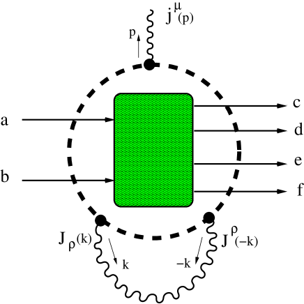
Figure 5: Example of one real and one virtual photon emissions. The electric current is a sum of contributions from all external particles. This is why it is attached to the dashed line which crosses all relevant external lines. The rest of the Feynman diagram is visualised as the internal dark box.

In order to introduce the notation, let us first write down explicitly the emission factor for a single-real photon

$$j^{\mu}(k)=ie\sum_{X=a,b,c,d,e,f}\!\!\!Q_{X}\theta_{X}\;\frac{2p_{X}^{\mu}}{2p_{X}k},$$ (C.1)

where $\theta_{X}=+1,-1$ for particles in the initial and final state, respectively, $Q_{X}$ is the charge of the particle (in the units of the positron charge $e$) and the single-virtual photon current reads

$$J^{\mu}(k)=\sum_{X=a,b,c,d,e,f}\hat{J}_{X}^{\mu}(k),\qquad\hat{J}_{X}^{\mu}(k)\equiv Q_{X}\theta_{X}\;\frac{2p_{X}^{\mu}\theta_{X}-k^{\mu}}{k^{2}-2p_{X}k\theta_{X}+i\varepsilon},$$ (C.2)

see fig. 5. For the virtual corrections we always have an even number of the $J^{\mu}(k)$ currents paired in the so-called virtual $S$-factor

$$S(k)=J(k)\circ J(k)=\sum_{{X=a,b,c,d,e,f}\atop{Y=a,b,c,d,e,f}}J_{X}(k)\circ J_{Y}(k),$$ (C.3)

where

$$J_{X}(k)\circ J_{Y}(k)=J_{X}(k)\cdot J_{Y}(-k),\;{\rm for}\;X\neq Y,\quad J_{X}(k)\circ J_{X}(k)=J_{X}(k)\cdot J_{X}(k).$$ (C.4)

In fig. 5 we illustrate all that in a visual way. The contribution $J_{X}(k)\cdot J_{X}(k)$ looks diagrammatically like the self-energy, but in fact it comes from the charge renormalisation, see the discussion in refs. [18, 52].

In the derivation of $\exp(\alpha B)$ of ref. [18] (taking as an example the four-fermion production process) we arrive at a certain stage where the contributions from all the real and virtual photons are factorised.

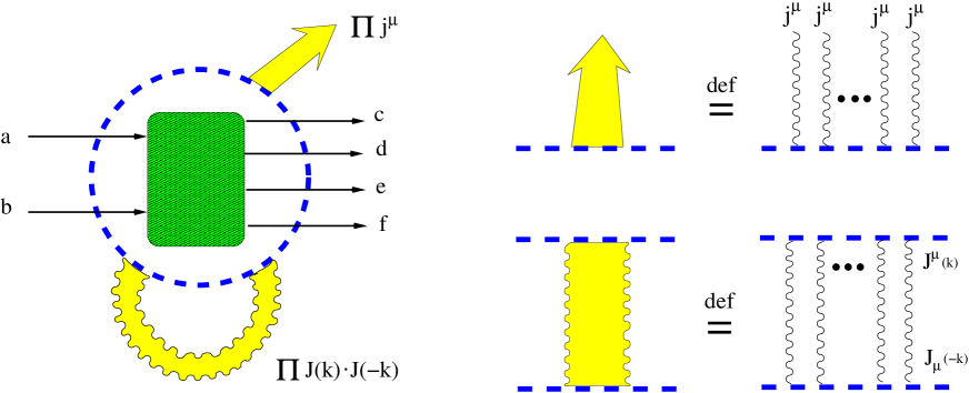
Figure 6: The EEX amplitude for four-fermion production. The electric current is a sum of contributions from all external particles. This is why it is attached to the dashed line which crosses all relevant external lines. We use the collective notation for multiple-photon lines which is defined in the plot.

The corresponding scattering amplitude with $m$ real and any number of virtual photons taken in the soft-photon approximation, visualised in fig. 6, reads

$$M^{\mu_{1}\mu_{2}...\mu_{m}}(k_{1},k_{2},...,k_{m})=$$ (C.5)

$$=\mathcal{M}\;\prod_{l=1}^{m}j^{\mu}(k_{l})\;\sum_{n=0}^{\infty}\frac{1}{n!}\prod_{i=1}^{n}\alpha\int\frac{i}{(2\pi)^{3}}\;\frac{d^{4}k_{i}}{k_{i}^{2}-\lambda^{2}+i\varepsilon}\;J^{\mu}(k_{i})\circ J_{\mu}(k_{i}).$$

The sum over virtual photons is done trivially, resulting in the exponential form-factor:

$$M^{\mu_{1}\mu_{2}...\mu_{m}}(k_{1},k_{2},...,k_{m})=\mathcal{M}\;\prod_{l=1}^{m}j^{\mu}(k_{l})\;e^{\alpha B_{6}},$$ (C.6)

$$B_{6}=\int\frac{i}{(2\pi)^{3}}\;\frac{d^{4}k}{k^{2}-\lambda^{2}+i\varepsilon}\;J(k)\circ J(k).$$

Note that in the residual function $\mathcal{M}$ there is no “recoil” dependence on photon momenta, we are therefore limited to very soft photons ($E_{\gamma}\ll\Gamma_{W}$) in the process of our interest.

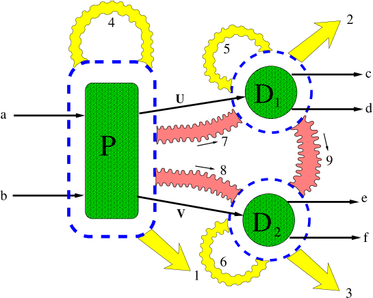
Figure 7: The CEEX amplitude for $WW$ production and two decays in the soft-photon approximation. Visualised are all classes of virtual and real photon emissions.

Let us now take into account the double-resonant character of the process, see fig. 7. After factorising all the real and virtual soft photons, and introducing a new source of emission from the intermediate resonant $W$’s, we use the identity of eq. (A.11) to arrive at the amplitude depicted in fig. 7, which can be written explicitly as follows:

$$M^{\mu_{{}_{1_{1}}}...\mu_{{}_{3_{n_{3}}}}}_{n_{1}n_{2}n_{3}}(k_{1_{1}},...,k_{3_{n_{3}}})=\mathcal{M}_{0}\;\prod_{i_{1}={1}}^{n_{1}}j^{\mu_{i_{1}}}_{P}(k_{i_{1}})\;\prod_{i_{2}={1}}^{n_{2}}j^{\mu_{i_{2}}}_{D_{1}}(k_{i_{2}})\;\prod_{i_{3}={1}}^{n_{3}}j^{\mu_{i_{3}}}_{D_{2}}(k_{i_{3}})\;$$ (C.7)

$$\quad\sum_{n_{4}=0}^{\infty}\frac{1}{n_{4}!}\prod_{i_{4}=1}^{n_{4}}\alpha\int\frac{i}{(2\pi)^{3}}\;\frac{d^{4}k_{i_{4}}}{k_{i_{4}}^{2}-m_{\gamma}^{2}+i\varepsilon}\;J_{P}(k_{i_{4}})\circ J_{P}(k_{i_{4}})\;$$

$$\quad\sum_{n_{5}=0}^{\infty}\frac{1}{n_{5}!}\prod_{i_{5}=1}^{n_{5}}\alpha\int\frac{i}{(2\pi)^{3}}\;\frac{d^{4}k_{i_{5}}}{k_{i_{5}}^{2}-m_{\gamma}^{2}+i\varepsilon}\;J_{D_{1}}(k_{i_{5}})\circ J_{D_{1}}(k_{i_{5}})$$

$$\quad\sum_{n_{6}=0}^{\infty}\frac{1}{n_{6}!}\prod_{i_{6}=1}^{n_{6}}\alpha\int\frac{i}{(2\pi)^{3}}\;\frac{d^{4}k_{i_{6}}}{k_{i_{6}}^{2}-m_{\gamma}^{2}+i\varepsilon}\;J_{D_{2}}(k_{i_{6}})\circ J_{D_{2}}(k_{i_{6}})$$

$$\quad\sum_{n_{7}=0}^{\infty}\frac{1}{n_{7}!}\prod_{i_{7}=1}^{n_{7}}2\alpha\int\frac{i}{(2\pi)^{3}}\;\frac{d^{4}k_{i_{7}}}{k_{i_{7}}^{2}-m_{\gamma}^{2}+i\varepsilon}\;J_{P}(k_{i_{7}})\circ J_{D_{1}}(k_{i_{7}})$$

$$\quad\sum_{n_{8}=0}^{\infty}\frac{1}{n_{8}!}\prod_{i_{8}=1}^{n_{8}}2\alpha\int\frac{i}{(2\pi)^{3}}\;\frac{d^{4}k_{i_{8}}}{k_{i_{8}}^{2}-m_{\gamma}^{2}+i\varepsilon}\;J_{P}(k_{i_{8}})\circ J_{D_{2}}(k_{i_{8}})$$

$$\quad\sum_{n_{9}=0}^{\infty}\frac{1}{n_{9}!}\prod_{i_{9}=1}^{n_{9}}2\alpha\int\frac{i}{(2\pi)^{3}}\;\frac{d^{4}k_{i_{9}}}{k_{i_{9}}^{2}-m_{\gamma}^{2}+i\varepsilon}\;J_{D_{1}}(k_{i_{9}})\circ J_{D_{2}}(k_{i_{9}})$$

$$\quad\frac{1}{(p_{cd}+K_{2}-K_{7}+K_{9})^{2}-M^{2}}\;\frac{1}{(p_{ef}+K_{3}-K_{8}-K_{9})-M^{2}},$$

where $K_{l}=\sum_{i_{l}=1}^{n_{l}}k_{i_{l}}$. We have defined nine groups of photons (labeled by $l$); $l=1,2,3$ corresponds, respectively, to the real emission from the $W$-pair production and their decays, the virtual photons corresponding to the same sources are denoted as the group (4,5,6), while (7,8) corresponds to the virtual photons attached to the production and the decay. Finally, the virtual photons denoted as the group (9) connect the decays of the first and the second $W$-boson.

The most interesting part in the above expression is that the product of two resonance propagators includes all the relevant recoil dependence on the real and virtual photon momenta. This dependence can be read easily from fig. 7. We are now not limited by $E_{\gamma}\ll\Gamma_{W}$, but rather by $E_{\gamma}\ll\sqrt{s}$. One important feature is that propagators do not depend on $K_{4}$, $K_{5}$ and $K_{6}$ – this is why the sums over relevant photons can be immediately folded into three standard YFS form-factor $e^{\alpha B}$, for the production and decay processes. This, however, cannot be done for the three virtual-interference contributions because the propagators do depend on $K_{7}$, $K_{8}$ and $K_{9}$. The dependence on the real photons $K_{2}$ and $K_{3}$ is not harmful for our task of summing up virtual contributions to the infinite order:

$$M^{\mu_{{}_{1_{1}}}...\mu_{{}_{3_{n_{3}}}}}_{n_{1}n_{2}n_{3}}(k_{1_{1}},...,k_{3_{n_{3}}})=\mathcal{M}_{0}\;\prod_{i_{1}={1}}^{n_{1}}j^{\mu_{i_{1}}}_{P}(k_{i_{1}})\;\prod_{i_{2}={1}}^{n_{2}}j^{\mu_{i_{2}}}_{D_{1}}(k_{i_{2}})\;\prod_{i_{3}={1}}^{n_{3}}j^{\mu_{i_{3}}}_{D_{2}}(k_{i_{3}})\;$$ (C.8)

$$\quad e^{\alpha B_{P}}\;e^{\alpha B_{D_{1}}}\;e^{\alpha B_{D_{2}}}\;\sum_{n_{7}=0}^{\infty}\frac{1}{n_{7}!}\prod_{i_{7}=1}^{n_{7}}2\alpha\int\frac{i}{(2\pi)^{3}}\;\frac{d^{4}k_{i_{7}}}{k_{i_{7}}^{2}-m_{\gamma}^{2}}\;J_{P}(k_{i_{7}})\circ J_{D_{1}}(k_{i_{7}})\;$$

$$\quad\sum_{n_{8}=0}^{\infty}\frac{1}{n_{8}!}\prod_{i_{8}=1}^{n_{8}}2\alpha\int\frac{i}{(2\pi)^{3}}\;\frac{d^{4}k_{i_{8}}}{k_{i_{8}}^{2}-m_{\gamma}^{2}}\;J_{P}(k_{i_{8}})\circ J_{D_{2}}(k_{i_{8}})$$

$$\quad\sum_{n_{9}=0}^{\infty}\frac{1}{n_{9}!}\prod_{i_{9}=1}^{n_{9}}2\alpha\int\frac{i}{(2\pi)^{3}}\;\frac{d^{4}k_{i_{9}}}{k_{i_{9}}^{2}-m_{\gamma}^{2}}\;J_{D_{1}}(k_{i_{9}})\circ J_{D_{2}}(k_{i_{9}})$$

$$\quad\frac{1}{(U_{2}-K_{7}+K_{9})^{2}-M^{2}}\;\frac{1}{(V_{3}-K_{8}-K_{9})-M^{2}},$$

where $U_{2}=p_{cd}+K_{2}$ and $V_{3}=p_{ef}+K_{3}$, and

$$\alpha B_{X}=\int\frac{i}{(2\pi)^{3}}\;\frac{d^{4}k}{k^{2}-m_{\gamma}^{2}+i\varepsilon}\;J_{X}(k)\circ J_{X}(k),\quad X=P,D_{1},D_{2}.$$ (C.9)

At this point we use the following approximations (valid in the soft-photon limit):

$$\frac{1}{(U_{2}-K_{7}+K_{9})^{2}-M^{2}}\;\simeq\frac{1}{U_{2}^{2}-M^{2}-2U_{2}K_{7}+2U_{2}K_{9}}\;$$ (C.10)

$$\quad=\frac{1}{U_{2}^{2}-M^{2}}\;\frac{1}{1-\sum_{i_{7}}\frac{2U_{2}k_{i_{7}}}{U_{2}^{2}-M^{2}}+\sum_{i_{9}}\frac{2U_{2}k_{i_{9}}}{U_{2}^{2}-M^{2}}}\;$$

$$\quad\simeq\frac{1}{U_{2}^{2}-M^{2}}\;\prod_{i_{7}}\frac{1}{1-\frac{2U_{2}k_{i_{7}}}{U_{2}^{2}-M^{2}}}\;\prod_{i_{9}}\frac{1}{1+\frac{2U_{2}k_{i_{9}}}{U_{2}^{2}-M^{2}}}\;$$

$$\quad\simeq\frac{1}{U_{2}^{2}-M^{2}}\;\prod_{i_{7}}\frac{U_{2}^{2}-M^{2}}{(U_{2}-k_{i_{7}})^{2}-M^{2}}\;\prod_{i_{9}}\frac{U_{2}^{2}-M^{2}}{(U_{2}+k_{i_{9}})^{2}-M^{2}}\;,$$

which, together with the analogous approximation for the second propagator, allows us to fold-in three remaining sums into exponents:

$$M^{\mu_{{}_{1_{1}}}...\mu_{{}_{3_{n_{3}}}}}_{n_{1}n_{2}n_{3}}(k_{1_{1}},...,k_{3_{n_{3}}})=\mathcal{M}_{0}\;\prod_{i_{1}={1_{1}}}^{n_{1}}j^{\mu_{i_{1}}}_{P}(k_{i_{1}})\;\prod_{i_{2}={1_{2}}}^{n_{2}}j^{\mu_{i_{2}}}_{D_{1}}(k_{i_{2}})\;\prod_{i_{3}={1_{3}}}^{n_{3}}j^{\mu_{i_{3}}}_{D_{2}}(k_{i_{3}})\;$$ (C.11)

$$\qquad\qquad e^{\alpha B_{10}^{\rm CEEX}(p_{cd}+K_{2},p_{ef}+K_{3})}\;\frac{1}{(p_{cd}+K_{2})^{2}-M^{2}}\;\frac{1}{(p_{ef}+K_{3})-M^{2}},$$

where

$$\alpha B_{10}^{\rm CEEX}(U,V)=\alpha B_{P}+\alpha B_{D_{1}}+\alpha B_{D_{2}}+2\alpha B_{P\otimes D_{1}}(U)+2\alpha B_{P\otimes D_{2}}(V)+2\alpha B_{D_{1}\otimes D_{2}}(U,V),\;$$ (C.12)

$$\alpha B_{P\otimes D_{1}}(U)=\int\frac{i}{(2\pi)^{3}}\;\frac{d^{4}k}{k^{2}-m_{\gamma}^{2}+i\varepsilon}\;J_{P}(k)\circ J_{D_{1}}(k)\frac{U^{2}-M^{2}}{(U-k)^{2}-M^{2}},$$

$$\alpha B_{P\otimes D_{2}}(V)=\int\frac{i}{(2\pi)^{3}}\;\frac{d^{4}k}{k^{2}-m_{\gamma}^{2}+i\varepsilon}\;J_{P}(k)\circ J_{D_{2}}(k)\frac{V^{2}-M^{2}}{(V-k)^{2}-M^{2}},$$

$$\alpha B_{D_{1}\otimes D_{2}}(U,V)=\int\frac{i}{(2\pi)^{3}}\;\frac{d^{4}k}{k^{2}-m_{\gamma}^{2}+i\varepsilon}\;J_{D_{1}}(k)\circ J_{D_{2}}(k)\frac{U^{2}-M^{2}}{(U+k)^{2}-M^{2}}\;\frac{V^{2}-M^{2}}{(V-k)^{2}-M^{2}}.$$

Let us note that in the no-recoil limit $U-k\to U$, $V-k\to V$, i.e. $k\ll\Gamma_{W}$, the function $B_{10}^{\rm CEEX}(U,V)$ reduces to $B_{6}^{\rm CEEX}$, in an analogous way to eq. (3.7).

In eq. (C.11) and in all previous steps the contributions of real photon were taken as just one term (in which we know to which subprocess every real photon belongs) from the grand sum (as defined e.g. in eq. (4.14)), over all $3^{n}$ photon assignments $(P,D_{1},D_{2})^{n}$, in which we know to which subprocess every real photon belongs. Let us restore this coherent sum over all photon assignments in the following compact final expression:

$$M^{\mu_{1}...\mu_{n}}(k_{1},k_{2},...,k_{n})=\!\!\!\!\!\sum_{\wp\in(P,D_{1},D_{2})^{n}}\!\!\!\!\mathcal{M}_{0}\;\prod_{i=1}^{n}j^{\mu_{i}}_{\wp_{i}}(k_{i})\;e^{\alpha B_{10}^{\rm CEEX}(U_{\wp},V_{\wp})}\;\frac{1}{U_{\wp}^{2}-M^{2}}\;\frac{1}{V_{\wp}^{2}-M^{2}},$$ (C.13)

where $U_{\wp}=p_{cd}+\sum\limits_{\wp_{i}=D_{1}}k_{i}$ and $V_{\wp}=p_{ef}+\sum\limits_{\wp_{i}=D_{2}}k_{i}$.

Eq. (C.13) is the principal result of this Appendix. The CEEX form-factor of eq. (C.13) is valid for production of a pair of any charged resonances of any spin. The case of a single charged resonance, or more than two charged resonances, can be treated in the same way.

The presented derivation of the virtual form-factor is based to a large extent on the analogy with the real-emission part (see Appendix B) and the cancellation between the real and virtual emissions.

References

• [1] J. Alcaraz, et al., Precision Electroweak Measurements and Constraints on the Standard Model (2007). arXiv:0712.0929.
• [2] S. Schael, et al., Electroweak Measurements in Electron-Positron Collisions at W-Boson-Pair Energies at LEP, Phys. Rept. 532 (2013) 119–244 (2013). arXiv:1302.3415, doi:10.1016/j.physrep.2013.07.004.
• [3] A. Abada, et al., FCC Physics Opportunities, Eur. Phys. J. C79 (6) (2019) 474 (2019). doi:10.1140/epjc/s10052-019-6904-3.
• [4] A. Abada, et al., FCC-ee: The Lepton Collider, Eur. Phys. J. ST 228 (2) (2019) 261–623 (2019). doi:10.1140/epjst/e2019-900045-4.
• [5] A. Blondel, et al., Standard Model Theory for the FCC-ee: The Tera-Z, in: Mini Workshop on Precision EW and QCD Calculations for the FCC Studies: Methods and Techniques CERN, Geneva, Switzerland, January 12-13, 2018, 2018 (2018). arXiv:1809.01830.
• [6] A. Blondel, A. Freitas, J. Gluza, S. Heinemeyer, S. Jadach, P. Janot, T. Riemann, Theory Requirements and Possibilities for the FCC-ee and other Future High Energy and Precision Frontier Lepton Colliders (2019). arXiv:1901.02648.
• [7] M. W. Grunewald, et al., Reports of the Working Groups on Precision Calculations for LEP2 Physics: Proceedings. Four fermion production in electron positron collisions (2000). arXiv:hep-ph/0005309.
• [8] W. Placzek, Precision predictions for W pair production at LEP-2 (2002) 172–176[Nucl. Phys. Proc. Suppl.117,172(2003)] (2002). arXiv:hep-ph/0208138, doi:10.1016/S0920-5632(03)90518-4.
• [9] S. Jadach, W. Placzek, M. Skrzypek, B. F. L. Ward, Z. Was, The Monte Carlo program KoralW version 1.51 and the concurrent Monte Carlo KoralW and YFSWW3 with all background graphs and first order corrections to W pair production, Comput. Phys. Commun. 140 (2001) 475–512 (2001). arXiv:hep-ph/0104049, doi:10.1016/S0010-4655(01)00296-X.
• [10] S. Jadach, W. Placzek, M. Skrzypek, B. F. L. Ward, Z. Was, Precision predictions for (un)stable W+ W- pair production at and beyond LEP-2 energies, Phys. Rev. D65 (2002) 093010 (2002). arXiv:hep-ph/0007012, doi:10.1103/PhysRevD.65.093010.
• [11] S. Jadach, W. Placzek, M. Skrzypek, B. F. L. Ward, Z. Was, Exact O (alpha) gauge invariant YFS exponentiated Monte Carlo for (un)stable $W^{+}W^{-}$ production at and beyond LEP-2 energies, Phys. Lett. B417 (1998) 326–336 (1998). arXiv:hep-ph/9705429, doi:10.1016/S0370-2693(97)01253-7.
• [12] S. Jadach, W. Płaczek, M. Skrzypek, B. F. L. Ward, Z. Wa̧s, The Monte Carlo event generator YFSWW3 version 1.16 for W pair production and decay at LEP2/LC energies, Comput. Phys. Commun. 140 (2001) 432–474 (2001). arXiv:hep-ph/0103163, doi:10.1016/S0010-4655(01)00288-0.
• [13] J. Fleischer, F. Jegerlehner, M. Zralek, Radiative Corrections to Helicity Amplitudes for W Pair Production in $e^{+}e^{-}$ Annihilation, Z. Phys. C42 (1989) 409 (1989). doi:10.1007/BF01548446.
• [14] K. Kolodziej, M. Zralek, Helicity amplitudes for spin 0 or spin 1 boson production in $e^{+}e^{-}$ annihilation, Phys. Rev. D43 (1991) 3619–3625 (1991). doi:10.1103/PhysRevD.43.3619.
• [15] J. Fleischer, K. Kolodziej, F. Jegerlehner, W pair production in $e^{+}e^{-}$ annihilation: Radiative corrections including hard bremsstrahlung, Phys. Rev. D47 (1993) 830–836 (1993). doi:10.1103/PhysRevD.47.830.
• [16] J. Fleischer, F. Jegerlehner, K. Kolodziej, G. J. van Oldenborgh, EEWW: A generator for $e^{+}e^{-}\to W^{+}W^{-}$ including one loop and leading photonic two loop corrections, Comput. Phys. Commun. 85 (1995) 29–39 (1995). arXiv:hep-ph/9405380, doi:10.1016/0010-4655(94)00113-G.
• [17] S. Jadach, W. Placzek, M. Skrzypek, B. F. L. Ward, Z. Was, Monte Carlo program KoralW 1.42 for all four-fermion final states in $e^{+}e^{-}$ collisions, Comput. Phys. Commun. 119 (1999) 272–311 (1999). arXiv:hep-ph/9906277, doi:10.1016/S0010-4655(99)00219-2.
• [18] D. R. Yennie, S. C. Frautschi, H. Suura, The infrared divergence phenomena and high-energy processes, Annals Phys. 13 (1961) 379–452 (1961). doi:10.1016/0003-4916(61)90151-8.
• [19] S. Jadach, Z. Was, R. Decker, J. H. Kuhn, The tau decay library TAUOLA: Version 2.4, Comput. Phys. Commun. 76 (1993) 361–380 (1993). doi:10.1016/0010-4655(93)90061-G.
• [20] E. Barberio, B. van Eijk, Z. Was, PHOTOS: A Universal Monte Carlo for QED radiative corrections in decays, Comput. Phys. Commun. 66 (1991) 115–128 (1991). doi:10.1016/0010-4655(91)90012-A.
• [21] A. Denner, S. Dittmaier, M. Roth, D. Wackeroth, Electroweak radiative corrections to e+ e- $\to$ W W $\to$ 4 fermions in double pole approximation: The RACOONWW approach, Nucl. Phys. B587 (2000) 67–117 (2000). arXiv:hep-ph/0006307, doi:10.1016/S0550-3213(00)00511-3.
• [22] A. Denner, S. Dittmaier, M. Roth, D. Wackeroth, RACOONWW1.3: A Monte Carlo program for four fermion production at $e^{+}e^{-}$ colliders, Comput. Phys. Commun. 153 (2003) 462–507 (2003). arXiv:hep-ph/0209330, doi:10.1016/S0010-4655(03)00205-4.
• [23] S. Jadach, M. Skrzypek, QED challenges at FCC-ee precision measurements, Eur. Phys. J. C79 (9) (2019) 756 (2019). arXiv:1903.09895, doi:10.1140/epjc/s10052-019-7255-9.
• [24] S. Jadach, B. F. L. Ward, Z. Was, The Precision Monte Carlo event generator KK for two fermion final states in $e^{+}e^{-}$ collisions, Comput. Phys. Commun. 130 (2000) 260–325 (2000). arXiv:hep-ph/9912214, doi:10.1016/S0010-4655(00)00048-5.
• [25] S. Jadach, B. F. L. Ward, Z. Was, Coherent exclusive exponentiation for precision Monte Carlo calculations, Phys. Rev. D63 (2001) 113009 (2001). arXiv:hep-ph/0006359, doi:10.1103/PhysRevD.63.113009.
• [26] S. Jadach, B. F. L. Ward, YFS2: The Second Order Monte Carlo for Fermion Pair Production at LEP / SLC With the Initial State Radiation of Two Hard and Multiple Soft Photons, Comput. Phys. Commun. 56 (1990) 351–384 (1990). doi:10.1016/0010-4655(90)90020-2.
• [27] S. Jadach, B. F. L. Ward, Final state multiple photon effects in fermion pair production at SLC / LEP, Phys. Lett. B274 (1992) 470–472 (1992). doi:10.1016/0370-2693(92)92017-B.
• [28] S. Jadach, Z. Was, Monte Carlo Simulation of the Process e+ e- —¿ tau+ tau- Including Radiative O(alpha**3) QED Corrections, Mass and Spin, Comput. Phys. Commun. 36 (1985) 191–211 (1985). doi:10.1016/0010-4655(85)90123-7.
• [29] S. Jadach, B. F. L. Ward, Z. Was, The Monte Carlo program KORALZ, version 3.8, for the lepton or quark pair production at LEP / SLC energies, Comput. Phys. Commun. 66 (1991) 276–292 (1991). doi:10.1016/0010-4655(91)90077-X.
• [30] W. Placzek, S. Jadach, Multiphoton radiation in leptonic W boson decays, Eur. Phys. J. C29 (2003) 325–339 (2003). arXiv:hep-ph/0302065, doi:10.1140/epjc/s2003-01223-4.
• [31] A. Denner, S. Dittmaier, M. Roth, L. H. Wieders, Complete electroweak O(alpha) corrections to charged-current $e^{+}e^{-}\to$ 4 fermion processes, Phys. Lett. B612 (2005) 223–232, [Erratum: Phys. Lett.B704,667(2011)] (2005). arXiv:hep-ph/0502063, doi:10.1016/j.physletb.2005.03.007.
• [32] A. Denner, S. Dittmaier, M. Roth, L. H. Wieders, Electroweak corrections to charged-current $e^{+}e^{-}\to$ 4 fermion processes: Technical details and further results, Nucl. Phys. B724 (2005) 247–294, [Erratum: Nucl. Phys.B854,504(2012)] (2005). arXiv:hep-ph/0505042, doi:10.1016/j.nuclphysb.2005.06.033.
• [33] M. Beneke, P. Falgari, C. Schwinn, A. Signer, G. Zanderighi, Four-fermion production near the W pair production threshold, Nucl. Phys. B792 (2008) 89–135 (2008). arXiv:0707.0773, doi:10.1016/j.nuclphysb.2007.09.030.
• [34] S. Actis, M. Beneke, P. Falgari, C. Schwinn, Dominant NNLO corrections to four-fermion production near the W-pair production threshold, Nucl. Phys. B807 (2009) 1–32 (2009). arXiv:0807.0102, doi:10.1016/j.nuclphysb.2008.08.006.
• [35] S. Jadach, W. Płaczek, M. Skrzypek, Exponentiation in QED and Quasi-Stable Charged Particles, Symmetry 11 (11) (2019) 1389 (2019). doi:10.3390/sym11111389.
• [36] R. G. Stuart, Production cross-sections for unstable particles, Nucl. Phys. B498 (1997) 28–38 (1997). arXiv:hep-ph/9504215, doi:10.1016/S0550-3213(97)00276-9.
• [37] S. Jadach, W. Placzek, M. Skrzypek, B. F. L. Ward, Z. Was, On theoretical uncertainties of the W boson mass measurement at LEP-2, Phys. Lett. B523 (2001) 117–126 (2001). arXiv:hep-ph/0109072, doi:10.1016/S0370-2693(01)01310-7.
• [38] W. Beenakker, A. Denner, Standard model predictions for $W$ pair production in electron - positron collisions, Int. J. Mod. Phys. A9 (1994) 4837–4920 (1994). doi:10.1142/S0217751X94001965.
• [39] A. P. Chapovsky, V. A. Khoze, Screened Coulomb ansatz for the nonfactorizable radiative corrections to the off-shell W+ W- production, Eur. Phys. J. C9 (1999) 449–457 (1999). arXiv:hep-ph/9902343, doi:10.1007/s100529900070.
• [40] S. Jadach, B. F. L. Ward, Exponentiation of Soft Photons in the Monte Carlo: The Case of Bonneau and Martin, Phys. Rev. D38 (1988) 2897, [Erratum: Phys. Rev.D39,1471(1989)] (1988). doi:10.1103/PhysRevD.39.1471.2.
• [41] S. Jadach, B. F. L. Ward, Z. Was, Coherent exclusive exponentiation CEEX: The Case of the resonant $e^{+}e^{-}$ collision, Phys. Lett. B449 (1999) 97–108 (1999). arXiv:hep-ph/9905453, doi:10.1016/S0370-2693(99)00038-6.
• [42] S. Jadach, B. F. L. Ward, Multi - Photon Monte Carlo for Bhabha Scattering at Low Angles, Phys. Rev. D40 (1989) 3582–3589 (1989). doi:10.1103/PhysRevD.40.3582.
• [43] S. Jadach, B. F. L. Ward, Z. Was, The Monte Carlo program KORALZ, version 4.0, for the lepton or quark pair production at LEP / SLC energies, Comput. Phys. Commun. 79 (1994) 503–522 (1994). doi:10.1016/0010-4655(94)90190-2.
• [44] S. Jadach, E. Richter-Was, B. F. L. Ward, Z. Was, Monte Carlo program BHLUMI-2.01 for Bhabha scattering at low angles with Yennie-Frautschi-Suura exponentiation, Comput. Phys. Commun. 70 (1992) 305–344 (1992). doi:10.1016/0010-4655(92)90196-6.
• [45] S. Jadach, W. Placzek, E. Richter-Was, B. F. L. Ward, Z. Was, Upgrade of the Monte Carlo program BHLUMI for Bhabha scattering at low angles to version 4.04, Comput. Phys. Commun. 102 (1997) 229–251 (1997). doi:10.1016/S0010-4655(96)00156-7.
• [46] S. Jadach, B. F. L. Ward, Z. A. Was, S. A. Yost, Systematic Studies of Exact ${\cal O}(\alpha^{2}L)$ CEEX EW Corrections in a Hadronic MC for Precision $Z/\gamma^{*}$ Physics at LHC Energies (2017). arXiv:1707.06502.
• [47] S. Jadach, W. Placzek, B. F. L. Ward, BHWIDE 1.00: O(alpha) YFS exponentiated Monte Carlo for Bhabha scattering at wide angles for LEP-1 / SLC and LEP-2, Phys. Lett. B390 (1997) 298–308, also hep-ph/9608412; The Monte Carlo program BHWIDE is available from http://cern.ch/placzek (1997). arXiv:hep-ph/9608412, doi:10.1016/S0370-2693(96)01382-2.
• [48] M. Greco, G. Pancheri-Srivastava, Y. Srivastava, Radiative Corrections for Colliding Beam Resonances, Nucl. Phys. B101 (1975) 234–262 (1975). doi:10.1016/0550-3213(75)90304-1.
• [49] M. Greco, G. Pancheri-Srivastava, Y. Srivastava, Radiative Corrections to $e^{+}e^{-}\to\mu^{+}\mu^{-}$ Around the Z0, Nucl. Phys. B171 (1980) 118, [Erratum: Nucl. Phys. B197,543(1982)] (1980). doi:10.1016/0550-3213(80)90363-6.
• [50] V. S. Fadin, V. A. Khoze, A. D. Martin, Interference radiative phenomena in the production of heavy unstable particles, Phys. Rev. D49 (1994) 2247–2256 (1994). doi:10.1103/PhysRevD.49.2247.
• [51] S. Dittmaier, A General approach to photon radiation off fermions, Nucl. Phys. B565 (2000) 69–122 (2000). arXiv:hep-ph/9904440, doi:10.1016/S0550-3213(99)00563-5.
• [52] S. Weinberg, The Quantum Theory of Fields, The Press Syndicate of the University of Cambridge, 1995 (1995).