On the different forms of the kinematical constraint in BFKL

Abstract

We perform a detailed analysis of the different forms of the kinematical constraint imposed on the low $x$ evolution that appear in the literature. We find that all of them generate the same leading anti-collinear poles in Mellin space which agree with BFKL up to NLL order and up to NNLL in $N=4$ sYM. The coefficients of subleading poles vanish up to NNLL order for all constraints and we prove that this property should be satisfied to all orders. We then demonstrate that the kinematical constraints differ at further subleading orders of poles. We quantify the differences between the different forms of the constraints by performing numerical analysis both in Mellin space and in momentum space. It can be shown that in all three cases BFKL equation can be recast into the differential form, with the argument of the longitudinal variable shifted by the combination of the transverse coordinates.

1 Introduction

The sharp increase of the structure function $F_{2}$ in Deep Inelastic Scattering process with decreasing value of Bjorken variable $x$ was one of the biggest discoveries at HERA collider [1, 2]. This rise of $F_{2}$ is being driven in QCD by the increase in the gluon density due to dominance of gluon splitting when the parton’s longitudinal momentum fraction is small. Understanding the behavior of the parton densities at small $x$ is not only crucial for the DIS processes but also for the high energy hadronic collisions in accelerators and in the cosmic ray interactions. The LHC opened up the kinematic regime which is particularly sensitive to small $x$ values and thus the region where the gluon density dominates. The increase of the gluon density towards small $x$ translates then into the rise of the hadronic cross sections for variety of observables with the increasing center-of-mass energy. Within the framework of collinear factorization [3] the evolution of the gluon density is governed by the DGLAP [4, 5, 6] evolution equations which lead to the scaling violations. Although the DIS data are well described by the fits based on the DGLAP evolution, there are hints of novel physics phenomena that can be present at very small values of $x$ [7]. The alternative approach to the description of the parton evolution stems from the analysis of the Regge limit in QCD, where the energy of the interaction is assumed to be large $s\rightarrow\infty$, or in the case of the DIS process, when $x\rightarrow 0$, while the scale $Q^{2}$ is perturbative but fixed. In this limit the cross section is dominated by the exchange of the so-called hard Pomeron which is the solution to the famous BFKL evolution equation [8, 9, 10], see [11] for a review. The two notable differences between DGLAP and BFKL evolution equations are that in the latter the solution exhibits the power like behaviour, $x^{-\lambda}$ at small values of $x$ and the transverse momenta in the gluon cascade are not ordered. The solution thus depends on the transverse momenta of the exchanged reggeized gluons. BFKL equation is known up to NLL order in QCD [12, 13] and up to NNLL order in $N=4$ sYM theory [14, 15, 16]. A known issue with the BFKL at the NLL order is that the corrections are large compared to the LL result, which renders the result unstable. Thus it was early realized that higher order corrections need to be resummed. In the pioneering works [17, 18, 19] it was pointed out that there are kinematical constraints which need to be included in the evolution. Formally of higher order, when viewed from the perspective of the Regge limit, nevertheless such corrections are numerically very large as was established in [19]. Kinematical constraint was later included in the formalism that combined DGLAP and BFKL equations, and it was demonstrated that very good description of the HERA data was obtained [20]. Various elaborated resummation schemes for the small $x$ evolution were later developed [21, 22, 23, 24, 25, 26, 27, 28, 29, 30, 31, 32, 33, 34, 35]. More recently the collinear resummation was applied to the non-linear evolution equations in transverse coordinate space [36, 37, 38, 39].

Given the increased precision of the experimental data and progress in theoretical computations, especially the information about the higher orders in $N=4$ sYM theory, it is worth to revisit the assumptions in the resummed schemes. Even though the kinematical constraint is well motivated, different approximations, which are used are usually done based on general grounds (i.e. for example low $z$ approximation) but without detailed quantitative analysis. The differences between different forms of constraints may be of subleading order but it could happen that they are quite large numerically. In context of the BFKL equation, which utilizes the kinematical constraint as an ingredient, usually one uses a particular form of this constraint, namely the one which limits the transverse momenta of the exchanged gluons. Such choice is also dictated by practical applications, since in this form the angular variable in the evolution equation is integrated over which reduces the number of variables and makes it easier to solve the equation. On the other hand, there are different forms of the kinematical constraint that appear in the literature, which put limit on the transverse momenta of the emitted gluons. Actually in the CCFM equation which receives contribution from both large and low $x$ it is a natural choice [40].

The main goal of this paper is to perform a systematic semi-analytic and numerical comparison of the small $x$ evolution equation with different forms of the kinematical constraint, which appear in the literature.

In the analysis performed in this work we found that the constrains all generate the same structure in the Mellin space for the leading and first subleading anti-collinear poles up to NLL order in $\ln 1/x$ in QCD and in $N=4$ sYM and up to NNLL in $N=4$ sYM. As such they are all consistent up to the highest known order of perturbation theory. The calculations were performed both in the Mellin space and also by performing the direct solution of the BFKL with kinematical constraint in the momentum space. To this aim we have developed new numerical method for the solution of the BFKL equation with kinematical constraint which is based on reformulating this equation in the differential form. It turns out that all the constraints can be recast as effective shift of the longitudinal momentum fraction in the argument of the unintegrated gluon distribution. We see that, as expected the solutions are substantially reduced with respect to the LL case, but the differences between the different forms of the kinematical constraints are non-negligible and can reach up to 10-15 % for the value of the intercept. This can have important effect for the phenomenology.

2 Kinematical constraints

In this section we shall review the origin and different forms of the kinematical constraints that appear in the literature. The kinematical constraint in the initial state cascade at low $x$ was first considered in works [17, 41, 18].

We shall follow here closely the derivation presented in [19], where the kinematical constraint was implemented both in BFKL and the CCFM equations [17, 41, 42, 43, 44]. The latter evolution equation is based on the idea of coherence [45] that leads to the angular ordering of the emissions in the cascade. The BFKL equation for the unintegrated gluon density in the leading logarithmic approximation [10, 9, 8] can be written as

$${\cal F}(x,{k}_{\scaleto{T}{4pt}}^{2})={\cal F}^{(0)}(x,{k}_{\scaleto{T}{4pt}}^{2})\\ +\bar{\alpha}_{s}\int_{x}^{1}\frac{dz}{z}\int\frac{d^{2}{\bf q}_{\scaleto{T}{4pt}}}{\pi{q}_{\scaleto{T}{4pt}}^{2}}\left[{\cal F}\left(\frac{x}{z},\left|{\bf k}_{\scaleto{T}{4pt}}+{\bf q}_{\scaleto{T}{4pt}}\right|^{2}\right)-\Theta({k}_{\scaleto{T}{4pt}}^{2}-{q}_{\scaleto{T}{4pt}}^{2}){\cal F}\left(\frac{x}{z},{k}_{\scaleto{T}{4pt}}^{2}\right)\right]\;,$$ (1)

where function ${\cal F}(x,{k}_{\scaleto{T}{4pt}}^{2})$ is the small $x$ unintegrated gluon density, ${\bf k}_{\scaleto{T}{4pt}}$ and ${\bf k}_{\scaleto{T}{4pt}}^{\prime}={\bf k}_{\scaleto{T}{4pt}}+{\bf q}_{\scaleto{T}{4pt}}$ are the transverse momenta of the exchanged gluons and ${\bf q}_{\scaleto{T}{4pt}}$ is the transverse momentum of the gluon emitted. The longitudinal momentum fractions of the exchanged gluons are $x$ and ${x\over z}$ respectively. The flow of the momenta in the BFKL cascade is illustrated in diagram Fig. 1.

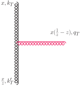
Figure 1: Schematic diagram representing gluon emission in the BFKL chain. $x$ and $x/z$ are the longitudinal momentum fractions of the target’s momentum carried by the exchanged gluon. ${\bf k}_{\scaleto{T}{4pt}},{\bf k}_{\scaleto{T}{4pt}}^{\prime}$ and ${\bf q}_{\scaleto{T}{4pt}}$ denote the two-dimensional transverse momenta of the exchanged gluons and the emitted gluon respectively.

We will also use the notation ${k}_{\scaleto{T}{4pt}}^{2}\equiv{\bf k}_{\scaleto{T}{4pt}}^{2}$ for the squared transverse momenta for the rest of the paper. The rescaled coupling constant is defined as $\bar{\alpha}_{s}\equiv\frac{\alpha_{s}N_{c}}{\pi}$. In the leading logarithmic approximation the integration over ${{\bf q}_{\scaleto{T}{4pt}}}$ in the Eq. (1), is not constrained by an upper limit thus violating the energy-momentum conservation. Thus for example in the context of the DIS process in principle there should be a limit on the integration over the transverse momentum

$$Q^{2}/x\sim W^{2}\,,$$ (2)

where $Q^{2}$ is the hard scale of the DIS process, $x$ is the Bjorken variable and $W^{2}$ is the c.m.s energy squared of the photon-proton system in DIS.

There is a stronger constraint arising however from the requirement that in the low $x$ formalism the exchanged gluons have off-shellness dominated by the transverse components, i.e. one keeps terms that obey $|k^{2}|\simeq{k}_{\scaleto{T}{4pt}}^{2}$. The derivation of the kinematical constraint here follows [19].

The gluon four momentum is as usual decomposed into light cone and transverse components

$$k=(k^{+},k^{-},{\bf k}_{\scaleto{T}{4pt}})\,,$$ (3)

where $k^{\pm}=k^{0}\pm k^{3}$. Now the exchanged gluon virtuality in these variables is equal to

$$k^{2}=k^{+}k^{-}-{k}_{\scaleto{T}{4pt}}^{2}\;.$$ (4)

The condition $|k^{2}|\simeq{k}_{\scaleto{T}{4pt}}^{2}$ translates approximately to

$${k}_{\scaleto{T}{4pt}}^{2}>k^{+}k^{-}\,.$$ (5)

The emitted gluon is on-shell $q^{2}=q^{+}q^{-}-{q}_{\scaleto{T}{4pt}}^{2}=0$, and therefore we can express this fact as

$$q^{-}={q}_{\scaleto{T}{4pt}}^{2}/q^{+}\,.$$ (6)

On the other hand in the multi-Regge kinematics there is a strong ordering of longitudinal momenta so

$$k^{-}=k^{{}^{\prime}-}-q^{-}\simeq q^{-}\,.$$ (7)

Using the condition (6) and inserting it into (5) one finally obtains

$${k}_{\scaleto{T}{4pt}}^{2}>k^{+}\frac{{q}_{\scaleto{T}{4pt}}^{2}}{q^{+}}=\frac{z}{1-z}{q}_{\scaleto{T}{4pt}}^{2}\;,$$ (8)

or as limit on ${q}_{\scaleto{T}{4pt}}^{2}$ integration

$${q}_{\scaleto{T}{4pt}}^{2}<\frac{1-z}{z}{k}_{\scaleto{T}{4pt}}^{2}\;.$$ (9)

Now there are several approximations that can be made to this constraint. In the small $z$ limit  (9) can be approximated to

$${q}_{\scaleto{T}{4pt}}^{2}<\frac{{k}_{\scaleto{T}{4pt}}^{2}}{z}\,.$$ (10)

This form of the approximation was used in [17] and also studied in the context of small $x$ approximation to the CCFM evolution in [19]. The lower bound on $z$, i.e. $z>x$ results in the upper bound on ${q}_{\scaleto{T}{4pt}}^{2}<{k}_{\scaleto{T}{4pt}}^{2}/x$ providing local condition for energy-momentum conservation.

Finally, (9) can be further rewritten as a condition on the transverse momentum of the exchanged gluon ${k}_{\scaleto{T}{4pt}}^{\prime}$. For a given value of ${k}_{\scaleto{T}{4pt}}$ a high value of ${k}_{\scaleto{T}{4pt}}^{\prime}$ means also high value of ${q}_{\scaleto{T}{4pt}}$. Rewriting it as

$${k}_{\scaleto{T}{4pt}}^{\prime 2}-2{k}_{\scaleto{T}{4pt}}^{\prime}\cdot{k}_{\scaleto{T}{4pt}}+{k}_{\scaleto{T}{4pt}}^{2}<\frac{1-z}{z}{k}_{\scaleto{T}{4pt}}^{2}\,,$$ (11)

and averaging over angle between ${k}_{\scaleto{T}{4pt}}$ and ${k}_{\scaleto{T}{4pt}}^{\prime}$ and taking large ${k}_{\scaleto{T}{4pt}}^{\prime}$ limit we get:

$${k}_{\scaleto{T}{4pt}}^{\prime 2}<\frac{{k}_{\scaleto{T}{4pt}}^{2}}{z}\,.$$ (12)

This form of the constraint was used for example in [18] and in [20, 46, 29, 47, 48]. The nice feature of (12) is the fact that the kernel with kinematical constraint has a Mellin representation which results in a simple shift of poles in the Mellin space. In the rest of the paper we shall analyze in detail all the forms of the constraints and quantify the differences between them both in Mellin space and through direct numerical solution ot the BFKL equation in momentum space.

3 Comparison of improved kernel with results in $N=4$ sYM

Since the works of [18, 19] it is known that the kinematical constraint provides very important contribution to the NLL order and beyond in BFKL. Even though formally of subleading order, numerically this correction is very large and leads to the strong reduction of the intercept, aligning the BFKL equation more with phenomenology, for selected early works which implement kinematical corrections in BFKL see for example [20, 49, 50, 51]. At the NLL order the kinematical constraint, when viewed as a correction in the Mellin space gives rise to the cubic poles in the Mellin conjugated variable to the transverse momentum in the BFKL eigenvalue. The $N=4$ sYM eigenvalue at LL is identical to the QCD case, and at NLL the same leading cubic poles appear in both theories [52]. Since the constraint is originating from the kinematics specific to the Regge limit of the cascade, one could expect it to be universal in both theories. It is useful to explore whether or not the kinematical constraint correctly reproduces the terms in the higher order NNLL known only in the supersymmetric case [14, 15, 16] and what are the differences between the different forms of the kinematical constraint discussed in the literature.

In this section we shall perform a detailed comparison of leading and subleading poles in the Mellin space originating from the kinematical constraint with the results in $N=4$ sYM case up to NNLL. First, we shall perform the comparison on the example of the constraint (12). Later on, in Sec. 4, we shall check that the results are consistent for different forms of the kinematical constraints up to certain order of poles, and we shall identify this order. In that way we can quantify the level of differences between different forms of the constraints.

3.1 NLL and NNLL of N=4 sYM and $\omega$ expansion

Let us begin with recalling the definition of the BFKL eigenvalue and the Mellin transform.

The Mellin transformation into the $\omega$ space is defined as

$$\overline{\cal F}(\omega,k_{T}^{2})=\int_{0}^{1}\frac{dz}{z}z^{\omega}\,{\cal F}(z,{k}_{\scaleto{T}{4pt}}^{2})\;,$$ (13)

and into the $\gamma$ space as

$$\tilde{{\cal F}}(\omega,\gamma)=\int_{0}^{\infty}d{k}_{\scaleto{T}{4pt}}^{2}\left({k}_{\scaleto{T}{4pt}}^{\prime 2}\right)^{-\gamma}{\cal F}(\omega,{k}_{\scaleto{T}{4pt}}^{2})\;,$$ (14)

Applying it to the BFKL equation we get the algebraic form of the BFKL equation

$$\tilde{{\cal F}}(\omega,\gamma)=\tilde{{\cal F}}^{(0)}(\omega,\gamma)+\frac{\bar{\alpha}_{s}}{\omega}\chi(\gamma,\omega)\tilde{{\cal F}}(\omega,\gamma)\,,$$ (15)

where $\chi(\gamma,\omega)$ is the kernel transformed to the double Mellin space. The $\omega$ dependence stems from the $z$ dependence of the kernel $K$ due to the kinematical constraint. Of course the fixed order LL and NLL kernels do not have the $\omega$ dependence, it is only the resummed kernel, in this case the kernel with the kinematical constraint that obtains this additional dependence. As is well known, see for example [19, 20, 21, 46, 29], such dependence in turn generates the series in $\alpha_{s}$ and therefore resums the contributions from all orders in the strong coupling. The result with the constraint (12) is well known [18]

$$\chi(\gamma,\omega)=2\psi(1)-\psi(\gamma)-\psi(1-\gamma+\omega)\,.$$ (16)

where $\psi$ is a polygamma function. When $\omega=0$ the above result coincides with the LL BFKL eigenvalue in QCD and in N=4 sYM

$$\chi_{0}(\gamma)=2\psi(1)-\psi(\gamma)-\psi(1-\gamma)\,.$$ (17)

We shall investigate Mellin forms of the kernels with other constraints (9) and (10) later on in Sec.4. In order to compare the results with NLL and NNLL calculations one needs to specify the correct scale choice. The above result leads to an asymmetric kernel which is valid in the so-called asymmetric scale choice. That means it is valid when considering the DIS process, in which the $x$ Bjorken is defined as $x=Q^{2}/s$ with $Q^{2}$ the (minus) virtuality of the photon. For the case of the different process, like for example Mueller-Navelet jets with comparable transverse momenta, the appropriate variable would be $QQ_{0}/s$, where $Q\simeq Q_{0}$ are the scales of the order of transverse momenta of the jets. The eigenvalue in this case would be different from (16) as it should correspond to the symmetric choice of scales. Therefore one needs to perform the scale changing transformation which generates terms starting at an appropriate order. Up to NLL order this was discussed in [13, 12, 21]. We shall recall in detail the scale changing transformation, and what terms it generates up to NNLL in the next subsection, here we shall directly start from the symmetric counterpart of the eigenvalue (16) which has the following form

$$\chi(\gamma,\omega)=2\psi(1)-\psi(\gamma+\frac{\omega}{2})-\psi(1-\gamma+\frac{\omega}{2})\,.$$ (18)

The result for the NNLL eigenvalue in the case of the $N=4$ sYM was derived originally in [14, 15] for the symmetric case. It was later on rederived in [16] by exploiting the correspondence between the soft-gluon wide-angle radiation in jet physics and the BFKL physics. To have direct relation to these results we will focus below on the symmetric case. The poles around $\gamma=0$ of NLL [52] and NNLL kernel in N=4 sYM are given by [14, 15, 16]

$$\chi_{1}^{sYM}=-\frac{1}{2\gamma^{3}}-1.79+{\cal O}(\gamma)\;,$$ (19)

$$\chi_{2}^{sYM}=\frac{1}{2\gamma^{5}}-\frac{\zeta(2)}{\gamma^{3}}-\frac{9\zeta(3)}{4\gamma^{2}}-\frac{29\zeta(4)}{8\gamma}+{\cal O}(1)\;.$$ (20)

Since it is symmetric case the coefficients of the poles around $\gamma=0$ and $\gamma=1$ are identical. For the purpose of simplification therefore we only focus on the expansion around $\gamma=0$. We can retrieve the leading and the vanishing subleading poles of the $N=4$ sYM case by doing $\omega$ expansion of the shifted eigenvalue (18)

$$\chi(\gamma,\omega)=2\psi(1)-\psi(\gamma+\frac{\omega}{2})-\psi(1-\gamma+\frac{\omega}{2})=\chi_{0}+\chi^{(1)}\frac{\omega}{2}+\frac{1}{2!}\chi^{(2)}\left(\frac{\omega}{2}\right)^{2}+\dots\;,$$ (21)

where the $\chi^{(i)}$ is the i-th derivative of $\chi^{\omega}$ with respect to $\omega$. The term lowest in order in $\bar{\alpha}_{s}$ in the expansion is simply $\chi_{0}$ which is the LL eigenvalue (17). In order to retrieve the term contributing to the NLL order we use the solution to the equation for the intercept in the lowest order of the coupling, i.e. $\omega_{0}=\bar{\alpha}_{s}\chi_{0}$, and substitute it into (21) and keep terms up to first power in $\bar{\alpha}_{s}$. One obtains

$$\chi(\gamma)=\chi_{0}+\frac{1}{2}\bar{\alpha}_{s}\chi^{(1)}\chi_{0}\;.$$ (22)

This gives the contribution to the NLL order

$$\chi_{1}(\gamma)=\frac{1}{2}\chi^{(1)}\chi_{0}=\frac{1}{2}\left[\psi^{(1)}(\gamma)+\psi^{(1)}(1-\gamma)\right]\left[2\psi(1)-\psi(\gamma)-\psi(1-\gamma)\right]\,.$$ (23)

Expanding around $\gamma=0$ one obtains the following pole structure

$$\chi_{1}(\gamma)=-\frac{1}{2\gamma^{3}}-\frac{\zeta(2)}{\gamma}+O(1)\,.$$ (24)

Similarly, we can derive the term contributing at NNLL level from the $\omega$ expansion to the second order by taking $\omega_{1}=\bar{\alpha}_{s}\chi_{0}+\bar{\alpha}_{s}^{2}\chi_{1}$, substituting again into (21) and extracting terms proportional to $\bar{\alpha}_{s}^{2}$ which results in

$$\chi_{2}=\frac{1}{4}\left(\chi^{(1)}\right)^{2}\chi_{0}+\frac{1}{8}\chi^{(2)}\left(\chi_{0}\right)^{2}\;.$$ (25)

In this case the pole structure is

$$\chi_{2}=\frac{1}{2\gamma^{5}}+\frac{\zeta(2)}{\gamma^{3}}+\frac{2\zeta(3)}{\gamma^{2}}+O\left(\frac{1}{\gamma}\right)\;.$$ (26)

We observe that the leading poles $-1/2\gamma^{3}$ (24) and $1/2\gamma^{5}$ (26) coincide with the exact result at NLL in $N=4$ SYM and in QCD and NNLL order in $N=4$ SYM (20). This structure is consistent with the principle of maximal transcendentality (complexity) [52] meaning that all special functions at the NNLO correction contain only sums of the terms $~{}1/\gamma^{i}$ (i= 3, 5). What is also interesting is the absence of subleading poles, i.e. $1/\gamma^{2}$ and $1/\gamma^{4}$ at NLL and NNLL respectively in the $\omega$ expansion of kinematical constraint which again coincides with the exact results in $N=4$ sYM (20). We shall see later in this Section that one expects this pattern is expected to hold to all orders in $\bar{\alpha}_{s}$ from the kinematical constraint. Of course in the case of QCD at NLL there are double poles $1/\gamma^{2}$, but they originate from the non-singular parts of the QCD DGLAP anomalous dimension and the running coupling [13, 12].

3.2 Scale changing transformation at NNLL

In this section we shall recall the scale changing transformation and compute it to NNLL order. The scale changing transformations were discussed in [13], see also [46, 29].

Let us start with the general formula in the high energy factorization for the process with two scales $Q,Q_{0}$

$$\sigma=\int\frac{d\omega}{2\pi i}\int\frac{d^{2}{\bf k}_{\scaleto{T}{4pt}}}{{k}_{\scaleto{T}{4pt}}^{2}}\frac{d^{2}{{\bf k}_{\scaleto{T0}{4pt}}}}{{{k}_{\scaleto{T0}{4pt}}}^{\!\!\!2}}\left(\frac{s}{Q{Q}_{\scaleto{0}{4pt}}}\right)^{\omega}h^{A}(Q,{\bf k}_{\scaleto{T}{4pt}})\,G_{\omega}({\bf k}_{\scaleto{T}{4pt}},{\bf k}_{\scaleto{T0}{4pt}})\,h^{B}({Q}_{\scaleto{0}{4pt}},{{\bf k}_{\scaleto{T0}{4pt}}})\,.$$ (27)

Here, $h^{A}$ and $h^{B}$ are impact factors, that depend on the process in question and $G_{\omega}({\bf k}_{\scaleto{T}{4pt}},{\bf k}_{\scaleto{T0}{4pt}})$ is the BFKL gluon Green’s function. The unintegrated gluon density introduced in the previous section can be interpreted ad the convolution of the Green’s function with one of the impact factors, i.e.

$$\bar{{\cal F}}(\omega,{\bf k}_{\scaleto{T}{4pt}})\;=\;\int\frac{d^{2}{{\bf k}_{\scaleto{T0}{4pt}}}}{{{k}_{\scaleto{T0}{4pt}}}^{\!\!\!2}}\,G_{\omega}({\bf k}_{\scaleto{T}{4pt}},{\bf k}_{\scaleto{T0}{4pt}})\,h({Q}_{\scaleto{0}{4pt}},{{\bf k}_{\scaleto{T0}{4pt}}})\;.$$ (28)

In Eq.(27) $Q$,${Q}_{\scaleto{0}{4pt}}$ are hard scales for this process. For example in Mueller-Navelet process of production of two jets with comparable transverse momenta $Q\approx{Q}_{\scaleto{0}{4pt}}$. On the other hand in DIS $Q\gg{Q}_{\scaleto{0}{4pt}}$. The equation for $G$ as a function of rapidity is

$$G(Y;{\bf k}_{\scaleto{T}{4pt}},{{\bf k}_{\scaleto{T}{4pt}}}_{0})=\int\frac{d\omega}{2\pi i}\,e^{\omega Y}\,G_{\omega}({\bf k}_{\scaleto{T}{4pt}},{{\bf k}_{\scaleto{T}{4pt}}}_{0})\,,$$ (29)

where $Y=\ln(\nu/{k}_{\scaleto{T}{4pt}}{k}_{\scaleto{T0}{4pt}})$, $\nu$ is the energy available for the BFKL evolution in a given process.

Here we see that the choice of the energy scale is symmetric $\nu/{k}_{\scaleto{T}{4pt}}{k}_{\scaleto{T0}{4pt}}$, but it could also be asymmetric $\nu/{k}_{\scaleto{T}{4pt}}^{2}$ or $\nu/{k}_{\scaleto{T0}{4pt}}^{2}$. This will imply that

$$G_{\omega}\rightarrow G_{\omega}\left(\frac{k_{>}}{k_{<}}\right)\,,$$ (30)

where $k_{>}=\max({k}_{\scaleto{T}{4pt}},{k}_{\scaleto{T0}{4pt}})$ and $k_{<}=\min({k}_{\scaleto{T}{4pt}},{k}_{\scaleto{T0}{4pt}})$. For example:

$$\int\frac{d\omega}{2\pi i}\left(\frac{\nu}{{k}_{\scaleto{T}{4pt}}{k}_{\scaleto{T0}{4pt}}}\right)^{\omega}G_{\omega}({\bf k}_{\scaleto{T}{4pt}},{\bf k}_{\scaleto{T0}{4pt}})=\int\frac{d\omega}{2\pi i}\left(\frac{\nu}{{k}_{\scaleto{T}{4pt}}^{2}}\right)^{\omega}\left(\frac{{k}_{\scaleto{T}{4pt}}}{{k}_{\scaleto{T0}{4pt}}}\right)^{\omega}G_{\omega}({\bf k}_{\scaleto{T}{4pt}},{\bf k}_{\scaleto{T0}{4pt}})\;.$$ (31)

This means that depending on the scale choice the kernel will undergo a scale changing transformations as well.

$$K_{\omega}^{s_{0}={k}_{\scaleto{T}{4pt}}^{2}}({\bf k}_{\scaleto{T}{4pt}},{\bf k}_{\scaleto{T}{4pt}}0) =K_{\omega}^{s_{0}={k}_{\scaleto{T}{4pt}}{k}_{\scaleto{T0}{4pt}}}({\bf k}_{\scaleto{T}{4pt}},{\bf k}_{\scaleto{T0}{4pt}})\left(\frac{{k}_{\scaleto{T}{4pt}}}{{k}_{\scaleto{T0}{4pt}}}\right)^{\omega}\,,$$ (32)

$$K_{\omega}^{s_{0}={k}_{\scaleto{T0}{4pt}}^{2}}({\bf k}_{\scaleto{T}{4pt}},{\bf k}_{\scaleto{T}{4pt}}0) =K_{\omega}^{s_{0}={k}_{\scaleto{T}{4pt}}{k}_{\scaleto{T0}{4pt}}}({\bf k}_{\scaleto{T}{4pt}},{\bf k}_{\scaleto{T0}{4pt}})\left(\frac{{k}_{\scaleto{T0}{4pt}}}{{k}_{\scaleto{T}{4pt}}}\right)^{\omega}\;.$$ (33)

In the Mellin space this will imply the shift of poles in $\gamma$ by $\omega$ for the function $\chi^{\omega}(\gamma)$. This can be expressed as [13]

$$\chi^{S}(\gamma^{\prime})=\chi^{S}\left(\gamma-\frac{\omega}{2}\right)=\chi^{A}(\gamma)\,.$$ (34)

So for example in the case of kernel with kinematic constraint $k^{\prime 2}<k^{2}/z$, we have in the asymmetric case

$$\chi^{\omega,A}(\gamma)=2\psi(1)-\psi(\gamma)-\psi(1-\gamma+\omega)\;,$$ (35)

and in the symmetric case,

$$\chi^{\omega,S}(\gamma)=2\psi(1)-\psi\left(\gamma+\frac{\omega}{2}\right)-\psi\left(1-\gamma+\frac{\omega}{2}\right)\;.$$ (36)

Let us now recall how the scale changing works at NLL before proceeding to NNLL. We suppose that in the following an additional dependence on $\omega$ might be present in the $\chi$ function. Going from symmetric case to an asymmetric case we have at this order

$$\chi_{0}\left(\gamma-\frac{\omega}{2}\right)+\bar{\alpha}_{s}\chi_{1}\left(\gamma-\frac{\omega}{2}\right).$$ (37)

Expanding in $\omega$ and keeping terms up to NLL we get

$$\chi_{0}(\gamma)-\frac{\omega}{2}\frac{\partial\chi_{0}}{\partial\gamma}+\bar{\alpha}_{s}\chi_{1}(\gamma)\,.$$ (38)

The scale changing part is given by

$$T^{\rm NLL}(\gamma)=-\frac{\omega}{2}\frac{\partial\chi_{0}}{\partial\gamma}\;,$$ (39)

and at this order we need to take $\omega=\bar{\alpha}_{s}\chi_{0}(\gamma)$, therefore scale changing part is

$$T^{\rm NLL}(\gamma)=-\frac{1}{2}\bar{\alpha}_{s}\chi_{0}(\gamma)\frac{\partial\chi_{0}}{\partial\gamma}\;,$$ (40)

see [52, 12, 13]. In the following, we will focus only on the pole structure and keep leading poles in $\gamma$ which gives for the scale changing part at NLL

$$T^{\rm NLL}(\gamma)=-\frac{1}{2}\bar{\alpha}_{s}\chi_{0}(\gamma)\frac{\partial\chi_{0}}{\partial\gamma}\sim\frac{\bar{\alpha}_{s}}{2\gamma^{3}}-\frac{\bar{\alpha}_{s}}{2(1-\gamma)^{3}}\;.$$ (41)

This scale change (41) is in agreement with the difference between the leading poles of symmetric and asymmetric NLL kernels (36) and (35)

$$\chi_{1}^{S}\sim-\frac{1}{2\gamma^{3}}-\frac{1}{2(1-\gamma)^{3}}\;,$$ (42)

$$\chi_{1}^{A}\sim\frac{0}{2\gamma^{3}}-\frac{1}{(1-\gamma)^{3}}\;.$$ (43)

In NNLL order, we have expand (37) to the second order in $\omega$ of $\chi_{0}$ and to the first order in $\omega$ in $\chi_{1}$, which gives

$$\chi_{0}(\gamma)-\frac{\omega}{2}\frac{\partial\chi_{0}}{\partial\gamma}+\frac{1}{2}\left(\frac{\omega}{2}\right)^{2}\frac{\partial^{2}\chi_{0}}{\partial\gamma^{2}}+\bar{\alpha}_{s}\chi_{1}(\gamma)-\bar{\alpha}_{s}\frac{\omega}{2}\frac{\partial\chi_{1}}{\partial\gamma}.$$ (44)

Now in order to find scale changing terms at NNLL accuracy, we need to keep terms in the solution for the $\omega$ at least up to NLL i.e.

$$\omega=\bar{\alpha}_{s}\left[\chi_{0}\left(\gamma-\frac{\omega}{2}\right)+\bar{\alpha}_{s}\chi_{1}\left(\gamma-\frac{\omega}{2}\right)\right]\approx\bar{\alpha}_{s}\chi_{0}(\gamma)-\frac{1}{2}\bar{\alpha}_{s}^{2}\chi_{0}\frac{\partial\chi_{0}}{\partial\gamma}+\bar{\alpha}_{s}^{2}\chi_{1}.$$ (45)

Plugging this expansion of $\omega$ into (44) and keeping terms up to NNLL, we get for the scale changing transformation at this order (see also [53])

$$T^{\rm NNLL}(\gamma)=-\frac{1}{2}\frac{\partial\chi_{0}}{\partial\gamma}\left(-\frac{1}{2}\bar{\alpha}_{s}^{2}\chi_{0}\frac{\partial\chi_{0}}{\partial\gamma}\right)-\frac{1}{2}\bar{\alpha}_{s}^{2}\chi_{1}\frac{\partial\chi_{0}}{\partial\gamma}+\frac{1}{8}(\bar{\alpha}_{s}\chi_{0})^{2}\frac{\partial^{2}\chi_{0}}{\partial\gamma^{2}}-\frac{1}{2}\bar{\alpha}_{s}^{2}\chi_{0}\frac{\partial\chi_{1}}{\partial\gamma}\;.$$ (46)

The pole structure of this scale changing transformation at $\gamma=0$ and $\gamma=1$ is

$$T(\gamma)\sim-\frac{1}{2\gamma^{5}}+\frac{0}{\gamma^{4}}+{\cal O}(\frac{1}{\gamma^{3}})\;,$$ (47)

$$T(\gamma)\sim\frac{3}{2(1-\gamma)^{5}}+\frac{0}{(1-\gamma)^{4}}+{\cal O}(\frac{1}{(1-\gamma)^{3}})\;.$$ (48)

This result is the same whenever we are using $\chi_{1}$ either from exact N=4 sYM NLL kernel or the NLL kernel derived from $\omega$ expansion. We see that the scale changing does not introduce any subleading poles $1/\gamma^{4},1/(1-\gamma)^{4}$. It can be easily verified that the scale changing at NNLL (48) is consistent with the difference of the leading poles of NNLL kernels obtained from expanding (35) and (36)

$$\chi_{2}^{A}\sim\frac{0}{2\gamma^{5}}+\frac{2}{(1-\gamma)^{5}}\;,$$ (49)

$$\chi_{2}^{S}\sim\frac{1}{2\gamma^{5}}+\frac{1}{2(1-\gamma)^{5}}\;.$$ (50)

3.3 Leading and subleading poles in expansion of kernel with kinematical constraint

There is an interesting feature of the subleading terms extracted from the expansion in $\omega$ of the $\chi$ function with $\omega$ shift. It is expected that a $\chi_{k}$ has the leading pole $\sim\frac{1}{\gamma^{2k+1}}$. We also observed that the subleading pole $\sim\frac{1}{\gamma^{2k}}$ vanish at NLL and NNLL order both in $N=4$ sYM results and for the kernel with kinematical constraint. This pattern can be shown to exist for kernel with kinematical constraint at higher orders and can be proved via mathematical induction. Let us assume that the kernel $\chi_{k}$ possesses the above discussed properties, and we will prove that the higher order kernel $\chi_{k+1}$ also has the same properties. Let us write the solution for the BFKL equation in Mellin space up to $k+1$’th power in $\bar{\alpha}_{s}$ (this is indicated by the subscript on $\omega$)

$$\omega_{k}=\bar{\alpha}_{s}\left[\chi_{0}+\bar{\alpha}_{s}\chi_{1}+\bar{\alpha}_{s}^{2}\chi_{2}+...+\bar{\alpha}_{s}^{k}\chi_{k}\right]\;.$$ (51)

Now let us assume that the kinematical constraint introduces some $\omega$ dependence into the kernel eigenvalue so that the BFKL eigenvalue equation can be written as

$$\omega=\bar{\alpha}_{s}\chi^{\omega}(\gamma)\,,$$ (52)

and let us expand the eigenvalue in $\omega$ and keep terms to find $\omega_{k+1}$

$$\omega_{k+1}=\bar{\alpha}_{s}\left[\chi^{(0)}+\chi^{(1)}\omega_{k}+\frac{1}{2!}\chi^{(2)}\omega_{k}^{2}+...+\frac{1}{k!}\chi^{(k)}\omega_{k}^{k}+\frac{1}{(k+1)!}\chi^{(k+1)}\omega_{k}^{k+1}\right]\;,$$ (53)

with the $\chi^{(i)}$ is the $i$’th derivative of $\chi^{\omega}$ on $\omega$ set at $\omega=0$ and of course $\chi_{0}=\chi^{(0)}$. Let us now extract the $\bar{\alpha}_{s}^{k+2}$ term from (53). We note, that one needs to keep terms up to $\omega_{k}$ on the r.h.s which will contribute to $\omega_{k+1}$.

For an arbitrary term in the $[\dots]$ bracket of (53) we have

$$\frac{\chi^{(i)}}{i!}\omega_{k}^{i}=\frac{\bar{\alpha}_{s}^{i}\chi^{(i)}}{i!}\left(\chi_{0}+\bar{\alpha}_{s}\chi_{1}+\bar{\alpha}_{s}^{2}\chi_{2}+\dots+\bar{\alpha}_{s}^{k}\chi_{k}\right)^{i}\;.$$ (54)

In order to find the $\bar{\alpha}_{s}^{k+2}$ term in (53), we need the $\bar{\alpha}_{s}^{k+1-i}$ term in

$$\left(\chi_{0}+\bar{\alpha}_{s}\chi_{1}+\bar{\alpha}_{s}^{2}\chi_{2}+\dots+\bar{\alpha}_{s}^{k}\chi_{k}\right)^{i}\;.$$ (55)

The general expansion of (55) could be really complicated. But ignoring the coefficients, we can express an arbitrary term in (55) in the following form

$$\prod_{l=0}^{k}\chi_{l}^{j_{l}}=\chi_{0}^{j_{0}}\chi_{1}^{j_{1}}...\chi_{k}^{j_{k}}\,,$$ (56)

with a constraint on powers $\{j_{l}\}$

$$\sum_{l=0}^{k}j_{l}=i.$$ (57)

Since a $\chi_{l}$ term would automatically bring a power of $\bar{\alpha}_{s}^{l}$, if we demand (56) to have the term of order $\bar{\alpha}_{s}^{k+1-i}$, we have to put a new constraint on $\{j_{l}\}$, which is

$$\sum_{l=0}^{k}j_{l}l=k+1-i\,.$$ (58)

Thus, for a term (56), given that the leading pole of $\chi_{l}\sim\frac{1}{\gamma^{2l+1}}$ and under the constraints (57), (58), its leading pole can be given as

$$\prod_{l=0}^{k}\left(\frac{1}{\gamma^{2l+1}}\right)^{j_{l}}=\left(\frac{1}{\gamma}\right)^{\sum_{l=0}^{k}(2l+1)j_{l}}=\left(\frac{1}{\gamma}\right)^{(2k+2-i)}\;.$$ (59)

Also, knowing that every $\chi_{l}$ in (56) doesn’t have a subleading pole, we can see that the subleading pole of this $\bar{\alpha}_{s}^{k+1-i}$ term will also vanish.

Now, we can get back to expression (54). Knowing that the derivative $\chi^{(i)}$ has the leading pole $\sim{\gamma^{-(1+i)}}$, and a vanishing subleading pole, we can conclude that the leading pole in $\chi_{k+1}$ is $\sim\gamma^{-(2k+3)}$, and its $\gamma^{-(2k+2)}$ pole vanishes.

4 Properties of the kernel in Mellin space

In this section we shall investigate in detail the differences between the different constraints on the level of the Mellin transform.

The BFKL equation in momentum space with the constraint (9) is be given by

$${\cal F}(x,{k}_{\scaleto{T}{4pt}}^{2})={\cal F}^{(0)}(x,{k}_{\scaleto{T}{4pt}}^{2})\\ +\bar{\alpha}_{s}\int_{x}^{1}\frac{dz}{z}\int\frac{d^{2}{\bf q}_{\scaleto{T}{4pt}}}{\pi{q}_{\scaleto{T}{4pt}}^{2}}\left[{\cal F}\left(\frac{x}{z},\left|{\bf k}_{\scaleto{T}{4pt}}+{\bf q}_{\scaleto{T}{4pt}}\right|^{2}\right)\Theta\left({k}_{\scaleto{T}{4pt}}^{2}-\frac{z}{1-z}{q}_{\scaleto{T}{4pt}}^{2}\right)-\Theta({k}_{\scaleto{T}{4pt}}^{2}-{q}_{\scaleto{T}{4pt}}^{2}){\cal F}\left(\frac{x}{z},{k}_{\scaleto{T}{4pt}}^{2}\right)\right]\;,$$ (60)

where the kinematical constraint is implemented onto the real emission term in the form of the Heaviside function. Performing the Mellin transformation of Eq. (60) into the $\omega$ space gives

$$\bar{{\cal F}}(\omega,{k}_{\scaleto{T}{4pt}}^{2})=\bar{\cal F}^{(0)}(\omega,{k}_{\scaleto{T}{4pt}}^{2})\\ +\bar{\alpha}_{s}\int_{x}^{1}\frac{dz}{z}z^{\omega}\int\frac{d^{2}{\bf q}_{\scaleto{T}{4pt}}}{\pi{q}_{\scaleto{T}{4pt}}^{2}}\left[\bar{{\cal F}}\left(\omega,\left|{\bf k}_{\scaleto{T}{4pt}}+{\bf q}_{\scaleto{T}{4pt}}\right|^{2}\right)\Theta\left({k}_{\scaleto{T}{4pt}}^{2}-\frac{z}{1-z}{q}_{\scaleto{T}{4pt}}^{2}\right)-\Theta({k}_{\scaleto{T}{4pt}}^{2}-{q}_{\scaleto{T}{4pt}}^{2})\bar{{\cal F}}\left(\omega,{k}_{\scaleto{T}{4pt}}^{2}\right)\right]\;.$$ (61)

Performing another Mellin transformation, this time on ${k}_{\scaleto{T}{4pt}}^{2}$ variable, we get the following algebraic form of the BFKL equation

$$\tilde{{\cal F}}(\omega,\gamma)=\tilde{{\cal F}}^{(0)}(\omega,\gamma)+\frac{\bar{\alpha}_{s}}{\omega}\chi(\gamma,\omega)\tilde{{\cal F}}(\omega,\gamma)\,,$$ (62)

where the kernel is

$$\chi(\gamma,\omega)\;=\;\int\frac{d^{2}{\bf q}_{\scaleto{T}{4pt}}}{\pi{q}_{\scaleto{T}{4pt}}^{2}}\left[\left(1+\frac{{q}_{\scaleto{T}{4pt}}^{2}}{{k}_{\scaleto{T}{4pt}}^{2}}\right)^{-\omega}\left(\frac{\left|{\bf k}_{\scaleto{T}{4pt}}+{\bf q}_{\scaleto{T}{4pt}}\right|^{2}}{{k}_{\scaleto{T}{4pt}}^{2}}\right)^{\gamma-1}-\Theta({k}_{\scaleto{T}{4pt}}^{2}-{q}_{\scaleto{T}{4pt}}^{2})\right]\,.$$ (63)

One can further simplify this expression by performing the change of variables $u=q_{T}^{2}/k_{T}^{2}$. This gives also

$$\frac{\left|{\bf k}_{\scaleto{T}{4pt}}+{\bf q}_{\scaleto{T}{4pt}}\right|^{2}}{{k}_{\scaleto{T}{4pt}}^{2}}=1+u+2\sqrt{u}\cos\phi\;,$$ (64)

where $\phi$ is defined as the angle between ${\bf q}_{\scaleto{T}{4pt}}$ and ${\bf k}_{\scaleto{T}{4pt}}$ vectors. Then the kernel (63) becomes

$$\chi(\omega,\gamma)=\int_{0}^{2\pi}\frac{d\phi}{2\pi}\int_{0}^{1}\frac{du}{u}\left[(1+u)^{-\omega}\left(1+u^{\omega+1-\gamma}\right)(1+u+2\sqrt{u}\cos\phi)^{\gamma-1}-1\right]\,.$$ (65)

We note that the integration is from $0$ to $1$ here, and the term $u^{\omega+1-\gamma}$ arises when one integrates over the region $1<u<\infty$ after the transformation of $u$ to $1/u$. The angular integral can be performed, resulting in the hypergeometric function,

$$\chi(\omega,\gamma)=\int_{0}^{1}\frac{du}{u}\left[(1+u)^{-\omega}\left(1+u^{\omega+1-\gamma}\right){{}_{2}F_{1}}(1-\gamma,1-\gamma;1;u)-1\right]\;.$$ (66)

For comparison, the BFKL kernel with the constraint $k_{T}^{2}>zq_{T}^{2}$, or Eq.(10) the low $z$ approximation, is given by [19]

$$\chi(\omega,\gamma)=\int_{0}^{1}\frac{du}{u}\left[\left(1+u^{\omega+1-\gamma}\right){{}_{2}F_{1}}(1-\gamma,1-\gamma;1;u)-1\right]\;.$$ (67)

The leading pole position is of course given by the solution to

$$\omega=\bar{\alpha}_{s}\chi(\omega,\gamma)\;.$$ (68)

This transcendental equation cannot be solved analytically with the complicated $\omega$ dependence inside the kernel, nevertheless can be solved formally to give an ‘effective’ kernel

$$\omega=\chi_{\rm eff}(\gamma,\bar{\alpha}_{s})\;.$$ (69)

In order to obtain the $\chi_{\rm eff}$ we have solved the Eq.(68) numerically for all three versions of the kernel (16),(66),(67) corresponding to kinematical constraints, (9),(10),(12). The results of the calculation for two different values of the strong coupling constant, $\bar{\alpha}_{s}=0.1,0.2$ are shown in Fig. 2.

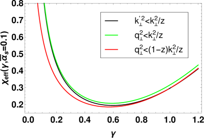
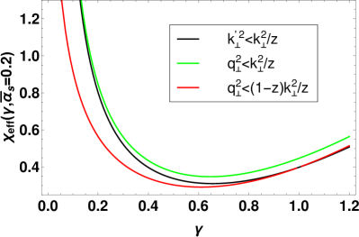
Figure 2: The effective Mellin transformed kernel $\chi_{\rm eff}$ for the three different versions of the kinematical constraint (9),(10),(12) as a function of Mellin variable $\gamma$. Left: $\bar{\alpha}_{s}=0.1$, right plot $\bar{\alpha}_{s}=0.2$.

The first feature of the effective kernels in all cases is that they are strongly modified in the large $\gamma$ region. The results from the constraint (9) and (12) are very close in the $\gamma\simeq 1$ region. Comparing Eq. (66) and (16) we found that they are in fact identical at $\gamma=1$ for any value of $\omega$. One can observe that for $z\rightarrow 1$ both (12) and (9) lead to a strong suppression of the anti-collinear phase-space, i.e. ${k}_{\scaleto{T}{4pt}}^{2}<{k}_{\scaleto{T}{4pt}}^{{}^{\prime}2}$, whereas even for $z\simeq 1$ the constraint (8) leaves some phase space for integration. On the other hand the constraints (10) and (12) are very close in the small $\gamma$ region while the (9) is lower in that range. This can be understood from the fact that in the collinear region, i.e. for ${k}_{\scaleto{T}{4pt}}^{2}>{k}_{\scaleto{T}{4pt}}^{\prime 2}$ the latter constraint is stronger, particularly if $z$ is large.

Next, we have checked numerically the coefficients in front of the poles in $\gamma$ and found agreement between different forms of constraints in the leading $\sim 1/(1-\gamma)^{2k+1}$ and subleading poles $\sim 1/(1-\gamma)^{2k}$ poles when the expressions for the kernels are expanded out to NLL and NNLL .

There is one notable difference between (9) and the other two constraints, in that in the first one the collinear pole in $\gamma$ is absent. This can be understood as for large values of $z>1/2$ constraint (9) implies the restriction of the integration over collinear region as well.

From $\chi_{\rm eff}$ one can find the leading behavior as $x\rightarrow 0$. The intercept which is found from

$$\frac{d\chi_{\rm eff}(\gamma,\bar{\alpha}_{s})}{d\gamma}|_{\gamma=\gamma_{M}}=0\,,\quad\omega_{I\!\!P}=\chi_{\rm eff}(\gamma_{M},\bar{\alpha}_{s})\;,$$ (70)

and is plotted in Fig. 3. All the constraints give similar intercept for values of $\bar{\alpha}_{s}$ up to about $0.2$. The constraint $\eqref{eq:kincon-jk}$ gives somewhat larger values, when $\bar{\alpha}_{s}$ is further increased, while the two constraints $\eqref{eq:kinconorig}$ and $\eqref{eq:kincon-f}$ give comparable values for the intercepts even for very large values of the strong coupling. This is consistent with the shape of the kernel discussed before.

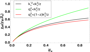
Figure 3: The values of the intercept $\omega_{I\!\!P}=\chi_{\rm eff}(\gamma_{M},\bar{\alpha}_{s})$, Eq. (70), as a function of ${\bar{\alpha}}_{s}$ for different choices of the kinematical constraint.

5 Differential form of the evolution equation with kinematical constraints

The evolution equation in the presence of the kinematical constraint becomes an integral equation, over the longitudinal variable $z$ as is evident from Eq. (60). Equations in this form were solved in the momentum space via different techniques in the past. One technique utilized in the past in Ref. [20] was based on the extension of the method introduced in [54]. This method incorporates the interpolation in two variables $x$ and ${k}_{\scaleto{T}{4pt}}^{2}$ with orthogonal polynomials. By doing this the integral equations can be transformed into the set of linear algebraic equations and solved by simply inverting the large matrix. An alternative method was used in [29] and it was checked that it coincides with the one proposed in [20].

In this paper we shall propose and utilize another method which reduces the integral equation to the differential one. The differentiation of the BFKL equation by $x$ is motivated by the reduction of computational complexity of the integral on the right hand side of the equation. After performing the derivative we find, that no matter what is the form of the kinematical constraint the resulting equation can be written in the differential form and has the same form containing two terms - real emission term with shifted argument $x$ and virtual correction term - under the remaining integral over the emitted momentum ${\bf q}$. The argument of the real emission term is shifted such, that if the kinematical constraint takes the form $\theta\left(k_{C}\left({\bf q},{\bf k}\right)-z\right)$, then the argument of the unintegrated gluon density function in the real emission term changes in following way:

$$x\rightarrow x\;\max\left\{1,\frac{1}{k_{C}\left({\bf q},{\bf k}\right)}\right\}\;.$$ (71)

Such reformulation of the BFKL equation with kinematical constraint was first proposed in [18], and similar ideas were also discussed in [37] in the context of the Balitsky-Kovchegov evolution equation in transverse coordinate space. Below we derive the differential form of the BFKL equation for each case of the kinematical constraint.

Let us begin by differentiating in $x$ the equation with kinematical constraint in the low $z$ approximation, Eq. (10). The equation formally differentiated in $x$ reads

$$\begin{split}\frac{\partial{{\cal F}}(x,{{k}_{\scaleto{T}{4pt}}^{2}})}{\partial x}=\frac{\partial{{\cal F}}_{0}(x,{{k}_{\scaleto{T}{4pt}}^{2}})}{\partial x}&+{\bar{\alpha}_{s}}\frac{\partial}{\partial x}\int\limits_{x}^{1}\frac{dx^{\prime}}{x^{\prime}}\;\int\frac{d^{2}{{\bf q}_{\scaleto{T}{4pt}}}}{\pi{{{q}_{\scaleto{T}{4pt}}}^{2}}}\bigg{\{}{{\cal F}}\left(x^{\prime},|{{\bf k}_{\scaleto{T}{4pt}}}+{{\bf q}_{\scaleto{T}{4pt}}}|^{2}\right)\Theta\left({k}_{\scaleto{T}{4pt}}^{2}-\frac{x}{x^{\prime}}{q}_{\scaleto{T}{4pt}}^{2}\right)\\ &-\,\Theta\left({k}_{\scaleto{T}{4pt}}^{2}-{q}_{\scaleto{T}{4pt}}^{2}\right){{\cal F}}\left(x^{\prime},{{k}_{\scaleto{T}{4pt}}^{2}}\right)\bigg{\}}\;.\end{split}$$ (72)

where we performed the change of variable $z\rightarrow x^{\prime}=x/z$. After performing the derivative we get:

$$\begin{split}\frac{\partial{{\cal F}}(x,{{k}_{\scaleto{T}{4pt}}^{2}})}{\partial x}=&\frac{\partial{{\cal F}}_{0}(x,{{k}_{\scaleto{T}{4pt}}^{2}})}{\partial x}-\frac{{\bar{\alpha}_{s}}}{x}\;\int\frac{d^{2}{{\bf q}_{\scaleto{T}{4pt}}}}{\pi{{{q}_{\scaleto{T}{4pt}}}^{2}}}\bigg{\{}{{\cal F}}\left(x\,\max\left(1,\frac{{q}_{\scaleto{T}{4pt}}^{2}}{{k}_{\scaleto{T}{4pt}}^{2}}\right),|{{\bf k}_{\scaleto{T}{4pt}}}+{{\bf q}_{\scaleto{T}{4pt}}}|^{2}\right)\Theta\left(\frac{{k}_{\scaleto{T}{4pt}}^{2}}{{q}_{\scaleto{T}{4pt}}^{2}}-x\right)\\ -&\,\Theta\left({k}_{\scaleto{T}{4pt}}^{2}-{q}_{\scaleto{T}{4pt}}^{2}\right){{\cal F}}\left(x,{{k}_{\scaleto{T}{4pt}}^{2}}\right)\bigg{\}}\;,\end{split}$$ (73)

where the expression $x\,\max\left(1,\frac{q_{T}^{2}}{k_{T}^{2}}\right)$ emerges from two terms generated by the derivative acting on the integral on the right hand side of the (74). The first one coming from derivative on the boundary of the integral generating term containing ${\cal F}\left(x,|{{\bf k}_{\scaleto{T}{4pt}}}+{{\bf q}_{\scaleto{T}{4pt}}}|^{2}\right)\Theta\left({{k}_{\scaleto{T}{4pt}}^{2}}-{{q}_{\scaleto{T}{4pt}}^{2}}\right)$ and the second one acting on the $\Theta$-function from kinematical constraint generating a term containing ${F}\left(x\frac{{q}_{\scaleto{T}{4pt}}^{2}}{{k}_{\scaleto{T}{4pt}}^{2}},|{{\bf k}_{\scaleto{T}{4pt}}}-{{\bf q}_{\scaleto{T}{4pt}}}|^{2}\right)\Theta\left({{q}_{\scaleto{T}{4pt}}^{2}}-{{k}_{\scaleto{T}{4pt}}^{2}}\right)$ - which combine giving the result in (74).

Rewriting the derivative as a derivative by $\ln{1/x}$ instead of $x$ results in

$$\begin{split}\frac{\partial{{\cal F}}(x,{{k}_{\scaleto{T}{4pt}}^{2}})}{\partial\ln{1/x}}=&\frac{\partial{{\cal F}}_{0}(x,{{k}_{\scaleto{T}{4pt}}^{2}})}{\partial\ln{1/x}}+{\bar{\alpha}_{s}}\;\int\frac{d^{2}{{\bf q}_{\scaleto{T}{4pt}}}}{\pi{{{q}_{\scaleto{T}{4pt}}}^{2}}}\bigg{\{}{{\cal F}}\left(x\,\max\left(1,\frac{{q}_{\scaleto{T}{4pt}}^{2}}{{k}_{\scaleto{T}{4pt}}^{2}}\right),|{{\bf k}_{\scaleto{T}{4pt}}}+{{\bf q}_{\scaleto{T}{4pt}}}|^{2}\right)\Theta\left(\frac{{k}_{\scaleto{T}{4pt}}^{2}}{{q}_{\scaleto{T}{4pt}}^{2}}-x\right)\\ -&\,\Theta\left({k}_{\scaleto{T}{4pt}}^{2}-{q}_{\scaleto{T}{4pt}}^{2}\right){{\cal F}}\left(x,{{k}_{\scaleto{T}{4pt}}^{2}}\right)\bigg{\}}\;.\end{split}$$ (74)

The case of constraint ${k}_{\scaleto{T}{4pt}}^{\prime 2}<{k}_{\scaleto{T}{4pt}}^{2}/z$ can be treated in exactly the same way with the result

$$\begin{split}\frac{\partial{{\cal F}}(x,{{k}_{\scaleto{T}{4pt}}^{2}})}{\partial\ln{1/x}}=&\frac{\partial{{\cal F}}_{0}(x,{{k}_{\scaleto{T}{4pt}}^{2}})}{\partial\ln{1/x}}+{\bar{\alpha}_{s}}\;\int\frac{d^{2}{{\bf q}_{\scaleto{T}{4pt}}}}{\pi{{{q}_{\scaleto{T}{4pt}}}^{2}}}\bigg{\{}{{\cal F}}\left(x\,\max\left(1,\frac{{k}_{\scaleto{T}{4pt}}^{{}^{\prime}2}}{{k}_{\scaleto{T}{4pt}}^{2}}\right),|{{\bf k}_{\scaleto{T}{4pt}}}+{{\bf q}_{\scaleto{T}{4pt}}}|^{2}\right)\Theta\left(\frac{{k}_{\scaleto{T}{4pt}}^{2}}{{k}_{\scaleto{T}{4pt}}^{{}^{\prime}2}}-x\right)\\ -&\,\Theta\left({k}_{\scaleto{T}{4pt}}^{2}-{q}_{\scaleto{T}{4pt}}^{2}\right){{\cal F}}\left(x,{{k}_{\scaleto{T}{4pt}}^{2}}\right)\bigg{\}}\;.\end{split}$$ (75)

Thus we see very intersting result in that the entire effect of the kinematical constraint is to shift the longitudinal variable in the argument of the unintegrated gluon density in the real term by a factor which includes a combination of ratio of transverse momenta.

The case with the kinematical constraint ${q}_{\scaleto{T}{4pt}}^{2}<\frac{1-z}{z}{k}_{\scaleto{T}{4pt}}^{2}$ is a bit different, since in this case the term originating from the derivative acting on the integral boundary is equal to $0$. This is because of the $\Theta$-function being evaluated at $-\infty$. In other words, this constraint means that $x^{\prime}>x\frac{k_{T}^{2}+q_{T}^{2}}{k_{T}^{2}}$ which is always stronger than $x^{\prime}>x$ and therefore the boundary term will not contribute here. This results in the following differential equation

$$\begin{split}\frac{\partial{{\cal F}}(x,{{k}_{\scaleto{T}{4pt}}^{2}})}{\partial\ln{1/x}}=\frac{\partial{{\cal F}}_{0}(x,{{k}_{\scaleto{T}{4pt}}^{2}})}{\partial\ln{1/x}}&+{\bar{\alpha}_{s}}\int\frac{d^{2}{{\bf q}_{\scaleto{T}{4pt}}}}{\pi{{{q}_{\scaleto{T}{4pt}}}^{2}}}\bigg{\{}{{\cal F}}\left(x\,\frac{{k}_{\scaleto{T}{4pt}}^{2}+{q}_{\scaleto{T}{4pt}}^{2}}{{k}_{\scaleto{T}{4pt}}^{2}},|{{\bf k}_{\scaleto{T}{4pt}}}+{{\bf q}_{\scaleto{T}{4pt}}}|^{2}\right)\Theta\left(\frac{{k}_{\scaleto{T}{4pt}}^{2}}{{q}_{\scaleto{T}{4pt}}^{2}+{k}_{\scaleto{T}{4pt}}^{2}}-x\right)\\ &-\,\Theta\left({k}_{\scaleto{T}{4pt}}^{2}-{q}_{\scaleto{T}{4pt}}^{2}\right){{\cal F}}\left(x,{{k}_{\scaleto{T}{4pt}}^{2}}\right)\bigg{\}}\;.\end{split}$$ (76)

6 Numerical method and results

6.1 Numerical results

In this section we shall present the numerical results for the solution of the BFKL equation with different forms of the kinematical constraint. The details for the numerical method are described in the Appendix. The equations are solved using the boundary condition

$${\mathcal{F}}\left(x,k_{T}\right)=\exp\left[p_{0}\log{(k_{T}/\mu)}^{2}+p_{1}\log^{2}{(k_{T}/\mu)}^{2}\right]\left(1-x\right)^{p_{2}}\;,$$ (77)

with $p_{0}=p_{1}=-0.1$ and $p_{2}=2$ and $\mu=1\,{\rm GeV}$. Since we are not doing any phenomenology here this boundary condition has not being fitted to any data and is for illustrative purposes only. The particular choice of $k_{T}$ dependence is motivated by analitical solution of the LO BFKL equation and guarantes fast convergence of the solution. The term $(1-x)^{p_{2}}$ guaantees that the gluon is suppressed for large values of $x$ so that the integral over the kernel can be extended to large $x$ values. We introduce the lower cutoff onto the transverse momenta $Q_{0}=0.1\;{\rm GeV}$. The results were obtained for the fixed value of the coupling constant $\bar{\alpha}_{s}=0.2$.

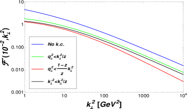
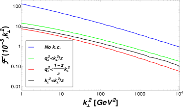
Figure 4: Solutions of the BFKL equations with different forms of the kinematical constraint as functions of $k_{T}$ for constant ${\bar{\alpha}}_{S}=0.2$. Left plot: $x=10^{-2}$, right plot: $x=10^{-5}$.

The results for the solution as a function of the ${k}_{\scaleto{T}{4pt}}^{2}$ for fixed values of $x$ and different forms of the kinematical constraint are shown in plots in Figs. 4 together with the solution to the LL BFKL. The results reflect the trend of the semi-analytical results from the section 4. In plots of ${{k}_{\scaleto{T}{4pt}}}^{2}$ dependence for $x=10^{-2}$ it is clear that the solution with the full kinematical constraint and the solution of the equation with the kinematical constraint in the ${k}_{\scaleto{T}{4pt}}^{\prime 2}<k_{T}^{2}/z$ approximation get close to each other for low ${k_{T}}^{2}$. On the other hand, for large values of ${k}_{\scaleto{T}{4pt}}^{2}$ it is the two constraints (10) and (9) which come close to each other and (9) has a different behavior. This is related to the different behavior in the collinear limit, i.e. the fact that constraint (9) introduces modification in the collinear limit as well as discussed previously. In any case the solution with the constraint (10) always leads to the results which is largest, consistent with the analysis from the Mellin space. Similar conclusions can be reached from the analysis of the plots with the $x$ dependence for small ${k_{T}}^{2}$ shown in Figs.(5). The small $z$ approximation of the kinematical constraint results in the solution being closer to the solution of the equation with the ${q_{T}}^{2}\simeq{k^{\prime}_{T}}^{2}$ approximation of the kinematical constraint for large ${k_{T}}^{2}$. From Fig.(5) we see the onset of the power behaviour in $x$, and in all versions of the kinematical constraint the intercept is strongly reduced with respect to the LL approximation. The differences between the solutions with different versions of the kinematical constraint are much smaller than between resummed and LL result. Nevertheless, the differences between different versions of the kinematical constraint are non-negligible and can reach up to a factor 2-3 depending on the range of $x$ and ${k}_{\scaleto{T}{4pt}}$.

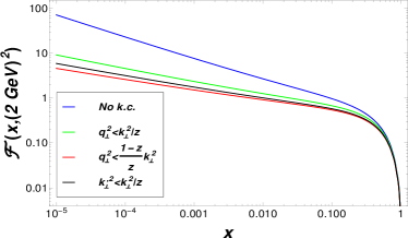
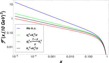
Figure 5: Solutions to the BFKL equation with three different forms of the constraint as a function of $x$ for constant ${\bar{\alpha}}_{S}=0.2$. Left plot: ${k}_{\scaleto{T}{4pt}}=2\,{\rm GeV}$, right plot ${k}_{\scaleto{T}{4pt}}=10\,{\rm GeV}$.

Conclusions

In the paper we have performed a detailed analysis of the three versions of kinematical constraints imposed onto the momentum space BFKL equation. We used the fixed coupling BFKL equation as a basic equation on which kernel’s the constrains are imposed. This choice allowed us to investigate semi-analytically the properties of the kinematical constrains in the Mellin space and to compare to known results in sYM version of the BFKL equations where the results are known up to NNLL order. In particular, we observed that the leading poles in Mellin space generated by the kinematical constraint obey maximal transcendentality principle. In addition we proved that the subleading poles vanish at NLL and NNLL order both for BFKL and its sYM version, and that such feature can be expected to hold to all orders. Furthermore we observed that the $\chi_{eff}$ function obtained with the most general version of the constraint i.e. (9) for large values of $\gamma$ agrees well with the more commonly used version of the constraint i.e (12). However, at small values of $\gamma$ the $\chi_{eff}$ function with (12) agrees with (10) and both of them differ from the case when constraint (9) is imposed. In particular, it is important to note that the last one changes the collinear structure of the kernel i.e. it limits $z$ to $z<1/2$. While on formal grounds this effect might be neglected in the small $z$ limit it has nonnegligible impact on the resulting gluon density. We demonstrate that by numerical solutions of the momentum space BFKL equation for unintegrated gluon density for all versions of the constraint as well as for the unmodified BFKL equation. The understanding of action of the kinematical constraint across the whole region of $z$ will be particularly important for ongoing efforts to unify the BFKL and DGLAP evolution schemes [55, 56, 57] where effects of kinematical constrains may play a crucial role. Furthermore, the inclusion of the kinematical constraint is known to be relevant for BFKL phenomenology [20, 58, 59, 60, 61, 62, 63]. However, so far only the simplest version of it was used in the context of BFKL. It will be interesting to see how different versions of the constraint perform while a fit to $F_{2}$ data is done or what are the differences when the description of processes probing gluon density at very low $x$ like high energy neutrinos or very forward dijet data is attempted.

Appendix

Algebraic form of the equation suitable for numerical solution

In order to solve the equation we shall use the method of expansion in the set of Chebyshev polynomials in the ${k}_{\scaleto{T}{4pt}}$ variable. Using this interpolation we can expand a function on the interval $[-1,1]$ in the following way

$$\begin{split}f\left(\zeta\right)=\sum\limits_{j=0}^{N-1}f\left(\zeta_{j}\right)c_{j}\left(\zeta,N\right)=\sum\limits_{j=0}^{N-1}f_{j}\,c_{j}\left(\zeta,N\right)\;,\end{split}$$ (78)

where

$$c_{j}\left(\zeta,N\right)=\frac{2}{N}\sum\limits_{i=0}^{N-1}T_{i}\left(\zeta_{j}\right)T_{i}\left(\zeta\right)o_{i}\;,$$ (79)

with $T_{i}\left(\zeta\right)$ a Chebyshev polynomial of the $i$-th order, $\zeta_{j}$ are nodes of the Chebyshev polynomial of the $N$-th order,i.e. $\zeta_{j}=\cos((j+\frac{1}{2})\frac{\pi}{N})$ and finally $o_{i}=1/2$ for $i=0$ and $o_{i}=1$ for $i>0$. In the following, we use the unintegrated gluon distribution functions which are averaged over the angle, i.e. the dependence is only on ${k}_{\scaleto{T}{4pt}}^{2}$. Let us first rewrite the equation (76) using the expansion of the function ${F}\left(x,{{k}_{\scaleto{T}{4pt}}^{2}}\right)$ in ${k}_{\scaleto{T}{4pt}}$ on a grid of Chebyshev nodes and in $x$ with trapezoidal interpolation

$$\begin{split}\frac{\partial{{\cal F}}(x,{{k}_{\scaleto{T}{4pt}}}_{i}^{2})}{\partial\ln{x}}\bigg{|}_{x=x_{j}}&=\frac{\partial{{\cal F}}_{0}(x,{{k}_{\scaleto{T}{4pt}}}_{i}^{2})}{\partial\ln{x}}\bigg{|}_{x=x_{j}}\\ -\sum\limits_{m=0}^{N_{k}-1}\sum\limits_{n=0}^{N_{x}-1}{\bar{\alpha}_{s}}&\int\frac{d^{2}{{\bf q}_{\scaleto{T}{4pt}}}}{\pi{{{q}_{\scaleto{T}{4pt}}}^{2}}}\left\{{{\cal F}}\left(x_{n},{{k}_{\scaleto{T}{4pt}}^{2}}_{m}\right)t\left(x_{j}\,\frac{{{k}_{\scaleto{T}{4pt}}^{2}}_{i}+{q}_{\scaleto{T}{4pt}}^{2}}{{{k}_{\scaleto{T}{4pt}}^{2}}_{i}},n\right)c_{m}\left(\zeta\left(|{{\bf k}_{\scaleto{T}{4pt}}}_{i}-{{\bf q}_{\scaleto{T}{4pt}}}|\right),N_{k}\right)\right.\\ &\qquad-\,\left.\Theta\left({{k}_{\scaleto{T}{4pt}}}^{2}_{i}-{q}_{\scaleto{T}{4pt}}^{2}\right){{\cal F}}\left(x_{n},{{k}_{\scaleto{T}{4pt}}^{2}}_{m}\right)t\left(x_{j},n\right)c_{m}\left(\zeta\left({{k}_{\scaleto{T}{4pt}}}_{i}\right),N_{k}\right)\right\}\;,\end{split}$$ (80)

where ${{k}_{\scaleto{T}{4pt}}}_{m}$ are values projected from Chebyshev nodes on the ${k}_{\scaleto{T}{4pt}}$-space, whereas $\zeta\left({{k}_{\scaleto{T}{4pt}}}_{i}\right)$ is the projection of the momentum ${k}_{\scaleto{T}{4pt}}$ on the interval of $[-1,1]$ interval, suitable for Chebyshev interpolation. The integers $N_{x}$ and $N_{k}$ are the numbers of grid points in $x$ and ${k}_{\scaleto{T}{4pt}}$ ranges respectively. Finally we define the function $t\left(x,n\right)$ which is a combination of triangular functions providing the trapezoidal interpolation in $\ln{x}$:

$$\begin{split}t\left(x,n\right)=&\ln{\left(x/x_{n+1}\right)}/\ln{\left(x_{n}/x_{n+1}\right)}\Theta\left(x-x_{n+1}\right)\Theta\left(x_{n}-x\right)\\ +&\ln{\left(x_{n-1}/x\right)}/\ln{\left(x_{n-1}/x_{n}\right)}\Theta\left(x_{n-1}-x\right)\Theta\left(x-x_{n}\right)\;.\end{split}$$ (81)

Further rewriting (80) into the matrix form results into this form of the equation

We define a matrix

$$\begin{split}{\bar{K}}_{ij;mn}=&{\bar{\alpha}}_{s}\int\frac{d^{2}{\bf q}}{\pi{{\bf q}^{2}}}\left\{t\left(x\frac{{k^{2}_{T}}_{i}+q^{2}_{T}}{{k^{2}_{T}}_{i}},n\right)c_{m}\left(\zeta\left(|{\bf k}_{i}-{\bf q}|\right),N_{k}\right)\right.\\ &\qquad-\,\left.\theta\left({k_{T}}^{2}_{i}-q_{T}^{2}\right)t\left(x_{j},n\right)c_{m}\left(\zeta\left({k_{T}}_{i}\right),N_{k}\right)\right\}\;\end{split}$$ (82)

and finally write:

$$\begin{split}\frac{\partial{\cal F}(x,{k_{T}}_{i}^{2})}{\partial\ln{x}}\bigg{|}_{x=x_{j}}&=\frac{\partial{\cal F}_{0}(x,{k_{T}}_{i}^{2})}{\partial\ln{x}}\bigg{|}_{x=x_{j}}-\sum\limits_{m=0}^{N_{k}-1}\sum\limits_{n=0}^{N_{x}-1}\,{\bar{K}}_{ij;mn}\,\mathcal{F}_{mn}\;.\end{split}$$ (83)

To solve the equation we can use the discretized form of the differential of the function ${\cal F}(x,{k_{T}}_{i}^{2})$ in $\ln{x}$:

$$\begin{split}{\cal F}\left(x\,(1+d\ln{x}),{k_{T}}_{i}^{2}\right)=\,&{\cal F}\left(x,{k_{T}}_{i}^{2}\right)+\frac{\partial{\cal F}\left(x,{k_{T}}_{i}^{2}\right)}{\partial\ln{x}}d\ln{x}\;\\ \downarrow&\\ {\cal F}\left(x_{j+1},{k_{T}}_{i}^{2}\right)=\,&{\cal F}\left(x_{j},{k_{T}}_{i}^{2}\right)+\frac{\partial{\cal F}\left(x,{k_{T}}_{i}^{2}\right)}{\partial\ln{x}}\bigg{|}_{x=x_{j}}\ln{\left(\frac{x_{j+1}}{x_{j}}\right)}\;.\end{split}$$ (84)

The equation above (84) together with (83) with the boundary condition ${\cal F}\left(x_{0},{k_{T}}_{i}^{2}\right)={\cal F}_{0}\left(x_{0},{k_{T}}_{i}^{2}\right)$ can be used to solve the equation (76) numerically using the iteration method. The algorithm can be summarized in the following diagram:

$$\begin{split}&\qquad{\cal F}\left(x_{j},{k_{T}}_{i}^{2}\right)\\ &\eqref{eq:numderivative}\downarrow\qquad\qquad\uparrow\eqref{eq:differential}\\ &\qquad\frac{\partial{\cal F}(x,{k_{T}}_{i}^{2})}{\partial\ln{x}}\bigg{|}_{x=x_{j}}\end{split}$$ (85)

Distance between the values of ${\cal F}\left(x_{j},{k_{T}}_{i}^{2}\right)$ in two subsequent cycles is evaluated after each cycle and the algorithm is terminated when the distance becomes sufficiently small.

We parametrize the grid points in following ways:

$$\begin{split}x_{j}=\,&x_{max}\exp{\left[-\frac{j}{N_{x}-1}\log\frac{x_{max}}{x_{min}}\right]}\;,\\ {k_{T}}_{i}=\,&Q_{0}\,\exp\left[\frac{\zeta_{i}+1}{2}\log\frac{w}{Q_{0}}\right]\;,\end{split}$$ (86)

with $x_{max}$ and $x_{min}$ being the upper and lower limit of the $x$-axis of the grid, $w$ and $Q_{0}$ being the upper and lower limit of the $k_{T}$-axis of the grid and $\zeta_{i}=\cos\left(\frac{\pi(i+1/2)}{N_{k}}\right)$ being the Chebyshev node.

References

- [1] I. Abt et al., “Measurement of the proton structure function F2 (x, Q**2) in the low x region at HERA,” Nucl. Phys., vol. B407, pp. 515–538, 1993.
- [2] M. Derrick et al., “Measurement of the proton structure function F2 in e p scattering at HERA,” Phys. Lett., vol. B316, pp. 412–426, 1993.
- [3] J. C. Collins, D. E. Soper, and G. F. Sterman, “Factorization of Hard Processes in QCD,” Adv. Ser. Direct. High Energy Phys., vol. 5, pp. 1–91, 1989.
- [4] V. N. Gribov and L. N. Lipatov, “Deep inelastic e p scattering in perturbation theory,” Sov. J. Nucl. Phys., vol. 15, pp. 438–450, 1972. [Yad. Fiz.15,781(1972)].
- [5] G. Altarelli and G. Parisi, “Asymptotic Freedom in Parton Language,” Nucl. Phys., vol. B126, pp. 298–318, 1977.
- [6] Y. L. Dokshitzer, “Calculation of the Structure Functions for Deep Inelastic Scattering and e+ e- Annihilation by Perturbation Theory in Quantum Chromodynamics.,” Sov. Phys. JETP, vol. 46, pp. 641–653, 1977. [Zh. Eksp. Teor. Fiz.73,1216(1977)].
- [7] R. D. Ball, V. Bertone, M. Bonvini, S. Marzani, J. Rojo, and L. Rottoli, “Parton distributions with small-x resummation: evidence for BFKL dynamics in HERA data,” Eur. Phys. J., vol. C78, no. 4, p. 321, 2018.
- [8] L. N. Lipatov, “The Bare Pomeron in Quantum Chromodynamics,” Sov. Phys. JETP, vol. 63, pp. 904–912, 1986. [Zh. Eksp. Teor. Fiz.90,1536(1986)].
- [9] E. A. Kuraev, L. N. Lipatov, and V. S. Fadin, “The Pomeranchuk Singularity in Nonabelian Gauge Theories,” Sov. Phys. JETP, vol. 45, pp. 199–204, 1977. [Zh. Eksp. Teor. Fiz.72,377(1977)].
- [10] I. I. Balitsky and L. N. Lipatov, “The Pomeranchuk Singularity in Quantum Chromodynamics,” Sov. J. Nucl. Phys., vol. 28, pp. 822–829, 1978. [Yad. Fiz.28,1597(1978)].
- [11] L. N. Lipatov, “Small x physics in perturbative QCD,” Phys. Rept., vol. 286, pp. 131–198, 1997.
- [12] V. S. Fadin and L. N. Lipatov, “BFKL pomeron in the next-to-leading approximation,” Phys. Lett., vol. B429, pp. 127–134, 1998.
- [13] M. Ciafaloni and G. Camici, “Energy scale(s) and next-to-leading BFKL equation,” Phys. Lett., vol. B430, pp. 349–354, 1998.
- [14] N. Gromov, F. Levkovich-Maslyuk, and G. Sizov, “Pomeron Eigenvalue at Three Loops in 4 Supersymmetric Yang-Mills Theory,” Phys. Rev. Lett., vol. 115, no. 25, p. 251601, 2015.
- [15] V. N. Velizhanin, “BFKL pomeron in the next-to-next-to-leading approximation in the planar N=4 SYM theory,” 2015.
- [16] S. Caron-Huot and M. Herranen, “High-energy evolution to three loops,” Journal of High Energy Physics, vol. 2018, no. 2, p. 58, 2018.
- [17] M. Ciafaloni, “Coherence Effects in Initial Jets at Small q**2 / s,” Nucl. Phys., vol. B296, pp. 49–74, 1988.
- [18] B. Andersson, G. Gustafson, and J. Samuelsson, “The Linked dipole chain model for DIS,” Nucl. Phys., vol. B467, pp. 443–478, 1996.
- [19] J. Kwiecinski, A. D. Martin, and P. J. Sutton, “Constraints on gluon evolution at small x,” Z. Phys., vol. C71, pp. 585–594, 1996.
- [20] J. Kwiecinski, A. D. Martin, and A. M. Stasto, “A Unified BFKL and GLAP description of F2 data,” Phys. Rev., vol. D56, pp. 3991–4006, 1997.
- [21] G. P. Salam, “A Resummation of large subleading corrections at small x,” JHEP, vol. 07, p. 019, 1998.
- [22] G. Altarelli, R. D. Ball, and S. Forte, “Resummation of singlet parton evolution at small x,” Nucl. Phys., vol. B575, pp. 313–329, 2000.
- [23] G. Altarelli, R. D. Ball, and S. Forte, “Small x resummation and HERA structure function data,” Nucl. Phys., vol. B599, pp. 383–423, 2001.
- [24] G. Altarelli, R. D. Ball, and S. Forte, “Factorization and resummation of small x scaling violations with running coupling,” Nucl. Phys., vol. B621, pp. 359–387, 2002.
- [25] G. Altarelli, R. D. Ball, and S. Forte, “An Anomalous dimension for small x evolution,” Nucl. Phys., vol. B674, pp. 459–483, 2003.
- [26] G. Altarelli, R. D. Ball, and S. Forte, “Small x Resummation with Quarks: Deep-Inelastic Scattering,” Nucl. Phys., vol. B799, pp. 199–240, 2008.
- [27] M. Ciafaloni, D. Colferai, and G. P. Salam, “A collinear model for small x physics,” JHEP, vol. 10, p. 017, 1999.
- [28] M. Ciafaloni, D. Colferai, and G. P. Salam, “Renormalization group improved small x equation,” Phys. Rev., vol. D60, p. 114036, 1999.
- [29] M. Ciafaloni, D. Colferai, G. P. Salam, and A. M. Stasto, “Renormalization group improved small x Green’s function,” Phys. Rev., vol. D68, p. 114003, 2003.
- [30] M. Ciafaloni, D. Colferai, G. P. Salam, and A. M. Stasto, “The Gluon splitting function at moderately small x,” Phys. Lett., vol. B587, pp. 87–94, 2004.
- [31] M. Ciafaloni, D. Colferai, G. P. Salam, and A. M. Stasto, “A Matrix formulation for small-x singlet evolution,” JHEP, vol. 08, p. 046, 2007.
- [32] A. Sabio Vera, “An ’All-poles’ approximation to collinear resummations in the Regge limit of perturbative QCD,” Nucl. Phys., vol. B722, pp. 65–80, 2005.
- [33] M. Bonvini, S. Marzani, and T. Peraro, “Small- resummation from HELL,” Eur. Phys. J., vol. C76, no. 11, p. 597, 2016.
- [34] R. S. Thorne, “The Running coupling BFKL anomalous dimensions and splitting functions,” Phys. Rev., vol. D64, p. 074005, 2001.
- [35] C. D. White and R. S. Thorne, “A Global Fit to Scattering Data with NLL BFKL Resummations,” Phys. Rev., vol. D75, p. 034005, 2007.
- [36] L. Motyka and A. M. Stasto, “Exact kinematics in the small x evolution of the color dipole and gluon cascade,” Phys. Rev., vol. D79, p. 085016, 2009.
- [37] G. Beuf, “Improving the kinematics for low- QCD evolution equations in coordinate space,” Phys. Rev., vol. D89, no. 7, p. 074039, 2014.
- [38] E. Iancu, J. D. Madrigal, A. H. Mueller, G. Soyez, and D. N. Triantafyllopoulos, “Resumming double logarithms in the QCD evolution of color dipoles,” Phys. Lett., vol. B744, pp. 293–302, 2015.
- [39] Y. Hatta and E. Iancu, “Collinearly improved JIMWLK evolution in Langevin form,” JHEP, vol. 08, p. 083, 2016.
- [40] F. Hautmann, H. Jung, and S. T. Monfared, “The CCFM uPDF evolution uPDFevolv Version 1.0.00,” Eur. Phys. J., vol. C74, p. 3082, 2014.
- [41] S. Catani, F. Fiorani, and G. Marchesini, “Small x Behavior of Initial State Radiation in Perturbative QCD,” Nucl. Phys., vol. B336, pp. 18–85, 1990.
- [42] S. Catani, F. Fiorani, and G. Marchesini, “QCD Coherence in Initial State Radiation,” Phys. Lett., vol. B234, pp. 339–345, 1990.
- [43] G. Marchesini, “QCD coherence in the structure function and associated distributions at small x,” Nucl. Phys., vol. B445, pp. 49–80, 1995.
- [44] H. Jung et al., “The CCFM Monte Carlo generator CASCADE version 2.2.03,” Eur. Phys. J., vol. C70, pp. 1237–1249, 2010.
- [45] Y. L. Dokshitzer, V. A. Khoze, S. I. Troian, and A. H. Mueller, “QCD Coherence in High-Energy Reactions,” Rev. Mod. Phys., vol. 60, p. 373, 1988.
- [46] M. Ciafaloni, D. Colferai, D. Colferai, G. P. Salam, and A. M. Stasto, “Extending QCD perturbation theory to higher energies,” Phys. Lett., vol. B576, pp. 143–151, 2003.
- [47] K. J. Golec-Biernat, L. Motyka, and A. M. Stasto, “Diffusion into infrared and unitarization of the BFKL pomeron,” Phys. Rev., vol. D65, p. 074037, 2002.
- [48] K. Kutak and J. Kwiecinski, “Screening effects in the ultrahigh-energy neutrino interactions,” Eur. Phys. J., vol. C29, p. 521, 2003.
- [49] L. H. Orr and W. J. Stirling, “Dijet production at hadron hadron colliders in the BFKL approach,” Phys. Rev., vol. D56, pp. 5875–5884, 1997.
- [50] J. R. Andersen and W. J. Stirling, “Energy consumption and jet multiplicity from the leading log BFKL evolution,” JHEP, vol. 02, p. 018, 2003.
- [51] E. Avsar, G. Gustafson, and L. Lonnblad, “Energy conservation and saturation in small-x evolution,” JHEP, vol. 07, p. 062, 2005.
- [52] A. V. Kotikov and L. N. Lipatov, “DGLAP and BFKL evolution equations in the N=4 supersymmetric gauge theory,” Nuclear Physics B, vol. 661, pp. 19–61, June 2003. arXiv: hep-ph/0208220.
- [53] S. Marzani, R. D. Ball, P. Falgari, and S. Forte, “BFKL at next-to-next-to-leading order,” Nucl. Phys., vol. B783, pp. 143–175, 2007.
- [54] J. Kwiecinski and D. Strozik-Kotlorz, “Possible Parametrization of Parton Distributions Incorporating Singular Small X Behavior Implied by QCD and Its Phenomenological Implications for HERA,” Z. Phys., vol. C48, pp. 315–326, 1990.
- [55] O. Gituliar, M. Hentschinski, and K. Kutak, “Transverse-momentum-dependent quark splitting functions in factorization: real contributions,” JHEP, vol. 01, p. 181, 2016.
- [56] M. Hentschinski, A. Kusina, and K. Kutak, “Transverse momentum dependent splitting functions at work: quark-to-gluon splitting,” Phys. Rev., vol. D94, no. 11, p. 114013, 2016.
- [57] M. Hentschinski, A. Kusina, K. Kutak, and M. Serino, “TMD splitting functions in factorization: the real contribution to the gluon-to-gluon splitting,” Eur. Phys. J., vol. C78, no. 3, p. 174, 2018.
- [58] M. Hentschinski, A. Sabio Vera, and C. Salas, “ and at small using a collinearly improved BFKL resummation,” Phys. Rev., vol. D87, no. 7, p. 076005, 2013.
- [59] A. van Hameren, P. Kotko, K. Kutak, and S. Sapeta, “Small- dynamics in forward-central dijet decorrelations at the LHC,” Phys. Lett., vol. B737, pp. 335–340, 2014.
- [60] E. Iancu, J. D. Madrigal, A. H. Mueller, G. Soyez, and D. N. Triantafyllopoulos, “Collinearly-improved BK evolution meets the HERA data,” Phys. Lett., vol. B750, pp. 643–652, 2015.
- [61] A. van Hameren, P. Kotko, and K. Kutak, “Resummation effects in the forward production of Z0+jet at the LHC,” Phys. Rev., vol. D92, no. 5, p. 054007, 2015.
- [62] A. van Hameren, P. Kotko, K. Kutak, and S. Sapeta, “Broadening and saturation effects in dijet azimuthal correlations in p-p and p-Pb collisions at 5.02 TeV,” 2019.
- [63] P. Phukan, M. Lalune, and J. K. Sarma, “Small phenomenology on gluon evolution through BFKL equation in light of a constraint in multi-Regge kinematics,” 2019.