Sharp Bounds on the Runtime of the (1+1) EA via Drift Analysis and Analytic Combinatorial Tools

Abstract

The expected running time of the classical (1+1) EA on the OneMax benchmark function has recently been determined by Hwang et al. (2018) up to additive errors of $O((\log n)/n)$. The same approach proposed there also leads to a full asymptotic expansion with errors of the form $O(n^{-K}\log n)$ for any $K>0$. This precise result is obtained by matched asymptotics with rigorous error analysis (or by solving asymptotically the underlying recurrences via inductive approximation arguments), ideas radically different from well-established techniques for the running time analysis of evolutionary computation such as drift analysis. This paper revisits drift analysis for the (1+1) EA on OneMax and obtains that the expected running time $\mathord{E}\hskip 1.29167pt\mathord{\left(T\right)}$, starting from $\lceil n/2\rceil$ one-bits, is determined by the sum of inverse drifts up to logarithmic error terms, more precisely

$$\sum_{k=1}^{\lfloor n/2\rfloor}\frac{1}{\Delta(k)}-c_{1}\log n\leq\mathord{E}\hskip 1.29167pt\mathord{\left(T\right)}\leq\sum_{k=1}^{\lfloor n/2\rfloor}\frac{1}{\Delta(k)}-c_{2}\log n$$

where $\Delta(k)$ is the drift (expected increase of the number of one-bits from the state of $n-k$ ones) and $c_{1},c_{2}\,>0$ are explicitly computed constants. This improves the previous asymptotic error known for the sum of inverse drifts from $\tilde{O}(n^{2/3})$ to a logarithmic error and gives for the first time a non-asymptotic error bound. Using standard asymptotic techniques, the difference between $\mathord{E}\hskip 1.29167pt\mathord{\left(T\right)}$ and the sum of inverse drifts is found to be $(e/2)\log n+O(1)$.

1 Introduction

The runtime analysis of randomized search heuristics on simple, well-structured benchmark problems has triggered the development of analytical tools for understanding the complexity and considerably contributed to their theoretical foundations. This paper is concerned with the objective function $\textsc{OneMax}(x_{1},\dots,x_{n})=x_{1}+\dots+x_{n}$, the arguably most fundamental theoretical benchmark problem in discrete search spaces and the (1+1) EA, probably the most fundamental search heuristic in the theoretical runtime analysis (see Algorithm 1).

Already the earliest analysis of the (1+1) EA [26] showed that the (1+1) EA optimizes OneMax in an expected time of $O(n\log n)$, where time corresponds to the number of iterations. The early interest and attempts in obtaining more precise description of the runtime complexity were summarized in Garnier et al.’s fine paper [10] with very strong approximation results claimed. On the other hand, it follows from the analyses in [9] that the expected time is bounded from above by $enH_{n}\leq en(\log n+1)$, where $H_{n}=\sum_{j=1}^{n}1/j$ denotes the $n$-th harmonic number and $\log n$ the natural logarithm. Lower bounds of the kind $\Omega(n\log n)$ that hold for the much larger class of functions with a unique optimum [9] showed that the results were at least asymptotically tight.

From the beginning of this decade, finer analyses of the expected runtimes have gained increasing attention. Precise expressions for the runtime, dependent not only on the search space dimension $n$ but also on parameters such as the mutation rate, are vital to optimize parameter settings [29] and to compare different algorithms whose runtime only differs in lower-order terms [4].

With respect to OneMax, the first lower bound that explicitly states the leading coefficient $e$ in an expression of the type ${(1-o(1))en\log n}$ was independently derived by Doerr, Fouz and Witt [5] and Sudholt [28] (in the finer form $en\log n-2n\log\log n$) using the techniques of drift analysis and fitness levels, respectively. The lower-order term was sharpened to a linear term $\Omega(n)$ in [6], and an explicit bound for the coefficient of this linear term, was given by Lehre and Witt [23], who proved the lower bound $en\log n-7.81791n-O(\log n)$. The main tool to derive these results relies on increasingly refined drift theorems, most notably on variable drift analysis. At roughly the same time, Hwang et al. [14] presented a drastically refined analysis, which determines the expected runtime of the (1+1) EA on OneMax up to terms of order $O((\log n)/n)$: the exact expression given is

$$en\log n-C_{1}n+(e/2)\log n+C_{2}+O((\log n)/n),$$ (1)

where $C_{1}=1.89254\dots$ and $C_{2}=0.59789875\dots$ are explicitly computable constants; see also [15] for the journal version and http://140.109.74.92/hk/?p=840 for the web version with a full asymptotic expansion. To obtain these precise results, techniques fundamentally different from drift analysis and other established methods for the runtime analysis were used, namely matched asymptotics with rigorous error analysis. In addition to the expected runtime, the asymptotic variance as well as the limiting distribution are also worked out there by similar approaches.

While the expression for the asymptotic expected runtime in (1) represents the best of its kind, it also raises important open questions. First, from a more didactical and methodological point of view, one may look for a more elementary derivation of the formula (1), at least with respect to the linear term $-C_{1}n$. Note that one can analyze the related search heuristic RLS, which flips exactly one bit per iteration, on OneMax exactly and without any asymptotic terms (see [3]), at least if it is initialized deterministically with $\lceil n/2\rceil$ one-bits. The expression of the expected runtime equals $nH_{\lfloor n/2\rfloor}$ then and is accompanied by an intuitive proof appealing to the coupon collector theorem. For a uniform initialization, the analysis become more involved but still an extremely precise result (coming with an asymptotic term, though) exists: $nH_{\lfloor n/2\rfloor}-1/2+o(1)$. This proof takes only a few pages and uses well-known intuitive concepts such as the binomial distribution. The $o(1)$-term comes without an explicit error bound, though, and it is not discussed how to refine it.

Second, it would be helpful to confirm that the constant in the $O((\log n)/n)$-term is small so that one may call it negligible even for small problem sizes. This question may be approached along two different directions: one via an explicit error bound for all $n$, and the other by combining exact numerical calculations and asymptotic expansions. The former will be realized by the drift analysis presented in Sections 3–4 of this paper; we briefly describe here the latter, which depends on the sample size $n$. If $n$ is large enough, say $n\geq 50$, then we can use a longer expansion of the form

$$en\log n-C_{1}n+\sum_{0\leq k\leq K}\frac{d_{k}\log n+e_{k}}{n^{k}}$$

where $K$ is chosen large enough depending on the required tolerance error. In particular, by refining the analysis in [15], one has $d_{0}=\frac{1}{2}$, $d_{1}=\frac{9}{8}$ and $d_{2}=\frac{31}{16}$ (expressions for $e_{k}$ being more complex). On the other hand, if $n$ is small, one can always compute the exact quantity by the underlying recurrence relations without introducing any error. Such an exact calculation can be made efficient even in portable computing devices such as laptops and for $n$ in the hundreds; it is equally helpful in measuring the error introduced when using $K$ terms of the asymptotic expansion.

While different approaches have their own strengths and weaknesses, it is possible to combine them in many cases in discrete probabilities and algorithmics, and obtain results that are often stronger than a single approach can achieve. The fine approximation we work out in this paper represents another testimony to this statement.

Our contribution.

In this paper, we revisit the method of drift analysis and obtain that the expected runtime $\mathord{E}\hskip 1.29167pt\mathord{\left(T\right)}$ of the (1+1) EA on OneMax, started from $\lceil n/2\rceil$ ones, is approximated by the sum of inverse drifts up to logarithmic error terms, more precisely

$$\sum_{k=1}^{\lfloor n/2\rfloor}\frac{1}{\Delta(k)}-c_{1}\log n\leq\mathord{E}\hskip 1.29167pt\mathord{\left(T\right)}\leq\sum_{k=1}^{\lfloor n/2\rfloor}\frac{1}{\Delta(k)}-c_{2}\log n,$$

where $\Delta(k)$ is the drift (expected increase of the number of one-bits from the state of $n-k$ ones) and $c_{1},c_{2}\,>0$ are explicitly computed constants. This gives not only an intuitive approximation of the expected runtime via inverse drifts but for the first time explicit error bounds. Closest to our results, Gießen and Witt [11] used new variants of variable drift analysis and showed for the more general class of (1+$\lambda$) EAs that the expected runtime is characterized by the sum of inverse drifts up to an additive error of $\tilde{O}(n^{2/3})$ — we improve further this error term to $c\log n$ for an explicit constant $c>0$. To prove our results, we use elementary techniques and additive drift analysis as the only tool for the treatment of stochastic processes. At the same time, we obtain new drift theorems dealing with error bounds in variable drift analysis that may be of independent interest. The assumption of a fixed starting point for the (1+1) EA only introduces a difference in $O(1)$ compared to the expected runtime with a uniform initialization [3].

Finally, from the sum expression of $\Delta(k)$, we prove, by standard asymptotic methods (generating functions and the Euler-Maclaurin formula), that the expected runtime of the (1+1) EA on OneMax equals

$$\sum_{k=1}^{\lfloor n/2\rfloor}\frac{1}{\Delta(k)}-\frac{e}{2}\log n+O(1),$$

i. e., the sum of inverse drifts overestimates the exact expected time only by an additive term of $(e/2)\log n+O(1)$.

This paper is structured as follows. In Section 2, we introduce the concrete problem setting and well-known variable drift theorems. We also revisit the well-known result that the expected runtime of the (1+1) EA on OneMax is bounded by the sum of inverse drifts over the interval $\{1,\dots,X_{0}\}$, where $X_{0}$ is the initial number of zero-bits. Section 3 is concerned with the lower bound $\sum_{k=1}^{\lfloor n/2\rfloor}1/\Delta(k)-c_{1}\log n$ for a constant $c_{1}>0$, which we prove using a new, self-contained variable drift theorem. Section 4 complements this result by bounding the expected runtime from above by $\sum_{k=1}^{\lfloor n/2\rfloor}1/\Delta(k)-c_{2}\log n$, for another constant $c_{2}>0$, again using a novel variable drift theorem. The following Section 5 then briefly illustrates that drift analysis in principle allows an alternative proof of an exact expression of the expected runtime, before we in Section 6 apply asymptotic techniques to show that the expression $\sum_{k=1}^{\lfloor n/2\rfloor}1/\Delta(k)-(e/2)\log n$ gives the exact time up to additive errors of $O(1)$.

2 Preliminaries

We consider the classical randomized search heuristic (1+1) EA; see Algorithm 1, which is intensively studied in the theory of randomized search heuristics [1, 16]. It creates a new search point by flipping each bit of the current search point independently with probability $1/n$ and accepts it if it is not inferior to the previous search point. The algorithm is formulated for pseudo-boolean maximization problems but can straightforwardly be applied to minimization as well. The analysis of the (1+1) EA is a stepping stone towards the analysis of more advanced search heuristics, but already this simple framework leads to challenging analyses even on very simple problems. In this paper, we focus exclusively on the simple OneMax problem, which can be regarded as a simple hillclimbing task.

Algorithm 1 (1+1) EA

  $t:=0$.

  Choose uniformly at random $x_{0}\in\{0,1\}^{n}$.

  repeat

     Create $x^{\prime}$ by flipping each bit in $x_{t}$ independently with probability $1/n$.

     $x_{t+1}:=x^{\prime}$ if $f(x^{\prime})\geq f(x_{t})$, and $x_{t+1}:=x_{t}$ otherwise.

     $t:=t+1$.

  until some stopping criterion is fulfilled.

Since the (1+1) EA is unbiased, i. e., it treats one-bits and zero-bits in the same way [21], all results in this paper hold also for the more general Hamming distance minimization problem $f_{z}(x)=n-H(x,z)$, where $z\in\{0,1\}^{n}$ is arbitrary and $H(x,z)$ denotes the Hamming distance of the search points $x$ and $z$. We also remark that our forthcoming analyses can be generalized to different mutation rates, i. e., a (1+1) EA that flips each bit independently with probability $c/n$ for a constant $c>0$; however, this will not yield new interesting insights. We emphasize that we only consider a static mutation probability here – dynamic schemes, including self-adjusting and self-adaptive mutation rates (e. g., [4, 7]) must usually be analyzed via different techniques.

The runtime (synonymously, optimization time) is the smallest $t$ such that $x_{t}$ is optimal, i. e., the random number of iterations until sampling an optimum. It corresponds to the number of fitness evaluations (plus $1$ for the initialization) until the optimum is found. In this paper, we are exclusively concerned with the expected runtime; bounds on the tail of the runtime of (1+1) EA can be found, e. g., in [23].

2.1 Additive Drift

Our main tool for the runtime analysis of the (1+1) EA is drift analysis, which is in fact one of the most versatile and wide-spread techniques for this purpose [24]. Roughly speaking, drift analysis translates information about the expected local change of the process (the so-called drift) into a global statement about the first hitting time of a target state. Drift analysis, which is well known in the theory of stochastic processes [12], was introduced to the field of runtime analysis of evolutionary computation by He and Yao [13] in the form of an additive drift theorem. This theorem was continuously refined and given in different formulations. We present it in a very general style, allowing continuous state spaces and non-Markovian processes. As noticed by Lengler [24] and Krejca and Kötzing [19], the process may live on a one-sided unbounded state space if upper bounds on the expected first hitting time are to be derived. We also integrate both variants for upper and lower bounds on expected hitting times in one theorem, sacrificing some generality in the second case [19].

Theorem 1.

Let $(X_{t})_{t\geq 0}$ be a stochastic process, adapted to a filtration $\mathcal{F}_{t}$, over some state space $S\subseteq{\mathds{R}}^{\geq 0}$, where $0\in S$. Let $T:=\min\{t\mid X_{t}=0\}$ be the first hitting time of state $0$.

1. If there is some $\delta>0$ such that conditioned on $t<T$ it holds that

   $$\mathord{E}\hskip 1.29167pt\mathord{\left(X_{t}-X_{t+1}\mid\mathcal{F}_{t}\right)}\geq\delta,$$

   then

   $$\mathord{E}\hskip 1.29167pt\mathord{\left(T\mid\mathcal{F}_{0}\right)}\leq\frac{X_{0}}{\delta}.$$

2. If there is some $\delta>0$ such that conditioned on $t<T$ it holds that both

   $$\mathord{E}\hskip 1.29167pt\mathord{\left(X_{t}-X_{t+1}\mid\mathcal{F}_{t}\right)}\leq\delta,$$

   and $X_{t}\leq b$ for some constant $b>0$ then

   $$\mathord{E}\hskip 1.29167pt\mathord{\left(T\mid\mathcal{F}_{0}\right)}\geq\frac{X_{0}}{\delta}.$$

In a nutshell, Theorem 1 estimates the first hitting time of the target $0$ by the initial distance divided by the average process towards the target. Clearly, if the worst-possible $\delta$ over the state space is very small, then the resulting bound on the expected hitting time (in part 1) may overestimate the truth considerably. To obtain more precise results, one may transform the actual state space $X_{t}$ to a new state space $g(X_{t})$ via a so-called potential (Lyapunov) function $g\colon S\to{\mathds{R}}^{\geq 0}$. If the drift of the process $g(X_{t})$ is similar all over the search space then more precise bounds are obtained. This idea of smoothing out the drift over the state space underlies most advanced drift theorems such as multiplicative drift [8] and variable drift [17]. Since multiplicative drift is a special case of variable drift, we will focus exclusively on additive and variable drift in the remainder of this paper.

2.2 Variable Drift

The first theorems stating upper bounds on the hitting time using variable drift go back to [17] and [25]. These theorems were subsequently generalized in [27] and [23]. Similarly to Theorem 1, we present a general version allowing non-Markovian processes and unbounded state spaces. We also give a self-contained proof.

Theorem 2 (Variable Drift, upper bound).

Let $(X_{t})_{t\geq 0}$ be a stochastic process, adapted to a filtration $\mathcal{F}_{t}$, over some state space $S\subseteq\{0\}\cup{\mathds{R}}^{\geq x_{\mathrm{min}}}$, where $x_{\mathrm{min}}>0$. Assume $0\in S$ and define $T:=\min\{t\mid X_{t}=0\}$.

Let $h\colon{\mathds{R}}^{\geq x_{\mathrm{min}}}\to{\mathds{R}}^{+}$ be a monotone increasing function and suppose that $E(X_{t}-X_{t+1}\mid\mathcal{F}_{t})\geq h(X_{t})$ conditioned on $t<T$. Then it holds that

$$\mathord{E}\hskip 1.29167pt\mathord{\left(T\mid\mathcal{F}_{0}\right)}\leq\frac{x_{\mathrm{min}}}{h(x_{\mathrm{min}})}+\int_{x_{\mathrm{min}}}^{X_{0}}\frac{1}{h(x)}\,\mathrm{d}x\enspace.$$

• Proof. We will apply Theorem 1 (part 1) with respect to the process $g(X_{t})$, where the potential function $g(x)$ be defined by

  $$g(x)\coloneqq\frac{x_{\mathrm{min}}}{h(x_{\mathrm{min}})}+\int_{x_{\mathrm{min}}}^{x}\frac{1}{h(z)}\,\mathrm{d}z.$$

  We note that $g$ is concave since $1/h$ is monotone decreasing by assumption. Considering the drift of $g$, we have

  $$\mathord{E}\hskip 1.29167pt\mathord{\left(g(X_{t})-g(X_{t+1})\mid\mathcal{F}_{t}\right)}=\int_{x_{\mathrm{min}}}^{X_{t}}\frac{1}{h(z)}\,\mathrm{d}z-\mathord{E}\hskip 1.29167pt\mathord{\left(\int_{x_{\mathrm{min}}}^{X_{t+1}}\frac{1}{h(z)}\,\mathrm{d}z\mid\mathcal{F}_{t}\right)}.$$

  By Jensen’s inequality, we obtain for $t<T$

  $$\mathord{E}\hskip 1.29167pt\mathord{\left(g(X_{t})-g(X_{t+1})\mid\mathcal{F}_{t}\right)}=\int_{x_{\mathrm{min}}}^{X_{t}}\frac{1}{h(z)}\,\mathrm{d}z-\int_{x_{\mathrm{min}}}^{\mathord{E}\hskip 0.90417pt\mathord{\left(X_{t+1}\mid\mathcal{F}_{t}\right)}}\frac{1}{h(z)}\,\mathrm{d}z,$$

  which, since $\mathord{E}\hskip 1.29167pt\mathord{\left(X_{t+1}\mid\mathcal{F}_{t}\right)}\leq X_{t}-h(X_{t})$, is at least

  $$\int_{X_{t}-h(X_{t})}^{X_{t}}\frac{1}{h(z)}\,\mathrm{d}z\geq\int_{X_{t}-h(X_{t})}^{X_{t}}\frac{1}{h(X_{t})}\,\mathrm{d}z=1,$$

  where the inequality used that $h(z)$ in non-decreasing. The theorem now follows by Theorem 1, part 1. $\Box$

We remark that we can avoid applying Jensen’s inequality in the above proof by splitting

$$\mathord{E}\hskip 1.29167pt\mathord{\left(g(X_{t+1})\mid\mathcal{F}_{t}\right)} =\mathord{E}\hskip 1.29167pt\mathord{\left(g(X_{t+1})\mathds{1}_{X_{t+1}\leq X_{t}}\mid\mathcal{F}_{t}\right)}$$

$$\quad+\mathord{E}\hskip 1.29167pt\mathord{\left(g(X_{t+1})\mathds{1}_{X_{t+1}>X_{t}}\mid\mathcal{F}_{t}\right)}$$

and estimating $1/h(z)$ from above by $h(X_{t})$ if $X_{t+1}>X_{t}$ by taking a change of sign into account [22]. However, we find that this leads to a less easily readable proof. In any case, the variable drift theorem upper bounds the expected time to reach state $0$ because $h(x)$ is non-decreasing by assumption. If $h(x)$ was non-increasing, we could conduct an analogous proof to bound $\mathord{E}\hskip 1.29167pt\mathord{\left(T\right)}$ from below; however, usually the drift of a process increases with the distance from its target.

For discrete search spaces, the variable drift theorem can be simplified (see also [27]). We present the following version for Markov processes on the integers.

Corollary 3.

Let $(X_{t})_{t\geq 0}$ be a Markov process on the state space $\{0,\dots,N\}$ for some integer $N$. Let $\Delta\colon\{1,\dots,N\}\to{\mathds{R}}^{+}$ be a monotone increasing function such that $E(X_{t}-X_{t+1}\mid X_{t}=k)\geq\Delta(k)$. Then it holds for the first hitting time $T:=\min\{t\mid X_{t}=0\}$ that

$$\mathord{E}\hskip 1.29167pt\mathord{\left(T\mid X_{0}\right)}\leq\sum_{k=1}^{X_{0}}\frac{1}{\Delta(k)}.$$

2.3 First Upper Bound for OneMax

Corollary 3 is ready to use for our scenario of the analysis of the (1+1) EA on OneMax. We identify state $k$ with all search points having $k$ zero-bits (i. e., $n-k$ one-bits), think of the (1+1) EA minimizing the number of zero-bits and note that state $0$ is the optimal state. If we instantiate the corollary with

$$\Delta(k)\coloneqq\sum_{\ell=1}^{k}\sum_{j=0}^{\ell}(\ell-j)\binom{k}{\ell}\binom{n-k}{j}\left(\frac{1}{n}\right)^{\ell+j}\left(1-\frac{1}{n}\right)^{n-\ell-j},$$ (2)

where as usual $\binom{a}{b}=0$ if $b<0$ or $b>a$, which is the exact expression for the expected decrease in the number of zero-bits from $k$ such bits, then we obtain an upper bound on the runtime of the (1+1) EA on OneMax, started with $X_{0}$ zero-bits. This result is well known and it can easily be shown that

$$\sum_{k=1}^{X_{0}}\frac{1}{\Delta(k)}\leq enH_{X_{0}}$$

since $\Delta(k)\geq\frac{k}{n}(1-1/n)^{n-1}\geq e^{-1}k/n$ by considering all steps flipping exactly one bit out of the $k$ zeros and no other bits. However, no exact closed-form expression for $\sum_{k=1}^{X_{0}}\frac{1}{\Delta(k)}$ is known in general.

3 Lower Bounds

3.1 Variable Drift with Error Bound

In light of the simple upper bound presented above in Section 2.3, it is interesting to study how tight this bound is. Previous research addressed this question usually by

• Proving an analytical upper bound on the expected value of $Q_{k}\coloneqq\sum_{j=1}^{k}\frac{1}{\Delta(j)}$ (for a random starting state $k$)

• Bounding $\mathord{E}\hskip 1.29167pt\mathord{\left(T\right)}$ from below by using specific variable drift theorems for lower bounds. The sum $Q_{k}$ did not explicitly show up in these bounds.

As a result, this approach estimates the error made by bounding $\mathord{E}\hskip 1.29167pt\mathord{\left(T\mid X_{0}=k\right)}\leq Q_{k}$ only indirectly. One notable example is the work by Gießen and Witt [11], who prove the nesting

$$(1-O(n^{-1/3}\log n))Q_{k}\leq\mathord{E}\hskip 1.29167pt\mathord{\left(T\mid X_{0}=k\right)}\leq Q_{k},$$

which shows that the sum of inverse drifts $Q_{k}$ represents the expected optimization time of (1+$\lambda$) EAs on OneMax from state $k$ up to polynomial lower order terms (which would be in the order of $O(n^{2/3}\log^{2}n)$ for those starting points from which it takes expected time $\Omega(n\log n)$). Interestingly, this result was obtained by a new variable drift theorem for lower bounds that can be instantiated with the concrete setting of optimizing OneMax. In this setting, one can identify the sum of inverse drifts $Q_{k}$ up to lower order terms.

In this section, we follow an even more direct approach to relate $\mathord{E}\hskip 1.29167pt\mathord{\left(T\mid X_{0}=k\right)}$ to $Q_{k}$. As already mentioned, several variants of variable drift theorems for proving lower bounds on hitting times have been proposed; see again [11] for a recent discussion. The main challenge proving such lower bounds is that the potential function $g(x)$ proposed in the proof of Theorem 2 is concave, so Jensen’s inequality cannot be used to bound the drift of the potential function from above. However, if one can estimate the exact drift of the potential function and bound it uniformly from below for all non-optimal states, we get a lower bound for the expected first hitting time. We make this explicit for discrete search spaces in the following; however, the approach would easily generalize to continuous spaces. We restrict ourselves to non-increasing processes for notational convenience but note that we could allow $X_{t+1}$ to be greater than $X_{t}$ by adjusting the definition of $\eta(k)$ in the following theorem slightly.

Theorem 4.

[Variable drift, lower bound, with error bound] Let $(X_{t})_{t\geq 0}$ be a non-increasing Markov process on the state space $\{0,\dots,N\}$ for some integer $N$. Let $\Delta\colon\{1,\dots,N\}\to{\mathds{R}}^{+}$ be a function satisfying $E(X_{t}-X_{t+1}\mid X_{t}=k)\leq\Delta(k)$ for $k\in\{1,\dots,N\}$. Let

$$\eta(k)\coloneqq\mathord{E}\hskip 1.29167pt\mathord{\left(\sum_{j=X_{t+1}+1}^{k}\frac{1}{\Delta(j)}\bigm{|}X_{t}=k\right)}$$

and

$$\eta^{*}\coloneqq\max_{k=1,\dots,N}\eta(k).$$

Then it holds for the first hitting time $T:=\min\{t\mid X_{t}=0\}$ that

$$\mathord{E}\hskip 1.29167pt\mathord{\left(T\mid X_{0}\right)}\geq\sum_{k=1}^{X_{0}}\frac{1}{\eta^{*}\Delta(k)}.$$

Hence, $\eta(k)$ is an error bound quantifying the relative error incurred by using the sum of inverse drifts as an estimate for the expected first hitting time from state $k$, and $\eta^{*}$ is the worst case of the $\eta(k)$ over all non-target states.

• Proof. We consider the same potential function $g(k)=\sum_{j=1}^{k}1/\Delta(j)$ as in the proof of Theorem 2 and note that its drift at point $k$ equals

  $$\mathord{E}\hskip 1.29167pt\mathord{\left(g(k)-g(X_{t+1})\mid X_{t}=k\right)} =\sum_{j=1}^{k}\frac{1}{\Delta(k)}-\mathord{E}\hskip 1.29167pt\mathord{\left(\sum_{j=1}^{X_{t+1}}\frac{1}{\Delta(j)}\bigm{|}X_{t}=k\right)}$$

  $$=\eta(k).$$

  By the additive drift theorem (Theorem 1, part 2) with potential function $g(x)$ and upper bound $\eta^{*}$ on the drift, the theorem follows. $\Box$

We will use the previous variable drift theorem to obtain the following lower bound.

Theorem 5.

Let $\mathord{E}\hskip 1.29167pt\mathord{\left(T\right)}$ denote the expected optimization time of the (1+1) EA on OneMax, started with $\lceil n/2\rceil$ one-bits and let $\Delta(k)$ be the drift of the number of zeros as defined in Definition (2). Then

$$\mathord{E}\hskip 1.29167pt\mathord{\left(T\right)}\geq\sum_{k=1}^{\lfloor n/2\rfloor}\frac{1}{\Delta(k)}-c_{1}\log n$$

for some constant $c_{1}>0$.

The proof is dealt with in the following subsection. As already mentioned in the introduction, the assumption of a fixed starting point of $\lceil n/2\rceil$ one-bits (i. e., $\lfloor n/2\rfloor$ zero-bits) allows us to concentrate on the essentials; if a uniform at random starting point was chosen, then the expected time would at most change by a constant [3].

3.2 Bounding the Error

This subsection is concerned with the proof of Theorem 5. In particular, most effort is spent on establishing the claim

$$\eta^{*}-1\leq c/n$$

for some explicit constant $c>0$, i. e., we bound the additive error of the drift of the potential function $g(k)-g(X_{t+1})$, where $X_{t}=k$ is the current state, compared to the lower bound $1=\Delta(k)/\Delta(k)$ established for the drift of the potential function at $X_{t}=k$ in Theorem 2. Here the notions of state (number of zero-bits), drift $\Delta(k)$ and transition probabilities are taken over from the preceding section.

Looking back into (2), we have already defined the drift (in terms of the number of zero-bits) at point $k$ and observe that $\Delta(k)$ is monotone increasing in $k$, which we will use later. Using the notation $p(k,\ell)$ for the transition probability from the state of $k$ to $\ell$ zero-bits, we note that by definition

$$\eta(k)=\sum_{\ell=0}^{k-1}p(k,\ell)\sum_{j=\ell+1}^{k}\frac{1}{\Delta(j)}$$

and also that

$$\sum_{\ell=0}^{k-1}p(k,\ell)\frac{k-\ell}{\Delta(k)}=\frac{\Delta(k)}{\Delta(k)}=1,$$

which is why we pay attention to bounding the terms

$$p(k,\ell)\left(\sum_{j=\ell+1}^{k}\frac{1}{\Delta(j)}-\frac{k-\ell}{\Delta(k)}\right)$$ (3)

with the final aim of showing that

$$\eta(k)-1=\sum_{\ell=0}^{k-1}\left(p(k,\ell)\left(\sum_{j=\ell+1}^{k}\frac{1}{\Delta(j)}-\frac{k-\ell}{\Delta(k)}\right)\right)\leq\frac{c}{n}$$ (4)

for some sufficiently large constant $c>0$.

We shall define, as in [15], a kind of normalized drift that is easier to handle. Here it becomes relevant to manipulate the number $n$, so that we write more formally

$$\Delta_{n}(k) \coloneqq\Delta(k)$$

$$=\sum_{\ell=1}^{k}\sum_{j=0}^{\ell}(\ell-j)\binom{k}{\ell}\binom{n-k}{j}\left(\frac{1}{n}\right)^{\ell+j}\left(1-\frac{1}{n}\right)^{n-\ell-j}$$

The definition of the normalized drift $\Delta^{*}$ is then as follows.

Definition 6.

Define, for $k\in\{1,\dots,n+1\}$,

$$\Delta_{n}^{*}(k) \coloneqq\Delta_{n+1}(k)\Bigl{(}1-\frac{1}{n+1}\Bigr{)}^{-n-1}$$

$$=\sum_{\ell=1}^{k}\binom{k}{\ell}\sum_{j=0}^{\ell-1}(\ell-j)\binom{n+1-k}{j}\left(\frac{1}{n}\right)^{j+\ell},$$

Define, for convenience, $\Delta_{n}^{*}(0)\coloneqq 0$.

From (4) we are brought to the task of bounding $\frac{1}{\Delta(k)}-\frac{1}{\Delta(k+1)}$, leading to Lemma 10 below. To this end, it is crucial to bound ${\Delta(k+1)-\Delta(k)}$. While this can be achieved in a tedious analysis comparing terms in the above-given representation of $\Delta(k)$ as a double sum, we follow a more elegant approach involving generating functions here. To this end, let $[z^{n}]f(z)$ denote the coefficient of $z^{n}$ in the Taylor expansion of $f(z)$.

Lemma 7.

For $k\in\{0,\dots,n+1\}$ and $n\geq 1$, the relation

$$\Delta_{n}^{*}(k)=[z^{-1}]\frac{1}{(1-z)^{2}}\Bigl{(}1+\frac{1}{nz}\Bigr{)}^{k}\Bigl{(}1+\frac{z}{n}\Bigr{)}^{n+1-k}$$

holds.

• Proof. Rewrite the sum definition of $\Delta_{n}^{*}(k)$ as the Cauchy product of three series:

  $$\Delta_{n}^{*}(k) =\sum_{\ell=1}^{k}\binom{k}{\ell}n^{-\ell}\sum_{j=0}^{\ell-1}(\ell-j)\cdot\binom{n+1-k}{j}n^{-j}$$

  $$=\sum_{\ell=0}^{k-1}\binom{k}{\ell}n^{-k+\ell}\sum_{j=0}^{k-\ell-1}(k-\ell-j)\cdot\binom{n+1-k}{j}n^{-j}$$

  $$=\sum_{\begin{subarray}{c}h,j,\ell\\ h+j+\ell=k-1\end{subarray}}\binom{k}{\ell}n^{-k+\ell}\cdot(h+1)\cdot\binom{n+1-k}{j}n^{-j},$$

  implying that

  $$\Delta_{n}^{*}(k)=[z^{k-1}]\Bigl{(}z+\frac{1}{n}\Bigr{)}^{k}\frac{1}{(1-z)^{2}}\Bigl{(}1+\frac{z}{n}\Bigr{)}^{n+1-k}.$$

  The lemma then follows from the relation

  $$[z^{k-1}]f(z)=[z^{-1}]z^{-k}f(z)\qquad(k\geq 1).$$ (5)

  $\Box$

We shall prove bounds on the difference $\Delta(k+1)-\Delta(k)$ via bounding the corresponding difference of the $\Delta^{*}$-values.

Lemma 8.

For $k\in\{0,\dots,n\}$ it holds that

$$\frac{1}{n}\leq\Delta_{n}^{*}(k+1)-\Delta_{n}^{*}(k)\leq\frac{2e}{n}.$$ (6)

and for $k\in\{0,\dots,n-1\}$ that

$$\frac{1}{en}\leq\Delta_{n}(k+1)-\Delta_{n}(k)\leq\frac{2}{n-1}.$$

• Proof. We prove first (6). From Lemma 7, we have

  $$\Delta_{n}^{*}(k+1)-\Delta_{n}^{*}(k) =\frac{1}{n}[z^{-1}]\frac{1}{(1-z)^{2}}\Bigl{(}1+\frac{1}{nz}\Bigr{)}^{k}\Bigl{(}1+\frac{z}{n}\Bigr{)}^{n-k}\Bigl{(}{\frac{1}{z}-z}\Bigr{)}$$

  $$=\frac{1}{n}[z^{-1}]\frac{1+z}{z(1-z)}\Bigl{(}1+\frac{1}{nz}\Bigr{)}^{k}\Bigl{(}1+\frac{z}{n}\Bigr{)}^{n-k}.$$

Thus, by taking the coefficients of the Cauchy product, we obtain

$$n \bigl{(}{\Delta_{n}^{*}(k+1)-\Delta_{n}^{*}(k)}\bigr{)}$$

$$=\sum_{\ell=0}^{k}\binom{k}{\ell}n^{-\ell}\sum_{j=0}^{n-k}\binom{n-k}{j}n^{-j}[z^{\ell-j}]\frac{1+z}{1-z}$$ (7)

$$\leq 2\sum_{\ell=0}^{k}\binom{k}{\ell}n^{-\ell}\sum_{j=0}^{\ell-1}\binom{n-k}{j}n^{-j}$$

$$<2\sum_{\ell\geq 0}\frac{(k/n)^{\ell}}{\ell!}\sum_{j\geq 0}\frac{(1-k/n)^{j}}{j!}$$

$$=2e^{k/n+1-k/n}=2e.$$

On the other hand, by (3.2),

$$n \bigl{(}{\Delta_{n}^{*}(k+1)-\Delta_{n}^{*}(k)}\bigr{)}$$

$$\geq\sum_{\ell=0}^{k}\binom{k}{\ell}n^{-\ell}\sum_{j=0}^{\ell}\binom{n-k}{j}n^{-j}\geq\Bigl{(}{1+\frac{1}{n}}\Bigr{)}^{k}>1.$$ (8)

This proves (6).

Recalling the definition

$$\Delta_{n}(k)=\Delta_{n-1}^{*}(k)\left(1-\frac{1}{n}\right)^{n},$$

we finally obtain

$$\Delta_{n}(k+1)-\Delta_{n}(k)\leq\left(1-\frac{1}{n}\right)^{n}\frac{2e}{n-1}\leq\frac{2}{n-1}$$

and

$$\Delta_{n}(k+1)-\Delta_{n}(k)\geq\frac{(1-1/n)^{n}}{n-1}=\frac{(1-1/n)^{n-1}}{n}\geq\frac{1}{en}$$

as claimed. $\Box$

Recall that we want to investigate the difference

$$\frac{1}{\Delta(k-1)}-\frac{1}{\Delta(k)}=\frac{\Delta(k)-\Delta(k-1)}{\Delta(k-1)\Delta(k)}$$

(and later $\frac{1}{\Delta(k-\ell)}-\frac{1}{\Delta(k)}$ for $\ell\geq 1$); thus we need bounds on $\Delta(k)$ itself. The following lemma gives such bounds along with estimations of the transition probabilities. We will use the notation $p(k,\leq j)=\sum_{\ell=0}^{j}p(k,\ell)$ for the probability to change from state $k$ to state at most $j$.

Lemma 9.

For $k\geq 1$, $e^{-1}\frac{k}{n}\leq\Delta(k)\leq\frac{k}{n}$. Moreover, for $\ell\geq 1$ it holds that $p(k,k-\ell)\leq p(k,\leq k-\ell)\leq\binom{k}{\ell}\bigl{(}{\frac{1}{n}}\bigr{)}^{\ell}\leq\left(\frac{k}{n}\right)^{\ell}/\ell!$.

• Proof. This proof uses well-known standard arguments. The upper bound on the drift follows from considering the expected number of flipping bits among $k$ one-bits and the lower bound from looking into steps flipping one bit only. The bound on the transition probability considers all mutations flipping at least $\ell$ bits. $\Box$

Intuitively, the parenthesized term in (3) estimates the error incurred by estimating the potential function using the slope at $k$ for a step of size $\ell+1$. This error will below in Lemma 11 be weighted by the probability of making a step of such size, more precisely by the probability of jumping from $k$ to $j=k-\ell-1$. Assembling the previous lemmas, we now give a bound for the difference of $1/\Delta(\cdot)$.

Lemma 10.

For $k\geq 1$ and $\ell\in\{1,\dots,k\}$ it holds that

$$\frac{1}{\Delta(k-\ell)}-\frac{1}{\Delta(k)}\leq\frac{2e^{2}\ell n^{2}}{k(k-\ell)(n-1)}.$$

• Proof. Using Lemma 8 and Lemma 9,

  $$\frac{1}{\Delta(k-\ell)}-\frac{1}{\Delta(k)} =\frac{\Delta(k)-\Delta(k-\ell)}{\Delta(k)\Delta(k-\ell)}$$

  $$\leq\frac{2\ell/(n-1)}{e^{-2}k(k-\ell)/n^{2}}=\frac{2e^{2}\ell n^{2}}{k(k-\ell)(n-1)}.$$

  $\Box$

If we jump from $k\geq 2$ to $k-\ell-1$ then the parenthesized term in (3) (intuitively incurred by linearizing the potential function using the slope at $k$) equals

$$\left(\frac{1}{\Delta(k-\ell)}-\frac{1}{\Delta(k)}\right)+\dots+\left(\frac{1}{\Delta(k-1)}-\frac{1}{\Delta(k)}\right)\leq\frac{\ell}{\Delta(k-\ell)}-\frac{\ell}{\Delta(k)}.$$

Finally, we weigh these differences with the respective probabilities and put everything together to bound the whole expression (4).

Lemma 11.

For $k\in\{1,\dots,\lfloor n/2\rfloor\}$ it holds that $\eta(k)\leq 1+\frac{2e^{5/2}}{n-1}$.

• Proof. Using Lemma 9 and Lemma 10,

  $$\sum_{\ell=0}^{k-1}\; p(k,k-\ell-1)\left(\frac{\ell}{\Delta(k-\ell)}-\frac{\ell}{\Delta(k)}\right)$$

  $$=\sum_{\ell=1}^{k}p(k,k-\ell)\left(\frac{\ell-1}{\Delta(k-\ell+1)}-\frac{\ell-1}{\Delta(k)}\right)$$

  $$\leq\frac{2e^{2}n^{2}}{k(n-1)}\sum_{\ell=1}^{k}\binom{k}{\ell}n^{-\ell}\frac{(\ell-1)^{2}}{k-\ell+1}$$

  $$\leq\frac{2e^{2}n^{2}}{k(n-1)}\sum_{\ell=0}^{k}\binom{k}{\ell}n^{-\ell}\frac{\ell(\ell-1)}{k-\ell+1}.$$

  Applying the integral representation $\frac{1}{a}=\int_{0}^{1}t^{a-1}{\,\rm d}t$ for $a>0$, we obtain

  $$\sum_{\ell=0}^{k}\binom{k}{\ell}n^{-\ell}\frac{\ell(\ell-1)}{k-\ell+1} =\int_{0}^{1}\sum_{\ell=0}^{k}\binom{k}{\ell}\ell(\ell-1)n^{-\ell}t^{k-\ell}{\,\rm d}t$$

  $$=\frac{k(k-1)}{n^{2}}\int_{0}^{1}\Bigl{(}{t+\frac{1}{n}}\Bigr{)}^{k-2}{\,\rm d}t$$

  $$\leq\frac{k}{n^{2}}\Bigl{(}{1+\frac{1}{n}}\Bigr{)}^{k-1}.$$

  Thus

  $$\sum_{\ell=0}^{k-1}p(k,k-\ell-1)\left(\frac{\ell}{\Delta(k-\ell)}-\frac{\ell}{\Delta(k)}\right)$$

  $$\qquad\leq\frac{2e^{2}n^{2}}{k(n-1)}\cdot\frac{k}{n^{2}}\Bigl{(}{1+\frac{1}{n}}\Bigr{)}^{k-1}$$

  $$\qquad=\frac{2e^{2}}{n-1}\Bigl{(}{1+\frac{1}{n}}\Bigr{)}^{k}\leq\frac{2e^{5/2}}{n-1}.$$

  $\Box$

We are now ready to complete the proof of Theorem 5.

• Proof of Theorem 5. According to Theorem 4, we have

  $$\mathord{E}\hskip 1.29167pt\mathord{\left(T\mid X_{0}=n/2\right)} \geq\sum_{k=1}^{\lfloor n/2\rfloor}\frac{1}{\eta^{*}\Delta(k)}\geq\sum_{k=1}^{\lfloor n/2\rfloor}\frac{1}{\Delta(k)}\left(1-\frac{\eta^{*}-1}{\eta^{*}}\right),$$

  and by Lemma 11

  $$\eta^{*}\leq 1+\frac{2e^{5/2}}{n-1}.$$

  Since $\sum_{k=1}^{\lfloor n/2\rfloor}1/\Delta(k)\leq enH_{\lfloor n/2\rfloor}\leq en\log n$ as observed in Section 2.3, we altogether obtain

  $$\mathord{E}\hskip 1.29167pt\mathord{\left(T\mid X_{0}=n/2\right)} \geq\sum_{k=1}^{\lfloor n/2\rfloor}\frac{1}{\Delta(k)}-\frac{(en\log n)(2e^{5/2})}{n-1}$$

  $$\geq\sum_{k=1}^{\lfloor n/2\rfloor}\frac{1}{\Delta(k)}-(4e^{7/2})\log n,$$

  where the last inequality used $n\geq 2$. Altogether, the theorem has been established with $c_{1}=4e^{7/2}\approx 132.56$. $\Box$

In conjunction with Section 2.3, we have determined the expected runtime of the (1+1) EA on OneMax (starting in state $\lfloor n/2\rfloor$, i. e., with $\lceil n/2\rceil$ one-bits) up to an additive term bounded by $c_{1}\log n$. As already mentioned in the introduction, terms of even lower order down to $O((\log n)/n)$ have been determined in [15] by a more technical analysis. Our result features a non-asymptotic error bound.

4 Improving the $\bf\sum_{k=1}^{\lfloor n/2\rfloor}\frac{1}{\Delta(k)}$ Bound

The upper bound $\sum_{k=1}^{\lfloor n/2\rfloor}1/\Delta(k)$ derived Section 2.3 precisely characterizes the expected runtime of the (1+1) EA on OneMax, but is a slight overestimation resulting from the inequality $1/h(X_{t+1})\geq 1/h(X_{t})$ in the proof of Theorem 2; intuitively this corresponds to estimating the progress from state $X_{t}$ via a linearized potential function of slope $1/h(X_{t})$, which is the derivative of $g$ at $X_{t}$.

We can improve the bound on the expected runtime by estimating the error stemming from this inequality and will gain a logarithmic term. To this end, we study the following simple analogue of Theorem 4.

Theorem 12.

[Variable drift, upper bound, with error bound] Let $(X_{t})_{t\geq 0}$ be a non-increasing Markov process on the state space $\{0,\dots,N\}$ for some integer $N$. Let $\Delta\colon\{1,\dots,N\}\to{\mathds{R}}^{+}$ be a function satisfying $E(X_{t}-X_{t+1}\mid X_{t}=k)\geq\Delta(k)$ for $k\in\{1,\dots,N\}$. Let

$$\eta(k)\coloneqq\mathord{E}\hskip 1.29167pt\mathord{\left(\sum_{j=X_{t+1}+1}^{k}\frac{1}{\Delta(j)}\bigm{|}X_{t}=k\right)}$$

and

$$\eta^{*}\coloneqq\min_{k=1,\dots,N}\eta(k).$$

Then it holds for the first hitting time $T:=\min\{t\mid X_{t}=0\}$ that

$$\mathord{E}\hskip 1.29167pt\mathord{\left(T\mid X_{0}\right)}\leq\sum_{k=1}^{X_{0}}\frac{1}{\eta^{*}\Delta(k)}.$$

• Proof. We proceed analogously to the proof of Theorem 12, use the potential function $g(k)=\sum_{j=1}^{k}1/\Delta(j)$ and apply additive drift analysis (Theorem 1, part 1) with the lower bound $\eta^{*}$ on its drift. $\Box$

We state our improved result, carrying over notation from previous sections such as the definition of the drift $\Delta(k)$ with respect to (1+1) EA and OneMax.

Theorem 13 (Improved Upper Bound).

Let $n\geq 4$. Then the expected optimization time of the (1+1) EA on OneMax (starting at $\lceil n/2\rceil$ ones) is at most $\sum_{k=1}^{\lfloor n/2\rfloor}1/\Delta(k)-c_{2}\log n$ for some constant $c_{2}>0$.

To prove this result, we need to invert a statement from Section 3.2.

Lemma 14.

For $k\in\{2,\dots,n/2\}$,

$$\frac{1}{\Delta(k-1)}-\frac{1}{\Delta(k)}\geq\frac{n}{ek^{2}}.$$

• Proof. We proceed similarly to the proof of Lemma 10 but aim at lower bounds. First, we recall from Lemma 6 that

  $$\Delta(k)-\Delta(k-1)\geq\frac{1}{en}.$$

  Now, using the upper bound $\Delta(k)\leq k/n$ from Lemma 9, we obtain

  $$\frac{1}{\Delta(k-1)}-\frac{1}{\Delta(k)}=\frac{\Delta(k)-\Delta(k-1)}{\Delta(k)\Delta(k-1)}\geq\frac{1}{en(k/n)^{2}}=\frac{n}{ek^{2}},$$

  which concludes the proof. $\Box$

We can now present the proof of the improved upper bound.

• Proof of Theorem 13. The aim is to apply Theorem 12 for some $\eta^{*}=1+c/n$, where $c>0$ is constant. Since state $1$ is special in that it only has one possible successor, we consider $T_{1}:=\min\{t\mid X_{t}\leq 1\}$ instead and the following straightforward generalization of the theorem:

  $$\mathord{E}\hskip 1.29167pt\mathord{\left(T_{1}\mid X_{0}\right)}\leq\sum_{k=2}^{X_{0}}\frac{1}{\eta^{*}\Delta(k)},$$

  where $\eta^{*}\coloneqq\min_{k=2,\dots,n}\eta(k)$. This implies

  $$\mathord{E}\hskip 1.29167pt\mathord{\left(T_{0}\mid X_{0}=n/2\right)}\leq\frac{1}{\Delta(1)}+\sum_{k=2}^{\lfloor n/2\rfloor}\frac{1}{\eta^{*}\Delta(k)}$$

  since the expected transition time from state $1$ to $0$ is exactly $1/\Delta(1)$.

  We now show that $\eta(k)\geq 1+c_{1}/n$ for some constant $c_{1}>0$ and $k\in\{2,\dots,\lfloor n/2\rfloor\}$. Note that (conditioning on $X_{t}=k$ everywhere)

  $$\eta(k) =\mathord{E}\hskip 1.29167pt\mathord{\left(\sum_{j=X_{t+1}+1}^{k}\frac{1}{\Delta(j)}\right)}$$

  $$=\mathord{E}\hskip 1.29167pt\mathord{\left(\sum_{j=X_{t+1}+1}^{k}\frac{1}{\Delta(j)}\mid X_{t+1}<k-1\right)}\,\,\mathord{\operatorname{Pr}}\mathord{\left(X_{t+1}<k-1\right)}$$

  $$\qquad+\frac{\mathord{E}\hskip 1.29167pt\mathord{\left((k-X_{t+1})\mid X_{t+1}\geq k-1\right)}}{\Delta(k)}\,\mathord{\operatorname{Pr}}\mathord{\left(X_{t+1}\geq k-1\right)}$$

  $$=\mathord{E}\hskip 1.29167pt\mathord{\left(\sum_{j=X_{t+1}+1}^{k}\frac{1}{\Delta(j)}\mid X_{t+1}<k-1\right)}\,\mathord{\operatorname{Pr}}\mathord{\left(X_{t+1}<k-1\right)}$$

  $$\qquad+\frac{\mathord{E}\hskip 1.29167pt\mathord{\left((k-X_{t+1})\mathds{1}_{X_{t+1}\geq k-1}\right)}}{\Delta(k)}.$$

The first term on the right-hand side can be bounded from below by

$$\left(\frac{\mathord{E}\hskip 1.29167pt\mathord{\left((k-1-X_{t+1})\mid X_{t+1}<k-1\right)}}{\Delta(k-1)}+\frac{1}{\Delta(k)}\right)\mathord{\operatorname{Pr}}\mathord{\left(X_{t+1}<k-1\right)}$$

since $\Delta(k)$ is non-decreasing. Using Lemma 14, the last expression is further bounded from below by

$$\left(\mathord{E}\hskip 1.29167pt\mathord{\left((k-1-X_{t+1})\mid X_{t+1}<k-1\right)}\left(\frac{1}{\Delta(k)}+\frac{n}{ek^{2}}\right)+\frac{1}{\Delta(k)}\right)$$

$$\hskip 170.71652pt\mbox{}\cdot\mathord{\operatorname{Pr}}\mathord{\left(X_{t+1}<k-1\right)},$$

which, using

$$\mathord{\operatorname{Pr}}\mathord{\left(X_{t+1}<k-1\right)}\geq\frac{e^{-1}k(k-1)}{2n^{2}}\geq e^{-1}\frac{k^{2}}{4n^{2}}$$

and

$$\mathord{E}\hskip 1.29167pt\mathord{\left((k-1-X_{t+1})\mid X_{t+1}<k-1\right)}\geq 1,$$

is at least

$$\left(\frac{\mathord{E}\hskip 1.29167pt\mathord{\left((k-X_{t+1})\mathds{1}_{X_{t+1}<k-1}\right)}}{\Delta(k)}\right)+\frac{e^{-2}}{4n}.$$

Putting everything together, we have

$$\eta(k) \geq\frac{\mathord{E}\hskip 1.29167pt\mathord{\left((k-X_{t+1})\mathds{1}_{X_{t+1}\geq k-1}\right)}}{\Delta(k)}$$

$$\quad+\left(\frac{\mathord{E}\hskip 1.29167pt\mathord{\left((k-X_{t+1})\mathds{1}_{X_{t+1}<k-1}\right)}}{\Delta(k)}\right)+\frac{e^{-2}}{4n}$$

$$=\frac{\Delta(k)}{\Delta(k)}+\frac{e^{-2}}{4n}=1+\frac{e^{-2}}{4n},$$

so $\eta^{*}\geq 1+e^{-2}/(4n)$. We conclude the proof by noting that

$$\sum_{k=2}^{\lfloor n/2\rfloor}\frac{1}{\Delta(k)(1+e^{-2}/(4n))}\leq\sum_{k=2}^{\lfloor n/2\rfloor}\frac{1}{\Delta(k)}-\sum_{k=2}^{\lfloor n/2\rfloor}\frac{e^{-2}}{4n(1+e^{-2}/4)\Delta(k)},$$

which, using $\sum_{k=2}^{\lfloor n/2\rfloor}\frac{1}{\Delta(k)}\geq n(H_{\lfloor n/2\rfloor}-1)\geq n(\log n)/3$ for $n\geq 4$, amounts to

$$\mathord{E}\hskip 1.29167pt\mathord{\left(T\mid X_{0}=n/2\right)}\leq\sum_{k=1}^{\lfloor n/2\rfloor}\frac{1}{\Delta(k)}-\frac{e^{-2}}{12(1+e^{-2}/4)}\log n.$$

Hence, we can set $c_{2}=\frac{e^{-2}}{12(1+e^{-2}/4)}\approx 1/91.69$. $\Box$

5 Formulas for The Exact Optimization Time

In light of the Theorems 4 and 12 one might wonder whether one should try to choose a potential function that makes the “error” $\eta^{*}$ vanish and leads to a drift of exactly $1$. It is well known [20, 24] that letting $g(k)$ be the expected remaining optimization time from state $k$ actually achieves this.

In this section, we briefly investigate how to choose $g(k)$ with respect to our setting of (1+1) EA and OneMax. We will obtain formulas that can also be derived manually, so the result is by no means new. However, it is still interesting to see that it can be derived via drift analysis. This will turn out in the proof of the following theorem.

Theorem 15.

Let $(X_{t})_{t\geq 0}$ be a non-increasing Markov process on the state space $\{0,\dots,N\}$ for some integer $N$ and denote by $p(k,j)$ the transition probability from state $k$ to state $j$. Let the function $g(k)$ be recursively defined by $g(0)\coloneqq 0$ and for $k\geq 1$:

$$g(k)\coloneqq\frac{1+\sum_{j=1}^{k-1}p(k,j)g(j)}{\sum_{j=0}^{k-1}p(k,j)}$$

Then it holds for the first hitting time $T:=\min\{t\mid X_{t}=0\}$ that

$$\mathord{E}\hskip 1.29167pt\mathord{\left(T\mid X_{0}\right)}=g(X_{0}).$$

• Proof. We shall use additive drift analysis (Theorem 1), which gives the exact expected hitting time if $\mathord{E}\hskip 1.29167pt\mathord{\left(g(X_{t})-g(X_{t+1})\mid\mathcal{F}_{t}\right)}=\delta$, i. e., if both the first and the second cases of the theorem hold.

  We compute

  $$\mathord{E}\hskip 1.29167pt\mathord{\left(g(k)-g(X_{t+1})\mid X_{t}=k\right)}=\sum_{j=0}^{k-1}p(k,j)(g(k)-g(j))$$

  $$\qquad\qquad=(1-p(k,k))g(k)-\sum_{j=0}^{k-1}p(k,j)g(j)$$

  $$\qquad\qquad=(1-p(k,k))\frac{1+\sum_{j=0}^{k-1}p(k,j)g(j)}{\sum_{j=0}^{k-1}p(k,j)}-\sum_{j=0}^{k-1}p(k,j)g(j)$$

  $$\qquad\qquad=\left(1+\sum_{j=0}^{k-1}p(k,j)g(j)\right)-\sum_{j=0}^{k-1}p(k,j)g(j)=1,$$

  with the the definition of $g(k)$ plugged in the third equality. Hence, by Theorem 1 the expected hitting time of state $0$ from state $X_{0}$ equals $g(X_{0})/1$. $\Box$

That $g(k)$ equals the expected first hitting time from state $k$ to state $0$ can also be proved in an elementary induction. By writing

$$g(k)=\frac{1}{\sum_{j=0}^{k-1}p(k,j)}+\sum_{j=1}^{k-1}\frac{p(k,j)}{\sum_{j=0}^{k-1}p(k,j)}\,g(j)$$

we realize that the first term is the expected time to leave state $k$ and the second term is a weighted sum of the remaining optimization times from smaller state, weighted by the respective transition probabilities conditional on leaving state $k$. Such formulas can also be derived by inverting matrices obtained from the transition probabilities of the underlying Markov chain [2].

We note that estimations of hitting times in finite search spaces based on the transition probabilities were recently presented in Kötzing and Krejca [18]. These estimations are not recursively defined and easy to evaluate. However, as the underlying scenario does not allow big jumps towards the optimum when estimating the hitting time from below, tight formulas for the (1+1) EA on OneMax cannot be proved with this approach.

We exemplarily apply Theorem 15 to our scenario of the (1+1) EA on OneMax. Using the transition probabilities

$$p(k,j)=\sum_{\ell=0}^{\min\{j,n-k\}}\binom{k}{k-j+\ell}\binom{n-k}{\ell}\left(\frac{1}{n}\right)^{k-j+2\ell}\left(1-\frac{1}{n}\right)^{n-(k-j)-2\ell}$$

we obtain $g(0)=0$, $g(1)=n(1-1/n)^{1-n}$, and

$$g(2) =\frac{(3n^{3}-8n^{2}+6n-1)(1-1/n)^{1-n}}{2n^{2}-2n-1}$$

$$g(3) =\frac{(22n^{7}-114n^{6}+203n^{5}-117n^{4}-38n^{3}+49n^{2}-7n+2)(1-1/n)^{1-n}}{12n^{6}-36n^{5}+4n^{4}+60n^{3}-23n^{2}-21n-2}$$

$$\vdots$$

While these expansions obviously reflect the well-known estimate $g(k)=(1\pm o(1))enH_{k}$, they do not seem readily useful in expressing the expected runtime of the (1+1) EA on OneMax in a closed-form formula depending on $n$.

6 The Asymptotics of the Partial Sum $\bf\sum_{k=1}^{\lfloor n/2\rfloor}\frac{1}{\Delta(k)}$

The purpose of this section is to analyze more precisely how far the sum of inverse drifts $\sum_{k=1}^{\lfloor n/2\rfloor}1/\Delta(k)$ differs from the expected optimization time

$$\mathord{E}\hskip 1.29167pt\mathord{\left(T\mid X_{0}=\lfloor n/2\rfloor\right)}=en\log n-C_{1}n+(e/2)\log n+O(1)$$

derived in [15]. We know from the preceding analysis that the sum of inverse drifts overestimates $\mathord{E}\hskip 1.29167pt\mathord{\left(T\mid X_{0}=\lfloor n/2\rfloor\right)}$ by a $\Theta(\log n)$-term. We will prove the following asymptotic approximation for the sum of inverse drifts, which, when compared with (1), shows their logarithmic difference.

Theorem 16.

For large $n$,

$$\sum_{k=1}^{\lfloor n/2\rfloor}\frac{1}{\Delta_{n}(k)}=en\log n-C_{1}n+e\log n+O(1),$$ (9)

where

$$C_{1}:=-e\left(\gamma-\log 2+\int_{0}^{1/2}\left(\frac{1}{S_{1}(t)}-\frac{1}{t}\right){\,\rm d}t\right)\approx 1.89254\dots$$ (10)

is the same linear constant appearing in (1). Here

$$S_{r}(z):=\sum_{\ell\geq 0}\frac{z^{\ell}}{\ell!}\sum_{j=0}^{\ell-1}(\ell-j)^{r}\frac{(1-z)^{j}}{j!}\qquad(r\geq 0;z\in\mathbb{C}).$$ (11)

Note that if we multiply the left-hand side of (9) by $e^{-1/(2n)}$, then the difference with (1) is bounded, namely,

$$e^{-1/(2n)}\sum_{k=1}^{\lfloor n/2\rfloor}\frac{1}{\Delta_{n}(k)}=en\log n-C_{1}\,n+\frac{e}{2}\log n+O(1).$$

To prove Theorem 16, we use the techniques of generating functions and Euler-Maclaurin summation formula, which are conceptually and methodologically simpler than the asymptotic resolution of the recurrences used in [15]. The following lemma can be obtained in style similar to Lemma 9. Since it is with respect to the normalized $\Delta^{*}$, we give a self-contained proof.

Lemma 17.

For $k\in\{0,\dots,n+1\}$,

$$\Bigl{(}{1+\frac{1}{n}}\Bigr{)}^{k-1}\frac{k}{n}\leq\Delta_{n}^{*}(k)\leq\Bigl{(}{1+\frac{1}{n}}\Bigr{)}^{n}\frac{k}{n}.$$ (12)

• Proof. By definition

  $$\Delta_{n}^{*}(k) =\frac{k}{n}\sum_{\ell=0}^{k-1}\binom{k-1}{\ell}n^{-\ell}\sum_{j=0}^{\ell}\frac{\ell+1-j}{\ell+1}\binom{n+1-k}{j}n^{-j}$$

  $$\leq\frac{k}{n}\sum_{\ell=0}^{k-1}\binom{k-1}{\ell}n^{-\ell}\sum_{j=0}^{\ell}\binom{n+1-k}{j}n^{-j}$$

  $$\leq\frac{k}{n}\sum_{\ell=0}^{k-1}\binom{k-1}{\ell}n^{-\ell}\sum_{j=0}^{n+1-k}\binom{n+1-k}{j}n^{-j}$$

  $$=\Bigl{(}{1+\frac{1}{n}}\Bigr{)}^{n}\frac{k}{n}<e\,\frac{k}{n}.$$

  On the other hand,

  $$\Delta_{n}^{*}(k) \geq\frac{k}{n}\sum_{\ell=0}^{k-1}\binom{k-1}{\ell}n^{-\ell}=\Bigl{(}{1+\frac{1}{n}}\Bigr{)}^{k-1}\frac{k}{n}.$$

  $\Box$

Note that (12) becomes an identity when $k=0$ and $k=n+1$.

The crucial lemma we need to prove (9) is given as follows.

Lemma 18.

Let $\varepsilon>0$. Then for $1\leq k\leq(1-\varepsilon)n$,

$$\Delta_{n}^{*}(k)=S_{1}(\alpha)+\frac{T_{1}(\alpha)}{n}+O\bigl{(}{n^{-2}}\bigr{)},$$ (13)

where $\alpha=k/n$ and

$$\begin{split}T_{1}(\alpha)&=\tfrac{1}{2}S_{1}(\alpha)-2\alpha S_{0}(\alpha)-\alpha\,I_{0}\bigl{(}{2\sqrt{\alpha(1-\alpha)}}\bigr{)}\\ &\qquad-\sqrt{\alpha(1-\alpha)}\,I_{1}\bigl{(}{2\sqrt{\alpha(1-\alpha)}}\bigr{)}.\end{split}$$ (14)

Here the $I_{j}$’s represent the modified Bessel functions.

It is possible to extend further the range in $k$, but we do not need it here.

• Proof. First for small $k$, we have, by Definition 6 and direct expansion,

  $$\Delta_{n}^{*}(k)=\frac{k}{n}+\frac{3k(k-1)}{2n^{2}}+O\bigl{(}{k^{3}n^{-3}}\bigr{)},$$ (15)

  which holds uniformly for $1\leq k=o(n)$. A simple, readily codable procedure to derive this is as follows. Assuming $k$ to be fixed and expanding

  $$\Bigl{(}1+\frac{1}{nz}\Bigr{)}^{k}\Bigl{(}1+\frac{z}{n}\Bigr{)}^{n+1-k}=e^{z}+\frac{e^{z}}{2n}\left(\frac{2k}{z}-2(k-1)z-z^{2}\right)+\cdots,$$

  for large $n$. Then multiplying both sides by $(1-z)^{-2}$ and computing the coefficient of $z^{-1}$ term by term (corresponding to the residue of the integrand in the Cauchy integral), giving

  $$[z^{-1}]\frac{e^{z}}{(1-z)^{2}} =0,$$

  $$[z^{-1}]\frac{e^{z}}{2n(1-z)^{2}}\left(\frac{2k}{z}-2(k-1)z-z^{2}\right) =\frac{k}{n},$$

  $$[z^{-1}]\frac{e^{z}}{2n(1-z)^{2}}\left(\frac{k(k-1)}{z^{2}}-2k(k-1)z\right) =\frac{3k(k-1)}{2n^{2}},$$

  $$\cdots$$

  On the other hand, by the Taylor expansions

  $$S_{1}(z)=z+\tfrac{3}{2}z^{2}+\tfrac{5}{12}z^{3}+\cdots\text{ and }T_{1}(z)=-\tfrac{3}{2}z-\tfrac{7}{4}z^{2}-\tfrac{1}{8}z^{3}+\cdots,$$ (16)

  we see that

  $$S_{1}(\alpha)+\frac{T_{1}(\alpha)}{n}=\alpha+\frac{3}{2}\,\alpha^{2}-\frac{3\alpha}{2n}+O\bigl{(}{\alpha^{3}+\alpha^{2}\,n^{-1}}\bigr{)},$$

  consistent with (15). This proves (13) when $k=o(n)$.

  Now consider larger values of $k$ and write $k=\alpha n$, where $\alpha\in[\varepsilon,1-\varepsilon]$. Then

  $$\alpha n\log\Bigl{(}{1+\frac{1}{nz}}\Bigr{)}+(1-\alpha)n\log\Bigl{(}{1+\frac{z}{n}}\Bigr{)}$$

  $$\qquad\eqqcolon\frac{\alpha}{z}+(1-\alpha)z-\frac{\alpha+(1-\alpha)z^{4}}{2nz^{2}}+E_{0}(z),$$

  where

  $$E_{0}(z) =\sum_{\ell\geq 2}\frac{(-1)^{\ell}}{n^{\ell}}\left(\alpha\,\frac{z^{-\ell-1}}{\ell+1}+(1-\alpha)\frac{z^{\ell+1}}{\ell+1}\right)$$

  $$=O\left(\frac{\alpha|z|^{-3}+(1-\alpha)|z|^{3}}{n^{2}}\right).$$

  By the inequality

  $$|e^{z}-1|=\left|z\int_{0}^{1}e^{tz}{\,\rm d}t\right|\leq|z|e^{|z|}\qquad(z\in\mathbb{C}),$$

  we have

  $$\left|\Bigl{(}1+\frac{1}{nz}\Bigr{)}^{k}\Bigl{(}1+\frac{z}{n}\Bigr{)}^{n-k}-e^{\frac{\alpha}{z}+(1-\alpha)z-\frac{\alpha z^{-2}+(1-\alpha)z^{2}}{2n}}\right|$$

  $$\qquad\leq|E_{0}(z)|e^{|E_{0}(z)|}\Bigl{|}e^{\frac{\alpha}{z}+(1-\alpha)z-\frac{\alpha z^{-2}+(1-\alpha)z^{2}}{2n}}\Bigr{|}.$$

  The error is then estimated by using the Cauchy integral representation

  $$[z^{-1}]\frac{1}{(1-z)^{2}}\Bigl{(}{1+\frac{1}{nz}}\Bigr{)}^{k}\Bigl{(}{1+\frac{z}{n}}\Bigr{)}^{n+1-k}$$

  $$\qquad=\frac{1}{2\pi i}\oint_{|z|=r}\frac{1}{(1-z)^{2}}\Bigl{(}1+\frac{1}{nz}\Bigr{)}^{k}\Bigl{(}1+\frac{z}{n}\Bigr{)}^{n+1-k}{\,\rm d}z,$$

  so that ($0<r<1$)

  $$\left|\oint_{|z|=r}\frac{|E_{0}(z)|e^{|E_{0}(z)|}}{|1-z|^{2}}\Bigl{|}e^{\frac{\alpha}{z}+(1-\alpha)z-\frac{\alpha z^{-2}+(1-\alpha)z^{2}}{2n}}\Bigl{(}1+\frac{z}{n}\Bigr{)}\Bigr{|}{\,\rm d}z\right|$$

  $$=O\left(n^{-2}\int_{-\pi}^{\pi}\frac{\alpha r^{-2}+(1-\alpha)r^{4}}{(1-r)^{2}}\,e^{\frac{\alpha}{r}\cos t+(1-\alpha)r\cos t}\right){\,\rm d}t$$

  $$=O\bigl{(}{n^{-2}}\bigr{)},$$

  since $r$ is away from $1$. Thus

  $$\Delta_{n}^{*}(k) =[z^{-1}]\frac{1+\frac{z}{n}}{(1-z)^{2}}\,e^{\frac{\alpha}{z}+(1-\alpha)z-\frac{\alpha z^{-2}+(1-\alpha)z^{2}}{2n}}+O\bigl{(}{n^{-2}}\bigr{)}.$$

  By the same argument, we have

  $$\Delta_{n}^{*}(k) =[z^{-1}]\frac{e^{\frac{\alpha}{z}+(1-\alpha)z}}{(1-z)^{2}}\left(1-\frac{\alpha-2z^{3}+(1-\alpha)z^{4}}{2nz^{2}}\right)+O\bigl{(}{n^{-2}}\bigr{)}.$$

  The lemma will then follow from the relations

  $$S_{1}(\alpha)=[z^{-1}]\frac{e^{\frac{\alpha}{z}+(1-\alpha)z}}{(1-z)^{2}},$$ (17)

  and

  $$T_{1}(\alpha) =[z^{-1}]\frac{e^{\frac{\alpha}{z}+(1-\alpha)z}}{(1-z)^{2}}\cdot\frac{-\alpha+2z^{3}-(1-\alpha)z^{4}}{2z^{2}}.$$ (18)

  To prove (17), we expand the factor $e^{\frac{\alpha}{z}}$ and take the coefficient term by term, yielding

  $$[z^{-1}]\frac{e^{\frac{\alpha}{z}+(1-\alpha)z}}{(1-z)^{2}} =\sum_{\ell\geq 0}\frac{\alpha^{\ell}}{\ell!}[z^{\ell-1}]\frac{e^{(1-\alpha)z}}{(1-z)^{2}}$$

  $$=\sum_{\ell\geq 0}\frac{\alpha^{\ell}}{\ell!}\sum_{j=0}^{\ell-1}(\ell-j)\frac{(1-\alpha)^{j}}{j!}=S_{1}(\alpha).$$

  Similarly,

  $$S_{0}(\alpha)=[z^{-1}]\frac{e^{\frac{\alpha}{z}+(1-\alpha)z}}{1-z},$$ (19)

  and by the decomposition,

  $$\frac{-\alpha+2z^{3}-(1-\alpha)z^{4}}{z^{2}(1-z)^{2}}=\frac{1}{(1-z)^{2}}-\frac{4\alpha}{1-z}-(1-\alpha)-\frac{2\alpha}{z}-\frac{\alpha}{z^{2}},$$

  we obtain

  $$[z^{-1}]\frac{e^{\frac{\alpha}{z}+(1-\alpha)z}}{(1-z)^{2}}\cdot\frac{-\alpha+2z^{3}-(1-\alpha)z^{4}}{2z^{2}}$$

  $$\quad=\frac{1}{2}\sum_{\ell\geq 0}\frac{\alpha^{\ell}}{\ell!}\sum_{j=0}^{\ell-1}\frac{(1-\alpha)^{j}}{j!}(\ell-j-4\alpha)$$

  $$\qquad-(1-\alpha)\sum_{\ell\geq 1}\frac{\alpha^{\ell}}{\ell!}\cdot\frac{(1-\alpha)^{\ell-1}}{(\ell-1)!}-2\alpha\sum_{\ell\geq 0}\frac{\alpha^{\ell}}{\ell!}\cdot\frac{(1-\alpha)^{\ell}}{\ell!}$$

  $$\qquad-\alpha\sum_{\ell\geq 0}\frac{\alpha^{\ell}}{\ell!}\cdot\frac{(1-\alpha)^{\ell+1}}{(\ell+1)!},$$

  which equals $T_{1}(\alpha)$ by properly grouping the terms. This proves the lemma. $\Box$

As we will see below, finer calculations give

$$\Delta_{n}^{*}(k)=S_{1}(\alpha)+\frac{T_{1}(\alpha)}{n}+\frac{T_{2}(\alpha)}{n^{2}}+O\bigl{(}{n^{-3}}\bigr{)},$$ (20)

where

$$\begin{split}T_{2}(\alpha)&:=-\frac{S_{1}(\alpha)}{24}+\alpha S_{0}(\alpha)+\frac{1+6\alpha}{12}\,I_{0}\bigl{(}{2\sqrt{\alpha(1-\alpha)}}\bigr{)}\\ &\qquad-\frac{1-10\alpha+4\alpha^{2}}{12\sqrt{\alpha(1-\alpha)}}\,I_{1}\bigl{(}{2\sqrt{\alpha(1-\alpha)}}\bigr{)}.\end{split}$$ (21)

In particular, when $\alpha\to 0$, we have $T_{2}(\alpha)=\frac{4}{3}\alpha+\frac{215}{144}\alpha^{2}+\frac{13}{192}\alpha^{3}+\cdots$.

To obtain formula (21) for $T_{2}(\alpha)$ we begin with the expression

$$T_{2}(\alpha)=[z^{-1}]e^{\frac{\alpha}{z}+(1-\alpha)z}\cdot\frac{W_{\alpha}(z)}{(1-z)^{2}},$$

where

$$W_{\alpha}(z):=\frac{3\alpha^{2}+8\alpha z-12\alpha z^{3}+6\alpha(1-\alpha)z^{4}-4(1-\alpha)z^{7}+3(1-2\alpha)z^{8}}{24z^{4}}.$$

By the decomposition

$$\frac{W_{\alpha}(z)}{(1-z)^{2}} =\left(\begin{array}[]{l}-\frac{1}{24}{(1-z)^{2}}\\ +\frac{\alpha}{1-z}\end{array}\right)+\left(\begin{array}[]{l}\frac{\alpha^{2}}{8}z^{-4}\\ +\frac{\alpha(4+3\alpha)}{12}z^{-3}\\ +\frac{\alpha(16+9\alpha)}{24}z^{-2}\\ +\frac{\alpha(1-\alpha)}{2}z^{-1}\\ \end{array}\right)+\left(\begin{array}[]{l}\frac{(1-\alpha)(1-9\alpha)}{24}\\ +\frac{(1-\alpha)(1-3\alpha)}{12}z\\ +\frac{(1-\alpha)^{2}}{8}z^{2}\end{array}\right),$$

we then derive (21) by a term-by-term translation using the relations (17), (19) and

$$[z^{-1}]z^{m}e^{\frac{\alpha}{z}+(1-\alpha)z} =\sum_{\ell\geq\max\{0,-m+1\}}\frac{\alpha^{\ell}(1-\alpha)^{m+\ell-1}}{\ell!(m+\ell-1)!}$$

$$=\left(\frac{1-\alpha}{\alpha}\right)^{(m-1)/2}I_{m-1}\bigl{(}{2\sqrt{\alpha(1-\alpha)}}\bigr{)},$$

for $m\in\mathbb{Z}$.

Proof of Theorem 16.

Substituting the expansion (20) into the partial sum

$$Q_{\lfloor n/2\rfloor}=\sum_{k=1}^{\lfloor n/2\rfloor}\frac{1}{\Delta_{n}^{*}(k)},$$

and using the expansion

$$\frac{1}{S_{1}(\alpha)+\frac{T_{1}(\alpha)}{n}+\frac{T_{2}(\alpha)}{n^{2}}+O\bigl{(}{n^{-3}}\bigr{)}}$$

$$\qquad=\frac{1}{S_{1}(\alpha)}-\frac{T_{1}(\alpha)}{nS_{1}(\alpha)^{2}}-\frac{S_{1}(\alpha)T_{2}(\alpha)-T_{1}(\alpha)^{2}}{n^{2}S_{1}(\alpha)^{3}}+O\bigl{(}{\alpha^{-2}n^{-3}}\bigr{)}$$

we obtain

$$Q_{\lfloor n/2\rfloor} =\sum_{k=1}^{\lfloor n/2\rfloor}\frac{1}{S_{1}\bigl{(}{\frac{k}{n}}\bigr{)}}-\frac{1}{n}\sum_{k=1}^{\lfloor n/2\rfloor}\frac{T_{1}\bigl{(}{\frac{k}{n}}\bigr{)}}{S_{1}\bigl{(}{\frac{k}{n}}\bigr{)}^{2}}+E_{1}(n),$$

where

$$E_{1}(n) =-\frac{1}{n^{2}}\sum_{k=1}^{\lfloor n/2\rfloor}\frac{S_{1}\bigl{(}{\frac{k}{n}}\bigr{)}T_{2}\bigl{(}{\frac{k}{n}}\bigr{)}-T_{1}\bigl{(}{\frac{k}{n}}\bigr{)}^{2}}{S_{1}\bigl{(}{\frac{k}{n}}\bigr{)}^{3}}$$

$$\qquad\qquad\qquad+O\left(n^{-3}\sum_{k=1}^{\lfloor n/2\rfloor}\frac{n^{2}}{k^{2}}\right).$$

By the local expansion

$$\frac{S_{1}(\alpha)T_{2}(\alpha)-T_{1}(\alpha)^{2}}{S_{1}(\alpha)^{3}}=-\frac{11}{12}\,\alpha^{-1}+\frac{341}{144}+\cdots,$$

we deduce that

$$E_{1}(n)=O\left(n^{-1}\sum_{k=1}^{\lfloor n/2\rfloor}k^{-1}+n^{-1}\right)=O\bigl{(}{n^{-1}\log n}\bigr{)}.$$

On the other hand, since most contribution to the sums come from terms with small $k$, we deduce, by using the expansion

$$\frac{T_{1}(\alpha)}{S_{1}(\alpha)^{2}}=-\frac{3}{2\alpha}+\frac{11}{4}-\frac{15}{4}\,\alpha+\cdots,$$

and the boundedness of $\frac{\alpha T_{1}(\alpha)}{S_{1}(\alpha)^{2}}$ on the unit interval, that

$$-\frac{1}{n}\sum_{k=1}^{\lfloor n/2\rfloor}\frac{T_{1}\bigl{(}{\frac{k}{n}}\bigr{)}}{S_{1}\bigl{(}{\frac{k}{n}}\bigr{)}^{2}}=\frac{3}{2}\,H_{\lfloor n/2\rfloor}+O(1)=\frac{3}{2}\,\log n+O(1).$$

Define

$$R(z):=\frac{1}{S_{1}(z)}-\frac{1}{z},$$

which is bounded in the unit interval. We have, by (16),

$$Q_{\lfloor n/2\rfloor}=nH_{\lfloor n/2\rfloor}+\sum_{k=1}^{\lfloor n/2\rfloor}R\Bigl{(}{\frac{k}{n}}\Bigr{)}+\frac{3}{2}\,H_{\lfloor n/2\rfloor}+O(1).$$

In view of the bounded derivative of $R$ in the unit interval, we then deduce, by a standard application of the Euler-Maclaurin summation formula (approximating the sum by an integral), that

$$Q_{\lfloor n/2\rfloor}=n\log n+C_{0}\,n+\frac{3}{2}\log n+O(1),$$

where

$$C_{0}:=\gamma-\log 2+\int_{0}^{\frac{1}{2}}\left(\frac{1}{S_{1}(t)}-\frac{1}{t}\right){\,\rm d}t\approx-0.69622\,72155\dots$$

By the relation $\Delta_{n}(k)=\Delta_{n-1}^{*}(k)\bigl{(}{1-\frac{1}{n}}\bigr{)}^{n}$, we then deduce (9), proving the theorem. ∎

See Figure 2 for the graphical rendering of the various approximations derived.

$\Delta_{n}^{*}(k)-S_{1}(\alpha)$	$\Delta_{n}^{*}(k)-S_{1}(\alpha)-\frac{T_{1}(\alpha)}{n}$	$\Delta_{n}^{*}(k)-S_{1}(\alpha)-\frac{T_{1}(\alpha)}{n}-\frac{T_{2}(\alpha)}{n^{2}}$
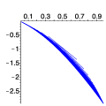
$\frac{1}{\Delta_{n}^{*}(k)}-\frac{1}{S_{1}(\alpha)}$	$\frac{1}{\Delta_{n}^{*}(k)}-\frac{1}{S_{1}(\alpha)}+\frac{T_{1}(\alpha)}{nS_{1}(\alpha)^{2}}$	$\begin{array}[]{l}\frac{1}{\Delta_{n}^{*}(k)}-\frac{1}{S_{1}(\alpha)}+\frac{T_{1}(\alpha)}{nS_{1}(\alpha)^{2}}\\ +\frac{T_{1}(\alpha)^{2}-T_{2}(\alpha)S_{1}(\alpha)}{n^{2}S_{1}(\alpha)^{2}}\end{array}$

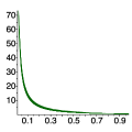
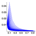
Figure 1: Differences between $\Delta_{n}^{*}(k),\frac{1}{\Delta_{n}^{*}(k)}$ and their asymptotic approximations for $n=2,\dots,50$ (in increasing order of the density of the curves) and $k=1,\dots,n$ (normalized in the unit interval).

$\sum_{1\leq k\leq\lfloor\frac{n}{2}\rfloor}\frac{1}{\Delta_{n}(k)}-\mathbf{E}(X_{n})$	$\sum_{1\leq k\leq\lfloor\frac{n}{2}\rfloor}\frac{1}{\Delta_{n}(k)}-\mathbf{E}(X_{n})-\frac{e}{2}\log n$

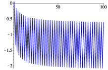
Figure 2: Differences between the exact expected runtime and $\sum_{1\leq k\leq\lfloor\frac{n}{2}\rfloor}\frac{1}{\Delta_{n}(k)}$ without (left) and with (right) the correction term $\frac{e}{2}\log n$.

Conclusions

We have revisited drift analysis for the fundamental problem of bounding the expected runtime of the (1+1) EA on the OneMax problem. Using novel drift theorems involving error bounds, we have bounded the expected runtime when starting from $\lfloor n/2\rfloor$ ones, up to additive terms of logarithmic order; more precisely we have

$$\sum_{k=1}^{\lfloor n/2\rfloor}\frac{1}{\Delta(k)}-\mathord{E}\hskip 1.29167pt\mathord{\left(T\mid X_{0}=\lfloor n/2\rfloor\right)}\in[c_{1}\log n,c_{2}\log n]$$

for explicitly computed constants $c_{1},c_{2}>0$. This for the first time gives an absolute error bound for the expected runtime. Then by standard asymptotic methods, we have found that $\sum_{k=1}^{\lfloor n/2\rfloor}\frac{1}{\Delta(k)}$ overestimates the exact expected runtime by a term ${(e/2)\log n+O(1)}$.

References

• [1] Anne Auger and Benjamin Doerr. Theory of Randomized Search Heuristics – Foundations and Recent Developments. World Scientific Publishing, 2011.
• [2] Francisco Chicano, Andrew M. Sutton, L. Darrell Whitley, and Enrique Alba. Fitness probability distribution of bit-flip mutation. Evolutionary Computation, 23(2):217–248, 2015.
• [3] Benjamin Doerr and Carola Doerr. The impact of random initialization on the runtime of randomized search heuristics. Algorithmica, 75(3):529–553, 2016.
• [4] Benjamin Doerr, Carola Doerr, and Jing Yang. Optimal parameter choices via precise black-box analysis. In Proc. of GECCO ’16, pages 1123–1130. ACM Press, 2016.
• [5] Benjamin Doerr, Mahmoud Fouz, and Carsten Witt. Quasirandom evolutionary algorithms. In Proc. of GECCO ’10, pages 1457–1464. ACM Press, 2010.
• [6] Benjamin Doerr, Mahmoud Fouz, and Carsten Witt. Sharp bounds by probability-generating functions and variable drift. In Proc. of GECCO ’11, pages 2083–2090. ACM Press, 2011.
• [7] Benjamin Doerr, Christian Gießen, Carsten Witt, and Jing Yang. The (1+$\lambda$) evolutionary algorithm with self-adjusting mutation rate. Algorithmica, 81(2):593–631, 2019.
• [8] Benjamin Doerr, Daniel Johannsen, and Carola Winzen. Multiplicative drift analysis. Algorithmica, 64(4):673–697, 2012.
• [9] Stefan Droste, Thomas Jansen, and Ingo Wegener. On the analysis of the (1+1) evolutionary algorithm. Theoretical Computer Science, 276:51–81, 2002.
• [10] Josselin Garnier, Leila Kallel, and Marc Schoenauer. Rigorous hitting times for binary mutations. Evolutionary Computation, 7(2):173–203, 1999.
• [11] Christian Gießen and Carsten Witt. Optimal mutation rates for the (1+$\lambda$) EA on OneMax through asymptotically tight drift analysis. Algorithmica, 80(5):1710–1731, 2018.
• [12] Bruce Hajek. Hitting-time and occupation-time bounds implied by drift analysis with applications. Advances in Applied Probability, 13(3):502–525, 1982.
• [13] Jun He and Xin Yao. Drift analysis and average time complexity of evolutionary algorithms. Artificial Intelligence, 127:57–85, 2001.
• [14] Hsien-Kuei Hwang, Alois Panholzer, Nicolas Rolin, Tsung-Hsi Tsai, and Wei-Mei Chen. Probabilistic analysis of the (1+1)-evolutionary algorithm. CoRR, abs/1409.4955, 2014. http://arxiv.org/abs/1409.4955.
• [15] Hsien-Kuei Hwang, Alois Panholzer, Nicolas Rolin, Tsung-Hsi Tsai, and Wei-Mei Chen. Probabilistic analysis of the (1+1)-evolutionary algorithm. Evolutionary Computation, 26:299–345, 2018.
• [16] Thomas Jansen. Analyzing Evolutionary Algorithms - The Computer Science Perspective. Natural Computing Series. Springer, 2013.
• [17] Daniel Johannsen. Random combinatorial structures and randomized search heuristics. PhD thesis, Universität des Saarlandes, Germany, 2010.
• [18] Timo Kötzing and Martin S. Krejca. First-hitting times for finite state spaces. In Proc. of PPSN ’18, pages 79–91. Springer, 2018.
• [19] Timo Kötzing and Martin S. Krejca. First-hitting times under additive drift. In Proc. of PPSN ’18, pages 92–104. Springer, 2018.
• [20] Per Kristian Lehre. Drift analysis (tutorial). In Companion to GECCO 2012, pages 1239–1258. ACM Press, 2012.
• [21] Per Kristian Lehre and Carsten Witt. Black-box search by unbiased variation. Algorithmica, 64(4):623–642, 2012.
• [22] Per Kristian Lehre and Carsten Witt. General drift analysis with tail bounds. Technical report, 2013. http://arxiv.org/abs/1307.2559.
• [23] Per Kristian Lehre and Carsten Witt. Concentrated hitting times of randomized search heuristics with variable drift. In Proc. of ISAAC ’14, pages 686–697. Springer, 2014.
• [24] Johannes Lengler. Drift analysis. CoRR, abs/1712.00964, 2018. To appear as a book chapter in Theory of Evolutionary Algorithms in Discrete Search Spaces (eds. B. Doerr and F. Neumann), Springer.
• [25] Boris Mitavskiy, Jonathan E. Rowe, and Chris Cannings. Theoretical analysis of local search strategies to optimize network communication subject to preserving the total number of links. International Journal of Intelligent Computing and Cybernetics, 2(2):243–284, 2009.
• [26] Heinz Mühlenbein. How genetic algorithms really work: I. Mutation and hillclimbing. In Proc. of PPSN ’92, pages 15–26. Elsevier, 1992.
• [27] Jonathan E. Rowe and Dirk Sudholt. The choice of the offspring population size in the (1, $\lambda$) evolutionary algorithm. Theoretical Computer Science, 545:20–38, 2014.
• [28] Dirk Sudholt. General lower bounds for the running time of evolutionary algorithms. In Proc. of PPSN ’10, pages 124–133. Springer, 2010.
• [29] Carsten Witt. Tight bounds on the optimization time of a randomized search heuristic on linear functions. Combinatorics, Probability and Computing, 22(2):294–318, 2013.