Higher-order power corrections in a transverse-momentum cut for colour-singlet production at NLO

Abstract

We consider the production of a colourless system at next-to-leading order in the strong coupling constant $\alpha_{\mathchoice{\displaystyle}{\scriptstyle}{\scriptscriptstyle}{\scriptscriptstyle}\rm S}$. We impose a transverse-momentum cutoff, $q_{\mathchoice{\displaystyle}{\scriptstyle}{\scriptscriptstyle}{\scriptscriptstyle}\rm T}^{\mathchoice{\displaystyle}{\scriptstyle}{\scriptscriptstyle}{\scriptscriptstyle}\rm cut}$, on the colourless final state and we compute the power corrections for the inclusive cross section in the cutoff, up to the fourth power.

The study of the dependence of the cross section on $q_{\mathchoice{\displaystyle}{\scriptstyle}{\scriptscriptstyle}{\scriptscriptstyle}\rm T}^{\mathchoice{\displaystyle}{\scriptstyle}{\scriptscriptstyle}{\scriptscriptstyle}\rm cut}$ allows for an understanding of its behaviour at the boundaries of the phase space, giving hints on the structure at all orders in $\alpha_{\mathchoice{\displaystyle}{\scriptstyle}{\scriptscriptstyle}{\scriptscriptstyle}\rm S}$ and on the identification of universal patterns. The knowledge of such power corrections is also a required ingredient in order to reduce the dependence on the transverse-momentum cutoff of the QCD cross sections at higher orders, when the $q_{\mathchoice{\displaystyle}{\scriptstyle}{\scriptscriptstyle}{\scriptscriptstyle}\rm T}$-subtraction method is applied.

We present analytic results for both Drell–Yan vector boson and Higgs boson production in gluon fusion and we illustrate a process-independent procedure for the calculation of the all-order power corrections in the cutoff. In order to show the impact of the power-correction terms, we present selected numerical results and discuss how the residual dependence on $q_{\mathchoice{\displaystyle}{\scriptstyle}{\scriptscriptstyle}{\scriptscriptstyle}\rm T}^{\mathchoice{\displaystyle}{\scriptstyle}{\scriptscriptstyle}{\scriptscriptstyle}\rm cut}$ affects the total cross section for Drell–Yan $Z$ production and Higgs boson production via gluon fusion at the LHC.

1 Introduction

The current precision-physics program at the Large Hadron Collider (LHC) requires Standard Model (SM) theoretical predictions at the highest accuracy. Data belonging to “benchmark” processes, which are measured with the utmost precision at the LHC, need to be tested against theoretical results at the same level of accuracy. This is not only important for the extraction of SM parameters per se, but also for searches of signals of new physics, that can appear as small deviations in kinematic distributions with respect to the SM predictions. Reaching the highest possible level of precision is then the main goal and the calculation of perturbative QCD corrections plays a dominant role in this context.

Until a few years ago, the standard for such calculations was next-to-leading order (NLO) accuracy. In recent years, a continuously-growing number of next-to-next-to-leading order (NNLO) results for many important processes has appeared in the literature, giving birth to the so called “NNLO revolution”. For several “standard candles” processes, the first steps towards the calculation of differential cross sections at N³LO have also been taken (see e.g. Cieri:2018oms ; Dulat:2018bfe ).

The computation of higher-order terms in the perturbative series becomes more involved due to the technical difficulties arising in the evaluation of virtual contributions and to the increasing complexity of the infrared (IR) structure of the real contributions. In order to expose the cancellation of the IR divergences between real and virtual contributions, the knowledge of the behaviour of the scattering amplitudes at the boundaries of the phase space is then a crucial ingredient and it is indeed what is used by the subtraction methods in order to work. These methods can be roughly divided into local and slicing. Among the first, the most extensively used at NLO were proposed in refs. Catani:1996vz ; Frixione:1995ms . As far as the NNLO subtraction methods are concerned, the past few years have witnessed a great activity in their development: the transverse-momentum ($q_{\mathchoice{\displaystyle}{\scriptstyle}{\scriptscriptstyle}{\scriptscriptstyle}\rm T}$) subtraction method Catani:2007vq ; Bozzi:2005wk ; Bonciani:2015sha ; Catani:2019iny , the $N$-jettiness subtraction Boughezal:2015eha ; Gaunt:2015pea , the projection-to-Born Cacciari:2015jma , the residue subtraction Czakon:2011ve ; Boughezal:2011jf and the antenna subtraction method GehrmannDeRidder:2005cm ; Daleo:2006xa ; Currie:2013vh have all been successfully applied to LHC phenomenology. The first application of the $q_{\mathchoice{\displaystyle}{\scriptstyle}{\scriptscriptstyle}{\scriptscriptstyle}\rm T}$-subtraction method to differential cross sections at N³LO was recently proposed in ref. Cieri:2018oms , in the calculation of the rapidity distribution of the Higgs boson.

While a local subtraction is independent of any regularising parameter, slicing methods require the use of a cutoff to separate the different IR regions. Such separation of the phase space introduces instabilities in the numerical evaluation of cross sections and differential distributions Catani:2011qz ; Catani:2018krb ; Grazzini:2017mhc ; Boughezal:2016wmq , and some care has to be taken in order to obtain stable and reliable results.

The knowledge of logarithmic and power-correction terms in the cutoff plays a relevant role in the identification of universal structures, in the development of regularisation prescriptions and in resummation programs Dokshitzer:1978yd ; Dokshitzer:1978hw ; Parisi:1979se ; Curci:1979bg ; Collins:1981uk ; Kodaira:1981nh ; Kodaira:1982az ; Collins:1984kg ; Catani:1988vd ; deFlorian:2000pr ; Alioli:2015toa . According to their behaviour in the zero limit, the cutoff-dependent terms can be classified into logarithmically-divergent or finite contributions, and power-correction terms, that vanish in that limit. In particular, the terms that are singular in the small-cutoff limit are universal and are cancelled by the application of the subtraction methods, while finite and vanishing terms are, in general, process dependent. However, after the subtraction procedure, a residual dependence on the cutoff remains as power corrections. While these terms formally vanish in the null cutoff limit, they give a non-zero numerical contribution for any finite choice of the cutoff.

From a theoretical point of view, the knowledge of the power corrections greatly increases our understanding of the perturbative behaviour of the QCD cross sections, since more non-trivial (universal and non-universal) terms appear. The origin of these terms can be traced back both to the scattering amplitudes, evaluated at phase-space boundaries, and to the phase space itself. Thus, several papers have tackled the study of power corrections in the soft and collinear limits Bern:2014oka ; Larkoski:2014bxa ; Luo:2014wea , while studies in the general framework of fixed-order and threshold-resummed computations have also been performed vanBeekveld:2019cks ; vanBeekveld:2019prq ; DelDuca:2017twk ; Bonocore:2015esa ; Bonocore:2014wua ; Laenen:2010uz ; Laenen:2008ux ; Beneke:2018gvs .

From a practical point of view, the knowledge of the power corrections makes the numerical implementation of a subtraction method more robust, since the power terms weaken the dependence of the final result on the arbitrary cutoff. This is not only valid when the subtraction method is applied to NLO computations, but it is numerically more relevant when applied to higher-order calculation, as pointed out, for example, in the evaluation of NNLO cross sections in refs. Grazzini:2017mhc ; Boughezal:2016wmq .

Power corrections at NLO have been extensively studied in refs. Moult:2016fqy ; Boughezal:2016zws ; Boughezal:2018mvf ; Moult:2017jsg ; Ebert:2018lzn ; Ebert:2018gsn ; Bhattacharya:2018vph ; Campbell:2019gmd ; Moult:2018jjd ; Boughezal:2019ggi in the context of the $N$-jettiness subtraction method, and in refs. Bauer:2000ew ; Bauer:2000yr ; Bauer:2001ct ; Bauer:2001yt ; Bauer:2002aj ; Moult:2019mog within SCET-based subtraction methods. A numerical extraction of power corrections in the context of NNLL’+NNLO calculations was done in $N$-jettiness Alioli:2015toa , and a general discussion in the context of the fixed-order implementation of the $N$-jettiness subtraction can be found in ref. Gaunt:2015pea .

In this paper we consider the production of a colourless system at next-to-leading order in the strong coupling constant $\alpha_{\mathchoice{\displaystyle}{\scriptstyle}{\scriptscriptstyle}{\scriptscriptstyle}\rm S}$. In particular, we discuss Drell–Yan (DY) $V$ production and Higgs boson production in gluon fusion at NLO, in the infinite top-mass limit. We impose a transverse-momentum cutoff, $q_{\mathchoice{\displaystyle}{\scriptstyle}{\scriptscriptstyle}{\scriptscriptstyle}\rm T}^{\mathchoice{\displaystyle}{\scriptstyle}{\scriptscriptstyle}{\scriptscriptstyle}\rm cut}$, on the colourless system and we compute the power corrections in the cutoff, up to order $(q_{\mathchoice{\displaystyle}{\scriptstyle}{\scriptscriptstyle}{\scriptscriptstyle}\rm T}^{\mathchoice{\displaystyle}{\scriptstyle}{\scriptscriptstyle}{\scriptscriptstyle}\rm cut})^{4}$, for the inclusive cross sections. The knowledge of these terms will shed light upon the non-trivial behaviour of cross sections at the boundaries of the phase space, and upon the resummation structure at subleading orders. In addition, it allows to have a better control on the cutoff-dependent terms, when the $q_{\mathchoice{\displaystyle}{\scriptstyle}{\scriptscriptstyle}{\scriptscriptstyle}\rm T}$-subtraction method of ref. Catani:2007vq is applied to the numerical calculation of cross sections, allowing for a use of larger values of the cutoff. We also describe a process-independent procedure that can be used to compute the all-order power corrections in the cutoff.

The outline of this paper is as follows. In sec. 2 we introduce our notation, and we briefly summarize the expressions of the partonic and hadronic cross sections, in a form that is suitable for what follows. In sec. 3 we outline the calculation we have done and in sec. 4 we present and discuss our analytic results for $V$ and $H$ production, along with a study of their numerical impact. We draw our conclusions in sec. 5. We leave to the appendixes all the technical details of our calculation.

2 Kinematics and notation

We briefly introduce the notation used in our theoretical framework and we recall some kinematic details of the calculations presented in this paper.

2.1 Hadronic cross sections

We consider the production of a colourless system $F$ of squared invariant mass $Q^{2}$ plus a coloured system $X$ at a hadron collider

$$h_{1}+h_{2}\rightarrow F+X\,.$$ (1)

We call $S$ the hadronic squared center-of-mass energy and we write the hadronic differential cross section for this process as

$$d\sigma=\sum_{a,b}\int_{\tau}^{1}dx_{1}\int_{\frac{\tau}{x_{1}}}^{1}dx_{2}\,f_{a}\!\left(x_{1}\right)f_{b}\!\left(x_{2}\right)d\hat{\sigma}_{ab}\,,$$ (2)

where

$$\tau=\frac{Q^{2}}{S}\,,$$ (3)

$f_{a/b}$ are the parton densities of the partons $a$ and $b$, in the hadron $h_{1}$ and $h_{2}$ respectively, and $d\hat{\sigma}_{ab}$ is the partonic cross section for the process $a+b\rightarrow F+X$. The dependence on the renormalisation and factorisation scales and on the other kinematic invariants of the process are implicitly assumed.

In appendix A we have collected all the formulae for the calculation of the partonic cross section. Using eqs. (81) and (82), we write the hadronic cross section as

$$\sigma=\sum_{a,b}\int_{\tau}^{1}dx_{1}\int_{\frac{\tau}{x_{1}}}^{1}dx_{2}\,f_{a}\!\left(x_{1}\right)f_{b}\!\left(x_{2}\right)\int dq_{\mathchoice{\displaystyle}{\scriptstyle}{\scriptscriptstyle}{\scriptscriptstyle}\rm T}^{2}\,dz\,\frac{d\hat{\sigma}_{ab}\!\left(q_{\mathchoice{\displaystyle}{\scriptstyle}{\scriptscriptstyle}{\scriptscriptstyle}\rm T},z\right)}{dq_{\mathchoice{\displaystyle}{\scriptstyle}{\scriptscriptstyle}{\scriptscriptstyle}\rm T}^{2}}\,\delta\!\left(\!z-\frac{Q^{2}}{s}\right),$$ (4)

where $s$ is the partonic center-of-mass energy, equal to

$$s=S\,x_{1}\,x_{2}\,.$$ (5)

We have also made explicit the dependence on $z$, the ratio between the squared invariant mass of the system $F$ and the partonic center-of-mass energy, and on $q_{\mathchoice{\displaystyle}{\scriptstyle}{\scriptscriptstyle}{\scriptscriptstyle}\rm T}$, the transverse momentum of the system $F$ with respect to the hadronic beams. Using eqs. (5) and (3) and integrating over $x_{2}$ we obtain

$$\sigma=\sum_{a,b}\tau\int_{\tau}^{1}\frac{dz}{z}\int_{\frac{\tau}{z}}^{1}\frac{dx_{1}}{x_{1}}\,f_{a}\!\left(x_{1}\right)f_{b}\!\left(\frac{\tau}{z\,x_{1}}\right)\frac{1}{z}\int\!dq_{\mathchoice{\displaystyle}{\scriptstyle}{\scriptscriptstyle}{\scriptscriptstyle}\rm T}^{2}\,\frac{d\hat{\sigma}_{ab}\!\left(q_{\mathchoice{\displaystyle}{\scriptstyle}{\scriptscriptstyle}{\scriptscriptstyle}\rm T},z\right)}{dq_{\mathchoice{\displaystyle}{\scriptstyle}{\scriptscriptstyle}{\scriptscriptstyle}\rm T}^{2}}\,.$$ (6)

We then introduce the parton luminosity ${\cal L}_{ab}(y)$ defined by

$${\cal L}_{ab}(y)\equiv\int_{y}^{1}\frac{dx}{x}\,f_{a}\!\left(x\right)f_{b}\!\left(\frac{y}{x}\right),$$ (7)

so that we can finally write

$$\sigma=\sum_{a,b}\tau\int_{\tau}^{1}\frac{dz}{z}\,{\cal L}_{ab}\!\left(\frac{\tau}{z}\right)\frac{1}{z}\int\!dq_{\mathchoice{\displaystyle}{\scriptstyle}{\scriptscriptstyle}{\scriptscriptstyle}\rm T}^{2}\,\frac{d\hat{\sigma}_{ab}\!\left(q_{\mathchoice{\displaystyle}{\scriptstyle}{\scriptscriptstyle}{\scriptscriptstyle}\rm T},z\right)}{dq_{\mathchoice{\displaystyle}{\scriptstyle}{\scriptscriptstyle}{\scriptscriptstyle}\rm T}^{2}}\,.$$ (8)

2.2 Partonic differential cross sections

In this section we recall the formulae for the first-order real corrections to the Drell–Yan production of a weak boson $V$ ($W$ or $Z$) and to the Higgs boson production in gluon fusion, in the infinite top-mass limit.

The partonic cross sections $d\hat{\sigma}_{ab}(q_{\mathchoice{\displaystyle}{\scriptstyle}{\scriptscriptstyle}{\scriptscriptstyle}\rm T},z)/dq_{\mathchoice{\displaystyle}{\scriptstyle}{\scriptscriptstyle}{\scriptscriptstyle}\rm T}^{2}$ in eq. (8) are computable in perturbative QCD as power series in $\alpha_{\mathchoice{\displaystyle}{\scriptstyle}{\scriptscriptstyle}{\scriptscriptstyle}\rm S}$

$$\frac{d\hat{\sigma}_{ab}\!\left(q_{\mathchoice{\displaystyle}{\scriptstyle}{\scriptscriptstyle}{\scriptscriptstyle}\rm T},z\right)}{dq_{\mathchoice{\displaystyle}{\scriptstyle}{\scriptscriptstyle}{\scriptscriptstyle}\rm T}^{2}}=\frac{d\hat{\sigma}^{\mathchoice{\displaystyle}{\scriptstyle}{\scriptscriptstyle}{\scriptscriptstyle}(0)}(q_{\mathchoice{\displaystyle}{\scriptstyle}{\scriptscriptstyle}{\scriptscriptstyle}\rm T},z)}{dq_{\mathchoice{\displaystyle}{\scriptstyle}{\scriptscriptstyle}{\scriptscriptstyle}\rm T}^{2}}+\frac{\alpha_{\mathchoice{\displaystyle}{\scriptstyle}{\scriptscriptstyle}{\scriptscriptstyle}\rm S}}{2\pi}\,\frac{d\hat{\sigma}_{ab}^{\mathchoice{\displaystyle}{\scriptstyle}{\scriptscriptstyle}{\scriptscriptstyle}(1)}(q_{\mathchoice{\displaystyle}{\scriptstyle}{\scriptscriptstyle}{\scriptscriptstyle}\rm T},z)}{dq_{\mathchoice{\displaystyle}{\scriptstyle}{\scriptscriptstyle}{\scriptscriptstyle}\rm T}^{2}}+\ldots$$ (9)

The Born contribution ${d\hat{\sigma}^{\mathchoice{\displaystyle}{\scriptstyle}{\scriptscriptstyle}{\scriptscriptstyle}(0)}(q_{\mathchoice{\displaystyle}{\scriptstyle}{\scriptscriptstyle}{\scriptscriptstyle}\rm T},z)}/{dq_{\mathchoice{\displaystyle}{\scriptstyle}{\scriptscriptstyle}{\scriptscriptstyle}\rm T}^{2}}$ and the virtual contributions to ${d\hat{\sigma}_{ab}^{\mathchoice{\displaystyle}{\scriptstyle}{\scriptscriptstyle}{\scriptscriptstyle}(1)}(q_{\mathchoice{\displaystyle}{\scriptstyle}{\scriptscriptstyle}{\scriptscriptstyle}\rm T},z)}/{dq_{\mathchoice{\displaystyle}{\scriptstyle}{\scriptscriptstyle}{\scriptscriptstyle}\rm T}^{2}}$ are proportional to $\delta(q_{\mathchoice{\displaystyle}{\scriptstyle}{\scriptscriptstyle}{\scriptscriptstyle}\rm T})$.

Applying the formulae detailed in appendix A, with a little abuse of notation, we can write the partonic differential cross sections for the real corrections to $V$ and $H$ production as

$\boldsymbol{V}$ production

• $q(\bar{q})+g\rightarrow V+q(\bar{q})$

  $$\frac{d\hat{\sigma}_{qg}^{\mathchoice{\displaystyle}{\scriptstyle}{\scriptscriptstyle}{\scriptscriptstyle}(1)}(q_{\mathchoice{\displaystyle}{\scriptstyle}{\scriptscriptstyle}{\scriptscriptstyle}\rm T},z)}{dq_{\mathchoice{\displaystyle}{\scriptstyle}{\scriptscriptstyle}{\scriptscriptstyle}\rm T}^{2}}=\sigma_{qq}^{\mathchoice{\displaystyle}{\scriptstyle}{\scriptscriptstyle}{\scriptscriptstyle}(0)}\,T_{\mathchoice{\displaystyle}{\scriptstyle}{\scriptscriptstyle}{\scriptscriptstyle}\rm R}\,z\,\frac{z\,(1+3z)\,{\displaystyle\frac{q_{\mathchoice{\displaystyle}{\scriptstyle}{\scriptscriptstyle}{\scriptscriptstyle}\rm T}^{2}}{Q^{2}}}+(1-z)\,p_{qg}(z)}{\sqrt{(1-z)^{2}-4z\,{\displaystyle\frac{q_{\mathchoice{\displaystyle}{\scriptstyle}{\scriptscriptstyle}{\scriptscriptstyle}\rm T}^{2}}{Q^{2}}}}}\,\frac{1}{q_{\mathchoice{\displaystyle}{\scriptstyle}{\scriptscriptstyle}{\scriptscriptstyle}\rm T}^{2}}\,,$$ (10)

• $q+\bar{q}\rightarrow V+g$

  $$\frac{d\hat{\sigma}_{q\bar{q}}^{\mathchoice{\displaystyle}{\scriptstyle}{\scriptscriptstyle}{\scriptscriptstyle}(1)}(q_{\mathchoice{\displaystyle}{\scriptstyle}{\scriptscriptstyle}{\scriptscriptstyle}\rm T},z)}{dq_{\mathchoice{\displaystyle}{\scriptstyle}{\scriptscriptstyle}{\scriptscriptstyle}\rm T}^{2}}=\sigma_{qq}^{\mathchoice{\displaystyle}{\scriptstyle}{\scriptscriptstyle}{\scriptscriptstyle}(0)}\,C_{\mathchoice{\displaystyle}{\scriptstyle}{\scriptscriptstyle}{\scriptscriptstyle}\rm F}\,z\,\frac{-4z\,{\displaystyle\frac{q_{\mathchoice{\displaystyle}{\scriptstyle}{\scriptscriptstyle}{\scriptscriptstyle}\rm T}^{2}}{Q^{2}}}+2\,(1-z)\,\hat{p}_{qq}(z)}{\sqrt{(1-z)^{2}-4z\,{\displaystyle\frac{q_{\mathchoice{\displaystyle}{\scriptstyle}{\scriptscriptstyle}{\scriptscriptstyle}\rm T}^{2}}{Q^{2}}}}}\,\frac{1}{q_{\mathchoice{\displaystyle}{\scriptstyle}{\scriptscriptstyle}{\scriptscriptstyle}\rm T}^{2}}\,,$$ (11)

where

$$\sigma_{qq}^{\mathchoice{\displaystyle}{\scriptstyle}{\scriptscriptstyle}{\scriptscriptstyle}(0)}=\frac{\pi}{N_{\rm c}}\,\frac{g^{2}\left(g_{v}^{2}+g_{a}^{2}\right)}{c_{\rm\mathchoice{\displaystyle}{\scriptstyle}{\scriptscriptstyle}{\scriptscriptstyle}W}^{2}}\frac{1}{Q^{2}}$$ (12)

is the Born-level cross section for the process $q\bar{q}\rightarrow V$, with $c_{\rm\mathchoice{\displaystyle}{\scriptstyle}{\scriptscriptstyle}{\scriptscriptstyle}W}$ the cosine of the weak angle and $g$, $g_{v}$, $g_{a}$ the weak, the vector and the axial coupling, respectively. With $N_{\rm c}$ we denote the number of colours, $C_{\mathchoice{\displaystyle}{\scriptstyle}{\scriptscriptstyle}{\scriptscriptstyle}\rm F}=\left(N_{\rm c}^{2}-1\right)/2N_{\rm c}=4/3$ and $T_{\mathchoice{\displaystyle}{\scriptstyle}{\scriptscriptstyle}{\scriptscriptstyle}\rm R}=1/2$. For $W$ production, the flavours of the quarks in eqs. (10)–(12) are different, and the corresponding Cabibbo–Kobayashi–Maskawa matrix element has to be included in eq. (12). The expression of the Altarelli–Parisi splitting functions $p_{qg}(z)$ and $\hat{p}_{qq}(z)$ are given in appendix D.

$\boldsymbol{H}$ production

• $g+q(\bar{q})\rightarrow H+q(\bar{q})$

  $$\frac{d\hat{\sigma}_{gq}^{\mathchoice{\displaystyle}{\scriptstyle}{\scriptscriptstyle}{\scriptscriptstyle}(1)}(q_{\mathchoice{\displaystyle}{\scriptstyle}{\scriptscriptstyle}{\scriptscriptstyle}\rm T},z)}{dq_{\mathchoice{\displaystyle}{\scriptstyle}{\scriptscriptstyle}{\scriptscriptstyle}\rm T}^{2}}=\sigma_{gg}^{\mathchoice{\displaystyle}{\scriptstyle}{\scriptscriptstyle}{\scriptscriptstyle}(0)}\,C_{\mathchoice{\displaystyle}{\scriptstyle}{\scriptscriptstyle}{\scriptscriptstyle}\rm F}\,z\,\frac{-3\,(1-z)\,{\displaystyle\frac{q_{\mathchoice{\displaystyle}{\scriptstyle}{\scriptscriptstyle}{\scriptscriptstyle}\rm T}^{2}}{Q^{2}}}+(1-z)\,p_{gq}(z)}{\sqrt{(1-z)^{2}-4z\,{\displaystyle\frac{q_{\mathchoice{\displaystyle}{\scriptstyle}{\scriptscriptstyle}{\scriptscriptstyle}\rm T}^{2}}{Q^{2}}}}}\,\frac{1}{q_{\mathchoice{\displaystyle}{\scriptstyle}{\scriptscriptstyle}{\scriptscriptstyle}\rm T}^{2}}\,,$$ (13)

• $g+g\rightarrow H+g$

  $$\frac{d\hat{\sigma}_{gg}^{\mathchoice{\displaystyle}{\scriptstyle}{\scriptscriptstyle}{\scriptscriptstyle}(1)}(q_{\mathchoice{\displaystyle}{\scriptstyle}{\scriptscriptstyle}{\scriptscriptstyle}\rm T},z)}{dq_{\mathchoice{\displaystyle}{\scriptstyle}{\scriptscriptstyle}{\scriptscriptstyle}\rm T}^{2}}=\sigma_{gg}^{\mathchoice{\displaystyle}{\scriptstyle}{\scriptscriptstyle}{\scriptscriptstyle}(0)}\,C_{\mathchoice{\displaystyle}{\scriptstyle}{\scriptscriptstyle}{\scriptscriptstyle}\rm A}\,z\,\frac{4z\left({\displaystyle\frac{q_{\mathchoice{\displaystyle}{\scriptstyle}{\scriptscriptstyle}{\scriptscriptstyle}\rm T}^{2}}{Q^{2}}}\right)^{\!\!2}-8\,(1-z)^{2}\,{\displaystyle\frac{q_{\mathchoice{\displaystyle}{\scriptstyle}{\scriptscriptstyle}{\scriptscriptstyle}\rm T}^{2}}{Q^{2}}}+2\,(1-z)\,\hat{p}_{gg}(z)}{\sqrt{(1-z)^{2}-4z\,{\displaystyle\frac{q_{\mathchoice{\displaystyle}{\scriptstyle}{\scriptscriptstyle}{\scriptscriptstyle}\rm T}^{2}}{Q^{2}}}}}\,\frac{1}{q_{\mathchoice{\displaystyle}{\scriptstyle}{\scriptscriptstyle}{\scriptscriptstyle}\rm T}^{2}}\,,\phantom{aaa}$$ (14)

where

$$\sigma_{gg}^{\mathchoice{\displaystyle}{\scriptstyle}{\scriptscriptstyle}{\scriptscriptstyle}(0)}=\frac{\alpha_{\mathchoice{\displaystyle}{\scriptstyle}{\scriptscriptstyle}{\scriptscriptstyle}\rm S}^{2}}{72\pi}\,\frac{1}{N_{\rm c}^{2}-1}\,\frac{1}{v^{2}}$$ (15)

is the Born-level cross section for the process $gg\rightarrow H$, with $v$ the Higgs vacuum expectation value and $C_{\mathchoice{\displaystyle}{\scriptstyle}{\scriptscriptstyle}{\scriptscriptstyle}\rm A}=N_{\rm c}=3$. The expression of the Altarelli–Parisi splitting functions $p_{gq}(z)$ and $\hat{p}_{gg}(z)$ are given in appendix D.

We notice that the terms proportional to the Altarelli–Parisi splitting functions in eqs. (10)–(14) embody in a single expression the whole infrared behaviour of the amplitudes, i.e. their soft and collinear limits. The structure of these terms was derived in a completely general form, from the universal behaviour of the scattering amplitudes in those limits, in ref. deFlorian:2001zd .

3 Description of the calculation

In the small-$q_{\mathchoice{\displaystyle}{\scriptstyle}{\scriptscriptstyle}{\scriptscriptstyle}\rm T}$ region, i.e. $q_{\mathchoice{\displaystyle}{\scriptstyle}{\scriptscriptstyle}{\scriptscriptstyle}\rm T}\ll Q$, the real contribution to the perturbative cross sections of eqs. (10)–(14) contains well-known logarithmically-enhanced terms that are singular in the $q_{\mathchoice{\displaystyle}{\scriptstyle}{\scriptscriptstyle}{\scriptscriptstyle}\rm T}\rightarrow 0$ limit Dokshitzer:1978yd ; Dokshitzer:1978hw ; Parisi:1979se ; Curci:1979bg ; Collins:1981uk ; Kodaira:1981nh ; Kodaira:1982az ; Collins:1984kg ; Catani:1988vd ; deFlorian:2000pr . In the context of inclusive NLO fixed-order calculations, the logarithmic terms are cancelled when using the subtraction prescriptions. For more exclusive quantities, such as the transverse-momentum distribution of the colourless system, the same logarithmic terms need to be resummed at all orders in the strong coupling constant to produce reliable results. Although our studies are of value in the context of the transverse-momentum resummation, here we limit ourselves to the case of inclusive fixed-order predictions at NLO, leaving the resummation program to future investigations. In this paper we compute power-correction terms to the cross section that, although vanishing in the small-$q_{\mathchoice{\displaystyle}{\scriptstyle}{\scriptscriptstyle}{\scriptscriptstyle}\rm T}$ limit, may give a sizable numerical contribution when using a slicing subtraction method.

To explicitly present the perturbative structure of these terms at small $q_{\mathchoice{\displaystyle}{\scriptstyle}{\scriptscriptstyle}{\scriptscriptstyle}\rm T}$, it is customary in the literature deFlorian:2001zd ; Ebert:2018lzn to compute the following cumulative partonic cross section, integrating the differential cross section in the range $0\leq q_{\mathchoice{\displaystyle}{\scriptstyle}{\scriptscriptstyle}{\scriptscriptstyle}\rm T}\leq q_{\mathchoice{\displaystyle}{\scriptstyle}{\scriptscriptstyle}{\scriptscriptstyle}\rm T}^{\mathchoice{\displaystyle}{\scriptstyle}{\scriptscriptstyle}{\scriptscriptstyle}\rm cut}$,

$$\hat{\sigma}_{ab}^{\mathchoice{\displaystyle}{\scriptstyle}{\scriptscriptstyle}{\scriptscriptstyle}<}(z)\equiv\int_{0}^{\left(q_{\mathchoice{\displaystyle}{\scriptstyle}{\scriptscriptstyle}{\scriptscriptstyle}\rm T}^{\mathchoice{\displaystyle}{\scriptstyle}{\scriptscriptstyle}{\scriptscriptstyle}\rm cut}\right)^{2}}\!\!dq_{\mathchoice{\displaystyle}{\scriptstyle}{\scriptscriptstyle}{\scriptscriptstyle}\rm T}^{2}\,\frac{d\hat{\sigma}_{ab}(q_{\mathchoice{\displaystyle}{\scriptstyle}{\scriptscriptstyle}{\scriptscriptstyle}\rm T},z)}{dq_{\mathchoice{\displaystyle}{\scriptstyle}{\scriptscriptstyle}{\scriptscriptstyle}\rm T}^{2}}.$$ (16)

The cross section in eq. (16) receives contributions from the Born and the virtual terms, both proportional to $\delta(q_{\mathchoice{\displaystyle}{\scriptstyle}{\scriptscriptstyle}{\scriptscriptstyle}\rm T})$, and from the part of the real amplitude that describes the production of the $F$ system with transverse momentum less than $q_{\mathchoice{\displaystyle}{\scriptstyle}{\scriptscriptstyle}{\scriptscriptstyle}\rm T}^{\mathchoice{\displaystyle}{\scriptstyle}{\scriptscriptstyle}{\scriptscriptstyle}\rm cut}$. The virtual and real contributions are separately divergent and are typically regularised in dimensional regularisation. Since the total partonic cross section is finite and analytically known for the processes under study, following what was done in refs. Catani:2011kr ; Catani:2012qa , we compute the above integral as

$$\hat{\sigma}_{ab}^{\mathchoice{\displaystyle}{\scriptstyle}{\scriptscriptstyle}{\scriptscriptstyle}<}(z)=\hat{\sigma}^{\rm\mathchoice{\displaystyle}{\scriptstyle}{\scriptscriptstyle}{\scriptscriptstyle}tot}_{ab}(z)-\hat{\sigma}_{ab}^{\mathchoice{\displaystyle}{\scriptstyle}{\scriptscriptstyle}{\scriptscriptstyle}>}(z)\,,$$ (17)

with

$$\hat{\sigma}^{\rm\mathchoice{\displaystyle}{\scriptstyle}{\scriptscriptstyle}{\scriptscriptstyle}tot}_{ab}(z) = \int_{0}^{\left(q_{\mathchoice{\displaystyle}{\scriptstyle}{\scriptscriptstyle}{\scriptscriptstyle}\rm T}^{\mathchoice{\displaystyle}{\scriptstyle}{\scriptscriptstyle}{\scriptscriptstyle}\rm max}\right)^{2}}\!\!dq_{\mathchoice{\displaystyle}{\scriptstyle}{\scriptscriptstyle}{\scriptscriptstyle}\rm T}^{2}\,\frac{d\hat{\sigma}_{ab}(q_{\mathchoice{\displaystyle}{\scriptstyle}{\scriptscriptstyle}{\scriptscriptstyle}\rm T},z)}{dq_{\mathchoice{\displaystyle}{\scriptstyle}{\scriptscriptstyle}{\scriptscriptstyle}\rm T}^{2}}\,,$$ (18)

$$\hat{\sigma}_{ab}^{\mathchoice{\displaystyle}{\scriptstyle}{\scriptscriptstyle}{\scriptscriptstyle}>}(z) = \int_{\left(q_{\mathchoice{\displaystyle}{\scriptstyle}{\scriptscriptstyle}{\scriptscriptstyle}\rm T}^{\mathchoice{\displaystyle}{\scriptstyle}{\scriptscriptstyle}{\scriptscriptstyle}\rm cut}\right)^{2}}^{\left(q_{\mathchoice{\displaystyle}{\scriptstyle}{\scriptscriptstyle}{\scriptscriptstyle}\rm T}^{\mathchoice{\displaystyle}{\scriptstyle}{\scriptscriptstyle}{\scriptscriptstyle}\rm max}\right)^{2}}\!\!dq_{\mathchoice{\displaystyle}{\scriptstyle}{\scriptscriptstyle}{\scriptscriptstyle}\rm T}^{2}\,\frac{d\hat{\sigma}_{ab}(q_{\mathchoice{\displaystyle}{\scriptstyle}{\scriptscriptstyle}{\scriptscriptstyle}\rm T},z)}{dq_{\mathchoice{\displaystyle}{\scriptstyle}{\scriptscriptstyle}{\scriptscriptstyle}\rm T}^{2}}\,,$$ (19)

where $q_{\mathchoice{\displaystyle}{\scriptstyle}{\scriptscriptstyle}{\scriptscriptstyle}\rm T}^{\mathchoice{\displaystyle}{\scriptstyle}{\scriptscriptstyle}{\scriptscriptstyle}\rm max}$ is the maximum transverse momentum allowed by the kinematics, $\hat{\sigma}^{\rm\mathchoice{\displaystyle}{\scriptstyle}{\scriptscriptstyle}{\scriptscriptstyle}tot}_{ab}(z)$ is the total partonic cross section and $\hat{\sigma}_{ab}^{\mathchoice{\displaystyle}{\scriptstyle}{\scriptscriptstyle}{\scriptscriptstyle}>}(z)$ is the partonic cross section integrated above $q_{\mathchoice{\displaystyle}{\scriptstyle}{\scriptscriptstyle}{\scriptscriptstyle}\rm T}^{\mathchoice{\displaystyle}{\scriptstyle}{\scriptscriptstyle}{\scriptscriptstyle}\rm cut}$. The advantage of using eq. (17) is that the partonic cross section integrated in the range $0\leq q_{\mathchoice{\displaystyle}{\scriptstyle}{\scriptscriptstyle}{\scriptscriptstyle}\rm T}\leq q_{\mathchoice{\displaystyle}{\scriptstyle}{\scriptscriptstyle}{\scriptscriptstyle}\rm T}^{\mathchoice{\displaystyle}{\scriptstyle}{\scriptscriptstyle}{\scriptscriptstyle}\rm cut}$ is obtained as difference of the total cross section (formally free from any dependence on $q_{\mathchoice{\displaystyle}{\scriptstyle}{\scriptscriptstyle}{\scriptscriptstyle}\rm T}^{\mathchoice{\displaystyle}{\scriptstyle}{\scriptscriptstyle}{\scriptscriptstyle}\rm cut}$) and the partonic cross section integrated in the range above $q_{\mathchoice{\displaystyle}{\scriptstyle}{\scriptscriptstyle}{\scriptscriptstyle}\rm T}^{\mathchoice{\displaystyle}{\scriptstyle}{\scriptscriptstyle}{\scriptscriptstyle}\rm cut}$ of eq. (19). Since $q_{\mathchoice{\displaystyle}{\scriptstyle}{\scriptscriptstyle}{\scriptscriptstyle}\rm T}>q_{\mathchoice{\displaystyle}{\scriptstyle}{\scriptscriptstyle}{\scriptscriptstyle}\rm T}^{\mathchoice{\displaystyle}{\scriptstyle}{\scriptscriptstyle}{\scriptscriptstyle}\rm cut}>0$, the last integration can be performed in four space-time dimensions, with no further use of dimensional regularisation. In refs. Catani:2011kr ; Catani:2012qa the computation of the cumulative cross section was performed in the limit $q_{\mathchoice{\displaystyle}{\scriptstyle}{\scriptscriptstyle}{\scriptscriptstyle}\rm T}^{\mathchoice{\displaystyle}{\scriptstyle}{\scriptscriptstyle}{\scriptscriptstyle}\rm cut}\ll Q$, neglecting terms of $\mathcal{O}\!\left((q_{\mathchoice{\displaystyle}{\scriptstyle}{\scriptscriptstyle}{\scriptscriptstyle}\rm T}^{\mathchoice{\displaystyle}{\scriptstyle}{\scriptscriptstyle}{\scriptscriptstyle}\rm cut})^{2}\right)$ on the right-hand side of eq. (17). In this paper, we compute these terms up to $\mathcal{O}\!\left((q_{\mathchoice{\displaystyle}{\scriptstyle}{\scriptscriptstyle}{\scriptscriptstyle}\rm T}^{\mathchoice{\displaystyle}{\scriptstyle}{\scriptscriptstyle}{\scriptscriptstyle}\rm cut})^{4}\right)$ included.

3.1 $\boldsymbol{q_{\mathchoice{\displaystyle}{\scriptstyle}{\scriptscriptstyle}{\scriptscriptstyle}\rm T}}$-integrated partonic cross sections

In this section we present the results for the partonic cross section in eq. (19), integrated in $q_{\mathchoice{\displaystyle}{\scriptstyle}{\scriptscriptstyle}{\scriptscriptstyle}\rm T}$, from an arbitrary value $q_{\mathchoice{\displaystyle}{\scriptstyle}{\scriptscriptstyle}{\scriptscriptstyle}\rm T}^{\mathchoice{\displaystyle}{\scriptstyle}{\scriptscriptstyle}{\scriptscriptstyle}\rm cut}$ up to the maximum transverse momentum $q_{\mathchoice{\displaystyle}{\scriptstyle}{\scriptscriptstyle}{\scriptscriptstyle}\rm T}^{\mathchoice{\displaystyle}{\scriptstyle}{\scriptscriptstyle}{\scriptscriptstyle}\rm max}$ allowed by the kinematics of the event, given by

$$\left(q_{\mathchoice{\displaystyle}{\scriptstyle}{\scriptscriptstyle}{\scriptscriptstyle}\rm T}^{\mathchoice{\displaystyle}{\scriptstyle}{\scriptscriptstyle}{\scriptscriptstyle}\rm max}\right)^{2}=Q^{2}\,\frac{(1-z)^{2}}{4\,z}\,,$$ (20)

at a fixed value of $z$. The integrations are straightforward and do not need any dedicated comment. To lighten up the notation, we introduce the dimensionless quantity

$$a\equiv\frac{\left(q_{\mathchoice{\displaystyle}{\scriptstyle}{\scriptscriptstyle}{\scriptscriptstyle}\rm T}^{\mathchoice{\displaystyle}{\scriptstyle}{\scriptscriptstyle}{\scriptscriptstyle}\rm cut}\right)^{2}}{Q^{2}}\,,$$ (21)

that will be our expansion parameter in the rest of the paper, and we define

$$\pi_{\mathchoice{\displaystyle}{\scriptstyle}{\scriptscriptstyle}{\scriptscriptstyle}\rm T}^{2}\equiv\frac{4az}{(1-z)^{2}}\,,$$ (22)

that will allow us to write the upcoming differential cross sections in a more compact form.

$\boldsymbol{V}$ production

• $q(\bar{q})+g\rightarrow V+q(\bar{q})$

  $$\hat{\sigma}_{qg}^{\mathchoice{\displaystyle}{\scriptstyle}{\scriptscriptstyle}{\scriptscriptstyle}>(1)}(z) = \int_{\left(q_{\mathchoice{\displaystyle}{\scriptstyle}{\scriptscriptstyle}{\scriptscriptstyle}\rm T}^{\mathchoice{\displaystyle}{\scriptstyle}{\scriptscriptstyle}{\scriptscriptstyle}\rm cut}\right)^{2}}^{\left(q_{\mathchoice{\displaystyle}{\scriptstyle}{\scriptscriptstyle}{\scriptscriptstyle}\rm T}^{\mathchoice{\displaystyle}{\scriptstyle}{\scriptscriptstyle}{\scriptscriptstyle}\rm max}\right)^{2}}\!\!dq_{\mathchoice{\displaystyle}{\scriptstyle}{\scriptscriptstyle}{\scriptscriptstyle}\rm T}^{2}\,\frac{d\hat{\sigma}_{qg}^{\mathchoice{\displaystyle}{\scriptstyle}{\scriptscriptstyle}{\scriptscriptstyle}(1)}(q_{\mathchoice{\displaystyle}{\scriptstyle}{\scriptscriptstyle}{\scriptscriptstyle}\rm T},z)}{dq_{\mathchoice{\displaystyle}{\scriptstyle}{\scriptscriptstyle}{\scriptscriptstyle}\rm T}^{2}}$$ (23)

  $$= \sigma_{qq}^{\mathchoice{\displaystyle}{\scriptstyle}{\scriptscriptstyle}{\scriptscriptstyle}(0)}\,T_{\mathchoice{\displaystyle}{\scriptstyle}{\scriptscriptstyle}{\scriptscriptstyle}\rm R}\,z\left\{\frac{1}{2}(1+3z)(1-z)\,\sqrt{1-\frac{4az}{(1-z)^{2}}}\right.$$

  $$\hskip 19.91684pt\left.+\,p_{qg}(z)\!\left[-\log{\frac{az}{(1-z)^{2}}}+2\log\frac{1}{2}\left(\sqrt{1-\frac{4az}{(1-z)^{2}}}+1\right)\right]\right\}$$

  $$= \sigma_{qq}^{\mathchoice{\displaystyle}{\scriptstyle}{\scriptscriptstyle}{\scriptscriptstyle}(0)}\,T_{\mathchoice{\displaystyle}{\scriptstyle}{\scriptscriptstyle}{\scriptscriptstyle}\rm R}\,z\left\{\frac{1}{2}(1+3z)(1-z)\,\sqrt{1-\pi_{\mathchoice{\displaystyle}{\scriptstyle}{\scriptscriptstyle}{\scriptscriptstyle}\rm T}^{2}}+p_{qg}(z)\log\frac{1+\sqrt{1-\pi_{\mathchoice{\displaystyle}{\scriptstyle}{\scriptscriptstyle}{\scriptscriptstyle}\rm T}^{2}}}{1-\sqrt{1-\pi_{\mathchoice{\displaystyle}{\scriptstyle}{\scriptscriptstyle}{\scriptscriptstyle}\rm T}^{2}}}\right\}\!,\phantom{aaaa}$$

• $q+\bar{q}\rightarrow V+g$

  $$\hat{\sigma}_{q\bar{q}}^{\mathchoice{\displaystyle}{\scriptstyle}{\scriptscriptstyle}{\scriptscriptstyle}>(1)}(z) = \int_{\left(q_{\mathchoice{\displaystyle}{\scriptstyle}{\scriptscriptstyle}{\scriptscriptstyle}\rm T}^{\mathchoice{\displaystyle}{\scriptstyle}{\scriptscriptstyle}{\scriptscriptstyle}\rm cut}\right)^{2}}^{\left(q_{\mathchoice{\displaystyle}{\scriptstyle}{\scriptscriptstyle}{\scriptscriptstyle}\rm T}^{\mathchoice{\displaystyle}{\scriptstyle}{\scriptscriptstyle}{\scriptscriptstyle}\rm max}\right)^{2}}\!\!\frac{d\hat{\sigma}_{q\bar{q}}^{\mathchoice{\displaystyle}{\scriptstyle}{\scriptscriptstyle}{\scriptscriptstyle}(1)}(q_{\mathchoice{\displaystyle}{\scriptstyle}{\scriptscriptstyle}{\scriptscriptstyle}\rm T},z)}{dq_{\mathchoice{\displaystyle}{\scriptstyle}{\scriptscriptstyle}{\scriptscriptstyle}\rm T}^{2}}$$ (24)

  $$= \sigma_{qq}^{\mathchoice{\displaystyle}{\scriptstyle}{\scriptscriptstyle}{\scriptscriptstyle}(0)}\,C_{\mathchoice{\displaystyle}{\scriptstyle}{\scriptscriptstyle}{\scriptscriptstyle}\rm F}\,z\left\{-2\,(1-z)\,\sqrt{1-\frac{4az}{(1-z)^{2}}}\right.$$

  $$\hskip 19.91684pt\left.{}+2\,\hat{p}_{qq}(z)\!\left[-\log\frac{az}{(1-z)^{2}}+2\log\frac{1}{2}\left(\sqrt{1-\frac{4az}{(1-z)^{2}}}+1\right)\right]\!\right\}\phantom{aaaaaa}$$

  $$= \sigma_{qq}^{\mathchoice{\displaystyle}{\scriptstyle}{\scriptscriptstyle}{\scriptscriptstyle}(0)}\,C_{\mathchoice{\displaystyle}{\scriptstyle}{\scriptscriptstyle}{\scriptscriptstyle}\rm F}\,z\left\{-2\,(1-z)\,\sqrt{1-\pi_{\mathchoice{\displaystyle}{\scriptstyle}{\scriptscriptstyle}{\scriptscriptstyle}\rm T}^{2}}+2\,\hat{p}_{qq}(z)\log\frac{1+\sqrt{1-\pi_{\mathchoice{\displaystyle}{\scriptstyle}{\scriptscriptstyle}{\scriptscriptstyle}\rm T}^{2}}}{1-\sqrt{1-\pi_{\mathchoice{\displaystyle}{\scriptstyle}{\scriptscriptstyle}{\scriptscriptstyle}\rm T}^{2}}}\right\}\!.$$

$\boldsymbol{H}$ production

• $g+q(\bar{q})\rightarrow H+q(\bar{q})$

  $$\hat{\sigma}_{gq}^{\mathchoice{\displaystyle}{\scriptstyle}{\scriptscriptstyle}{\scriptscriptstyle}>(1)}(z) = \int_{\left(q_{\mathchoice{\displaystyle}{\scriptstyle}{\scriptscriptstyle}{\scriptscriptstyle}\rm T}^{\mathchoice{\displaystyle}{\scriptstyle}{\scriptscriptstyle}{\scriptscriptstyle}\rm cut}\right)^{2}}^{\left(q_{\mathchoice{\displaystyle}{\scriptstyle}{\scriptscriptstyle}{\scriptscriptstyle}\rm T}^{\mathchoice{\displaystyle}{\scriptstyle}{\scriptscriptstyle}{\scriptscriptstyle}\rm max}\right)^{2}}\!\!\frac{d\hat{\sigma}_{gq}^{\mathchoice{\displaystyle}{\scriptstyle}{\scriptscriptstyle}{\scriptscriptstyle}(1)}(q_{\mathchoice{\displaystyle}{\scriptstyle}{\scriptscriptstyle}{\scriptscriptstyle}\rm T},z)}{dq_{\mathchoice{\displaystyle}{\scriptstyle}{\scriptscriptstyle}{\scriptscriptstyle}\rm T}^{2}}$$ (25)

  $$= \sigma_{gg}^{\mathchoice{\displaystyle}{\scriptstyle}{\scriptscriptstyle}{\scriptscriptstyle}(0)}\,C_{\mathchoice{\displaystyle}{\scriptstyle}{\scriptscriptstyle}{\scriptscriptstyle}\rm F}\,z\left\{-\frac{3(1-z)^{2}}{2z}\,\sqrt{1-\frac{4az}{(1-z)^{2}}}\right.$$

  $$\hskip 19.91684pt\left.{}+p_{gq}(z)\!\left[-\log\frac{az}{(1-z)^{2}}+2\log\frac{1}{2}\left(\sqrt{1-\frac{4az}{(1-z)^{2}}}+1\right)\right]\right\}\phantom{aaaaa}$$

  $$= \sigma_{gg}^{\mathchoice{\displaystyle}{\scriptstyle}{\scriptscriptstyle}{\scriptscriptstyle}(0)}\,C_{\mathchoice{\displaystyle}{\scriptstyle}{\scriptscriptstyle}{\scriptscriptstyle}\rm F}\,z\left\{-\frac{3(1-z)^{2}}{2z}\,\sqrt{1-\pi_{\mathchoice{\displaystyle}{\scriptstyle}{\scriptscriptstyle}{\scriptscriptstyle}\rm T}^{2}}+p_{gq}(z)\log\frac{1+\sqrt{1-\pi_{\mathchoice{\displaystyle}{\scriptstyle}{\scriptscriptstyle}{\scriptscriptstyle}\rm T}^{2}}}{1-\sqrt{1-\pi_{\mathchoice{\displaystyle}{\scriptstyle}{\scriptscriptstyle}{\scriptscriptstyle}\rm T}^{2}}}\right\}\!,$$

• $g+g\rightarrow H+g$

  $$\hat{\sigma}_{gg}^{\mathchoice{\displaystyle}{\scriptstyle}{\scriptscriptstyle}{\scriptscriptstyle}>(1)}(z) = \int_{\left(q_{\mathchoice{\displaystyle}{\scriptstyle}{\scriptscriptstyle}{\scriptscriptstyle}\rm T}^{\mathchoice{\displaystyle}{\scriptstyle}{\scriptscriptstyle}{\scriptscriptstyle}\rm cut}\right)^{2}}^{\left(q_{\mathchoice{\displaystyle}{\scriptstyle}{\scriptscriptstyle}{\scriptscriptstyle}\rm T}^{\mathchoice{\displaystyle}{\scriptstyle}{\scriptscriptstyle}{\scriptscriptstyle}\rm max}\right)^{2}}\!\!\frac{d\hat{\sigma}_{gg}^{\mathchoice{\displaystyle}{\scriptstyle}{\scriptscriptstyle}{\scriptscriptstyle}(1)}(q_{\mathchoice{\displaystyle}{\scriptstyle}{\scriptscriptstyle}{\scriptscriptstyle}\rm T},z)}{dq_{\mathchoice{\displaystyle}{\scriptstyle}{\scriptscriptstyle}{\scriptscriptstyle}\rm T}^{2}}$$

  $$= \sigma_{gg}^{\mathchoice{\displaystyle}{\scriptstyle}{\scriptscriptstyle}{\scriptscriptstyle}(0)}\,C_{\mathchoice{\displaystyle}{\scriptstyle}{\scriptscriptstyle}{\scriptscriptstyle}\rm A}\,z\left\{-\frac{4(1-z)^{3}}{z}\,\sqrt{1-\frac{4az}{(1-z)^{2}}}\right.$$

  $$\hskip 19.91684pt{}+4\,z\left[\frac{1-z}{2z}\,\frac{(1-z)^{2}}{6z}\,\sqrt{1-\frac{4az}{(1-z)^{2}}}\,\left(1+\frac{2az}{(1-z)^{2}}\right)\right]$$

  $$\hskip 19.91684pt{}\left.{}+2\,\hat{p}_{gg}(z)\left[-\log{\frac{az}{(1-z)^{2}}}+2\log{\frac{1}{2}\left(\sqrt{1-\frac{4az}{(1-z)^{2}}}+1\right)}\right]\right\}\phantom{aaaaa}$$

  $$= \sigma_{gg}^{\mathchoice{\displaystyle}{\scriptstyle}{\scriptscriptstyle}{\scriptscriptstyle}(0)}\,C_{\mathchoice{\displaystyle}{\scriptstyle}{\scriptscriptstyle}{\scriptscriptstyle}\rm A}\,z\!\left\{\!-\frac{11}{3}\frac{(1-z)^{3}}{z}\left(1-\frac{\pi_{\mathchoice{\displaystyle}{\scriptstyle}{\scriptscriptstyle}{\scriptscriptstyle}\rm T}^{2}}{22}\right)\sqrt{1-\pi_{\mathchoice{\displaystyle}{\scriptstyle}{\scriptscriptstyle}{\scriptscriptstyle}\rm T}^{2}}+2\,\hat{p}_{gg}(z)\log\frac{1+\sqrt{1-\pi_{\mathchoice{\displaystyle}{\scriptstyle}{\scriptscriptstyle}{\scriptscriptstyle}\rm T}^{2}}}{1-\sqrt{1-\pi_{\mathchoice{\displaystyle}{\scriptstyle}{\scriptscriptstyle}{\scriptscriptstyle}\rm T}^{2}}}\right\}\!.$$

We do not consider the process $q\bar{q}\rightarrow Hg$ since it is not singular in the limit $q_{\mathchoice{\displaystyle}{\scriptstyle}{\scriptscriptstyle}{\scriptscriptstyle}\rm T}\rightarrow 0$ and the corresponding analytic/numeric integration in the transverse momentum can be performed setting explicitly $q_{\mathchoice{\displaystyle}{\scriptstyle}{\scriptscriptstyle}{\scriptscriptstyle}\rm T}^{\mathchoice{\displaystyle}{\scriptstyle}{\scriptscriptstyle}{\scriptscriptstyle}\rm cut}=0$.

A couple of further comments about the above expressions are also in order. In first place, the part of the cross sections proportional to the Altarelli–Parisi splitting functions in eqs. (23)–(• ‣ 3.1) has a universal origin, due to the factorisation of the collinear singularities on the underlying Born. The rest of the above cross sections is, in general, not universal. In addition, for Higgs boson production, the NLO cumulative cross sections that we have computed coincide exactly with the jet-vetoed cross sections $\sigma^{\rm veto}(p_{\mathchoice{\displaystyle}{\scriptstyle}{\scriptscriptstyle}{\scriptscriptstyle}\rm T}^{\rm veto})$ of ref. Catani:2001cr , provided we identify $q_{\mathchoice{\displaystyle}{\scriptstyle}{\scriptscriptstyle}{\scriptscriptstyle}\rm T}^{\mathchoice{\displaystyle}{\scriptstyle}{\scriptscriptstyle}{\scriptscriptstyle}\rm cut}=p_{\mathchoice{\displaystyle}{\scriptstyle}{\scriptscriptstyle}{\scriptscriptstyle}\rm T}^{\rm veto}$.

3.2 Extending the integration in $\boldsymbol{z}$

According to eq. (8), in order to compute the hadronic cross section we need to integrate the partonic cross sections convoluted with the corresponding luminosities. In the calculation of the total cross sections, the upper limit in the $z$ integration is unrestricted and is equal to 1. When a cut on the transverse momentum $q_{\mathchoice{\displaystyle}{\scriptstyle}{\scriptscriptstyle}{\scriptscriptstyle}\rm T}$ is applied, the reality of eqs. (23)–(• ‣ 3.1) imposes the non negativity of the argument of the square roots, i.e.

$$1-\pi_{\mathchoice{\displaystyle}{\scriptstyle}{\scriptscriptstyle}{\scriptscriptstyle}\rm T}^{2}\geq 0\,,$$ (27)

that in turn gives

$$z\leq z^{\mathchoice{\displaystyle}{\scriptstyle}{\scriptscriptstyle}{\scriptscriptstyle}\rm max}\equiv 1-f(a)\,,\qquad\qquad f(a)\equiv 2\sqrt{a}\left(\sqrt{1+a}-\sqrt{a}\right).$$ (28)

Since our aim is to make contact with the transverse-momentum subtraction formulae, that describe the behaviour of the cross sections in the soft and collinear limits, we need to extend the integration range of the $z$ variable up to 1, i.e. the upper integration limit of $z$ in a Born-like kinematics. In fact, only in the $z\rightarrow 1$ limit we recover the logarithmic structure from the soft region of the emission. In order to obtain explicitly all the logarithmic-enhanced terms in the small-$q_{\mathchoice{\displaystyle}{\scriptstyle}{\scriptscriptstyle}{\scriptscriptstyle}\rm T}^{\mathchoice{\displaystyle}{\scriptstyle}{\scriptscriptstyle}{\scriptscriptstyle}\rm cut}$ limit, we have then to expand our results in powers of $a$. Since both the integrand and the upper limit of the integral depend on $a$, the naïve approach of expanding only the integrand does not work, due to the appearance of divergent terms in the $z\rightarrow 1$ limit, that have to be handled with the introduction of plus distributions.

Using the notation of ref. Catani:2011kr , we first introduce the function $\hat{R}_{ab}(z)$, defined by

$$\sigma_{ab}^{\mathchoice{\displaystyle}{\scriptstyle}{\scriptscriptstyle}{\scriptscriptstyle}<}=\tau\int_{\tau}^{1-f(a)}\frac{dz}{z}\,{\cal L}_{ab}\!\left(\frac{\tau}{z}\right)\frac{1}{z}\,\hat{\sigma}_{ab}^{\mathchoice{\displaystyle}{\scriptstyle}{\scriptscriptstyle}{\scriptscriptstyle}<}(z)\equiv\tau\int_{\tau}^{1}\frac{dz}{z}\,{\cal L}_{ab}\!\left(\frac{\tau}{z}\right)\hat{\sigma}^{\mathchoice{\displaystyle}{\scriptstyle}{\scriptscriptstyle}{\scriptscriptstyle}(0)}\hat{R}_{ab}^{\mathchoice{\displaystyle}{\scriptstyle}{\scriptscriptstyle}{\scriptscriptstyle}}(z)\,,$$ (29)

where the upper integration limit in $z$ in the last integral is exactly 1 and $\hat{\sigma}^{\mathchoice{\displaystyle}{\scriptstyle}{\scriptscriptstyle}{\scriptscriptstyle}(0)}$ is the partonic Born-level cross section for the production of the colourless system $F$. The function $\hat{R}_{ab}(z)$ can be written as a perturbative expansion in $\alpha_{\mathchoice{\displaystyle}{\scriptstyle}{\scriptscriptstyle}{\scriptscriptstyle}\rm S}$

$$\hat{R}_{ab}(z)=\delta_{\rm\mathchoice{\displaystyle}{\scriptstyle}{\scriptscriptstyle}{\scriptscriptstyle}B}\,\delta(1-z)+\sum_{n=1}^{\infty}\left(\frac{\alpha_{\mathchoice{\displaystyle}{\scriptstyle}{\scriptscriptstyle}{\scriptscriptstyle}\rm S}}{2\pi}\right)^{n}\hat{R}_{ab}^{\mathchoice{\displaystyle}{\scriptstyle}{\scriptscriptstyle}{\scriptscriptstyle}(n)}(z)\,,$$ (30)

where the $\delta(1-z)$ term is the Born-level contribution, and $\delta_{\mathchoice{\displaystyle}{\scriptstyle}{\scriptscriptstyle}{\scriptscriptstyle}\rm B}=1$ when partons $a$ and $b$ are such that $a+b\rightarrow F$ is a possible Born-like process, otherwise its value is 0.

The coefficient functions $\hat{R}_{ab}^{\mathchoice{\displaystyle}{\scriptstyle}{\scriptscriptstyle}{\scriptscriptstyle}(n)}(z)$ can be computed as power series in $a$. It is in fact well known in the literature Catani:2011kr that the NLO coefficient $\hat{R}_{ab}^{\mathchoice{\displaystyle}{\scriptstyle}{\scriptscriptstyle}{\scriptscriptstyle}(1)}(z)$ has the following form

$$\hat{R}_{ab}^{\mathchoice{\displaystyle}{\scriptstyle}{\scriptscriptstyle}{\scriptscriptstyle}(1)}(z)=\log^{2}(a)\,\hat{R}_{ab}^{\mathchoice{\displaystyle}{\scriptstyle}{\scriptscriptstyle}{\scriptscriptstyle}(1,2,0)}(z)+\log(a)\,\hat{R}_{ab}^{\mathchoice{\displaystyle}{\scriptstyle}{\scriptscriptstyle}{\scriptscriptstyle}(1,1,0)}(z)+\hat{R}_{ab}^{\mathchoice{\displaystyle}{\scriptstyle}{\scriptscriptstyle}{\scriptscriptstyle}(1,0,0)}(z)+\mathcal{O}\!\left(a^{\frac{1}{2}}\log{a}\right),$$ (31)

and the aim of this paper is to compute the first unknown terms in eq. (31) that were neglected in refs. Catani:2011kr and Catani:2012qa , namely $R_{ab}^{(1,m,r)}(z)$, for $r$ up to 4 and for any $m$.

In a way similar to what was done in eq. (29) for $\hat{R}_{ab}^{\mathchoice{\displaystyle}{\scriptstyle}{\scriptscriptstyle}{\scriptscriptstyle}}(z)$, we introduce the function $\hat{G}_{ab}^{\mathchoice{\displaystyle}{\scriptstyle}{\scriptscriptstyle}{\scriptscriptstyle}}(z)$ defined by

$$\sigma_{ab}^{\mathchoice{\displaystyle}{\scriptstyle}{\scriptscriptstyle}{\scriptscriptstyle}>}=\tau\int_{\tau}^{1-f(a)}\frac{dz}{z}\,{\cal L}_{ab}\!\left(\frac{\tau}{z}\right)\frac{1}{z}\,\hat{\sigma}_{ab}^{\mathchoice{\displaystyle}{\scriptstyle}{\scriptscriptstyle}{\scriptscriptstyle}>}(z)\equiv\tau\int_{\tau}^{1}\frac{dz}{z}\,{\cal L}_{ab}\!\left(\frac{\tau}{z}\right)\hat{\sigma}^{\mathchoice{\displaystyle}{\scriptstyle}{\scriptscriptstyle}{\scriptscriptstyle}(0)}\,\hat{G}_{ab}(z)\,.$$ (32)

Since

$$\sigma_{ab}^{\mathchoice{\displaystyle}{\scriptstyle}{\scriptscriptstyle}{\scriptscriptstyle}<}+\sigma_{ab}^{\mathchoice{\displaystyle}{\scriptstyle}{\scriptscriptstyle}{\scriptscriptstyle}>}=\tau\int_{\tau}^{1}\frac{dz}{z}\,{\cal L}_{ab}\!\left(\frac{\tau}{z}\right)\hat{\sigma}^{\rm\mathchoice{\displaystyle}{\scriptstyle}{\scriptscriptstyle}{\scriptscriptstyle}tot}_{ab}(z)\equiv\sigma^{\rm\mathchoice{\displaystyle}{\scriptstyle}{\scriptscriptstyle}{\scriptscriptstyle}tot}_{ab}\,,$$ (33)

and $\sigma^{\rm\mathchoice{\displaystyle}{\scriptstyle}{\scriptscriptstyle}{\scriptscriptstyle}tot}_{ab}$ is independent of $a$, the coefficients of the terms that vanish in the small-$q_{\mathchoice{\displaystyle}{\scriptstyle}{\scriptscriptstyle}{\scriptscriptstyle}\rm T}$ limit in the series expansion in $a$ of $\hat{R}_{ab}(z)$ and $\hat{G}_{ab}(z)$ are equal but with opposite sign, at any order in $\alpha_{\mathchoice{\displaystyle}{\scriptstyle}{\scriptscriptstyle}{\scriptscriptstyle}\rm S}$. We recall that $\hat{R}_{ab}(z)$ contains terms of the form $\delta(1-z)$, coming from the Born and the virtual contributions, that are independent of $a$ and are obviously absent in $\hat{G}_{ab}(z)$.

In the rest of the paper we compute the first terms of the expansion in $a$ of $\hat{G}_{ab}^{\mathchoice{\displaystyle}{\scriptstyle}{\scriptscriptstyle}{\scriptscriptstyle}(1)}(z)$, that will be obtained from the following identity

$$\sigma_{ab}^{\mathchoice{\displaystyle}{\scriptstyle}{\scriptscriptstyle}{\scriptscriptstyle}>(1)}=\tau\int_{\tau}^{1-f(a)}\frac{dz}{z}\,{\cal L}_{ab}\!\left(\frac{\tau}{z}\right)\frac{1}{z}\,\hat{\sigma}_{ab}^{\mathchoice{\displaystyle}{\scriptstyle}{\scriptscriptstyle}{\scriptscriptstyle}>(1)}(z)=\tau\int_{\tau}^{1}\frac{dz}{z}\,{\cal L}_{ab}\!\left(\frac{\tau}{z}\right)\hat{\sigma}^{\mathchoice{\displaystyle}{\scriptstyle}{\scriptscriptstyle}{\scriptscriptstyle}(0)}\,\hat{G}_{ab}^{\mathchoice{\displaystyle}{\scriptstyle}{\scriptscriptstyle}{\scriptscriptstyle}(1)}(z)\,.$$ (34)

We have elaborated a process-independent formula to transform an integral of the form of the first one in eq. (34) into the form of the second one, producing the series expansion of $\hat{G}_{ab}^{\mathchoice{\displaystyle}{\scriptstyle}{\scriptscriptstyle}{\scriptscriptstyle}(1)}(z)$ in $a$. The application of our formula reorganizes the divergent terms in the $z\rightarrow 1$ limit into terms that are integrable up to $z=1$ and logarithmic terms in $a$. Since this is a very technical procedure, we have collected all the details in appendix B, and we refer the interested reader to that appendix for the description of the method.

4 Results

In this section we summarize our findings. We present in sec. 4.1 the analytic results for the $\hat{G}_{ab}^{\mathchoice{\displaystyle}{\scriptstyle}{\scriptscriptstyle}{\scriptscriptstyle}(1)}(z)$ functions we have computed. In the calculation of these functions, we kept trace of all the terms originating from the manipulation of the contributions proportional to the Altarelli–Parisi splitting functions, in the partonic cross sections of eqs. (10)–(14). These terms constitute what we call the “universal part” of our results, as detailed in secs. 2.2 and 3.1. We will indicate these terms with the superscript “U”, while the remaining terms will have a superscript “R”. We stress here that the distinction between universal and non-universal part is purely formal, and it does not have a physical implication. The reason of this separation is to have hints on the general structure of the $q_{\mathchoice{\displaystyle}{\scriptstyle}{\scriptscriptstyle}{\scriptscriptstyle}\rm T}^{\mathchoice{\displaystyle}{\scriptstyle}{\scriptscriptstyle}{\scriptscriptstyle}\rm cut}$ dependence of inclusive cross sections for the production of arbitrary colorless systems. We comment on the results that we have obtained in sec. 4.2.

In sec. 4.3 we study the numerical significance of the power-correction terms we have computed, discussing first their impact on the different production channels for Drell–Yan $Z$ boson and Higgs boson production in gluon fusion. Then we present their overall effect, normalising the results with respect to the total NLO cross section, in order to have a better grasp on the size of these contributions.

4.1 Results for the $\boldsymbol{\hat{G}_{ab}^{\mathchoice{\displaystyle}{\scriptstyle}{\scriptscriptstyle}{\scriptscriptstyle}(1)}(z)}$ functions

We indicate with $\hat{g}^{\mathchoice{\displaystyle}{\scriptstyle}{\scriptscriptstyle}{\scriptscriptstyle}\rm U(1)}_{ab}(z)$ the universal part of the $\hat{G}_{ab}^{\mathchoice{\displaystyle}{\scriptstyle}{\scriptscriptstyle}{\scriptscriptstyle}(1)}(z)$ functions, and with $\hat{g}^{\mathchoice{\displaystyle}{\scriptstyle}{\scriptscriptstyle}{\scriptscriptstyle}\rm R(1)}_{ab}(z)$ the remaining part, stripped off of a common colour factor. Our expressions for $\hat{G}^{\mathchoice{\displaystyle}{\scriptstyle}{\scriptscriptstyle}{\scriptscriptstyle}(1)}_{ab}(z)$ contain derivatives of the Dirac $\delta$ function, $\delta^{(n)}(z)$, up to $n=5$, and plus distributions up to order 5. We report here the definition of a plus distribution of order $n$

$$\int_{0}^{1}dz\,l(z)\left[g(z)\right]_{n+}\equiv\int_{0}^{1}dz\left\{l(z)-\sum_{i=0}^{n-1}\frac{1}{i!}\,l^{(i)}(1)\,(z-1)^{i}\right\}g(z)\,,$$ (35)

where $g(z)$ has a pole of order $n$ for $z=1$, and $l(z)$ is a continuous function in $z=1$, together with all its derivatives up to order $(n-1)$. For completeness, we collect in appendix E more details on the plus distributions, and the identities we have used to simplify our results.

$\boldsymbol{V}$ production

• $q(\bar{q})+g\rightarrow V+q(\bar{q})$

  $$\hat{G}^{\mathchoice{\displaystyle}{\scriptstyle}{\scriptscriptstyle}{\scriptscriptstyle}(1)}_{qg}(z)=T_{\mathchoice{\displaystyle}{\scriptstyle}{\scriptscriptstyle}{\scriptscriptstyle}\rm R}\,\hat{g}^{\mathchoice{\displaystyle}{\scriptstyle}{\scriptscriptstyle}{\scriptscriptstyle}(1)}_{qg}(z)\,,\hskip 56.9055pt\hat{g}^{\mathchoice{\displaystyle}{\scriptstyle}{\scriptscriptstyle}{\scriptscriptstyle}(1)}_{qg}(z)=\hat{g}^{\mathchoice{\displaystyle}{\scriptstyle}{\scriptscriptstyle}{\scriptscriptstyle}\rm U(1)}_{qg}(z)+\hat{g}^{\mathchoice{\displaystyle}{\scriptstyle}{\scriptscriptstyle}{\scriptscriptstyle}\rm R(1)}_{qg}(z)\,,$$ (36)

  where

  $$\hat{g}^{\mathchoice{\displaystyle}{\scriptstyle}{\scriptscriptstyle}{\scriptscriptstyle}\rm U(1)}_{qg}(z) = {}-p_{qg}(z)\log(a)-p_{qg}(z)\,\log\frac{z}{(1-z)^{2}}$$ (37)

  $${}+\left\{\delta^{(1)}(1-z)-3\,\delta(1-z)\right\}a\log(a)$$

  $${}+\left\{\delta(1-z)-2\,z\,p_{qg}(z)\left[\frac{1}{(1-z)^{2}}\right]_{2+}\right\}a$$

  $${}+\left\{-9\,\delta(1-z)+\frac{21}{2}\,\delta^{(1)}(1-z)-3\,\delta^{(2)}(1-z)+\frac{1}{4}\,\delta^{(3)}(1-z)\!\right\}\!a^{2}\log(a)$$

  $${}+\left\{+2\,\delta(1-z)+\frac{7}{4}\,\delta^{(1)}(1-z)-\frac{5}{4}\,\delta^{(2)}(1-z)+\frac{1}{6}\,\delta^{(3)}(1-z)\right.$$

  $${}\left.\hskip 19.91692pt-3\,z^{2}p_{qg}(z)\left[\frac{1}{(1-z)^{4}}\right]_{4+}\right\}a^{2}+\mathcal{O}\!\left(a^{\frac{5}{2}}\log(a)\right),\phantom{aaa}$$

  $$\hat{g}^{\mathchoice{\displaystyle}{\scriptstyle}{\scriptscriptstyle}{\scriptscriptstyle}\rm R(1)}_{qg}(z) = \frac{1}{2}\,(1+3z)(1-z)-z(1+3z)\left[\frac{1}{1-z}\right]_{+}\!\!a-z^{2}(1+3z)\left[\frac{1}{(1-z)^{3}}\right]_{3+}\!\!a^{2}$$ (38)

  $${}+2\,\delta(1-z)\,a\log(a)-2\,\delta(1-z)\,a$$

  $${}+\left\{5\,\delta(1-z)-\frac{11}{2}\,\delta^{(1)}(1-z)+\delta^{(2)}(1-z)\right\}a^{2}\log(a)$$

  $${}+\left\{-2\,\delta(1-z)-\frac{3}{4}\,\delta^{(1)}(1-z)+\frac{1}{2}\,\delta^{(2)}(1-z)\right\}a^{2}+\mathcal{O}\!\left(a^{\frac{5}{2}}\log(a)\right),\phantom{aaaa}$$

  and

  $$p_{qg}(z)=2z^{2}-2z+1\,.$$ (39)

• $q+\bar{q}\rightarrow V+g$

  $$\hat{G}^{\mathchoice{\displaystyle}{\scriptstyle}{\scriptscriptstyle}{\scriptscriptstyle}(1)}_{q\bar{q}}(z)=C_{\mathchoice{\displaystyle}{\scriptstyle}{\scriptscriptstyle}{\scriptscriptstyle}\rm F}\,\hat{g}^{\mathchoice{\displaystyle}{\scriptstyle}{\scriptscriptstyle}{\scriptscriptstyle}(1)}_{q\bar{q}}(z)\,,\hskip 56.9055pt\hat{g}^{\mathchoice{\displaystyle}{\scriptstyle}{\scriptscriptstyle}{\scriptscriptstyle}(1)}_{q\bar{q}}(z)=\hat{g}^{\mathchoice{\displaystyle}{\scriptstyle}{\scriptscriptstyle}{\scriptscriptstyle}\rm U(1)}_{q\bar{q}}(z)+\hat{g}^{\mathchoice{\displaystyle}{\scriptstyle}{\scriptscriptstyle}{\scriptscriptstyle}\rm R(1)}_{q\bar{q}}(z)\,,$$ (40)

  where

  $$\hat{g}^{\mathchoice{\displaystyle}{\scriptstyle}{\scriptscriptstyle}{\scriptscriptstyle}\rm U(1)}_{q\bar{q}}(z) = \delta(1-z)\log^{2}(a)-2\,p_{qq}(z)\log(a)$$ (41)

  $${}-\frac{\pi^{2}}{3}\delta(1-z)-2\,\hat{p}_{qq}(z)\log(z)\,+4\,(1-z)\,\hat{p}_{qq}(z)\left[\frac{\log(1-z)}{1-z}\right]_{+}$$

  $${}+\left\{6\,\delta(1-z)-8\,\delta^{(1)}(1-z)+2\,\delta^{(2)}(1-z)\right\}a\log(a)$$

  $${}+\left\{-6\,\delta(1-z)+4\,\delta^{(1)}(1-z)-4\,z\,(1-z)\,\hat{p}_{qq}(z)\left[\frac{1}{(1-z)^{3}}\right]_{3+}\right\}a$$

  $${}+\left\{3\,\delta(1-z)-12\,\delta^{(1)}(1-z)+\frac{21}{2}\,\delta^{(2)}(1-z)-3\,\delta^{(3)}(1-z)\right.$$

  $${}\hskip 28.45274pt\left.+\frac{1}{4}\,\delta^{(4)}(1-z)\!\right\}a^{2}\log(a)$$

  $${}+\left\{-4\,\delta(1-z)+6\,\delta^{(1)}(1-z)-\frac{1}{2}\,\delta^{(2)}(1-z)-\delta^{(3)}(1-z)\right.$$

  $${}\hskip 28.45274pt\left.+\frac{1}{6}\,\delta^{(4)}(1-z)-6z^{2}(1-z)\,\hat{p}_{qq}(z)\left[\frac{1}{(1-z)^{5}}\right]_{5+}\right\}a^{2}$$

  $${}+\mathcal{O}\!\left(a^{\frac{5}{2}}\log(a)\right),$$

  $$\hat{g}^{\mathchoice{\displaystyle}{\scriptstyle}{\scriptscriptstyle}{\scriptscriptstyle}\rm R(1)}_{q\bar{q}}(z) = {}-2\,(1-z)+4\,z\left[\frac{1}{1-z}\right]_{+}\!\!a+4\,z^{2}\,\left[\frac{1}{(1-z)^{3}}\right]_{3+}\!\!a^{2}$$ (42)

  $${}-2\,\delta(1-z)\,a\log(a)+2\,\delta(1-z)\,a$$

  $${}+\left\{-2\,\delta(1-z)+4\,\delta^{(1)}(1-z)-\delta^{(2)}(1-z)\right\}a^{2}\log(a)$$

  $${}+\left\{2\,\delta(1-z)-\frac{1}{2}\,\delta^{(2)}(1-z)\right\}a^{2}+\mathcal{O}\!\left(a^{\frac{5}{2}}\log(a)\right),$$

  and

  $$\hat{p}_{qq}(z)=\frac{1+z^{2}}{1-z}\,,\qquad\qquad p_{qq}(z)=\frac{1+z^{2}}{(1-z)_{+}}\,.$$ (43)

  In eq. (41) we have written the $(1+z^{2})$ terms coming from the numerator of the $\hat{p}_{qq}(z)$ splitting function as

  $$1+z^{2}=(1-z)\,\hat{p}_{qq}(z)\,,$$ (44)

  in order to keep track of the universal origin of those terms.

$\boldsymbol{H}$ production

• $g+q(\bar{q})\rightarrow H+q(\bar{q})$

  $$\hat{G}^{\mathchoice{\displaystyle}{\scriptstyle}{\scriptscriptstyle}{\scriptscriptstyle}(1)}_{gq}(z)=C_{\mathchoice{\displaystyle}{\scriptstyle}{\scriptscriptstyle}{\scriptscriptstyle}\rm F}\,\hat{g}^{\mathchoice{\displaystyle}{\scriptstyle}{\scriptscriptstyle}{\scriptscriptstyle}(1)}_{gq}(z)\,,\hskip 56.9055pt\hat{g}^{\mathchoice{\displaystyle}{\scriptstyle}{\scriptscriptstyle}{\scriptscriptstyle}(1)}_{gq}(z)=\hat{g}^{\mathchoice{\displaystyle}{\scriptstyle}{\scriptscriptstyle}{\scriptscriptstyle}\rm U(1)}_{gq}(z)+\hat{g}^{\mathchoice{\displaystyle}{\scriptstyle}{\scriptscriptstyle}{\scriptscriptstyle}\rm R(1)}_{gq}(z)\,,$$ (45)

  where

  $$\hat{g}^{\mathchoice{\displaystyle}{\scriptstyle}{\scriptscriptstyle}{\scriptscriptstyle}\rm U(1)}_{gq}(z) = -p_{gq}(z)\log(a)-p_{gq}(z)\log\frac{z}{(1-z)^{2}}$$ (46)

  $${}+\delta^{(1)}(1-z)\,a\log(a)+\left\{\delta(1-z)-2\,z\,p_{gq}(z)\left[\frac{1}{(1-z)^{2}}\right]_{2+}\right\}a$$

  $${}+\left\{-\frac{3}{2}\,\delta(1-z)+\frac{3}{2}\,\delta^{(1)}(1-z)-\frac{3}{4}\,\delta^{(2)}(1-z)+\frac{1}{4}\,\delta^{(3)}(1-z)\right\}a^{2}\log(a)$$

  $${}+\left\{\frac{1}{4}\,\delta(1-z)+\frac{1}{4}\,\delta^{(1)}(1-z)+\frac{1}{4}\,\delta^{(2)}(1-z)+\frac{1}{6}\,\delta^{(3)}(1-z)\right.$$

  $${}\left.\phantom{1cm}-3\,z^{2}\,p_{gq}(z)\left[\frac{1}{(1-z)^{4}}\right]_{4+}\right\}a^{2}$$

  $${}+\mathcal{O}\!\left(a^{\frac{5}{2}}\log(a)\right),\phantom{aaaaa}$$

  $$\hat{g}^{\mathchoice{\displaystyle}{\scriptstyle}{\scriptscriptstyle}{\scriptscriptstyle}\rm R(1)}_{gq}(z) = -\frac{3}{2z}(1-z)^{2}+3\,a+3\,z\left[\frac{1}{(1-z)^{2}}\right]_{2+}\!\!a^{2}$$ (47)

  $${}+\frac{3}{2}\left\{\delta(1-z)-\delta^{(1)}(1-z)\right\}a^{2}\log(a)-\frac{3}{4}\left\{\delta(1-z)+\delta^{(1)}(1-z)\right\}a^{2}$$

  $${}+\mathcal{O}\!\left(a^{\frac{5}{2}}\log(a)\right),$$

  and

  $$p_{gq}(z)=\frac{z^{2}-2z+2}{z}\,.$$ (48)

• $g+g\rightarrow H+g$

  $$\hat{G}^{\mathchoice{\displaystyle}{\scriptstyle}{\scriptscriptstyle}{\scriptscriptstyle}(1)}_{gg}(z)=C_{\mathchoice{\displaystyle}{\scriptstyle}{\scriptscriptstyle}{\scriptscriptstyle}\rm A}\,\hat{g}^{\mathchoice{\displaystyle}{\scriptstyle}{\scriptscriptstyle}{\scriptscriptstyle}(1)}_{gg}(z)\,,\hskip 56.9055pt\hat{g}^{\mathchoice{\displaystyle}{\scriptstyle}{\scriptscriptstyle}{\scriptscriptstyle}(1)}_{gg}(z)=\hat{g}^{\mathchoice{\displaystyle}{\scriptstyle}{\scriptscriptstyle}{\scriptscriptstyle}\rm U(1)}_{gg}(z)+\hat{g}^{\mathchoice{\displaystyle}{\scriptstyle}{\scriptscriptstyle}{\scriptscriptstyle}\rm R(1)}_{gg}(z)\,,$$ (49)

  where

  $$\hat{g}^{\mathchoice{\displaystyle}{\scriptstyle}{\scriptscriptstyle}{\scriptscriptstyle}\rm U(1)}_{gg}(z) = \delta(1-z)\log^{2}(a)-2\,p_{gg}(z)\log(a)$$ (50)

  $${}-\frac{\pi^{2}}{3}\delta(1-z)-2\,\hat{p}_{gg}(z)\log(z)+4\,(1-z)\,\hat{p}_{gg}(z)\left[\frac{\log(1-z)}{1-z}\right]_{+}$$

  $${}+\Big{\{}12\,\delta(1-z)-8\,\delta^{(1)}(1-z)+2\,\delta^{(2)}(1-z)\Big{\}}\,a\log(a)$$

  $${}+\left\{-6\,\delta(1-z)+4\,\delta^{(1)}(1-z)-4\,z\,(1-z)\,\hat{p}_{gg}(z)\left[\frac{1}{(1-z)^{3}}\right]_{3+}\right\}a$$

  $${}+\left\{18\,\delta(1-z)-30\,\delta^{(1)}(1-z)+15\,\delta^{(2)}(1-z)-3\,\delta^{(3)}(1-z)\phantom{\frac{1}{1}}\right.$$

  $${}\hskip 28.45274pt\left.+\frac{1}{4}\,\delta^{(4)}(1-z)\right\}a^{2}\log(a)$$

  $${}+\left\{-\frac{15}{2}\,\delta(1-z)+3\,\delta^{(1)}(1-z)+\frac{5}{2}\,\delta^{(2)}(1-z)-\delta^{(3)}(1-z)\right.$$

  $${}\hskip 28.45274pt\left.+\frac{1}{6}\,\delta^{(4)}(1-z)-6\,z^{2}\,(1-z)\,\hat{p}_{gg}(z)\left[\frac{1}{(1-z)^{5}}\right]_{5+}\right\}a^{2}$$

  $${}+\mathcal{O}\!\left(a^{\frac{5}{2}}\log(a)\right),$$

  $$\hat{g}^{\mathchoice{\displaystyle}{\scriptstyle}{\scriptscriptstyle}{\scriptscriptstyle}\rm R(1)}_{gg}(z) = -\frac{11}{3z}\,(1-z)^{3}+8\,(1-z)\,a+6\,z\left[\frac{1}{1-z}\right]_{+}\!\!a^{2}$$ (51)

  $${}-3\,\delta(1-z)\,a^{2}\log(a)-\frac{5}{2}\,\delta(1-z)\,a^{2}+\mathcal{O}\!\left(a^{\frac{5}{2}}\log(a)\right),$$

  and

  $$\hat{p}_{gg}(z)=\frac{2(z^{2}-z+1)^{2}}{z(1-z)}\,.$$ (52)

  In eq. (50) we have written the $2(z^{2}-z+1)^{2}/z$ terms coming from the numerator of the $\hat{p}_{gg}(z)$ splitting function as

  $$\frac{2(z^{2}-z+1)^{2}}{z}=(1-z)\,\hat{p}_{gg}(z)\,,$$ (53)

  in order to keep track of the universal origin of those terms.

4.2 Comments on $\boldsymbol{\hat{G}_{ab}^{\mathchoice{\displaystyle}{\scriptstyle}{\scriptscriptstyle}{\scriptscriptstyle}(1)}(z)}$

The leading-logarithmic (LL) and next-to-leading-logarithmic (NLL) coefficients of the $\hat{G}_{ab}^{\mathchoice{\displaystyle}{\scriptstyle}{\scriptscriptstyle}{\scriptscriptstyle}(1)}(z)$ functions that we have computed agree with the ones in the literature, along with the finite term. Their values have been known for a while Kodaira:1981nh ; Catani:1988vd and are related to the perturbative coefficients of the transverse-momentum subtraction/resummation formulae for $V$ Collins:1984kg and Higgs boson production Catani:2010pd , as pointed out in sec. 3.2. The coefficients of the terms of order $a\log(a)$ and $a$, and of order $a^{2}\log(a)$ and $a^{2}$ are instead the new results computed in this paper.

The general form of the $\hat{G}_{ab}^{\mathchoice{\displaystyle}{\scriptstyle}{\scriptscriptstyle}{\scriptscriptstyle}(1)}(z)$ functions we have computed reads

$$\hat{G}_{ab}^{\mathchoice{\displaystyle}{\scriptstyle}{\scriptscriptstyle}{\scriptscriptstyle}(1)}(z) = {}\log^{2}(a)\,\hat{G}_{ab}^{\mathchoice{\displaystyle}{\scriptstyle}{\scriptscriptstyle}{\scriptscriptstyle}(1,2,0)}(z)+\log(a)\,\hat{G}_{ab}^{\mathchoice{\displaystyle}{\scriptstyle}{\scriptscriptstyle}{\scriptscriptstyle}(1,1,0)}(z)+\hat{G}_{ab}^{\mathchoice{\displaystyle}{\scriptstyle}{\scriptscriptstyle}{\scriptscriptstyle}(1,0,0)}(z)$$ (54)

$${}+a\log(a)\,\hat{G}_{ab}^{\mathchoice{\displaystyle}{\scriptstyle}{\scriptscriptstyle}{\scriptscriptstyle}(1,1,2)}(z)+a\,\hat{G}_{ab}^{\mathchoice{\displaystyle}{\scriptstyle}{\scriptscriptstyle}{\scriptscriptstyle}(1,0,2)}(z)$$

$${}+a^{2}\log(a)\,\hat{G}_{ab}^{\mathchoice{\displaystyle}{\scriptstyle}{\scriptscriptstyle}{\scriptscriptstyle}(1,1,4)}(z)+a^{2}\,\hat{G}_{ab}^{\mathchoice{\displaystyle}{\scriptstyle}{\scriptscriptstyle}{\scriptscriptstyle}(1,0,4)}(z)+\mathcal{O}\!\left(a^{\frac{5}{2}}\log(a)\right),$$

all the other coefficients being zero.

We will refer to the terms in the first line of eq. (54) as leading terms (LT). These terms are either logarithmically divergent or finite in the $a\rightarrow 0$ limit. We name the terms in the sum in the second line of eq. (54) as next-to-leading terms (NLT), and the first two terms in the third line as next-to-next-to-leading terms (N²LT), and so forth.

We notice that the NLT and N²LT terms are at most linearly dependent on $\log(a)$, consistently with the fact that the LL contribution is a squared logarithm. In addition, no odd-power corrections of $\sqrt{a}=q_{\mathchoice{\displaystyle}{\scriptstyle}{\scriptscriptstyle}{\scriptscriptstyle}\rm T}^{\mathchoice{\displaystyle}{\scriptstyle}{\scriptscriptstyle}{\scriptscriptstyle}\rm cut}/Q$ appear in the NLT and N²LT terms. This behaviour is in agreement with what found, for example, in ref. Ebert:2018gsn , i.e. that, at NLO, the power expansion of the differential cross section for colour-singlet production is in $(q_{\mathchoice{\displaystyle}{\scriptstyle}{\scriptscriptstyle}{\scriptscriptstyle}\rm T}^{\mathchoice{\displaystyle}{\scriptstyle}{\scriptscriptstyle}{\scriptscriptstyle}\rm cut})^{2}$. We do not expect this to be true in general when cuts are applied to the final state.

4.2.1 Soft behaviour of the universal part

The origin of some of the terms in the diagonal channels, i.e. the $q\bar{q}$ channel for $V$ production and the $gg$ channel for $H$ production, can be traced back to the behaviour of the Altarelli–Parisi splitting functions in the soft limit, i.e. $z\rightarrow 1$. In fact, in this limit,

$$\hat{P}_{qq}(z)\approx\frac{2C_{\mathchoice{\displaystyle}{\scriptstyle}{\scriptscriptstyle}{\scriptscriptstyle}\rm F}}{1-z}\,,\qquad\qquad\hat{P}_{gg}(z)\approx\frac{2C_{\mathchoice{\displaystyle}{\scriptstyle}{\scriptscriptstyle}{\scriptscriptstyle}\rm A}}{1-z}\,,$$ (55)

so that

$$\hat{p}_{qq}(z)\approx\hat{p}_{gg}(z)\approx\frac{2}{1-z}\equiv\hat{p}(z)\,.$$ (56)

Inserting $\hat{p}_{qq}(z)$ and $\hat{p}_{gg}(z)$ in eqs. (24) and (• ‣ 3.1), respectively, they give rise to a contribution of the form

$$\int_{\tau}^{1-f(a)}\frac{dz}{z}\,\mathcal{L}\left(\frac{\tau}{z}\right)\,2\,\hat{p}(z)\,\log\frac{1+\sqrt{1-\pi_{\mathchoice{\displaystyle}{\scriptstyle}{\scriptscriptstyle}{\scriptscriptstyle}\rm T}^{2}}}{1-\sqrt{1-\pi_{\mathchoice{\displaystyle}{\scriptstyle}{\scriptscriptstyle}{\scriptscriptstyle}\rm T}^{2}}}$$

$${}\hskip 28.45274pt=\int_{0}^{1}\frac{dz}{z}\,{\cal L}\left(\frac{\tau}{z}\right)\left\{\delta(1-z)\log^{2}(a)-2\,p(z)\log(a)-\frac{\pi^{2}}{3}\,\delta(1-z)+\ldots\right\}\phantom{aaaaa}$$ (57)

where, following the notation of appendix D, we have defined

$$p(z)=\left[\frac{2}{1-z}\right]_{+}.$$ (58)

The details for the derivation of eq. (4.2.1) are collected in appendix C.5. Inspecting the first three terms of the universal function $\hat{g}^{\mathchoice{\displaystyle}{\scriptstyle}{\scriptscriptstyle}{\scriptscriptstyle}\rm U(1)}_{q\bar{q}}(z)$ in eq. (41) and $\hat{g}^{\mathchoice{\displaystyle}{\scriptstyle}{\scriptscriptstyle}{\scriptscriptstyle}\rm U(1)}_{gg}(z)$ in eq. (50), we recognize exactly the three terms on the right-hand side of eq. (4.2.1).

4.2.2 The non-universal part

It is also interesting to notice that the non-universal part of the $\hat{G}_{ab}^{\mathchoice{\displaystyle}{\scriptstyle}{\scriptscriptstyle}{\scriptscriptstyle}(1)}(z)$ functions contains terms proportional to $\log(a)$, multiplied by powers of $a$. These powers are controlled by the form of the non-universal parts in eqs. (23)–(• ‣ 3.1), and to the way they enter in our generating procedure described in appendix B. In fact, by inspecting eq. (117), we see that they contribute to $\hat{g}^{\mathchoice{\displaystyle}{\scriptstyle}{\scriptscriptstyle}{\scriptscriptstyle}\rm R(1)}_{ab}$ with terms of the form

$$\int_{\tau}^{1-f(a)}dz\,(1-z)^{n}\sqrt{1-\pi_{\mathchoice{\displaystyle}{\scriptstyle}{\scriptscriptstyle}{\scriptscriptstyle}\rm T}^{2}}=\left\{\begin{array}[]{ll}{}+a^{2}\log(a)+a\log(a)+\ldots&n=1\\[4.2679pt] {}-2\,a^{2}\log(a)+\ldots&n=2\\[4.2679pt] {}+a^{2}\log(a)+\ldots&n=3\\[4.2679pt] {}-6\,a^{3}\log(a)+\ldots&n=4\\[4.2679pt] {}+2\,a^{3}\log(a)+\ldots&n=5\end{array}\right.$$ (59)

where the dots stand for power terms in $a$ with no logarithms attached. This also explains why, for $V$ production, $\hat{g}^{\mathchoice{\displaystyle}{\scriptstyle}{\scriptscriptstyle}{\scriptscriptstyle}\rm R(1)}_{qg}(z)$ in eq. (38) and $\hat{g}^{\mathchoice{\displaystyle}{\scriptstyle}{\scriptscriptstyle}{\scriptscriptstyle}\rm R(1)}_{q\bar{q}}(z)$ in eq. (42) contain both terms $a\log(a)$ and $a^{2}\log(a)$: they receive contributions from all the terms in eq. (59) starting from $n=1$, since eqs. (23) and (24) contain a term proportional to $(1-z)\sqrt{1-\pi_{\mathchoice{\displaystyle}{\scriptstyle}{\scriptscriptstyle}{\scriptscriptstyle}\rm T}^{2}}$. Instead, $\hat{g}^{\mathchoice{\displaystyle}{\scriptstyle}{\scriptscriptstyle}{\scriptscriptstyle}\rm R(1)}_{gq}(z)$ in eq. (47) and $\hat{g}^{\mathchoice{\displaystyle}{\scriptstyle}{\scriptscriptstyle}{\scriptscriptstyle}\rm R(1)}_{gg}(z)$ in eq. (51) contain only the term $a^{2}\log(a)$, since they receive contributions from the terms in eq. (59) starting from $n=2$, due to the fact that eqs. (25) and (• ‣ 3.1) contain a term proportional to $(1-z)^{2}\sqrt{1-\pi_{\mathchoice{\displaystyle}{\scriptstyle}{\scriptscriptstyle}{\scriptscriptstyle}\rm T}^{2}}$ and $(1-z)^{3}\sqrt{1-\pi_{\mathchoice{\displaystyle}{\scriptstyle}{\scriptscriptstyle}{\scriptscriptstyle}\rm T}^{2}}$, respectively.

As far as the finite term in the diagonal channels is concerned, we notice that, in the $q\bar{q}$ channel of DY production, the first term in eq. (42) happens to correspond to the first-order collinear coefficient function defined in the “hard-resummation scheme”, introduced in ref. Catani:2013tia ; Catani:2000vq within the $q_{\mathchoice{\displaystyle}{\scriptstyle}{\scriptscriptstyle}{\scriptscriptstyle}\rm T}$-subtraction formalism. Instead, the first term in the $gg$ channel of $H$ production in eq. (51) has no connection with the first-order collinear coefficient function, that is zero for this production channel. In conclusion, the structure of the terms in the non-universal part depends on the peculiar form of the differential cross sections.

4.2.3 Higher-order soft behaviour of the squared amplitudes

In this section, we extend the study performed in Sec. 4.2.1 in order to investigate the origin of the power-suppressed terms $a\log(a)$ and $a^{2}\log(a)$, present both in the universal and in the non-universal parts. We will show that their origin can be connected to the higher-order soft behaviour of the squared amplitudes. To this aim, we have performed a Laurent expansion in the energy $k^{0}$ of the final-state parton of the exact squared amplitudes of eqs. (85), (91), (96) and (101). In the following, we call leading soft (LS) the term proportional to the highest negative power of $k^{0}$, next-to-leading soft (N¹LS) the subsequent term, and so on. All the technical details and expressions of the expansion terms are collected in appendix A.3.

We have then applied the algorithm described in this paper to each of the terms of the expansions that we have calculated, in order to compute their behaviour as a function of $a$. This has allowed us to trace the origin of the $a\log(a)$ and $a^{2}\log(a)$ terms. Our findings are collected in the following:

• $q(\bar{q})+g\rightarrow V+q(\bar{q})$

  We reproduce the $a\log(a)$ behaviour of $\hat{g}^{\mathchoice{\displaystyle}{\scriptstyle}{\scriptscriptstyle}{\scriptscriptstyle}(1)}_{qg}(z)$ in eq. (36) if we consider the soft-expansion of the exact amplitude up to the N¹LS level, i.e. if we sum eqs. (86) and (87), and the $a^{2}\log(a)$ behaviour if we consider the soft-expansion up to the N³LS level, i.e. if we sum eqs. (86)–(89).

• $q+\bar{q}\rightarrow V+g$

  We reproduce the $a\log(a)$ behaviour of $\hat{g}^{\mathchoice{\displaystyle}{\scriptstyle}{\scriptscriptstyle}{\scriptscriptstyle}(1)}_{q\bar{q}}(z)$ in eq. (40) if we consider the soft-expansion of the exact amplitude up to the N¹LS level, i.e. if we sum eqs. (92) and (93), and the $a^{2}\log(a)$ behaviour if we consider the soft-expansion up to the N²LS level, i.e. if we sum eqs. (92)–(94).

• $g+q(\bar{q})\rightarrow H+q(\bar{q})$

  We reproduce the $a\log(a)$ behaviour of $\hat{g}^{\mathchoice{\displaystyle}{\scriptstyle}{\scriptscriptstyle}{\scriptscriptstyle}(1)}_{gq}(z)$ in eq. (45) if we consider the soft-expansion of the exact amplitude up to the N¹LS level, i.e. if we sum eqs. (97) and (98), and the $a^{2}\log(a)$ behaviour if we consider the soft-expansion up to the N²LS level, i.e. if we sum eqs. (97)–(99).

• $g+g\rightarrow H+g$

  We reproduce the $a\log(a)$ behaviour of $\hat{g}^{\mathchoice{\displaystyle}{\scriptstyle}{\scriptscriptstyle}{\scriptscriptstyle}(1)}_{gg}(z)$ in eq. (49) if we consider the soft-expansion of the exact amplitude up to the N²LS level, i.e. if we sum eqs. (102)–(104), and the $a^{2}\log(a)$ behaviour if we consider the soft-expansion up to the N⁴LS level, i.e. if we sum eqs. (102)–(106).

Collecting our result in a table, we have:

	$V$		— $H$
	— $\hat{g}^{\mathchoice{\displaystyle}{\scriptstyle}{\scriptscriptstyle}{\scriptscriptstyle}(1)}_{qg}(z)$	$\hat{g}^{\mathchoice{\displaystyle}{\scriptstyle}{\scriptscriptstyle}{\scriptscriptstyle}(1)}_{q\bar{q}}(z)$	— $\hat{g}^{\mathchoice{\displaystyle}{\scriptstyle}{\scriptscriptstyle}{\scriptscriptstyle}(1)}_{gq}(z)$	$\hat{g}^{\mathchoice{\displaystyle}{\scriptstyle}{\scriptscriptstyle}{\scriptscriptstyle}(1)}_{gg}(z)$
— $a\log(a)$	N1LS	N1LS	N1LS	N2LS
— $a^{2}\log(a)$	N3LS	N2LS	N2LS	N4LS

In summary, the next-to-leading-soft approximation of the exact amplitudes reproduces the $a\log(a)$ term only for $V$ production and for the non-diagonal channel of $H$ production. For the diagonal channel of $H$ production, only the expansion up to next-to-next-to-leading-soft order reproduces the $a\log(a)$ term. We would like to point out that, of the three terms contributing to the N²LS of eq. (104), only the constant one, i.e. the number 16, is needed to reproduce the $a\log(a)$ coefficient. The $u/t$ and $t/u$ terms do not give rise to any $a\log(a)$ contribution.

Moreover, only the expansion up to next-to-next-to-leading-soft order in the diagonal channel for $V$ production and in the non-diagonal channel for $H$ production reproduces the $a^{2}\log(a)$ coefficient. Higher orders in the expansion in the softness of the final-state parton are needed for the non-diagonal channel of $V$ production and for the diagonal channel of $H$ production.

4.2.4 $\boldsymbol{q_{\mathchoice{\displaystyle}{\scriptstyle}{\scriptscriptstyle}{\scriptscriptstyle}\rm T}}$-subtraction method

In the original paper on the $q_{\mathchoice{\displaystyle}{\scriptstyle}{\scriptscriptstyle}{\scriptscriptstyle}\rm T}$-subtraction method Catani:2007vq , the expansion in $\alpha_{\mathchoice{\displaystyle}{\scriptstyle}{\scriptscriptstyle}{\scriptscriptstyle}\rm S}$ of the transverse-momentum resummation formula generates exactly the three terms in eq. (3), plus extra power-correction terms.

In the formula for $\hat{R}_{ab}^{\mathchoice{\displaystyle}{\scriptstyle}{\scriptscriptstyle}{\scriptscriptstyle}(1)}(z)$ that we can build from our expression of $\hat{G}_{ab}^{\mathchoice{\displaystyle}{\scriptstyle}{\scriptscriptstyle}{\scriptscriptstyle}(1)}(z)$, by changing the overall sign and adding the $\delta(1-z)$ contribution from the virtual correction, the power-correction terms are exactly those produced by the expansion of the real amplitudes. If one is interested in using our formula for $\hat{R}_{ab}^{\mathchoice{\displaystyle}{\scriptstyle}{\scriptscriptstyle}{\scriptscriptstyle}(1)}(z)$ to reduce the dependence on the transverse-momentum cutoff, within the ${q_{\mathchoice{\displaystyle}{\scriptstyle}{\scriptscriptstyle}{\scriptscriptstyle}\rm T}}$-subtraction method, the aforementioned extra terms need then to be subtracted from our expression of $\hat{R}_{ab}^{\mathchoice{\displaystyle}{\scriptstyle}{\scriptscriptstyle}{\scriptscriptstyle}(1)}(z)$.

4.3 Numerical results

As previously pointed out, NLO (and NNLO) cross sections computed with the $q_{\mathchoice{\displaystyle}{\scriptstyle}{\scriptscriptstyle}{\scriptscriptstyle}\rm T}$-subtracted formalism exhibit a residual dependence on $q_{\mathchoice{\displaystyle}{\scriptstyle}{\scriptscriptstyle}{\scriptscriptstyle}\rm T}^{\mathchoice{\displaystyle}{\scriptstyle}{\scriptscriptstyle}{\scriptscriptstyle}\rm cut}$, i.e. the parameter $a$ we have introduced in eq. (21). This residual dependence is due to power terms which remain after the subtraction of the IR singular contributions, and vanish only in the limit $a\rightarrow 0$ (limit which is unattainable in a numerical computation). In this section we discuss the residual systematic dependence on $q_{\mathchoice{\displaystyle}{\scriptstyle}{\scriptscriptstyle}{\scriptscriptstyle}\rm T}^{\mathchoice{\displaystyle}{\scriptstyle}{\scriptscriptstyle}{\scriptscriptstyle}\rm cut}$ due to terms beyond LT, NLT and N²LT accuracy.

We present our results for $Z$ and $H$ production at the LHC, at a center-of-mass energy of $\sqrt{S}=13$ TeV. In our NLO calculations we have set the renormalisation and factorisation scales equal to the mass of the corresponding produced boson, and we have used the MSTW2008nlo parton-distribution function set Martin:2009iq . The mass of the $Z$ boson $m_{\rm\mathchoice{\displaystyle}{\scriptstyle}{\scriptscriptstyle}{\scriptscriptstyle}Z}$ and of the Higgs boson $m_{\rm\mathchoice{\displaystyle}{\scriptstyle}{\scriptscriptstyle}{\scriptscriptstyle}H}$ have been set to the values 91.1876 GeV and 125 GeV, respectively.

As an overall check of our calculation, we compared the results obtained with the analytically $q_{\mathchoice{\displaystyle}{\scriptstyle}{\scriptscriptstyle}{\scriptscriptstyle}\rm T}$-integrated cross sections in eqs. (23)–(• ‣ 3.1) with the numerically-integrated results computed with both the DYqT-v1.0 Bozzi:2008bb ; Bozzi:2010xn and HqT2.0 Bozzi:2005wk ; deFlorian:2011xf codes, and found an excellent agreement.

Then, in order to study the residual $q_{\mathchoice{\displaystyle}{\scriptstyle}{\scriptscriptstyle}{\scriptscriptstyle}\rm T}^{\mathchoice{\displaystyle}{\scriptstyle}{\scriptscriptstyle}{\scriptscriptstyle}\rm cut}$ dependence of the NLO cross sections for all the partonic subprocesses, we insert the expansion in eq. (54) into eq. (34), and we introduce the following definitions

$$\sigma_{ab}^{\mathchoice{\displaystyle}{\scriptstyle}{\scriptscriptstyle}{\scriptscriptstyle}\rm LT} \equiv \tau\int_{\tau}^{1}\frac{dz}{z}\,{\cal L}_{ab}\!\left(\frac{\tau}{z}\right)\hat{\sigma}^{\mathchoice{\displaystyle}{\scriptstyle}{\scriptscriptstyle}{\scriptscriptstyle}(0)}\left[\log^{2}(a)\,\hat{G}_{ab}^{\mathchoice{\displaystyle}{\scriptstyle}{\scriptscriptstyle}{\scriptscriptstyle}(1,2,0)}(z)+\log(a)\,\hat{G}_{ab}^{\mathchoice{\displaystyle}{\scriptstyle}{\scriptscriptstyle}{\scriptscriptstyle}(1,1,0)}(z)+\hat{G}_{ab}^{\mathchoice{\displaystyle}{\scriptstyle}{\scriptscriptstyle}{\scriptscriptstyle}(1,0,0)}(z)\right],\phantom{aa}$$ (60)

$$\sigma_{ab}^{\mathchoice{\displaystyle}{\scriptstyle}{\scriptscriptstyle}{\scriptscriptstyle}\rm NLT} \equiv \tau\int_{\tau}^{1}\frac{dz}{z}\,{\cal L}_{ab}\!\left(\frac{\tau}{z}\right)\hat{\sigma}^{\mathchoice{\displaystyle}{\scriptstyle}{\scriptscriptstyle}{\scriptscriptstyle}(0)}\left[a\log(a)\,\hat{G}_{ab}^{\mathchoice{\displaystyle}{\scriptstyle}{\scriptscriptstyle}{\scriptscriptstyle}(1,1,2)}(z)+a\,\hat{G}_{ab}^{\mathchoice{\displaystyle}{\scriptstyle}{\scriptscriptstyle}{\scriptscriptstyle}(1,0,2)}(z)\right],$$ (61)

$$\sigma_{ab}^{\mathchoice{\displaystyle}{\scriptstyle}{\scriptscriptstyle}{\scriptscriptstyle}\rm N^{2}LT} \equiv \tau\int_{\tau}^{1}\frac{dz}{z}\,{\cal L}_{ab}\!\left(\frac{\tau}{z}\right)\hat{\sigma}^{\mathchoice{\displaystyle}{\scriptstyle}{\scriptscriptstyle}{\scriptscriptstyle}(0)}\left[a^{2}\log(a)\,\hat{G}_{ab}^{\mathchoice{\displaystyle}{\scriptstyle}{\scriptscriptstyle}{\scriptscriptstyle}(1,1,4)}(z)+a^{2}\,\hat{G}_{ab}^{\mathchoice{\displaystyle}{\scriptstyle}{\scriptscriptstyle}{\scriptscriptstyle}(1,0,4)}(z)\right],$$ (62)

where we have dropped the ^> and ⁽¹⁾ superscripts for ease of notation, since there is no possibility of misunderstanding in this section, because we present only the NLO results we have computed for the $\hat{G}_{ab}^{\mathchoice{\displaystyle}{\scriptstyle}{\scriptscriptstyle}{\scriptscriptstyle}(1)}(z)$ functions.

The $\hat{G}_{ab}^{\mathchoice{\displaystyle}{\scriptstyle}{\scriptscriptstyle}{\scriptscriptstyle}(1,n,m)}(z)$ functions in eqs. (60)–(62) contain plus distributions up to order 5 and to compute these cross sections we have first built interpolations of the luminosity functions ${\cal L}_{ab}(y)$, defined in eq. (7), for the channels that contribute to $Z$ and $H$ production at NLO. We have expanded the luminosity functions on the basis of the Chebyshev polynomials up to order 30. In this way, the computation of the derivatives of the luminosity functions can be performed in a fast and sound way.

In the forthcoming figures, we plot the following quantities as a function of $q_{\mathchoice{\displaystyle}{\scriptstyle}{\scriptscriptstyle}{\scriptscriptstyle}\rm T}^{\mathchoice{\displaystyle}{\scriptstyle}{\scriptscriptstyle}{\scriptscriptstyle}\rm cut}$ (the corresponding value of $a$ is given on top of each figure):

1. $(\sigma_{ab}^{\mathchoice{\displaystyle}{\scriptstyle}{\scriptscriptstyle}{\scriptscriptstyle}>(1)}-\sigma_{ab}^{\mathchoice{\displaystyle}{\scriptstyle}{\scriptscriptstyle}{\scriptscriptstyle}\rm LT})$,

2. $(\sigma_{ab}^{\mathchoice{\displaystyle}{\scriptstyle}{\scriptscriptstyle}{\scriptscriptstyle}>(1)}-\sigma_{ab}^{\mathchoice{\displaystyle}{\scriptstyle}{\scriptscriptstyle}{\scriptscriptstyle}\rm LT}-\sigma_{ab}^{\mathchoice{\displaystyle}{\scriptstyle}{\scriptscriptstyle}{\scriptscriptstyle}\rm NLT})$,

3. $(\sigma_{ab}^{\mathchoice{\displaystyle}{\scriptstyle}{\scriptscriptstyle}{\scriptscriptstyle}>(1)}-\sigma_{ab}^{\mathchoice{\displaystyle}{\scriptstyle}{\scriptscriptstyle}{\scriptscriptstyle}\rm LT}-\sigma_{ab}^{\mathchoice{\displaystyle}{\scriptstyle}{\scriptscriptstyle}{\scriptscriptstyle}\rm NLT}-\sigma_{ab}^{\mathchoice{\displaystyle}{\scriptstyle}{\scriptscriptstyle}{\scriptscriptstyle}\rm N^{2}LT})$,

where $\sigma_{ab}^{\mathchoice{\displaystyle}{\scriptstyle}{\scriptscriptstyle}{\scriptscriptstyle}>(1)}$ is the cumulative cross section defined on the left-hand side of eq. (34), obtained by integrating the exact differential cross sections of eqs. (23)–(• ‣ 3.1). We expect that, by adding higher-power terms in $a$, these differences tend to zero more and more quickly when $q_{\mathchoice{\displaystyle}{\scriptstyle}{\scriptscriptstyle}{\scriptscriptstyle}\rm T}^{\mathchoice{\displaystyle}{\scriptstyle}{\scriptscriptstyle}{\scriptscriptstyle}\rm cut}\rightarrow 0$. And in fact, the results shown in the following figures confirm this behaviour.

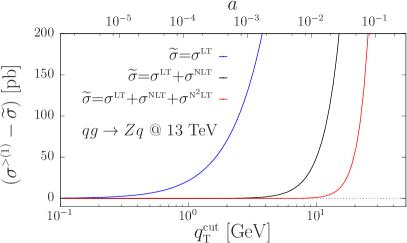
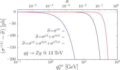
Figure 1: Difference of the total cross sections $\left(\sigma^{\mathchoice{\displaystyle}{\scriptstyle}{\scriptscriptstyle}{\scriptscriptstyle}>(1)}-\widetilde{\sigma}\right)$ as a function of $q_{\mathchoice{\displaystyle}{\scriptstyle}{\scriptscriptstyle}{\scriptscriptstyle}\rm T}^{\mathchoice{\displaystyle}{\scriptstyle}{\scriptscriptstyle}{\scriptscriptstyle}\rm cut}$, for $Z$ boson production, in the $qg\rightarrow Zq$ (left pane) and in the $q\bar{q}\rightarrow Zg$ channel (right pane). The three curves correspond to the three possible choices of $\widetilde{\sigma}$: results for $\widetilde{\sigma}=\sigma^{\mathchoice{\displaystyle}{\scriptstyle}{\scriptscriptstyle}{\scriptscriptstyle}\rm LT}$ are displayed in blue, for $\widetilde{\sigma}=\sigma^{\mathchoice{\displaystyle}{\scriptstyle}{\scriptscriptstyle}{\scriptscriptstyle}\rm LT}+\sigma^{\mathchoice{\displaystyle}{\scriptstyle}{\scriptscriptstyle}{\scriptscriptstyle}\rm NLT}$ are displayed in black and for $\widetilde{\sigma}=\sigma^{\mathchoice{\displaystyle}{\scriptstyle}{\scriptscriptstyle}{\scriptscriptstyle}\rm LT}+\sigma^{\mathchoice{\displaystyle}{\scriptstyle}{\scriptscriptstyle}{\scriptscriptstyle}\rm NLT}+\sigma^{\mathchoice{\displaystyle}{\scriptstyle}{\scriptscriptstyle}{\scriptscriptstyle}\rm N^{2}LT}$ are displayed in red. The corresponding values of $a=\left(q_{\mathchoice{\displaystyle}{\scriptstyle}{\scriptscriptstyle}{\scriptscriptstyle}\rm T}^{\mathchoice{\displaystyle}{\scriptstyle}{\scriptscriptstyle}{\scriptscriptstyle}\rm cut}/m_{\rm\mathchoice{\displaystyle}{\scriptstyle}{\scriptscriptstyle}{\scriptscriptstyle}Z}\right)^{2}$ are displayed on the top of the figure. The statistical errors of the integration are also shown, but they are totally negligible on the scale of the figure.

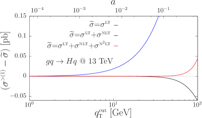
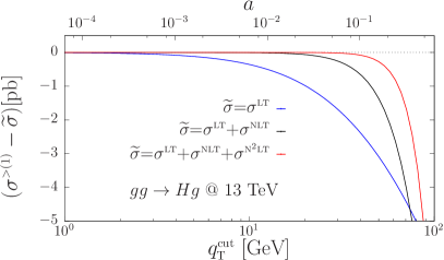
Figure 2: Difference of the total cross sections $\left(\sigma^{\mathchoice{\displaystyle}{\scriptstyle}{\scriptscriptstyle}{\scriptscriptstyle}>(1)}-\widetilde{\sigma}\right)$ as a function of $q_{\mathchoice{\displaystyle}{\scriptstyle}{\scriptscriptstyle}{\scriptscriptstyle}\rm T}^{\mathchoice{\displaystyle}{\scriptstyle}{\scriptscriptstyle}{\scriptscriptstyle}\rm cut}$, for $H$ boson production, in the $qg\rightarrow Hq$ (left pane) and in the $gg\rightarrow Hg$ channel (right pane). Same legend as in fig. 1. The corresponding values of $a=\left(q_{\mathchoice{\displaystyle}{\scriptstyle}{\scriptscriptstyle}{\scriptscriptstyle}\rm T}^{\mathchoice{\displaystyle}{\scriptstyle}{\scriptscriptstyle}{\scriptscriptstyle}\rm cut}/m_{\rm\mathchoice{\displaystyle}{\scriptstyle}{\scriptscriptstyle}{\scriptscriptstyle}H}\right)^{2}$ are displayed on the top of the figure.

We first present our findings separated according to the partonic production channels. In all the figures presented in this paper, the statistical errors of the integration procedure are also displayed, but they are always totally negligible on the scales of the figures.

In fig. 1 we collect the results for the aforementioned cross-section differences, as a function of $q_{\mathchoice{\displaystyle}{\scriptstyle}{\scriptscriptstyle}{\scriptscriptstyle}\rm T}^{\mathchoice{\displaystyle}{\scriptstyle}{\scriptscriptstyle}{\scriptscriptstyle}\rm cut}$, for the $qg\rightarrow Zq$ (left) and $q\bar{q}\rightarrow Zg$ (right) channels, and in fig. 2 we collect similar results for the $gq\rightarrow Hq$ (left) and $gg\rightarrow Hg$ (right) channels. As expected, NLT and N²LT contributions increase the accuracy of the expanded cross section, with respect to the exact one.

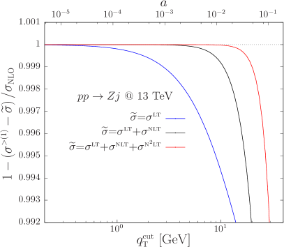
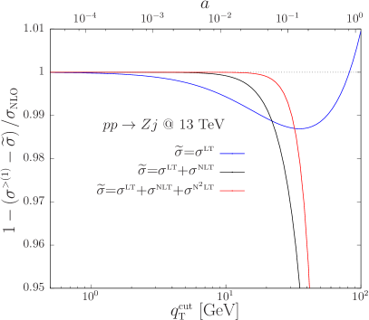
Figure 3: Results for $1-\left(\sigma^{\mathchoice{\displaystyle}{\scriptstyle}{\scriptscriptstyle}{\scriptscriptstyle}>(1)}-\widetilde{\sigma}\right)/\sigma_{\rm\mathchoice{\displaystyle}{\scriptstyle}{\scriptscriptstyle}{\scriptscriptstyle}NLO}$ as a function of $q_{\mathchoice{\displaystyle}{\scriptstyle}{\scriptscriptstyle}{\scriptscriptstyle}\rm T}^{\mathchoice{\displaystyle}{\scriptstyle}{\scriptscriptstyle}{\scriptscriptstyle}\rm cut}$, for $Z$ boson production, in $pp\rightarrow Zj$. Same legend as in fig. 1. In the left pane, the low-$q_{\mathchoice{\displaystyle}{\scriptstyle}{\scriptscriptstyle}{\scriptscriptstyle}\rm T}^{\mathchoice{\displaystyle}{\scriptstyle}{\scriptscriptstyle}{\scriptscriptstyle}\rm cut}$ region is displayed, while, in the right pane, a larger region in $q_{\mathchoice{\displaystyle}{\scriptstyle}{\scriptscriptstyle}{\scriptscriptstyle}\rm T}^{\mathchoice{\displaystyle}{\scriptstyle}{\scriptscriptstyle}{\scriptscriptstyle}\rm cut}$ is shown. The total cross section at NLO for $Z$ production, $\sigma_{\rm\mathchoice{\displaystyle}{\scriptstyle}{\scriptscriptstyle}{\scriptscriptstyle}NLO}$, has been taken equal to 55668.1 pb.

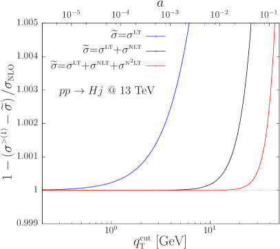
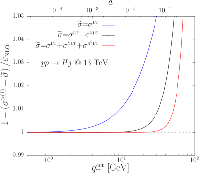
Figure 4: Results for $1-\left(\sigma^{\mathchoice{\displaystyle}{\scriptstyle}{\scriptscriptstyle}{\scriptscriptstyle}>(1)}-\widetilde{\sigma}\right)/\sigma_{\rm\mathchoice{\displaystyle}{\scriptstyle}{\scriptscriptstyle}{\scriptscriptstyle}NLO}$ as a function of $q_{\mathchoice{\displaystyle}{\scriptstyle}{\scriptscriptstyle}{\scriptscriptstyle}\rm T}^{\mathchoice{\displaystyle}{\scriptstyle}{\scriptscriptstyle}{\scriptscriptstyle}\rm cut}$, for $H$ boson production, in $pp\rightarrow Hj$. Same legend as in fig. 1. In the left pane, the low-$q_{\mathchoice{\displaystyle}{\scriptstyle}{\scriptscriptstyle}{\scriptscriptstyle}\rm T}^{\mathchoice{\displaystyle}{\scriptstyle}{\scriptscriptstyle}{\scriptscriptstyle}\rm cut}$ region is displayed, while, in the right pane, a larger region in $q_{\mathchoice{\displaystyle}{\scriptstyle}{\scriptscriptstyle}{\scriptscriptstyle}\rm T}^{\mathchoice{\displaystyle}{\scriptstyle}{\scriptscriptstyle}{\scriptscriptstyle}\rm cut}$ is shown. The total cross section at NLO for $H$ production, $\sigma_{\rm\mathchoice{\displaystyle}{\scriptstyle}{\scriptscriptstyle}{\scriptscriptstyle}NLO}$, has been taken equal to 31.52 pb.

To give a more quantitative estimation of the power-suppressed corrections, we present results for the total hadronic cross section, normalised with respect to the corresponding exact NLO cross section $\sigma_{\rm\mathchoice{\displaystyle}{\scriptstyle}{\scriptscriptstyle}{\scriptscriptstyle}NLO}$ (i.e. including also the virtual contributions). The results are shown in figs. 3 and 4, where we have used $\sigma_{\rm\mathchoice{\displaystyle}{\scriptstyle}{\scriptscriptstyle}{\scriptscriptstyle}NLO}=55668.1$ pb for $Z$ production and 31.52 pb for $H$ production. On the left panes we plot results in a smaller $q_{\mathchoice{\displaystyle}{\scriptstyle}{\scriptscriptstyle}{\scriptscriptstyle}\rm T}^{\mathchoice{\displaystyle}{\scriptstyle}{\scriptscriptstyle}{\scriptscriptstyle}\rm cut}$ region, while, on the right panes, we extend the $q_{\mathchoice{\displaystyle}{\scriptstyle}{\scriptscriptstyle}{\scriptscriptstyle}\rm T}^{\mathchoice{\displaystyle}{\scriptstyle}{\scriptscriptstyle}{\scriptscriptstyle}\rm cut}$ interval to higher values.

These plots show exactly how the residual cutoff dependence of the cross sections changes when the $q_{\mathchoice{\displaystyle}{\scriptstyle}{\scriptscriptstyle}{\scriptscriptstyle}\rm T}$-subtraction counterterm is corrected by the NLT and N²LT power terms. For example, for $Z$ production and for $q_{\mathchoice{\displaystyle}{\scriptstyle}{\scriptscriptstyle}{\scriptscriptstyle}\rm T}^{\mathchoice{\displaystyle}{\scriptstyle}{\scriptscriptstyle}{\scriptscriptstyle}\rm cut}=10$ GeV, corresponding to $a=0.012$, the LT cross section gives an estimate of the exact cross section within the 5‰, that reduces to below the 1‰ when the NLT contribution is added and becomes less than 0.01‰ when also the N²LT is present. For Higgs boson production, the residual cutoff dependence is even more pronounced: in fact, at $q_{\mathchoice{\displaystyle}{\scriptstyle}{\scriptscriptstyle}{\scriptscriptstyle}\rm T}^{\mathchoice{\displaystyle}{\scriptstyle}{\scriptscriptstyle}{\scriptscriptstyle}\rm cut}=10$ GeV, corresponding to $a=0.0064$, the LT is precise within the 1% level. When the NLT is added, the precision reaches the 0.2‰, and is below 0.001‰ with the addition of the N²LT.

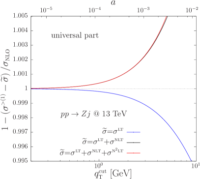
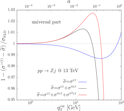
Figure 5: Same as fig. 3, but using only the universal part of $\hat{G}_{ab}^{\mathchoice{\displaystyle}{\scriptstyle}{\scriptscriptstyle}{\scriptscriptstyle}(1,n,m)}(z)$ in computing the cross sections of eqs. (60)–(62).

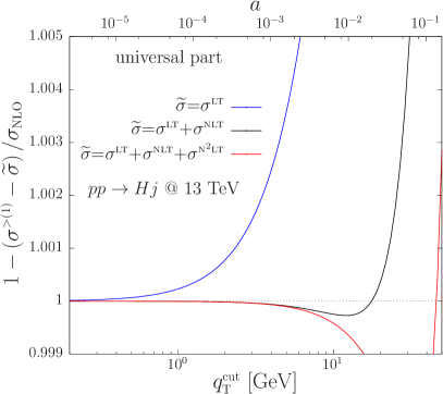
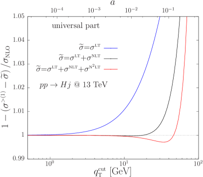
Figure 6: Same as fig. 5 but for Higgs boson production.

An interesting question is to estimate the impact of the universal parts of the $\hat{G}_{ab}^{\mathchoice{\displaystyle}{\scriptstyle}{\scriptscriptstyle}{\scriptscriptstyle}(1,n,m)}(z)$ functions, with respect to the non-universal ones. We have then computed the cross sections in eqs. (60)–(62), taking into account only the universal parts of the $\hat{G}_{ab}^{\mathchoice{\displaystyle}{\scriptstyle}{\scriptscriptstyle}{\scriptscriptstyle}(1,n,m)}(z)$ functions. Our results are displayed in fig. 5, for $Z$ production, and in fig. 6, for $H$ production.

Comparing these figures with the corresponding ones with the full $\hat{G}_{ab}^{\mathchoice{\displaystyle}{\scriptstyle}{\scriptscriptstyle}{\scriptscriptstyle}(1,n,m)}(z)$ functions, i.e. figs. 3 and 4, we see that the non-universal contributions play a crucial role for $Z$ production, while their role is minor in Higgs boson production. This is due to the fact that the non-universal part in eqs. (25) and (• ‣ 3.1) is suppressed by higher powers of $(1-z)$, with respect to the corresponding expression for $Z$ production, in eqs. (23) and (24), confirming the conclusions drawn in sec. 4.2.2.

5 Conclusions

In this paper we considered the production of a colourless system at next-to-leading order in the strong coupling constant $\alpha_{\mathchoice{\displaystyle}{\scriptstyle}{\scriptscriptstyle}{\scriptscriptstyle}\rm S}$. We imposed a transverse-momentum cutoff, $q_{\mathchoice{\displaystyle}{\scriptstyle}{\scriptscriptstyle}{\scriptscriptstyle}\rm T}^{\mathchoice{\displaystyle}{\scriptstyle}{\scriptscriptstyle}{\scriptscriptstyle}\rm cut}$, on the colour-singlet final state and we computed the power corrections for the inclusive cross section in the cutoff, up to the fourth power. Although we studied Drell–Yan vector boson production and Higgs boson production in gluon fusion, the procedure we followed is general and can be applied to other similar cases, up to any order in the powers of $q_{\mathchoice{\displaystyle}{\scriptstyle}{\scriptscriptstyle}{\scriptscriptstyle}\rm T}^{\mathchoice{\displaystyle}{\scriptstyle}{\scriptscriptstyle}{\scriptscriptstyle}\rm cut}$.

We presented analytic results, reproducing the known logarithmic terms from collinear and soft regions of the phase space, along with the finite contribution, and adding new terms as power corrections in $q_{\mathchoice{\displaystyle}{\scriptstyle}{\scriptscriptstyle}{\scriptscriptstyle}\rm T}^{\mathchoice{\displaystyle}{\scriptstyle}{\scriptscriptstyle}{\scriptscriptstyle}\rm cut}$. We found that the logarithmic terms in $q_{\mathchoice{\displaystyle}{\scriptstyle}{\scriptscriptstyle}{\scriptscriptstyle}\rm T}^{\mathchoice{\displaystyle}{\scriptstyle}{\scriptscriptstyle}{\scriptscriptstyle}\rm cut}$ show up at most linearly in the power-correction contributions, consistently with the fact that the LL contribution is a squared logarithm. In addition, no odd-power corrections in $q_{\mathchoice{\displaystyle}{\scriptstyle}{\scriptscriptstyle}{\scriptscriptstyle}\rm T}^{\mathchoice{\displaystyle}{\scriptstyle}{\scriptscriptstyle}{\scriptscriptstyle}\rm cut}$ appeared in our calculation, in agreement with known results in the literature for the NLO differential cross section in colour-singlet production. We do not expect this to be true in general when cuts are applied to the final state.

Along the calculation we kept track of the origin of the newly-computed terms, so that we were able to separate them into a universal part, and a part that depends on the process at stake. In particular we derived and identified the contribution to the universal part coming from soft radiation, present in the diagonal partonic channels for $Z$ and $H$ production. We could also explain some features about the presence of power-suppressed logarithmic terms, appearing in the non-universal part of the power corrections. Furthermore we showed that the knowledge of the squared amplitudes at the next-to-leading-soft approximation is not enough to predict the $(q_{\mathchoice{\displaystyle}{\scriptstyle}{\scriptscriptstyle}{\scriptscriptstyle}\rm T}^{\mathchoice{\displaystyle}{\scriptstyle}{\scriptscriptstyle}{\scriptscriptstyle}\rm cut})^{2}\log q_{\mathchoice{\displaystyle}{\scriptstyle}{\scriptscriptstyle}{\scriptscriptstyle}\rm T}^{\mathchoice{\displaystyle}{\scriptstyle}{\scriptscriptstyle}{\scriptscriptstyle}\rm cut}$ behaviour of the power corrections. The same conclusion can be drawn for the knowledge of the next-to-next-to-leading-soft approximation in predicting the $(q_{\mathchoice{\displaystyle}{\scriptstyle}{\scriptscriptstyle}{\scriptscriptstyle}\rm T}^{\mathchoice{\displaystyle}{\scriptstyle}{\scriptscriptstyle}{\scriptscriptstyle}\rm cut})^{4}\log q_{\mathchoice{\displaystyle}{\scriptstyle}{\scriptscriptstyle}{\scriptscriptstyle}\rm T}^{\mathchoice{\displaystyle}{\scriptstyle}{\scriptscriptstyle}{\scriptscriptstyle}\rm cut}$ power correction.

We also studied the numerical impact of the power terms in the hadronic cross sections for $Z$ and $H$ production at the LHC at 13 TeV, both by keeping track of the different partonic production channels and by summing over all of them. We plotted the behaviours of the cross sections while adding more and more orders of the power-correction terms, as a function of $q_{\mathchoice{\displaystyle}{\scriptstyle}{\scriptscriptstyle}{\scriptscriptstyle}\rm T}^{\mathchoice{\displaystyle}{\scriptstyle}{\scriptscriptstyle}{\scriptscriptstyle}\rm cut}$, and comparing them with the exact cross sections. For example, in $Z$ production and for a value of $q_{\mathchoice{\displaystyle}{\scriptstyle}{\scriptscriptstyle}{\scriptscriptstyle}\rm T}^{\mathchoice{\displaystyle}{\scriptstyle}{\scriptscriptstyle}{\scriptscriptstyle}\rm cut}=10$ GeV, the sensitivity on the cutoff can be reduced from 1‰ to 0.01‰, when adding the $(q_{\mathchoice{\displaystyle}{\scriptstyle}{\scriptscriptstyle}{\scriptscriptstyle}\rm T}^{\mathchoice{\displaystyle}{\scriptstyle}{\scriptscriptstyle}{\scriptscriptstyle}\rm cut})^{4}$ contributions to the $(q_{\mathchoice{\displaystyle}{\scriptstyle}{\scriptscriptstyle}{\scriptscriptstyle}\rm T}^{\mathchoice{\displaystyle}{\scriptstyle}{\scriptscriptstyle}{\scriptscriptstyle}\rm cut})^{2}$ ones. Higgs boson production suffers from a larger sensitivity on the cutoff, and the dependence goes from 1% to 0.2‰, when all the power corrections we computed are added. By performing the same numerical comparisons for just the universal part of the power corrections, we showed that the non-universal contributions play a crucial role for $Z$ production, while their role is minor in Higgs boson production.

The knowledge of the power terms is crucial for understanding both the non-trivial behaviour of cross sections at the boundaries of the phase space, and the resummation structure at subleading orders. Within the $q_{\mathchoice{\displaystyle}{\scriptstyle}{\scriptscriptstyle}{\scriptscriptstyle}\rm T}$-subtraction method, the knowledge of the power terms helps in reducing the cutoff dependence of the cross sections. While the application of the $q_{\mathchoice{\displaystyle}{\scriptstyle}{\scriptscriptstyle}{\scriptscriptstyle}\rm T}$-subtraction method in NLO calculations is superseded by well-known local subtraction methods, at NNLO it still plays a major role, also in view of the fact that, as shown in refs. Grazzini:2017mhc ; Cieri:2018oms , the sensitivity to the numerical value of the cutoff increases at higher orders.

Appendix A Partonic phase space and partonic cross sections at NLO

In this section we collect some basic formulae used to compute the cross section of the partonic process

$$a(p_{1})+b(p_{2})\rightarrow F(q)+c(k)\,,$$ (63)

where $a$, $b$ and $c$ are quarks or gluons, in a combination compatible with the production process of the colourless system $F$. In parentheses, the four momenta of the particles are given.

A.1 Partonic phase space

The standard Mandelstam relativistic invariants are given by

$$s=\left(p_{1}+p_{2}\right)^{2},\quad t=\left(p_{1}-k\right)^{2}=-2p_{1}\cdot k,\quad u=\left(p_{2}-k\right)^{2}=-2p_{2}\cdot k,\quad q^{2}=Q^{2}\,,$$ (64)

and we also define the threshold variable $z$

$$z=\frac{Q^{2}}{s}\,.$$ (65)

The phase-space volume with the appropriate flux factor is given by

$$d\Phi_{2} = \frac{1}{2s}\frac{d^{3}q}{(2\pi)^{3}2q^{0}}\frac{d^{3}k}{(2\pi)^{3}2k^{0}}\,(2\pi)^{4}\delta^{4}\!\left(p_{1}+p_{2}-q-k\right)$$ (66)

$$= \frac{1}{2s}\frac{1}{(2\pi)^{2}}\frac{d^{3}k}{2k^{0}}\,\delta\!\left((p_{1}+p_{2}-k)^{2}-Q^{2}\right).$$

Since the colourless system recoils against the final coloured parton, their transverse momenta are equal. Calling $\theta$ the angle between $p_{1}$ and $k$, we can write

$$q_{\mathchoice{\displaystyle}{\scriptstyle}{\scriptscriptstyle}{\scriptscriptstyle}\rm T} = k_{\mathchoice{\displaystyle}{\scriptstyle}{\scriptscriptstyle}{\scriptscriptstyle}T}=k^{0}\sin\theta\,,$$ (67)

$$t = -\sqrt{s}k^{0}(1-\cos\theta)\,.$$ (68)

Inverting the system, we find the relations

$$k^{0} = -\frac{sq_{\mathchoice{\displaystyle}{\scriptstyle}{\scriptscriptstyle}{\scriptscriptstyle}\rm T}^{2}+t^{2}}{2\sqrt{s}t}\,,$$ (69)

$$\cos\theta = \frac{sq_{\mathchoice{\displaystyle}{\scriptstyle}{\scriptscriptstyle}{\scriptscriptstyle}\rm T}^{2}-t^{2}}{sq_{\mathchoice{\displaystyle}{\scriptstyle}{\scriptscriptstyle}{\scriptscriptstyle}\rm T}^{2}+t^{2}}\,,$$ (70)

which lead to an expression of the phase-space volume in terms of $q_{\mathchoice{\displaystyle}{\scriptstyle}{\scriptscriptstyle}{\scriptscriptstyle}\rm T}$ and $t$

$$\frac{1}{(2\pi)^{2}}\frac{d^{3}k}{2k^{0}}=\frac{1}{4\pi}k^{0}dk^{0}d\cos\theta=-\frac{1}{4\pi}\frac{sq_{\mathchoice{\displaystyle}{\scriptstyle}{\scriptscriptstyle}{\scriptscriptstyle}\rm T}^{2}+t^{2}}{2\sqrt{s}t}\frac{\sqrt{s}}{sq_{\mathchoice{\displaystyle}{\scriptstyle}{\scriptscriptstyle}{\scriptscriptstyle}\rm T}^{2}+t^{2}}dq_{\mathchoice{\displaystyle}{\scriptstyle}{\scriptscriptstyle}{\scriptscriptstyle}\rm T}^{2}\,dt=-\frac{1}{8\pi}\frac{dt}{t}\,dq_{\mathchoice{\displaystyle}{\scriptstyle}{\scriptscriptstyle}{\scriptscriptstyle}\rm T}^{2}\,.$$ (71)

On the other hand, using the identity

$$t\,u=s\,q_{\mathchoice{\displaystyle}{\scriptstyle}{\scriptscriptstyle}{\scriptscriptstyle}\rm T}^{2}\,,$$ (72)

we can write the argument of the $\delta$ function in eq. (66) as

$$(p_{1}+p_{2}-k)^{2}-Q^{2} = s+t+u-Q^{2}=s+t+\frac{sq_{\mathchoice{\displaystyle}{\scriptstyle}{\scriptscriptstyle}{\scriptscriptstyle}\rm T}^{2}}{t}-Q^{2}$$ (73)

$$= \frac{1}{t}\left[t^{2}+\left(s-Q^{2}\right)t+sq_{\mathchoice{\displaystyle}{\scriptstyle}{\scriptscriptstyle}{\scriptscriptstyle}\rm T}^{2}\right]=\frac{1}{t}\left(t-t_{+}\right)\left(t-t_{-}\right),\phantom{aaa}$$

where

$$t_{\pm}=\frac{1}{2}\,\left[Q^{2}-s\pm\sqrt{\left(Q^{2}-s\right)^{2}-4\,s\,q_{\mathchoice{\displaystyle}{\scriptstyle}{\scriptscriptstyle}{\scriptscriptstyle}\rm T}^{2}}\right].$$ (74)

As a consequence, it is possible to write

$$\delta\left(\left(p_{1}+p_{2}-k\right)^{2}-Q^{2}\right)\frac{dt}{t} = \frac{t}{t^{2}-t_{+}t_{-}}\left[\delta\left(t-t_{+}\right)+\delta\left(t-t_{-}\right)\right]dt$$

$$= \frac{1}{\sqrt{\left(Q^{2}-s\right)^{2}-4\,s\,q_{\mathchoice{\displaystyle}{\scriptstyle}{\scriptscriptstyle}{\scriptscriptstyle}\rm T}^{2}}}\left[\delta\left(t-t_{+}\right)+\delta\left(t-t_{-}\right)\right]dt\,,$$

and using eqs. (71) and (A.1), we can write eq. (66) as

$$d\Phi_{2}=\frac{1}{16\pi}\frac{1}{s}\frac{1}{\sqrt{\left(Q^{2}-s\right)^{2}-4\,s\,q_{\mathchoice{\displaystyle}{\scriptstyle}{\scriptscriptstyle}{\scriptscriptstyle}\rm T}^{2}}}\left[\delta\left(t-t_{+}\right)+\delta\left(t-t_{-}\right)\right]dt\,dq_{\mathchoice{\displaystyle}{\scriptstyle}{\scriptscriptstyle}{\scriptscriptstyle}\rm T}^{2}\,.$$ (76)

We then add a dummy integration over the $z$ variable,

$$d\Phi_{2}=\frac{1}{16\pi}\frac{1}{s}\frac{1}{\sqrt{\left(Q^{2}-s\right)^{2}-4\,s\,q_{\mathchoice{\displaystyle}{\scriptstyle}{\scriptscriptstyle}{\scriptscriptstyle}\rm T}^{2}}}\left[\delta\left(t-t_{+}\right)+\delta\left(t-t_{-}\right)\right]\delta\!\left(z-\frac{Q^{2}}{s}\right)dt\,dq_{\mathchoice{\displaystyle}{\scriptstyle}{\scriptscriptstyle}{\scriptscriptstyle}\rm T}^{2}\,dz\,,$$ (77)

that allows us to rewrite the phase-space volume as

$$d\Phi_{2}=\frac{1}{16\pi}\frac{z^{2}}{Q^{4}}\frac{1}{\sqrt{(1-z)^{2}-4z\,{\displaystyle\frac{q_{\mathchoice{\displaystyle}{\scriptstyle}{\scriptscriptstyle}{\scriptscriptstyle}\rm T}^{2}}{Q^{2}}}}}\left[\delta\!\left(t-t_{+}\right)+\delta\!\left(t-t_{-}\right)\right]\delta\!\left(z-\frac{Q^{2}}{s}\right)dt\,dq_{\mathchoice{\displaystyle}{\scriptstyle}{\scriptscriptstyle}{\scriptscriptstyle}\rm T}^{2}\,dz\,,$$ (78)

where

$$t_{\pm}=\frac{Q^{2}}{2z}\,\left[z-1\pm\sqrt{(1-z)^{2}-4z\,{\displaystyle\frac{q_{\mathchoice{\displaystyle}{\scriptstyle}{\scriptscriptstyle}{\scriptscriptstyle}\rm T}^{2}}{Q^{2}}}}\right].$$ (79)

A.2 Partonic cross sections

We can write the partonic cross sections for a $2\rightarrow 2$ process as

$$d\hat{\sigma}=\left|{\cal M}(s,t,u)\right|^{2}d\Phi_{2}\,,$$ (80)

where ${\cal M}$ is the amplitude for the partonic process, that in general can be written as a function of the Mandelstam variables $s$, $t$ and $u$. From eqs. (65) and (72) we can express $s$ and $u$ as functions of $z$, $q_{\mathchoice{\displaystyle}{\scriptstyle}{\scriptscriptstyle}{\scriptscriptstyle}\rm T}$ and $t$, and using eq. (78) we can write

$$d\hat{\sigma} = \frac{1}{16\pi}\frac{z^{2}}{Q^{4}}\frac{1}{\sqrt{(1-z)^{2}-4z\,{\displaystyle\frac{q_{\mathchoice{\displaystyle}{\scriptstyle}{\scriptscriptstyle}{\scriptscriptstyle}\rm T}^{2}}{Q^{2}}}}}\left[\delta\!\left(t-t_{+}\right)+\delta\!\left(t-t_{-}\right)\right]$$ (81)

$$\hskip 113.81102pt{}\times\delta\!\left(z-\frac{Q^{2}}{s}\right)\left|{\cal M}\left(z,t,q_{\mathchoice{\displaystyle}{\scriptstyle}{\scriptscriptstyle}{\scriptscriptstyle}\rm T}\right)\right|^{2}dt\,dq_{\mathchoice{\displaystyle}{\scriptstyle}{\scriptscriptstyle}{\scriptscriptstyle}\rm T}^{2}\,dz$$

$$= \frac{1}{16\pi}\frac{z^{2}}{Q^{4}\,dz}\frac{1}{\sqrt{(1-z)^{2}-4z\,{\displaystyle\frac{q_{\mathchoice{\displaystyle}{\scriptstyle}{\scriptscriptstyle}{\scriptscriptstyle}\rm T}^{2}}{Q^{2}}}}}\left[\left|{\cal M}\left(z,t_{+},q_{\mathchoice{\displaystyle}{\scriptstyle}{\scriptscriptstyle}{\scriptscriptstyle}\rm T}\right)\right|^{2}+\left|{\cal M}\left(z,t_{-},q_{\mathchoice{\displaystyle}{\scriptstyle}{\scriptscriptstyle}{\scriptscriptstyle}\rm T}\right)\right|^{2}\right]$$

$$\hskip 113.81102pt{}\times\delta\!\left(\!z-\frac{Q^{2}}{s}\right)dq_{\mathchoice{\displaystyle}{\scriptstyle}{\scriptscriptstyle}{\scriptscriptstyle}\rm T}^{2}\,dz$$

$$= \frac{d\hat{\sigma}_{ab}\!\left(q_{\mathchoice{\displaystyle}{\scriptstyle}{\scriptscriptstyle}{\scriptscriptstyle}\rm T},z\right)}{dq_{\mathchoice{\displaystyle}{\scriptstyle}{\scriptscriptstyle}{\scriptscriptstyle}\rm T}^{2}}\,\delta\!\left(\!z-\frac{Q^{2}}{s}\right)dq_{\mathchoice{\displaystyle}{\scriptstyle}{\scriptscriptstyle}{\scriptscriptstyle}\rm T}^{2}\,dz\,,$$

where we have defined

$$\frac{d\hat{\sigma}_{ab}\!\left(q_{\mathchoice{\displaystyle}{\scriptstyle}{\scriptscriptstyle}{\scriptscriptstyle}\rm T},z\right)}{dq_{\mathchoice{\displaystyle}{\scriptstyle}{\scriptscriptstyle}{\scriptscriptstyle}\rm T}^{2}}\equiv\frac{1}{16\pi}\frac{z^{2}}{Q^{4}}\frac{1}{\sqrt{(1-z)^{2}-4z\,{\displaystyle\frac{q_{\mathchoice{\displaystyle}{\scriptstyle}{\scriptscriptstyle}{\scriptscriptstyle}\rm T}^{2}}{Q^{2}}}}}\left[\left|{\cal M}\left(z,t_{+},q_{\mathchoice{\displaystyle}{\scriptstyle}{\scriptscriptstyle}{\scriptscriptstyle}\rm T}\right)\right|^{2}+\left|{\cal M}\left(z,t_{-},q_{\mathchoice{\displaystyle}{\scriptstyle}{\scriptscriptstyle}{\scriptscriptstyle}\rm T}\right)\right|^{2}\right].$$ (82)

A.3 Squared amplitudes and their soft limit

In this section, for completeness, we collect the squared amplitudes $\left|{\cal M}(s,t,u)\right|^{2}$ for $V$+jet and $H$+jet, at the lowest order in $\alpha_{\mathchoice{\displaystyle}{\scriptstyle}{\scriptscriptstyle}{\scriptscriptstyle}\rm S}$, stripped off of trivial coupling, colour and spin factors. The normalization of the following amplitudes is such that

$$\frac{z}{2}\,\frac{q_{\mathchoice{\displaystyle}{\scriptstyle}{\scriptscriptstyle}{\scriptscriptstyle}\rm T}^{2}}{Q^{2}}\left[\left|{\cal M}\left(z,t_{+},q_{\mathchoice{\displaystyle}{\scriptstyle}{\scriptscriptstyle}{\scriptscriptstyle}\rm T}\right)\right|^{2}+\left|{\cal M}\left(z,t_{-},q_{\mathchoice{\displaystyle}{\scriptstyle}{\scriptscriptstyle}{\scriptscriptstyle}\rm T}\right)\right|^{2}\right]$$ (83)

is exactly the numerator of eqs. (10)–(14).

Together with the exact squared matrix elements, we give also the soft behaviour of the amplitudes, using the energy $k^{0}$ of the final-state parton as expansion parameter. We have computed the soft expansion adopting the following procedure: we first got rid of $s$ in favour of $Q^{2}$, $t$ and $u$ using the identity

$$s=Q^{2}-t-u\,.$$ (84)

In this way, the only dependence on the energy of the final-state parton is through $t$ and $u$, that are linearly dependent on $k^{0}$ (see eq. (64)). Then we perform a Laurent expansion in $k^{0}$, and define leading soft (LS) the term proportional to the highest negative power of $k^{0}$, next-to-leading soft (N¹LS) the subsequent term, and so on. Finally we re-express all the soft-expansion contributions in terms of $t$ and $u$. As a result, at each order of the expansion, all the terms proportional to a given power of $k^{0}$ are included, and only them. This is an unambiguous way to define the softness order of the expansion.

$\boldsymbol{V}$ production

• $q(\bar{q})+g\rightarrow V+q(\bar{q})$

  The exact squared amplitude is given by

  $$\left|{\cal M}(s,t,u)\right|^{2}=-2\left[\frac{t}{s}+\frac{s}{t}+2\,\frac{Q^{2}u}{st}\right]$$ (85)

  with soft-expansion terms

  $$\left|{\cal M}\right|^{2}_{\rm\mathchoice{\displaystyle}{\scriptstyle}{\scriptscriptstyle}{\scriptscriptstyle}LS} = -2\,\frac{Q^{2}}{t}$$ (86)

  $$\left|{\cal M}\right|^{2}_{\rm\mathchoice{\displaystyle}{\scriptstyle}{\scriptscriptstyle}{\scriptscriptstyle}N^{1}LS} = -2\,\frac{u}{t}+2\$$ (87)

  $$\left|{\cal M}\right|^{2}_{\rm\mathchoice{\displaystyle}{\scriptstyle}{\scriptscriptstyle}{\scriptscriptstyle}N^{2}LS} = -\frac{2}{Q^{2}}\left[2\frac{u^{2}}{t}+2u+t\right]$$ (88)

  $$\left|{\cal M}\right|^{2}_{\rm\mathchoice{\displaystyle}{\scriptstyle}{\scriptscriptstyle}{\scriptscriptstyle}N^{3}LS} = -\frac{2}{Q^{4}}\left[2\,{\frac{u^{3}}{t}}+4\,u^{2}+3\,tu+t^{2}\right]$$ (89)

  $$\left|{\cal M}\right|^{2}_{\rm\mathchoice{\displaystyle}{\scriptstyle}{\scriptscriptstyle}{\scriptscriptstyle}N^{4}LS} = \ldots$$ (90)

• $q+\bar{q}\rightarrow V+g$

  The exact squared amplitude is given by

  $$\left|{\cal M}(s,t,u)\right|^{2}=\frac{4\,Q^{4}}{tu}-4\left[\frac{Q^{2}}{u}+\frac{Q^{2}}{t}\right]+2\left[\frac{u}{t}+\frac{t}{u}\right]$$ (91)

  with soft-expansion terms

  $$\left|{\cal M}\right|^{2}_{\rm\mathchoice{\displaystyle}{\scriptstyle}{\scriptscriptstyle}{\scriptscriptstyle}LS} = 4\,\frac{Q^{4}}{t\,u}$$ (92)

  $$\left|{\cal M}\right|^{2}_{\rm\mathchoice{\displaystyle}{\scriptstyle}{\scriptscriptstyle}{\scriptscriptstyle}N^{1}LS} = -4\left[\frac{Q^{2}}{t}+\frac{Q^{2}}{u}\right]$$ (93)

  $$\left|{\cal M}\right|^{2}_{\rm\mathchoice{\displaystyle}{\scriptstyle}{\scriptscriptstyle}{\scriptscriptstyle}N^{2}LS} = 2\left[\frac{u}{t}+\frac{t}{u}\right]$$ (94)

  $$\left|{\cal M}\right|^{2}_{\rm\mathchoice{\displaystyle}{\scriptstyle}{\scriptscriptstyle}{\scriptscriptstyle}N^{{\it n}}LS} = 0\,,\qquad\qquad n\geq 3$$ (95)

We notice that, for $q(\bar{q})+g\rightarrow V+q(\bar{q})$ production, the LS term of eq. (86) has only one negative power of $k^{0}$, while in $q+\bar{q}\rightarrow V+g$ the LS term of eq. (92) has two negative powers of $k^{0}$, in agreement with the eikonal approximation for soft-gluon emission.

$\boldsymbol{H}$ production

• $g+q(\bar{q})\rightarrow H+q(\bar{q})$

  The exact squared amplitude is given by

  $$\left|{\cal M}(s,t,u)\right|^{2}=-\frac{2}{Q^{2}}\frac{s^{2}+u^{2}}{t}$$ (96)

  with soft-expansion terms

  $$\left|{\cal M}\right|^{2}_{\rm\mathchoice{\displaystyle}{\scriptstyle}{\scriptscriptstyle}{\scriptscriptstyle}LS} = -2\frac{Q^{2}}{t}$$ (97)

  $$\left|{\cal M}\right|^{2}_{\rm\mathchoice{\displaystyle}{\scriptstyle}{\scriptscriptstyle}{\scriptscriptstyle}N^{1}LS} = 4\frac{u}{t}+4$$ (98)

  $$\left|{\cal M}\right|^{2}_{\rm\mathchoice{\displaystyle}{\scriptstyle}{\scriptscriptstyle}{\scriptscriptstyle}N^{2}LS} = -\frac{2}{Q^{2}}\left[2\frac{u^{2}}{t}+2\,u+t\right]$$ (99)

  $$\left|{\cal M}\right|^{2}_{\rm\mathchoice{\displaystyle}{\scriptstyle}{\scriptscriptstyle}{\scriptscriptstyle}N^{{\it n}}LS} = 0\,,\qquad\qquad n\geq 3$$ (100)

• $g+g\rightarrow H+g$

  The exact squared amplitude is given by

  $$\left|{\cal M}(s,t,u)\right|^{2}=\frac{2}{Q^{2}}\frac{\left(Q^{2}\right)^{4}+s^{4}+t^{4}+u^{4}}{s\,t\,u}$$ (101)

  with soft-expansion terms

  $$\left|{\cal M}\right|^{2}_{\rm\mathchoice{\displaystyle}{\scriptstyle}{\scriptscriptstyle}{\scriptscriptstyle}LS} = 4\,\frac{Q^{4}}{t\,u}$$ (102)

  $$\left|{\cal M}\right|^{2}_{\rm\mathchoice{\displaystyle}{\scriptstyle}{\scriptscriptstyle}{\scriptscriptstyle}N^{1}LS} = -4\left[\frac{Q^{2}}{t}+\frac{Q^{2}}{u}\right]$$ (103)

  $$\left|{\cal M}\right|^{2}_{\rm\mathchoice{\displaystyle}{\scriptstyle}{\scriptscriptstyle}{\scriptscriptstyle}N^{2}LS} = 8\left[\frac{u}{t}+\frac{t}{u}+2\right]$$ (104)

  $$\left|{\cal M}\right|^{2}_{\rm\mathchoice{\displaystyle}{\scriptstyle}{\scriptscriptstyle}{\scriptscriptstyle}N^{3}LS} = 0$$ (105)

  $$\left|{\cal M}\right|^{2}_{\rm\mathchoice{\displaystyle}{\scriptstyle}{\scriptscriptstyle}{\scriptscriptstyle}N^{4}LS} = \frac{4}{Q^{4}}\frac{\left(u^{2}+t\,u+t^{2}\right)^{2}}{t\,u}$$ (106)

  $$\left|{\cal M}\right|^{2}_{\rm\mathchoice{\displaystyle}{\scriptstyle}{\scriptscriptstyle}{\scriptscriptstyle}N^{5}LS} = \ldots$$ (107)

Similar conclusions to $V$ production can be drawn for $H$ production: one negative power of $k^{0}$ in $g+q(\bar{q})\rightarrow H+q(\bar{q})$, see eq. (97), and two negative powers for $g+g\rightarrow H+g$, see eq. (102).

Appendix B Process-independent procedure for extending the $\boldsymbol{z}$ integration

In this section we describe the procedure followed to extend the integration range of the $z$ variable up to 1, as displayed in eq. (34), performing an expansion in $a$. We consider an integral of the following form

$$I=\int_{\tau}^{1-f(a)}dz\,l(z)\,g(z)\,,$$ (108)

with $g(z)$ not defined for $z>1-f(a)$, $l(z)$ well behaved for $\tau\leq z\leq 1$ and $l(z)=0$ for $z<\tau$. We also assume that $l(z)$ is ${\cal C}^{\infty}$, so that we can derive it as many times as necessary. We then suppose that $g(z)$ can be written as an expansion in (negative) powers of $(1-z)$

$$g(z)=g_{0}(z,a)+\frac{g_{1}(z,a)}{1-z}+\frac{g_{2}(z,a)}{(1-z)^{2}}+\ldots=\sum_{n=0}^{\infty}\frac{g_{n}(z,a)}{(1-z)^{n}}\,,$$ (109)

where, in $z=1$, the $g_{i}(z,a)$ are not singular or have an integrable singularity. If not identically zero everywhere, the $g_{i}(z,a)$ are different from 0 for $z=1$ and $i\geq 1$, and, in general, the $g_{i}(z,a)$ functions contain growing powers of $a$ as $i$ increases.

The point we would like to make here is that the right-hand side of eq. (109) is convergent only for $z\leq 1-f(a)$, and it converges to $g(z)$. For $z>1-f(a)$ the series does not converge to $g(z)$, otherwise $g(z)$ would be defined in this region too.

We also assume that we can exchange the order of integration and summation of the series, and we write eq. (108) as

$$I=\sum_{n=0}^{\infty}I_{n}\,,$$ (110)

where

$$I_{n}\equiv\int_{\tau}^{1-f(a)}dz\,l(z)\,\frac{g_{n}(z,a)}{(1-z)^{n}}=\int_{0}^{1-f(a)}dz\,l(z)\,\frac{g_{n}(z,a)}{(1-z)^{n}}\,,$$ (111)

where we have extended the $z$-integration down to 0, since $l(z)=0$ for $z<\tau$. Each term of the series can now be manipulated as shown in the following.

$\boldsymbol{I_{0}}$

$$I_{0} = \int_{0}^{1-f(a)}dz\,l(z)\,g_{0}(z,a)=\int_{0}^{1}dz\,l(z)\,g_{0}(z,a)-\int_{1-f(a)}^{1}dz\,l(z)\,g_{0}(z,a)$$ (112)

is finite and poses no problems.

$\boldsymbol{I_{1}}$

$$I_{1} = {}+\int_{0}^{1-f(a)}dz\big{[}l(z)-l(1)\big{]}\frac{g_{1}(z,a)}{1-z}+\int_{0}^{1-f(a)}dz\,l(1)\,\frac{g_{1}(z,a)}{1-z}$$ (113)

$$= {}+\int_{0}^{1}dz\big{[}l(z)-l(1)\big{]}\frac{g_{1}(z,a)}{1-z}-\int_{1-f(a)}^{1}dz\big{[}l(z)-l(1)\big{]}\frac{g_{1}(z,a)}{1-z}$$

$${}+\int_{0}^{1-f(a)}dz\,l(1)\,\frac{g_{1}(z,a)}{1-z}\,,$$

where we have added and subtracted the first term of the Taylor expansion of $l(z)$ around the point $z=1$, and performed straightforward manipulations of the integration limits. The first and second integrands in the above equation are well behaved when $z\rightarrow 1$, since the numerator goes to zero at least as fast as $(1-z)$, cancelling the divergence of the denominator.

$\boldsymbol{I_{2}}$

In a similar way, we can manipulate $I_{2}$ to have

$$I_{2} = {}+\int_{0}^{1}dz\big{[}l(z)-l(1)-(z-1)\,l^{(1)}(1)\big{]}\frac{g_{2}(z,a)}{(1-z)^{2}}$$ (114)

$${}-\int_{1-f(a)}^{1}dz\big{[}l(z)-l(1)-l^{(1)}(1)\,(z-1)\big{]}\frac{g_{2}(z,a)}{(1-z)^{2}}$$

$${}+\int_{0}^{1-f(a)}dz\big{[}l(1)+l^{(1)}(1)\,(z-1)\big{]}\frac{g_{2}(z,a)}{(1-z)^{2}}\,,$$

where we have added and subtracted the first two terms of the Taylor expansion of $l(z)$ around $z=1$. Again the first two integrands are finite when $z\rightarrow 1$, since the numerator is $\mathcal{O}\!\left((1-z)^{2}\right)$.

Final expression

The same procedure can be applied to all the integrals $I_{n}$ and leads to the final result

$$I=\tilde{I}_{1}+\tilde{I}_{2}+\tilde{I}_{3}\,,$$ (115)

where

$$\tilde{I}_{1} = {}+\int_{0}^{1}dz\,l(z)\,g_{0}(z,a)$$ (116)

$${}+\int_{0}^{1}dz\left[l(z)-l(1)\right]\frac{g_{1}(z,a)}{1-z}$$

$${}+\int_{0}^{1}dz\left[l(z)-l(1)-l^{(1)}(1)\,(z-1)\right]\frac{g_{2}(z,a)}{(1-z)^{2}}+\ldots$$

$$\tilde{I}_{2} = {}+\int_{0}^{1-f(a)}dz\,l(1)\big{[}g(z)-g_{0}(z,a)\big{]}$$ (117)

$${}+\int_{0}^{1-f(a)}dz\,l^{(1)}(1)\,(z-1)\left[g(z)-g_{0}(z,a)-\frac{g_{1}(z,a)}{1-z}\right]$$

$${}+\int_{0}^{1-f(a)}dz\,\frac{1}{2!}\,l^{(2)}(1)\,(z-1)^{2}\left[g(z)-g_{0}(z,a)-\frac{g_{1}(z,a)}{1-z}-\frac{g_{2}(z,a)}{(1-z)^{2}}\right]+\ldots\phantom{aaaa}$$

$$\tilde{I}_{3} = {}-\int_{1-f(a)}^{1}dz\,l(z)\,g_{0}(z,a)$$ (118)

$${}-\int_{1-f(a)}^{1}dz\big{[}l(z)-l(1)\big{]}\frac{g_{1}(z,a)}{1-z}$$

$${}-\int_{1-f(a)}^{1}dz\left[l(z)-l(1)-l^{(1)}(1)\,(z-1)\right]\frac{g_{2}(z,a)}{(1-z)^{2}}+\ldots$$

Notice that in $\tilde{I}_{2}$ the sum of the terms of the series add up to give back $g(z)$, since the upper integration limit is $1-f(a)$, so that we are within the region of convergence of the series. The integrals in $\tilde{I}_{2}$ have to be evaluated exactly analytically, and this is the harsh part of the calculation.

The integrals in $\tilde{I}_{3}$ can instead be computed by performing an expansion in $a$, and this part of the calculation poses no problems. Examples of resolution of these integrals are given in appendix C.

Finally, by using of the plus distributions defined in appendix E, we can write $\tilde{I}_{1}$ in a more compact form

$$\tilde{I}_{1}=\!\int_{0}^{1}dz\,l(z)\,g_{0}(z,a)+\int_{0}^{1}dz\,l(z)\!\left[\frac{g_{1}(z,a)}{1-z}\right]_{+}+\int_{0}^{1}dz\,l(z)\!\left[\frac{g_{2}(z,a)}{(1-z)^{2}}\right]_{2+}+\ldots\phantom{aaa}$$ (119)

This completes our process-independent procedure for the manipulation of the integral in eq. (108).

Appendix C Detailed derivation of the results for $\boldsymbol{V}$ and $\boldsymbol{H}$ production

In this section we present in detail how we applied the method described in appendix B to perform the series expansion in $a$ for every production channel of the processes at stake. In particular, we specify for each channel which functions are assumed to be the $l(z)$ and $g(z)$ functions of eq. (108).

For ease of notation, in the following sections, the subscripts of the parton luminosities are suppressed, since any misunderstanding is prevented by the title of the section itself.

Also, in the summary of each of the following sections, a distinction is made while separating the final result in a universal and a non-universal part. As detailed in secs. 2.2 and 3.1, the contributions proportional to the Altarelli–Parisi splitting functions constitute what we call the universal part of the results. The remaining ones constitute the non-universal one.

C.1 $\boldsymbol{V}$ production: $\boldsymbol{qg}$ channel

The relevant integral, corresponding to that in eq. (108), is

$$I = \int_{\tau}^{1-f(a)}dz\,{\cal L}\left(\frac{\tau}{z}\right)\left\{\frac{1}{2z}\,(1+3z)(1-z)\,\sqrt{1-\frac{4az}{(1-z)^{2}}}\right.$$ (120)

$$\left.{}+p_{qg}(z)\frac{1}{z}\left[-\log\frac{az}{(1-z)^{2}}+2\log\frac{1}{2}\left(\sqrt{1-\frac{4az}{(1-z)^{2}}}+1\right)\right]\right\},\phantom{aaaaa}$$

where

$$p_{qg}(z)=2z^{2}-2z+1\,.$$ (121)

We can express $I$ as the sum of three integrals

$$I=I^{a}+I^{b}+I^{c}\,,$$ (122)

where

$$I^{a} = \int_{\tau}^{1-f(a)}dz\,\frac{1}{2z}\,(1+3z)(1-z)\,{\cal L}\left(\frac{\tau}{z}\right)\sqrt{1-\frac{4az}{(1-z)^{2}}}\,,$$ (123)

$$I^{b} = -\int_{\tau}^{1-f(a)}dz\,p_{qg}(z)\,\frac{1}{z}\,{\cal L}\left(\frac{\tau}{z}\right)\log\frac{az}{(1-z)^{2}}\,,$$ (124)

$$I^{c} = \int_{\tau}^{1-f(a)}dz\,p_{qg}(z)\,\frac{2}{z}\,{\cal L}\left(\frac{\tau}{z}\right)\log\frac{1}{2}\left(\sqrt{1-\frac{4az}{(1-z)^{2}}}+1\right),$$ (125)

and for each of the three integrals we apply the procedure detailed in appendix B.

Integral $\boldsymbol{I^{a}}$

We define

$$l(z) = \frac{1}{2z}\,(1+3z)\,{\cal L}\left(\frac{\tau}{z}\right),$$ (126)

$$g(z) = (1-z)\,\sqrt{1-\frac{4az}{(1-z)^{2}}}\,,$$ (127)

and expanding $g(z)$ according to eq. (109), we have

$$g(z) = (1-z)-\frac{2az}{1-z}-\frac{2a^{2}z^{2}}{(1-z)^{3}}+\mathcal{O}\!\left(a^{3}\right)$$ (128)

so that

$$g_{0}(z,a)=1-z\,,\qquad g_{1}(z,a)=-2az\,,\qquad g_{2}(z,a)=0\,,\qquad g_{3}(z,a)=-2a^{2}z^{2}\,.$$ (129)

With this assignment of the different terms of the expansion of $g(z)$, we perform the integrations in eqs. (116)–(118).

Integral $\boldsymbol{I^{b}}$

The integrand of $I^{b}$ is defined up to $z=1$. For this reason, the computation of this contribution is easier than the previous one. In particular we can write

$$I^{b}\equiv I^{b}_{1}+I^{b}_{2}\,,$$ (130)

where

$$I^{b}_{1} = -\int_{0}^{1}dz\,p_{qg}(z)\,\frac{1}{z}\log\frac{az}{(1-z)^{2}}\,{\cal L}\left(\frac{\tau}{z}\right),$$ (131)

$$I^{b}_{2} = +\int_{1-f(a)}^{1}dz\,p_{qg}(z)\,\frac{1}{z}\log\frac{az}{(1-z)^{2}}\,{\cal L}\left(\frac{\tau}{z}\right).$$ (132)

Defining

$$l(z)=\left(2z^{2}-2z+1\right)\frac{1}{z}\,{\cal L}\left(\frac{\tau}{z}\right),$$ (133)

we expand it as a power series in $(z-1)$, so that

$$I^{b}_{2}=\sum_{n=0}^{\infty}\frac{1}{n!}\,l^{(n)}(1)\int_{1-f(a)}^{1}dz\,(z-1)^{n}\log\frac{az}{(1-z)^{2}}$$ (134)

and the integration becomes straightforward.

Integral $\boldsymbol{I^{c}}$

We define

$$l(z) = \frac{2}{z}\left(2z^{2}-2z+1\right)\,{\cal L}\left(\frac{\tau}{z}\right),$$ (135)

$$g(z) = \log\frac{1}{2}\left(\sqrt{1-\frac{4az}{(1-z)^{2}}}+1\right),$$ (136)

and expanding $g(z)$ according to eq. (109), we have

$$g(z)=-\frac{az}{(1-z)^{2}}-\frac{3}{2}\frac{a^{2}z^{2}}{(1-z)^{4}}+\mathcal{O}\!\left(a^{3}\right),$$ (137)

so that

$$g_{0}(z,a)=g_{1}(z,a)=g_{3}(z,a)=0\,,\qquad g_{2}(z,a)=-az\,,\qquad g_{4}(z,a)=-\frac{3}{2}a^{2}z^{2}\,.$$ (138)

We then perform the integrations in eqs. (116)–(118).

C.1.1 Summary

Summarising our results, and writing $I$ in eq. (120) as a sum of the universal and the non-universal part, we have

$$I=I^{\mathchoice{\displaystyle}{\scriptstyle}{\scriptscriptstyle}{\scriptscriptstyle}\rm U}+I^{\mathchoice{\displaystyle}{\scriptstyle}{\scriptscriptstyle}{\scriptscriptstyle}\rm R}\,,$$ (139)

where

$$I^{\mathchoice{\displaystyle}{\scriptstyle}{\scriptscriptstyle}{\scriptscriptstyle}\rm U} = {}-\log(a)\int_{0}^{1}dz\,\frac{1}{z}\,p_{qg}(z)\,{\cal L}\left(\frac{\tau}{z}\right)-\int_{0}^{1}dz\,\frac{1}{z}\,p_{qg}(z)\,\log\frac{z}{(1-z)^{2}}\,{\cal L}\left(\frac{\tau}{z}\right)$$ (140)

$${}-2\,a\int_{0}^{1}dz\,p_{qg}(z)\,{\cal L}\left(\frac{\tau}{z}\right)\left[\frac{1}{(1-z)^{2}}\right]_{2+}-3\,a^{2}\!\int_{0}^{1}\!dz\,z\,p_{qg}(z)\,{\cal L}\left(\frac{\tau}{z}\right)\!\left[\frac{1}{(1-z)^{4}}\right]_{4+}$$

$${}+\left\{-2\,{\cal L}(\tau)+\,\tau\,{\cal L}^{(1)}(\tau)\right\}a\log(a)+{\cal L}(\tau)\,a$$

$${}+\left\{-3\,{\cal L}(\tau)+3\,\tau\,{\cal L}^{(1)}(\tau)-\frac{3}{4}\,\tau^{2}\,{\cal L}^{(2)}(\tau)+\frac{1}{4}\,\tau^{3}\,{\cal L}^{(3)}(\tau)\right\}a^{2}\log(a)$$

$${}+\left\{\frac{9}{4}\,{\cal L}(\tau)-\frac{1}{4}\,\tau\,{\cal L}^{(1)}(\tau)+\frac{1}{4}\,\tau^{2}\,{\cal L}^{(2)}(\tau)+\frac{1}{6}\,\tau^{3}\,{\cal L}^{(3)}(\tau)\right\}a^{2}+\mathcal{O}\!\left(a^{\frac{5}{2}}\log(a)\right),\phantom{aaaa}$$

$$I^{\mathchoice{\displaystyle}{\scriptstyle}{\scriptscriptstyle}{\scriptscriptstyle}\rm R} = {}+\int_{0}^{1}dz\,\frac{1}{2z}\,(1+3z)(1-z)\,{\cal L}\left(\frac{\tau}{z}\right)-a\int_{0}^{1}dz\,(1+3z)\,{\cal L}\left(\frac{\tau}{z}\right)\left[\frac{1}{1-z}\right]_{+}$$ (141)

$${}-a^{2}\int_{0}^{1}\!dz\,z\,(1+3z)\,{\cal L}\left(\frac{\tau}{z}\right)\!\left[\frac{1}{(1-z)^{3}}\right]_{3+}$$

$${}+2\,{\cal L}(\tau)\,a\log(a)-2\,{\cal L}(\tau)\,a$$

$${}+\left\{\frac{3}{2}\,{\cal L}(\tau)-\frac{3}{2}\,\tau\,{\cal L}^{(1)}(\tau)+\tau^{2}\,{\cal L}^{(2)}(\tau)\right\}a^{2}\log(a)$$

$${}+\left\{-\frac{7}{4}\,{\cal L}(\tau)+\frac{5}{4}\,\tau\,{\cal L}^{(1)}(\tau)+\frac{1}{2}\,\tau^{2}\,{\cal L}^{(2)}(\tau)\right\}a^{2}+\mathcal{O}\!\left(a^{\frac{5}{2}}\log(a)\right).$$

Then, writing $I^{\mathchoice{\displaystyle}{\scriptstyle}{\scriptscriptstyle}{\scriptscriptstyle}\rm U}$ and $I^{\mathchoice{\displaystyle}{\scriptstyle}{\scriptscriptstyle}{\scriptscriptstyle}\rm R}$ in the form

$$I^{\mathchoice{\displaystyle}{\scriptstyle}{\scriptscriptstyle}{\scriptscriptstyle}\rm U}=\int_{0}^{1}\frac{dz}{z}\,{\cal L}\left(\frac{\tau}{z}\right)\hat{g}^{\mathchoice{\displaystyle}{\scriptstyle}{\scriptscriptstyle}{\scriptscriptstyle}\rm U(1)}_{qg}(z)\,,\qquad\qquad I^{\mathchoice{\displaystyle}{\scriptstyle}{\scriptscriptstyle}{\scriptscriptstyle}\rm R}=\int_{0}^{1}\frac{dz}{z}\,{\cal L}\left(\frac{\tau}{z}\right)\hat{g}^{\mathchoice{\displaystyle}{\scriptstyle}{\scriptscriptstyle}{\scriptscriptstyle}\rm R(1)}_{qg}(z)\,,$$ (142)

we get the expression of $\hat{g}^{\mathchoice{\displaystyle}{\scriptstyle}{\scriptscriptstyle}{\scriptscriptstyle}\rm U(1)}_{qg}(z)$ and $\hat{g}^{\mathchoice{\displaystyle}{\scriptstyle}{\scriptscriptstyle}{\scriptscriptstyle}\rm R(1)}_{qg}(z)$ in eqs. (37) and (38), respectively.

C.2 $\boldsymbol{V}$ production: $\boldsymbol{q\bar{q}}$ channel

The relevant integral, corresponding to that in eq. (108), is

$$I = \int_{\tau}^{1-f(a)}dz\,{\cal L}\left(\frac{\tau}{z}\right)\left\{-\frac{2}{z}\,(1-z)\,\sqrt{1-\frac{4az}{(1-z)^{2}}}\right.$$ (143)

$$\left.+\,\frac{2}{z}\,\hat{p}_{qq}(z)\left[-\log\frac{az}{(1-z)^{2}}+2\log\frac{1}{2}\left(\sqrt{1-\frac{4az}{(1-z)^{2}}}+1\right)\right]\right\},\phantom{aa}$$

where

$$\hat{p}_{qq}(z)=\frac{1+z^{2}}{1-z}\,.$$ (144)

We can express $I$ as the sum of three integrals

$$I=I^{a}+I^{b}+I^{c}\,,$$ (145)

where

$$I^{a} = -\int_{\tau}^{1-f(a)}dz\,{\cal L}\left(\frac{\tau}{z}\right)\frac{2}{z}(1-z)\,\sqrt{1-\frac{4az}{(1-z)^{2}}}\,,$$ (146)

$$I^{b} = -\int_{\tau}^{1-f(a)}dz\,\frac{2}{z}\,\hat{p}_{qq}(z)\,{\cal L}\left(\frac{\tau}{z}\right)\log\frac{az}{(1-z)^{2}}\,,$$ (147)

$$I^{c} = \int_{\tau}^{1-f(a)}dz\,\frac{4}{z}\,\hat{p}_{qq}(z)\,{\cal L}\left(\frac{\tau}{z}\right)\log\frac{1}{2}\left(\sqrt{1-\frac{4az}{(1-z)^{2}}}+1\right),$$ (148)

and for each of the three integrals we apply the procedure detailed in appendix B.

Integral $\boldsymbol{I^{a}}$

We define

$$l(z) = -\frac{2}{z}\,{\cal L}\left(\frac{\tau}{z}\right),$$ (149)

$$g(z) = (1-z)\,\sqrt{1-\frac{4az}{(1-z)^{2}}}\,,$$ (150)

and expanding $g(z)$ according to eq. (109), we have

$$g(z) = (1-z)-\frac{2az}{1-z}-\frac{2a^{2}z^{2}}{(1-z)^{3}}+\mathcal{O}\!\left(a^{3}\right),$$ (151)

so that

$$g_{0}(z,a)=1-z\,,\qquad g_{1}(z,a)=-2az\,,\qquad g_{2}(z,a)=0\,,\qquad g_{3}(z,a)=-2a^{2}z^{2}\,.$$ (152)

We then perform the integrations in eqs. (116)–(118).

Integral $\boldsymbol{I^{b}}$

We start by separating $I^{b}$ into two further integrals, writing

$$I^{b}=I^{b1}+I^{b2}\,,$$ (153)

where

$$I^{b1} = -\int_{\tau}^{1-f(a)}dz\,\frac{2}{z}\,\hat{p}_{qq}(z)\,{\cal L}\left(\frac{\tau}{z}\right)\log(az)\,,$$ (154)

$$I^{b2} = +\int_{\tau}^{1-f(a)}dz\,\frac{4}{z}\,\hat{p}_{qq}(z)\,{\cal L}\left(\frac{\tau}{z}\right)\log(1-z)\,,$$ (155)

and for each of them we follow our integration and expansion procedure.

• Integral $\boldsymbol{I^{b1}}$

  We define

  $$l(z) = -\frac{2}{z}\left(1+z^{2}\right)\log(az)\,{\cal L}\left(\frac{\tau}{z}\right),$$ (156)

  $$g(z) = \frac{1}{1-z}\,,$$ (157)

  and we deal with this case as with a case with $g_{0}=0$, $g_{1}(z,a)=1$ and all the other $g_{i}$ functions equal to 0. Then, we perform the integrations in eqs. (116)–(118).

• Integral $\boldsymbol{I^{b2}}$

  We define

  $$l(z) = \frac{4}{z}\left(1+z^{2}\right){\cal L}\left(\frac{\tau}{z}\right),$$ (158)

  $$g(z) = \frac{\log(1-z)}{1-z}\,,$$ (159)

  and we deal with this case as with a case with $g_{0}=0$, $g_{1}(z,a)=\log(1-z)$ and all the other $g_{i}$ functions equal to 0. Then, we perform the integrations in eqs. (116)–(118).

Integral $\boldsymbol{I^{c}}$

We define

$$l(z) = \frac{4}{z}\left(1+z^{2}\right){\cal L}\left(\frac{\tau}{z}\right),$$ (160)

$$g(z) = \frac{1}{1-z}\log\frac{1}{2}\left(\sqrt{1-\frac{4az}{(1-z)^{2}}}+1\right),$$ (161)

and expanding $g(z)$ according to eq. (109), we have

$$g(z)=-\frac{az}{(1-z)^{3}}-\frac{3}{2}\frac{a^{2}z^{2}}{(1-z)^{5}}+\mathcal{O}\!\left(a^{3}\right),$$ (162)

so that

$$g_{0}(z,a)=g_{1}(z,a)=g_{2}(z,a)=g_{4}(z,a)=0\,,\quad g_{3}(z,a)=-az\,,\quad g_{5}(z,a)=-\frac{3}{2}a^{2}z^{2}\,.$$ (163)

We then perform the integrations in eqs. (116)–(118).

C.2.1 Summary

Summarising our results, and writing $I$ in eq. (143) as a sum of a universal and non-universal part, we have

$$I=I^{\mathchoice{\displaystyle}{\scriptstyle}{\scriptscriptstyle}{\scriptscriptstyle}\rm U}+I^{\mathchoice{\displaystyle}{\scriptstyle}{\scriptscriptstyle}{\scriptscriptstyle}\rm R}\,,$$ (164)

where

$$I^{\mathchoice{\displaystyle}{\scriptstyle}{\scriptscriptstyle}{\scriptscriptstyle}\rm U} = {}-2\log(a)\int_{0}^{1}dz\,\frac{1}{z}\,{\cal L}\left(\frac{\tau}{z}\right)p_{qq}(z)$$ (165)

$${}-2\int_{0}^{1}dz\,\frac{1}{z}\,\hat{p}_{qq}(z)\log(z)\,{\cal L}\left(\frac{\tau}{z}\right)+\int_{0}^{1}dz\,\frac{4}{z}\,(1-z)\,\hat{p}_{qq}(z){\cal L}\left(\frac{\tau}{z}\right)\left[\frac{\log(1-z)}{1-z}\right]_{+}$$

$${}-4a\!\int_{0}^{1}\!dz\,(1-z)\,\hat{p}_{qq}(z){\cal L}\left(\frac{\tau}{z}\right)\left[\frac{1}{(1-z)^{3}}\right]_{3+}\!\!$$

$${}-6a^{2}\!\int_{0}^{1}\!dz\,z\,(1-z)\,\hat{p}_{qq}(z){\cal L}\left(\frac{\tau}{z}\right)\left[\frac{1}{(1-z)^{5}}\right]_{5+}$$

$${}+{\cal L}(\tau)\log(a)^{2}-\frac{\pi^{2}}{3}\,{\cal L}(\tau)$$

$${}+\left\{{\cal L}(\tau)+2\,\tau^{2}\,{\cal L}^{(2)}(\tau)\right\}a\log(a)+\left\{-2\,{\cal L}(\tau)+4\,\tau\,{\cal L}^{(1)}(\tau)\right\}a$$

$${}+\left\{\frac{3}{2}\,\tau^{2}\,{\cal L}^{(2)}(\tau)+\tau^{3}\,{\cal L}^{(3)}(\tau)+\frac{1}{4}\,\tau^{4}\,{\cal L}^{(4)}(\tau)\right\}a^{2}\log(a)$$

$${}+\left\{-{\cal L}(\tau)+2\,\tau\,{\cal L}^{(1)}(\tau)+\frac{5}{2}\,\tau^{2}\,{\cal L}^{(2)}(\tau)+\frac{5}{3}\,\tau^{3}\,{\cal L}^{(3)}(\tau)+\frac{1}{6}\,\tau^{4}\,{\cal L}^{(4)}(\tau)\right\}a^{2}$$

$${}+\mathcal{O}\!\left(a^{\frac{5}{2}}\log(a)\right),$$

$$I^{\mathchoice{\displaystyle}{\scriptstyle}{\scriptscriptstyle}{\scriptscriptstyle}\rm R} = {}-\int_{0}^{1}dz\,\frac{2}{z}\,(1-z)\,{\cal L}\left(\frac{\tau}{z}\right)+4a\int_{0}^{1}dz\,\,{\cal L}\left(\frac{\tau}{z}\right)\left[\frac{1}{1-z}\right]_{+}$$ (166)

$${}+4a^{2}\int_{0}^{1}dz\,z\,{\cal L}\left(\frac{\tau}{z}\right)\left[\frac{1}{(1-z)^{3}}\right]_{3+}$$

$${}-2\,{\cal L}(\tau)\,a\log(a)+2\,{\cal L}(\tau)\,a-\,\tau^{2}\,{\cal L}^{(2)}(\tau)\,a^{2}\log(a)$$

$${}+\left\{{\cal L}(\tau)-2\,\tau\,{\cal L}^{(1)}(\tau)-\frac{1}{2}\,\tau^{2}\,{\cal L}^{(2)}(\tau)\right\}a^{2}+\mathcal{O}\!\left(a^{\frac{5}{2}}\log(a)\right),$$

where we have written the $(1+z^{2})$ terms coming from the numerator of the $q\bar{q}$ splitting function as

$$1+z^{2}=(1-z)\,\hat{p}_{qq}(z)\,.$$ (167)

Then, writing $I^{\mathchoice{\displaystyle}{\scriptstyle}{\scriptscriptstyle}{\scriptscriptstyle}\rm U}$ and $I^{\mathchoice{\displaystyle}{\scriptstyle}{\scriptscriptstyle}{\scriptscriptstyle}\rm R}$ in the form

$$I^{\mathchoice{\displaystyle}{\scriptstyle}{\scriptscriptstyle}{\scriptscriptstyle}\rm U}=\int_{0}^{1}\frac{dz}{z}\,{\cal L}\left(\frac{\tau}{z}\right)\hat{g}^{\mathchoice{\displaystyle}{\scriptstyle}{\scriptscriptstyle}{\scriptscriptstyle}\rm U(1)}_{q\bar{q}}(z)\,,\qquad\qquad I^{\mathchoice{\displaystyle}{\scriptstyle}{\scriptscriptstyle}{\scriptscriptstyle}\rm R}=\int_{0}^{1}\frac{dz}{z}\,{\cal L}\left(\frac{\tau}{z}\right)\hat{g}^{\mathchoice{\displaystyle}{\scriptstyle}{\scriptscriptstyle}{\scriptscriptstyle}\rm R(1)}_{q\bar{q}}(z)\,,$$ (168)

we get the expression of $\hat{g}^{\mathchoice{\displaystyle}{\scriptstyle}{\scriptscriptstyle}{\scriptscriptstyle}\rm U(1)}_{q\bar{q}}(z)$ and $\hat{g}^{\mathchoice{\displaystyle}{\scriptstyle}{\scriptscriptstyle}{\scriptscriptstyle}\rm R(1)}_{q\bar{q}}(z)$ in eqs. (41) and (42), respectively.

C.3 $\boldsymbol{H}$ production: $\boldsymbol{gq}$ channel

The relevant integral, corresponding to that in eq. (108), is

$$I = \int_{\tau}^{1-f(a)}dz\,\mathcal{L}\left(\frac{\tau}{z}\right)\left\{-\frac{3(1-z)^{2}}{2z^{2}}\,\sqrt{1-\frac{4az}{(1-z)^{2}}}\right.$$ (169)

$$\left.+\,\frac{1}{z}\,p_{gq}(z)\left[-\log\frac{az}{(1-z)^{2}}+2\log\frac{1}{2}\left(\sqrt{1-\frac{4az}{(1-z)^{2}}}+1\right)\right]\right\},$$

where

$$p_{gq}(z)=\frac{z^{2}-2z+2}{z}\,.$$ (170)

We can express $I$ as the sum of three integrals

$$I=I^{a}+I^{b}+I^{c}\,,$$ (171)

where

$$I^{a} = \int_{\tau}^{1-f(a)}dz\,\left[-\frac{3}{2}\frac{(1-z)^{2}}{z^{2}}\right]{\cal L}\left(\frac{\tau}{z}\right)\sqrt{1-\frac{4az}{(1-z)^{2}}}\,,$$ (172)

$$I^{b} = \int_{\tau}^{1-f(a)}dz\,\left(-\frac{1}{z}\right)p_{gq}(z)\,{\cal L}\left(\frac{\tau}{z}\right)\log\frac{az}{(1-z)^{2}}\,,$$ (173)

$$I^{c} = \int_{\tau}^{1-f(a)}dz\,\frac{2}{z}\,p_{gq}(z)\,{\cal L}\left(\frac{\tau}{z}\right)\log\frac{1}{2}\left(\sqrt{1-\frac{4az}{(1-z)^{2}}}+1\right),$$ (174)

and for each of the three integrals we apply the procedure detailed in appendix B.

Integral $\boldsymbol{I^{a}}$

We define

$$l(z) = -\frac{3}{2}\,\frac{1}{z^{2}}\,{\cal L}\left(\frac{\tau}{z}\right),$$ (175)

$$g(z) = (1-z)^{2}\,\sqrt{1-\frac{4az}{(1-z)^{2}}}\,,$$ (176)

and expanding $g(z)$ according to eq. (109), we have

$$g(z) = (1-z)^{2}-2az-\frac{2a^{2}z^{2}}{(1-z)^{2}}+\mathcal{O}\!\left(a^{3}\right),$$ (177)

so that

$$g_{0}(z,a)=(1-z)^{2}-2az\,,\qquad g_{1}(z,a)=0\,,\qquad g_{2}(z,a)=-2a^{2}z^{2}\,,\qquad g_{3}(z,a)=0\,.$$ (178)

We then perform the integrations in eqs. (116)–(118).

Integral $\boldsymbol{I^{b}}$

The integrand of $I^{b}$ is defined up to $z=1$. Thus, the computation of this contribution is easier than the previous one. In particular, we can proceed by separating it into two further integrals

$$I^{b}\equiv I^{b}_{1}+I^{b}_{2}\,,$$ (179)

where

$$I^{b}_{1} = \int_{0}^{1}dz\,\left(-\frac{1}{z}\right)p_{gq}(z){\cal L}\left(\frac{\tau}{z}\right)\log\frac{az}{(1-z)^{2}}\,,$$ (180)

$$I^{b}_{2} = \int_{1-f(a)}^{1}dz\,\frac{1}{z}\,p_{gq}(z)\,{\cal L}\left(\frac{\tau}{z}\right)\log\frac{az}{(1-z)^{2}}\,.$$ (181)

Then, after defining

$$l(z)=\left[\frac{z^{2}-2z+2}{z^{2}}\right]{\cal L}\left(\frac{\tau}{z}\right),$$ (182)

we expand $I^{b}_{2}$ as a power series in $(z-1)$, so that

$$I^{b}_{2} = \sum_{n=0}^{\infty}\frac{1}{n!}\,l^{(n)}(1)\int_{1-f(a)}^{1}dz\,(z-1)^{n}\log\frac{az}{(1-z)^{2}}\,,$$ (183)

and this integration is straightforward to be performed.

Integral $\boldsymbol{I^{c}}$

We define

$$l(z) = 2\,\frac{z^{2}-2z+2}{z^{2}}\,{\cal L}\left(\frac{\tau}{z}\right),$$ (184)

$$g(z) = \log\frac{1}{2}\left(\sqrt{1-\frac{4az}{(1-z)^{2}}}+1\right),$$ (185)

and expanding $g(z)$ according to eq. (109), we have

$$g(z)=-\frac{az}{(1-z)^{2}}-\frac{3}{2}\frac{a^{2}z^{2}}{(1-z)^{4}}+\mathcal{O}\!\left(a^{3}\right),$$ (186)

so that

$$g_{0}(z,a)=g_{1}(z,a)=g_{3}(z,a)=0\,,\qquad g_{2}(z,a)=-az\,,\qquad g_{4}(z,a)=-\frac{3}{2}a^{2}z^{2}\,.$$ (187)

We then perform the integrations in eqs. (116)–(118).

C.3.1 Summary

Summarising our results, and writing $I$ in eq. (169) as a sum of a universal and non-universal part, we have

$$I=I^{\mathchoice{\displaystyle}{\scriptstyle}{\scriptscriptstyle}{\scriptscriptstyle}\rm U}+I^{\mathchoice{\displaystyle}{\scriptstyle}{\scriptscriptstyle}{\scriptscriptstyle}\rm R}\,,$$ (188)

where

$$I^{\mathchoice{\displaystyle}{\scriptstyle}{\scriptscriptstyle}{\scriptscriptstyle}\rm U} = -\log(a)\int_{0}^{1}dz\,\frac{1}{z}\,p_{gq}(z)\,{\cal L}\left(\frac{\tau}{z}\right)-\int_{0}^{1}dz\,\frac{1}{z}\,p_{gq}(z)\,{\cal L}\left(\frac{\tau}{z}\right)\log\frac{z}{(1-z)^{2}}$$ (189)

$${}-2\,a\int_{0}^{1}dz\,\,p_{gq}(z)\,{\cal L}\left(\frac{\tau}{z}\right)\left[\frac{1}{(1-z)^{2}}\right]_{2+}$$

$${}-3\,a^{2}\!\int_{0}^{1}dz\,z\,p_{gq}(z)\,{\cal L}\left(\frac{\tau}{z}\right)\left[\frac{1}{(1-z)^{4}}\right]_{4+}$$

$${}+\left\{\,{\cal L}(\tau)+\,\tau\,{\cal L}^{(1)}(\tau)\right\}a\log(a)+{\cal L}(\tau)\,a$$

$${}+\left\{3\,\tau\,{\cal L}^{(1)}(\tau)+\frac{3}{2}\,\tau^{2}\,{\cal L}^{(2)}(\tau)+\frac{1}{4}\,\tau^{3}\,{\cal L}^{(3)}(\tau)\right\}a^{2}\log(a)$$

$${}+\left\{2\,{\cal L}(\tau)+\frac{17}{4}\,\tau\,{\cal L}^{(1)}(\tau)+\frac{7}{4}\,\tau^{2}\,{\cal L}^{(2)}(\tau)+\frac{1}{6}\,\tau^{3}\,{\cal L}^{(3)}(\tau)\right\}a^{2}+\mathcal{O}\!\left(a^{\frac{5}{2}}\log(a)\right),\phantom{aaaaa}$$

$$I^{\mathchoice{\displaystyle}{\scriptstyle}{\scriptscriptstyle}{\scriptscriptstyle}\rm R} = -\frac{3}{2}\int_{0}^{1}dz\,\frac{1}{z^{2}}(1-z)^{2}\,{\cal L}\left(\frac{\tau}{z}\right)+3\,a\int_{0}^{1}dz\,\frac{1}{z}\,{\cal L}\left(\frac{\tau}{z}\right)$$ (190)

$${}+3\,a^{2}\int_{0}^{1}dz\,{\cal L}\left(\frac{\tau}{z}\right)\left[\frac{1}{(1-z)^{2}}\right]_{2+}$$

$${}-\frac{3}{2}\,\tau\,{\cal L}^{(1)}(\tau)\,a^{2}\log(a)+\left\{-\frac{3}{2}\,{\cal L}(\tau)-\frac{3}{4}\,\tau\,{\cal L}^{(1)}(\tau)\right\}a^{2}+\mathcal{O}\!\left(a^{\frac{5}{2}}\log(a)\right).$$

Then, writing $I^{\mathchoice{\displaystyle}{\scriptstyle}{\scriptscriptstyle}{\scriptscriptstyle}\rm U}$ and $I^{\mathchoice{\displaystyle}{\scriptstyle}{\scriptscriptstyle}{\scriptscriptstyle}\rm R}$ in the form

$$I^{\mathchoice{\displaystyle}{\scriptstyle}{\scriptscriptstyle}{\scriptscriptstyle}\rm U}=\int_{0}^{1}\frac{dz}{z}\,{\cal L}\left(\frac{\tau}{z}\right)\hat{g}^{\mathchoice{\displaystyle}{\scriptstyle}{\scriptscriptstyle}{\scriptscriptstyle}\rm U(1)}_{gq}(z)\,,\qquad\qquad I^{\mathchoice{\displaystyle}{\scriptstyle}{\scriptscriptstyle}{\scriptscriptstyle}\rm R}=\int_{0}^{1}\frac{dz}{z}\,{\cal L}\left(\frac{\tau}{z}\right)\hat{g}^{\mathchoice{\displaystyle}{\scriptstyle}{\scriptscriptstyle}{\scriptscriptstyle}\rm R(1)}_{gq}(z)\,,$$ (191)

we get the expression of $\hat{g}^{\mathchoice{\displaystyle}{\scriptstyle}{\scriptscriptstyle}{\scriptscriptstyle}\rm U(1)}_{gq}(z)$ and $\hat{g}^{\mathchoice{\displaystyle}{\scriptstyle}{\scriptscriptstyle}{\scriptscriptstyle}\rm R(1)}_{gq}(z)$ in eqs. (46) and (47), respectively.

C.4 $\boldsymbol{H}$ production: $\boldsymbol{gg}$ channel

The relevant integral, corresponding to that in eq. (108), is

$$I = \int_{\tau}^{1-f(a)}dz\,\mathcal{L}\left(\frac{\tau}{z}\right)\left\{-\frac{11}{3}\frac{(1-z)^{3}}{z^{2}}\,\sqrt{1-\frac{4az}{(1-z)^{2}}}\right.+\,\frac{2}{3}\,a\,\frac{1-z}{z}\sqrt{1-\frac{4az}{(1-z)^{2}}}$$ (192)

$$\left.{}+\frac{2}{z}\,\hat{p}_{gg}(z)\left[-\log\frac{az}{(1-z)^{2}}+2\log\frac{1}{2}\left(\sqrt{1-\frac{4az}{(1-z)^{2}}}+1\right)\right]\right\},\phantom{aaa}$$

where

$$\hat{p}_{gg}(z)=\frac{2(z^{2}-z+1)^{2}}{z(1-z)}\,.$$ (193)

We can express $I$ as the sum of four integrals

$$I=I^{a1}+I^{a2}+I^{b}+I^{c}\,,$$ (194)

where

$$I^{a1} = \int_{\tau}^{1-f(a)}dz\left(-\frac{11}{3}\right)\frac{(1-z)^{3}}{z^{2}}\,{\cal L}\left(\frac{\tau}{z}\right)\sqrt{1-\frac{4az}{(1-z)^{2}}}\,,$$ (195)

$$I^{a2} = \int_{\tau}^{1-f(a)}dz\,\frac{2}{3}\,a\,\frac{1-z}{z}\,{\cal L}\left(\frac{\tau}{z}\right)\sqrt{1-\frac{4az}{(1-z)^{2}}}\,,$$ (196)

$$I^{b} = \int_{\tau}^{1-f(a)}dz\,\left(-\frac{2}{z}\right)\hat{p}_{gg}(z){\cal L}\left(\frac{\tau}{z}\right)\log\frac{az}{(1-z)^{2}}\,,$$ (197)

$$I^{c} = \int_{\tau}^{1-f(a)}dz\,\frac{4}{z}\,\hat{p}_{gg}(z)\,{\cal L}\left(\frac{\tau}{z}\right)\log\frac{1}{2}\left(\sqrt{1-\frac{4az}{(1-z)^{2}}}+1\right),$$ (198)

and for each of the four integrals we apply the procedure detailed in appendix B.

Integral $\boldsymbol{I^{a1}}$

We define

$$l(z) = -\frac{11}{3}\,\frac{1}{z^{2}}\,{\cal L}\left(\frac{\tau}{z}\right),$$ (199)

$$g(z) = (1-z)^{3}\,\sqrt{1-\frac{4az}{(1-z)^{2}}}\,,$$ (200)

and expanding $g(z)$ according to eq. (109), we have

$$g(z) = (1-z)^{3}-{2az}(1-z)-\frac{2a^{2}z^{2}}{1-z}+\mathcal{O}\!\left(a^{3}\right),$$ (201)

so that

$$g_{0}(z,a)=(1-z)^{3}-{2az}(1-z)\,,\qquad g_{1}(z,a)=-2a^{2}z^{2}\,,$$ (202)

$$g_{2}(z,a)=0\,,\qquad g_{3}(z,a)=\mathcal{O}\!\left(a^{3}\right)\,.$$ (203)

We then perform the integrations in eqs. (116)–(118).

Integral $\boldsymbol{I^{a2}}$

We define

$$l(z) = \frac{2}{3}\,a\,\frac{1}{z}\,{\cal L}\left(\frac{\tau}{z}\right),$$ (204)

$$g(z) = (1-z)\,\sqrt{1-\frac{4az}{(1-z)^{2}}}\,,$$ (205)

and expanding $g(z)$ according to eq. (109), we have

$$g(z) = (1-z)-\frac{2az}{1-z}-\frac{2a^{2}z^{2}}{(1-z)^{3}}+\mathcal{O}\!\left(a^{3}\right),$$ (206)

so that

$$g_{0}(z,a)=(1-z)\,,\qquad g_{1}(z,a)=-2az\,,\qquad g_{2}(z,a)=0\,,\qquad g_{3}(z,a)=-2a^{2}z^{2}\,.$$ (207)

We then perform the integrations in eqs. (116)–(118).

Integral $\boldsymbol{I^{b}}$

We start by separating $I^{b}$ into two further integrals

$$I^{b}=I^{b1}+I^{b2}\,,$$ (208)

where

$$I^{b1} = \int_{\tau}^{1-f(a)}dz\left(-\frac{2}{z}\right)\hat{p}_{gg}(z)\,{\cal L}\left(\frac{\tau}{z}\right)\log(az)\,,$$ (209)

$$I^{b2} = \int_{\tau}^{1-f(a)}dz\,\frac{4}{z}\,\hat{p}_{gg}(z)\,{\cal L}\left(\frac{\tau}{z}\right)\log(1-z)\,,$$ (210)

and for each of them we follow our integration and expansion procedure.

• Integral $\boldsymbol{I^{b1}}$

  We define

  $$l(z) = -\frac{4\left(z^{2}-z+1\right)^{2}}{z^{2}}\log(az)\,{\cal L}\left(\frac{\tau}{z}\right),$$ (211)

  $$g(z) = \frac{1}{1-z}\,,$$ (212)

  We deal with this case as with a case with $g_{0}=0$, $g_{1}(z,a)=1$ and all the other $g_{i}$ functions equal to 0. Then, we perform the integrations in eqs. (116)–(118).

• Integral $\boldsymbol{I^{b2}}$

  We define

  $$l(z) = \frac{8\left(z^{2}-z+1\right)^{2}}{z^{2}}{\cal L}\left(\frac{\tau}{z}\right)$$ (213)

  $$g(z) = \frac{\log(1-z)}{1-z}$$ (214)

  We deal with this case as with a case with $g_{0}=0$, $g_{1}(z,a)=\log(1-z)$ and all the other $g_{i}$ functions equal to 0. Then, we perform the integrations in eqs. (116)–(118).

Integral $\boldsymbol{I^{c}}$

We define

$$l(z) = \frac{8\left(z^{2}-z+1\right)^{2}}{z^{2}}\,{\cal L}\left(\frac{\tau}{z}\right),$$ (215)

$$g(z) = \frac{1}{1-z}\log\frac{1}{2}\left(\sqrt{1-\frac{4az}{(1-z)^{2}}}+1\right),$$ (216)

and expanding $g(z)$ according to eq. (109), we have

$$g(z)=-\frac{az}{(1-z)^{3}}-\frac{3}{2}\frac{a^{2}z^{2}}{(1-z)^{5}}+\mathcal{O}\!\left(a^{3}\right),$$ (217)

so that

$$g_{0}(z,a)=g_{1}(z,a)=g_{2}(z,a)=g_{4}(z,a)=0\,,\quad g_{3}(z,a)=-az\,,\quad g_{5}(z,a)=-\frac{3}{2}a^{2}z^{2}\,.$$ (218)

We then perform the integrations in eqs. (116)–(118).

C.4.1 Summary

Summarising our results, and writing $I$ in eq. (192) as a sum of a universal and non-universal part, we have

$$I=I^{\mathchoice{\displaystyle}{\scriptstyle}{\scriptscriptstyle}{\scriptscriptstyle}\rm U}+I^{\mathchoice{\displaystyle}{\scriptstyle}{\scriptscriptstyle}{\scriptscriptstyle}\rm R}\,,$$ (219)

where

$$I^{\mathchoice{\displaystyle}{\scriptstyle}{\scriptscriptstyle}{\scriptscriptstyle}\rm U} = -2\log(a)\int_{0}^{1}dz\,\frac{1-z}{z}\,\hat{p}_{gg}(z){\cal L}\left(\frac{\tau}{z}\right)\left[\frac{1}{1-z}\right]_{+}$$ (220)

$${}-2\int_{0}^{1}dz\,\frac{1}{z}\,\hat{p}_{gg}(z)\log(z){\cal L}\left(\frac{\tau}{z}\right)$$

$${}+4\int_{0}^{1}dz\,\frac{1-z}{z}\,\hat{p}_{gg}(z){\cal L}\left(\frac{\tau}{z}\right)\left[\frac{\log(1-z)}{1-z}\right]_{+}$$

$${}-4\,a\int_{0}^{1}dz\,(1-z)\,\hat{p}_{gg}(z)\,{\cal L}\left(\frac{\tau}{z}\right)\left[\frac{1}{(1-z)^{3}}\right]_{3+}$$

$${}-6\,a^{2}\int_{0}^{1}dz\,z(1-z)\,\hat{p}_{gg}(z){\cal L}\left(\frac{\tau}{z}\right)\left[\frac{1}{(1-z)^{5}}\right]_{5+}$$

$${}+{\cal L}(\tau)\,\log^{2}(a)-\frac{\pi^{2}}{3}\,{\cal L}(\tau)$$

$${}+\left\{8\,{\cal L}(\tau)+2\,\tau^{2}\,{\cal L}^{(2)}(\tau)\right\}a\log(a)+\left\{-2\,{\cal L}(\tau)+4\,\tau\,{\cal L}^{(1)}(\tau)\right\}a$$

$${}+\left\{6\,{\cal L}(\tau)+6\,\tau^{2}\,{\cal L}^{(2)}(\tau)+\,\tau^{3}\,{\cal L}^{(3)}(\tau)+\frac{1}{4}\,\tau^{4}\,{\cal L}^{(4)}(\tau)\right\}a^{2}\log(a)$$

$${}+\left\{-\frac{3}{2}\,{\cal L}(\tau)+11\,\tau\,{\cal L}^{(1)}(\tau)+\frac{11}{2}\,\tau^{2}\,{\cal L}^{(2)}(\tau)+\frac{5}{3}\,\tau^{3}\,{\cal L}^{(3)}(\tau)+\frac{1}{6}\,\tau^{4}\,{\cal L}^{(4)}(\tau)\right\}a^{2}$$

$${}+\mathcal{O}\!\left(a^{\frac{5}{2}}\log(a)\right),$$

$$I^{\mathchoice{\displaystyle}{\scriptstyle}{\scriptscriptstyle}{\scriptscriptstyle}\rm R} = -\frac{11}{3}\int_{0}^{1}dz\,\frac{1}{z^{2}}\,(1-z)^{3}\,{\cal L}\left(\frac{\tau}{z}\right)+8a\int_{0}^{1}dz\,\frac{1}{z}(1-z)\,{\cal L}\left(\frac{\tau}{z}\right)$$ (221)

$${}+6\,a^{2}\!\int_{0}^{1}dz\,{\cal L}\left(\frac{\tau}{z}\right)\left[\frac{1}{1-z}\right]_{+}$$

$${}-3\,{\cal L}(\tau)\,a^{2}\log(a)-\frac{5}{2}\,{\cal L}(\tau)\,a^{2}+\mathcal{O}\!\left(a^{\frac{5}{2}}\log(a)\right).$$

Then, writing $I^{\mathchoice{\displaystyle}{\scriptstyle}{\scriptscriptstyle}{\scriptscriptstyle}\rm U}$ and $I^{\mathchoice{\displaystyle}{\scriptstyle}{\scriptscriptstyle}{\scriptscriptstyle}\rm R}$ in the form

$$I^{\mathchoice{\displaystyle}{\scriptstyle}{\scriptscriptstyle}{\scriptscriptstyle}\rm U}=\int_{0}^{1}\frac{dz}{z}\,{\cal L}\left(\frac{\tau}{z}\right)\hat{g}^{\mathchoice{\displaystyle}{\scriptstyle}{\scriptscriptstyle}{\scriptscriptstyle}\rm U(1)}_{gg}(z)\,,\qquad\qquad I^{\mathchoice{\displaystyle}{\scriptstyle}{\scriptscriptstyle}{\scriptscriptstyle}\rm R}=\int_{0}^{1}\frac{dz}{z}\,{\cal L}\left(\frac{\tau}{z}\right)\hat{g}^{\mathchoice{\displaystyle}{\scriptstyle}{\scriptscriptstyle}{\scriptscriptstyle}\rm R(1)}_{gg}(z)\,,$$ (222)

we get the expression of $\hat{g}^{\mathchoice{\displaystyle}{\scriptstyle}{\scriptscriptstyle}{\scriptscriptstyle}\rm U(1)}_{gg}(z)$ and $\hat{g}^{\mathchoice{\displaystyle}{\scriptstyle}{\scriptscriptstyle}{\scriptscriptstyle}\rm R(1)}_{gg}(z)$ in eqs. (50) and (51), respectively.

C.5 Study of a universal term of the form $\boldsymbol{1/(1-z)}$

In this section we apply the procedure described in appendix B to study the universal part of the Altarelli–Parisi splitting functions that accounts for soft radiation, i.e. the $z\rightarrow 1$ limit. In this approximation, the Altarelli–Parisi splitting functions $\hat{p}_{qq}(z)$ and $\hat{p}_{gg}(z)$ behave like $1/(1-z)$. The relevant integral, corresponding to that in eq. (108), is given by

$$I^{\mathchoice{\displaystyle}{\scriptstyle}{\scriptscriptstyle}{\scriptscriptstyle}\rm U} = \int_{\tau}^{1-f(a)}dz\,\mathcal{L}\left(\frac{\tau}{z}\right)\frac{1}{z}\,p(z)\left[-\log\frac{az}{(1-z)^{2}}+2\log\frac{1}{2}\left(\sqrt{1-\frac{4az}{(1-z)^{2}}}+1\right)\right]\!,\phantom{aaaa}$$ (223)

where

$$p(z)=\frac{1}{1-z}\,.$$ (224)

We write $I$ as the sum of two integrals

$$I=I^{b}+I^{c}\,,$$ (225)

where

$$I^{b} = \int_{\tau}^{1-f(a)}dz\,\left(-\frac{1}{z}\right)p(z){\cal L}\left(\frac{\tau}{z}\right)\log\frac{az}{(1-z)^{2}}\,,$$ (226)

$$I^{c} = \int_{\tau}^{1-f(a)}dz\,\frac{2}{z}\,p(z)\,{\cal L}\left(\frac{\tau}{z}\right)\log\frac{1}{2}\left(\sqrt{1-\frac{4az}{(1-z)^{2}}}+1\right),$$ (227)

and for each of the two integrals we apply the procedure detailed in appendix B.

Integral $\boldsymbol{I^{b}}$

We write $I^{b}$ as sum of two further integrals

$$I^{b}=I^{b1}+I^{b2}\,,$$ (228)

where

$$I^{b1} = \int_{\tau}^{1-f(a)}dz\left(-\frac{1}{z}\right)p(z)\,{\cal L}\left(\frac{\tau}{z}\right)\log(az)\,,$$ (229)

$$I^{b2} = \int_{\tau}^{1-f(a)}dz\,\frac{2}{z}\,p(z)\,{\cal L}\left(\frac{\tau}{z}\right)\log(1-z)\,,$$ (230)

Integral $\boldsymbol{I^{b1}}$

We define

$$l(z) = -\frac{1}{z}\log(az)\,{\cal L}\left(\frac{\tau}{z}\right),$$ (231)

$$g(z) = \frac{1}{1-z}\,,$$ (232)

and we treat this case as the case with $g_{0}(z,a)=0$ and $g_{1}(z,a)=1$ and all the other $g_{i}$ functions equal to 0. We then perform the integrations in eqs. (116)–(118).

Integral $\boldsymbol{I^{b2}}$

We define

$$l(z) = \frac{2}{z}\,{\cal L}\left(\frac{\tau}{z}\right),$$ (233)

$$g(z) = \frac{\log(1-z)}{1-z}\,,$$ (234)

and we treat this case as the case with $g_{0}(z,a)=0$ and $g_{1}(z,a)=\log(1-z)$ and all the other $g_{i}$ functions equal to 0. We then perform the integrations in eqs. (116)–(118).

Integral $\boldsymbol{I^{c}}$

We define

$$l(z) = \frac{2}{z}\,{\cal L}\left(\frac{\tau}{z}\right),$$ (235)

$$g(z) = \frac{1}{1-z}\log\frac{1}{2}\left(\sqrt{1-\frac{4az}{(1-z)^{2}}}+1\right),$$ (236)

and expanding $g(z)$ according to eq. (109), we have

$$g(z)=-\frac{az}{(1-z)^{3}}-\frac{3}{2}\frac{a^{2}z^{2}}{(1-z)^{5}}+\mathcal{O}\!\left(a^{3}\right),$$ (237)

so that

$$g_{0}(z,a)=g_{1}(z,a)=g_{2}(z,a)=g_{4}(z,a)=0\,,\quad g_{3}(z,a)=-az\,,\quad g_{5}(z,a)=-\frac{3}{2}a^{2}z^{2}\,.$$ (238)

We then perform the integrations in eqs. (116)–(118).

C.5.1 Summary

Summarising our results, we have

$$I^{\mathchoice{\displaystyle}{\scriptstyle}{\scriptscriptstyle}{\scriptscriptstyle}\rm U} = {}-\log(a)\int_{0}^{1}dz\,\frac{1}{z}{\cal L}\left(\frac{\tau}{z}\right)\left[\frac{1}{1-z}\right]_{+}$$ (239)

$${}-\int_{0}^{1}dz\,\frac{1}{z(1-z)}\log(z)\,{\cal L}\left(\frac{\tau}{z}\right)+\int_{0}^{1}dz\,\frac{2}{z}{\cal L}\left(\frac{\tau}{z}\right)\left[\frac{\log(1-z)}{1-z}\right]_{+}$$

$${}-2a\int_{0}^{1}dz\,{\cal L}\left(\frac{\tau}{z}\right)\left[\frac{1}{(1-z)^{3}}\right]_{3+}-3a^{2}\int_{0}^{1}dz\,z\,{\cal L}\left(\frac{\tau}{z}\right)\left[\frac{1}{(1-z)^{5}}\right]_{5+}$$

$${}+\frac{1}{4}\,{\cal L}(\tau)\log^{2}(a)-\frac{\pi^{2}}{12}\,{\cal L}(\tau)+\left\{\tau\,{\cal L}^{(1)}(\tau)+\frac{1}{2}\,\tau^{2}\,{\cal L}^{(2)}(\tau)\right\}a\log(a)$$

$${}+\left\{\frac{1}{2}\,{\cal L}(\tau)+\tau\,{\cal L}^{(1)}(\tau)\right\}a$$

$${}+\left\{\frac{3}{4}\,\tau^{2}\,{\cal L}^{(2)}(\tau)+\frac{1}{2}\,\tau^{3}\,{\cal L}^{(3)}(\tau)+\frac{1}{16}\,\tau^{4}\,{\cal L}^{(4)}(\tau)\right\}a^{2}\log(a)$$

$${}+\left\{-\frac{1}{8}\,{\cal L}(\tau)+\frac{1}{2}\,\tau\,{\cal L}^{(1)}(\tau)+\frac{13}{8}\,\tau^{2}\,{\cal L}^{(2)}(\tau)+\frac{7}{12}\,\tau^{3}\,{\cal L}^{(3)}(\tau)+\frac{1}{24}\,\tau^{4}\,{\cal L}^{(4)}(\tau)\right\}a^{2}$$

$${}+\mathcal{O}\!\left(a^{\frac{5}{2}}\log(a)\right).$$

Then, writing $I^{\mathchoice{\displaystyle}{\scriptstyle}{\scriptscriptstyle}{\scriptscriptstyle}\rm U}$ in the form

$$I^{\mathchoice{\displaystyle}{\scriptstyle}{\scriptscriptstyle}{\scriptscriptstyle}\rm U}=\int_{0}^{1}dz\,\frac{1}{z}\,{\cal L}\left(\frac{\tau}{z}\right)\hat{g}^{\mathchoice{\displaystyle}{\scriptstyle}{\scriptscriptstyle}{\scriptscriptstyle}\rm U(1)}(z)\,,$$ (240)

we get

$$\hat{g}^{\mathchoice{\displaystyle}{\scriptstyle}{\scriptscriptstyle}{\scriptscriptstyle}\rm U(1)}(z) = {}+\frac{1}{4}\,\delta(1-z)\log^{2}(a)-\left[\frac{1}{1-z}\right]_{+}\log(a)-\frac{\pi^{2}}{12}\,\delta(1-z)$$ (241)

$${}-\,\frac{1}{(1-z)}\log(z)\,+2\left[\frac{\log(1-z)}{1-z}\right]_{+}$$

$${}+\left\{\frac{1}{2}\delta^{(2)}(1-z)-\delta^{(1)}(1-z)\right\}a\log(a)$$

$${}+\left\{-\frac{1}{2}\,\delta(1-z)+\delta^{(1)}(1-z)-2z\left[\frac{1}{(1-z)^{3}}\right]_{3+}\right\}a$$

$${}+\left\{\frac{3}{4}\,\delta^{(2)}(1-z)-\frac{1}{2}\,\delta^{(3)}(1-z)+\frac{1}{16}\,\delta^{(4)}(1-z)\right\}a^{2}\log(a)$$

$${}+\left\{\frac{1}{8}\,\delta(1-z)+\frac{1}{2}\,\delta^{(1)}(1-z)-\frac{5}{8}\,\delta^{(2)}(1-z)-\frac{1}{12}\,\delta^{(3)}(1-z)\right.$$

$${}\hskip 28.45274pt\left.+\frac{1}{24}\,\delta^{(4)}(1-z)-3z^{2}\left[\frac{1}{(1-z)^{5}}\right]_{5+}\right\}a^{2}$$

$${}+\mathcal{O}\!\left(a^{\frac{5}{2}}\log(a)\right).$$

Appendix D Altarelli–Parisi splitting functions

The zero-order Altarelli–Parisi splitting functions are defined as

$$P_{qq}(z) = P_{\bar{q}\bar{q}}(z)=C_{\mathchoice{\displaystyle}{\scriptstyle}{\scriptscriptstyle}{\scriptscriptstyle}\rm F}\left[\frac{1+z^{2}}{(1-z)_{+}}+\frac{3}{2}\delta(1-z)\right]=C_{\mathchoice{\displaystyle}{\scriptstyle}{\scriptscriptstyle}{\scriptscriptstyle}\rm F}\left[\frac{1+z^{2}}{1-z}\right]_{+}$$ (242)

$$\equiv C_{\mathchoice{\displaystyle}{\scriptstyle}{\scriptscriptstyle}{\scriptscriptstyle}\rm F}\,p_{qq}(z)+\frac{3}{2}C_{\mathchoice{\displaystyle}{\scriptstyle}{\scriptscriptstyle}{\scriptscriptstyle}\rm F}\,\delta(1-z)\,,$$

$$P_{qg}(z) = P_{\bar{q}g}(z)=T_{\mathchoice{\displaystyle}{\scriptstyle}{\scriptscriptstyle}{\scriptscriptstyle}\rm R}\left[z^{2}+(1-z)^{2}\right]=T_{\mathchoice{\displaystyle}{\scriptstyle}{\scriptscriptstyle}{\scriptscriptstyle}\rm R}\left[2z^{2}-2z+1\right]\equiv T_{\mathchoice{\displaystyle}{\scriptstyle}{\scriptscriptstyle}{\scriptscriptstyle}\rm R}\,p_{qg}(z)\,,$$ (243)

$$P_{gq}(z) = P_{g\bar{q}}(z)=C_{\mathchoice{\displaystyle}{\scriptstyle}{\scriptscriptstyle}{\scriptscriptstyle}\rm F}\left[\frac{1+(1-z)^{2}}{z}\right]=C_{\mathchoice{\displaystyle}{\scriptstyle}{\scriptscriptstyle}{\scriptscriptstyle}\rm F}\left[\frac{z^{2}-2z+2}{z}\right]\equiv C_{\mathchoice{\displaystyle}{\scriptstyle}{\scriptscriptstyle}{\scriptscriptstyle}\rm F}\,p_{gq}(z)\,,$$ (244)

$$P_{gg}(z) = 2C_{\mathchoice{\displaystyle}{\scriptstyle}{\scriptscriptstyle}{\scriptscriptstyle}\rm A}\left[\frac{z}{(1-z)_{+}}+\frac{1-z}{z}+z(1-z)\right]+\frac{1}{6}\left[11C_{\mathchoice{\displaystyle}{\scriptstyle}{\scriptscriptstyle}{\scriptscriptstyle}\rm A}-4n_{\rm f}T_{\mathchoice{\displaystyle}{\scriptstyle}{\scriptscriptstyle}{\scriptscriptstyle}\rm R}\right]\delta(1-z)$$ (245)

$$\equiv C_{\mathchoice{\displaystyle}{\scriptstyle}{\scriptscriptstyle}{\scriptscriptstyle}\rm A}\,p_{gg}(z)+\frac{1}{6}\left[11C_{\mathchoice{\displaystyle}{\scriptstyle}{\scriptscriptstyle}{\scriptscriptstyle}\rm A}-4n_{\rm f}T_{\mathchoice{\displaystyle}{\scriptstyle}{\scriptscriptstyle}{\scriptscriptstyle}\rm R}\right]\delta(1-z)\,.$$

The unregularised Altarelli–Parisi splitting functions are given by

$$\hat{P}_{qq}(z) = \hat{P}_{\bar{q}\bar{q}}(z)=C_{\mathchoice{\displaystyle}{\scriptstyle}{\scriptscriptstyle}{\scriptscriptstyle}\rm F}\frac{1+z^{2}}{1-z}\equiv C_{\mathchoice{\displaystyle}{\scriptstyle}{\scriptscriptstyle}{\scriptscriptstyle}\rm F}\,\hat{p}_{qq}(z)\,,$$ (246)

$$\hat{P}_{gg}(z) = 2\,C_{\mathchoice{\displaystyle}{\scriptstyle}{\scriptscriptstyle}{\scriptscriptstyle}\rm A}\left[\frac{z}{1-z}+\frac{1-z}{z}+z(1-z)\right]=C_{\mathchoice{\displaystyle}{\scriptstyle}{\scriptscriptstyle}{\scriptscriptstyle}\rm A}\frac{2\left(z^{2}-z+1\right)^{2}}{z(1-z)}\equiv C_{\mathchoice{\displaystyle}{\scriptstyle}{\scriptscriptstyle}{\scriptscriptstyle}\rm A}\,\hat{p}_{gg}(z)\,.\phantom{aaa}$$ (247)

Appendix E Plus distributions

We define a plus distribution of order $n$ as

$$\int_{0}^{1}dz\,l(z)\left[g(z)\right]_{n+}\equiv\int_{0}^{1}dz\left\{l(z)-\sum_{i=0}^{n-1}\frac{1}{i!}\,l^{(i)}(1)\,(z-1)^{i}\right\}g(z)\,,$$ (248)

where $g(z)$ has a pole of order $n$ for $z=1$, and $l(z)$ is a continuous function around $z=1$, together with all its derivatives up to order $(n-1)$. For example, the first three plus distributions read

$$\int_{0}^{1}dz\,l(z)\left[g(z)\right]_{+} \equiv \int_{0}^{1}dz\left\{l(z)-l(1)\right\}g(z)\,,$$ (249)

$$\int_{0}^{1}dz\,l(z)\left[g(z)\right]_{2+} \equiv \int_{0}^{1}dz\left\{l(z)-l(1)-l^{(1)}(1)\,(z-1)\right\}g(z)\,,$$ (250)

$$\int_{0}^{1}dz\,l(z)\left[g(z)\right]_{3+} \equiv \int_{0}^{1}dz\left\{l(z)-l(1)-l^{(1)}(1)\,(z-1)-\frac{1}{2!}\,l^{(2)}(1)\,(z-1)^{2}\right\}g(z)\,.\phantom{aaaa}$$ (251)

With simple manipulations, some useful identities follow

$$\int_{0}^{1}dz\,l(z)\left[\frac{n(z)}{d(z)}\right]_{+} = \int_{0}^{1}dz\left\{l(z)\,n(z)\left[\frac{1}{d(z)}\right]_{+}-l(1)\,n(z)\left[\frac{1}{d(z)}\right]_{+}\right\},$$ (252)

$$\int_{0}^{1}dz\,l(z)\left[\frac{n(z)}{d(z)}\right]_{2+}\! = \int_{0}^{1}dz\left\{l(z)\,n(z)\left[\frac{1}{d(z)}\right]_{2+}-l(1)\,n(z)\left[\frac{1}{d(z)}\right]_{2+}\right.$$ (253)

$$\left.{}-l^{(1)}(1)\,n(z)\left[\frac{z-1}{d(z)}\right]_{+}\right\},$$

$$\int_{0}^{1}dz\,l(z)\left[\frac{n(z)}{d(z)}\right]_{3+}\!\! = \int_{0}^{1}dz\left\{l(z)\,n(z)\left[\frac{1}{d(z)}\right]_{3+}-l(1)\,n(z)\left[\frac{1}{d(z)}\right]_{3+}\right.$$ (254)

$$\left.{}-l^{(1)}(1)\,n(z)\left[\frac{z-1}{d(z)}\right]_{2+}-\frac{1}{2!}\,l^{(2)}(1)\,n(z)\left[\frac{(z-1)^{2}}{d(z)}\right]_{+}\right\},\phantom{aaaa}$$

and, in general,

$$\int_{0}^{1}dz\,l(z)\!\left[\frac{n(z)}{d(z)}\right]_{p+}\!\!=\!\int_{0}^{1}\!\!dz\left\{l(z)\,n(z)\!\left[\frac{1}{d(z)}\right]_{p+}\!\!-\sum_{i=0}^{p-1}\frac{1}{i!}\,l^{(i)}(1)\,n(z)\!\left[\frac{(z-1)^{i}}{d(z)}\right]_{(p-i)+}\right\}.\phantom{aaaa}$$ (255)

References

• (1) L. Cieri, X. Chen, T. Gehrmann, E. W. N. Glover and A. Huss, Higgs boson production at the LHC using the $q_{T}$ subtraction formalism at N3LO QCD, JHEP 02 (2019) 096 [1807.11501].
• (2) F. Dulat, B. Mistlberger and A. Pelloni, Precision predictions at N3LO for the Higgs boson rapidity distribution at the LHC, Phys. Rev. D99 (2019) 034004 [1810.09462].
• (3) S. Catani and M. H. Seymour, A General algorithm for calculating jet cross-sections in NLO QCD, Nucl. Phys. B485 (1997) 291 [hep-ph/9605323].
• (4) S. Frixione, Z. Kunszt and A. Signer, Three jet cross-sections to next-to-leading order, Nucl. Phys. B467 (1996) 399 [hep-ph/9512328].
• (5) S. Catani and M. Grazzini, An NNLO subtraction formalism in hadron collisions and its application to Higgs boson production at the LHC, Phys. Rev. Lett. 98 (2007) 222002 [hep-ph/0703012].
• (6) G. Bozzi, S. Catani, D. de Florian and M. Grazzini, Transverse-momentum resummation and the spectrum of the Higgs boson at the LHC, Nucl. Phys. B737 (2006) 73 [hep-ph/0508068].
• (7) R. Bonciani, S. Catani, M. Grazzini, H. Sargsyan and A. Torre, The $q_{T}$ subtraction method for top quark production at hadron colliders, Eur. Phys. J. C75 (2015) 581 [1508.03585].
• (8) S. Catani, S. Devoto, M. Grazzini, S. Kallweit, J. Mazzitelli and H. Sargsyan, Top-quark pair hadroproduction at next-to-next-to-leading order in QCD, Phys. Rev. D99 (2019) 051501 [1901.04005].
• (9) R. Boughezal, X. Liu and F. Petriello, $N$-jettiness soft function at next-to-next-to-leading order, Phys. Rev. D91 (2015) 094035 [1504.02540].
• (10) J. Gaunt, M. Stahlhofen, F. J. Tackmann and J. R. Walsh, N-jettiness Subtractions for NNLO QCD Calculations, JHEP 09 (2015) 058 [1505.04794].
• (11) M. Cacciari, F. A. Dreyer, A. Karlberg, G. P. Salam and G. Zanderighi, Fully Differential Vector-Boson-Fusion Higgs Production at Next-to-Next-to-Leading Order, Phys. Rev. Lett. 115 (2015) 082002 [1506.02660].
• (12) M. Czakon, Double-real radiation in hadronic top quark pair production as a proof of a certain concept, Nucl. Phys. B849 (2011) 250 [1101.0642].
• (13) R. Boughezal, K. Melnikov and F. Petriello, A subtraction scheme for NNLO computations, Phys. Rev. D85 (2012) 034025 [1111.7041].
• (14) A. Gehrmann-De Ridder, T. Gehrmann and E. W. N. Glover, Antenna subtraction at NNLO, JHEP 09 (2005) 056 [hep-ph/0505111].
• (15) A. Daleo, T. Gehrmann and D. Maitre, Antenna subtraction with hadronic initial states, JHEP 04 (2007) 016 [hep-ph/0612257].
• (16) J. Currie, E. W. N. Glover and S. Wells, Infrared Structure at NNLO Using Antenna Subtraction, JHEP 04 (2013) 066 [1301.4693].
• (17) S. Catani, L. Cieri, D. de Florian, G. Ferrera and M. Grazzini, Diphoton production at hadron colliders: a fully-differential QCD calculation at NNLO, Phys. Rev. Lett. 108 (2012) 072001 [1110.2375].
• (18) S. Catani, L. Cieri, D. de Florian, G. Ferrera and M. Grazzini, Diphoton production at the LHC: a QCD study up to NNLO, JHEP 04 (2018) 142 [1802.02095].
• (19) M. Grazzini, S. Kallweit and M. Wiesemann, Fully differential NNLO computations with MATRIX, Eur. Phys. J. C78 (2018) 537 [1711.06631].
• (20) R. Boughezal, J. M. Campbell, R. K. Ellis, C. Focke, W. Giele, X. Liu et al., Color singlet production at NNLO in MCFM, Eur. Phys. J. C77 (2017) 7 [1605.08011].
• (21) Y. L. Dokshitzer, D. Diakonov and S. I. Troian, On the Transverse Momentum Distribution of Massive Lepton Pairs, Phys. Lett. 79B (1978) 269.
• (22) Y. L. Dokshitzer, D. Diakonov and S. I. Troian, Hard Processes in Quantum Chromodynamics, Phys. Rept. 58 (1980) 269.
• (23) G. Parisi and R. Petronzio, Small Transverse Momentum Distributions in Hard Processes, Nucl. Phys. B154 (1979) 427.
• (24) G. Curci, M. Greco and Y. Srivastava, QCD Jets From Coherent States, Nucl. Phys. B159 (1979) 451.
• (25) J. C. Collins and D. E. Soper, Back-To-Back Jets in QCD, Nucl. Phys. B193 (1981) 381.
• (26) J. Kodaira and L. Trentadue, Summing Soft Emission in QCD, Phys. Lett. 112B (1982) 66.
• (27) J. Kodaira and L. Trentadue, Single Logarithm Effects in Electron-Positron Annihilation, Phys. Lett. 123B (1983) 335.
• (28) J. C. Collins, D. E. Soper and G. F. Sterman, Transverse Momentum Distribution in Drell-Yan Pair and W and Z Boson Production, Nucl. Phys. B250 (1985) 199.
• (29) S. Catani, E. D’Emilio and L. Trentadue, The Gluon Form-factor to Higher Orders: Gluon Gluon Annihilation at Small $Q_{t}$, Phys. Lett. B211 (1988) 335.
• (30) D. de Florian and M. Grazzini, Next-to-next-to-leading logarithmic corrections at small transverse momentum in hadronic collisions, Phys. Rev. Lett. 85 (2000) 4678 [hep-ph/0008152].
• (31) S. Alioli, C. W. Bauer, C. Berggren, F. J. Tackmann and J. R. Walsh, Drell-Yan production at NNLL’+NNLO matched to parton showers, Phys. Rev. D92 (2015) 094020 [1508.01475].
• (32) Z. Bern, S. Davies and J. Nohle, On Loop Corrections to Subleading Soft Behavior of Gluons and Gravitons, Phys. Rev. D90 (2014) 085015 [1405.1015].
• (33) A. J. Larkoski, D. Neill and I. W. Stewart, Soft Theorems from Effective Field Theory, JHEP 06 (2015) 077 [1412.3108].
• (34) H. Luo, P. Mastrolia and W. J. Torres Bobadilla, Subleading soft behavior of QCD amplitudes, Phys. Rev. D91 (2015) 065018 [1411.1669].
• (35) M. van Beekveld, W. Beenakker, R. Basu, E. Laenen, A. Misra and P. Motylinski, Next-to-leading power threshold effects for resummed prompt photon production, 1905.11771.
• (36) M. van Beekveld, W. Beenakker, E. Laenen and C. D. White, Next-to-leading power threshold effects for inclusive and exclusive processes with final state jets, 1905.08741.
• (37) V. Del Duca, E. Laenen, L. Magnea, L. Vernazza and C. D. White, Universality of next-to-leading power threshold effects for colourless final states in hadronic collisions, JHEP 11 (2017) 057 [1706.04018].
• (38) D. Bonocore, E. Laenen, L. Magnea, S. Melville, L. Vernazza and C. D. White, A factorization approach to next-to-leading-power threshold logarithms, JHEP 06 (2015) 008 [1503.05156].
• (39) D. Bonocore, E. Laenen, L. Magnea, L. Vernazza and C. D. White, The method of regions and next-to-soft corrections in Drell-Yan production, Phys. Lett. B742 (2015) 375 [1410.6406].
• (40) E. Laenen, L. Magnea, G. Stavenga and C. D. White, Next-to-eikonal corrections to soft gluon radiation: a diagrammatic approach, JHEP 01 (2011) 141 [1010.1860].
• (41) E. Laenen, L. Magnea and G. Stavenga, On next-to-eikonal corrections to threshold resummation for the Drell-Yan and DIS cross sections, Phys. Lett. B669 (2008) 173 [0807.4412].
• (42) M. Beneke, A. Broggio, M. Garny, S. Jaskiewicz, R. Szafron, L. Vernazza et al., Leading-logarithmic threshold resummation of the Drell-Yan process at next-to-leading power, JHEP 03 (2019) 043 [1809.10631].
• (43) I. Moult, L. Rothen, I. W. Stewart, F. J. Tackmann and H. X. Zhu, Subleading Power Corrections for N-Jettiness Subtractions, Phys. Rev. D95 (2017) 074023 [1612.00450].
• (44) R. Boughezal, X. Liu and F. Petriello, Power Corrections in the N-jettiness Subtraction Scheme, JHEP 03 (2017) 160 [1612.02911].
• (45) R. Boughezal, A. Isgrò and F. Petriello, Next-to-leading-logarithmic power corrections for $N$-jettiness subtraction in color-singlet production, Phys. Rev. D97 (2018) 076006 [1802.00456].
• (46) I. Moult, L. Rothen, I. W. Stewart, F. J. Tackmann and H. X. Zhu, N-jettiness subtractions for $gg\rightarrow H$ at subleading power, Phys. Rev. D97 (2018) 014013 [1710.03227].
• (47) M. A. Ebert, I. Moult, I. W. Stewart, F. J. Tackmann, G. Vita and H. X. Zhu, Power Corrections for N-Jettiness Subtractions at ${\cal O}(\alpha_{s})$, JHEP 12 (2018) 084 [1807.10764].
• (48) M. A. Ebert, I. Moult, I. W. Stewart, F. J. Tackmann, G. Vita and H. X. Zhu, Subleading power rapidity divergences and power corrections for $q_{T}$, JHEP 04 (2019) 123 [1812.08189].
• (49) A. Bhattacharya, I. Moult, I. W. Stewart and G. Vita, Helicity Methods for High Multiplicity Subleading Soft and Collinear Limits, JHEP 05 (2019) 192 [1812.06950].
• (50) J. M. Campbell, R. K. Ellis and S. Seth, H+1 jet production revisited, 1906.01020.
• (51) I. Moult, I. W. Stewart, G. Vita and H. X. Zhu, First Subleading Power Resummation for Event Shapes, JHEP 08 (2018) 013 [1804.04665].
• (52) R. Boughezal, A. Isgrò and F. Petriello, Next-to-leading power corrections to $V+1$ jet production in $N$-jettiness subtraction, 1907.12213.
• (53) C. W. Bauer, S. Fleming and M. E. Luke, Summing Sudakov logarithms in $B\rightarrow X_{s}\gamma$ in effective field theory, Phys. Rev. D63 (2000) 014006 [hep-ph/0005275].
• (54) C. W. Bauer, S. Fleming, D. Pirjol and I. W. Stewart, An Effective field theory for collinear and soft gluons: Heavy to light decays, Phys. Rev. D63 (2001) 114020 [hep-ph/0011336].
• (55) C. W. Bauer and I. W. Stewart, Invariant operators in collinear effective theory, Phys. Lett. B516 (2001) 134 [hep-ph/0107001].
• (56) C. W. Bauer, D. Pirjol and I. W. Stewart, Soft collinear factorization in effective field theory, Phys. Rev. D65 (2002) 054022 [hep-ph/0109045].
• (57) C. W. Bauer, D. Pirjol and I. W. Stewart, Factorization and endpoint singularities in heavy to light decays, Phys. Rev. D67 (2003) 071502 [hep-ph/0211069].
• (58) I. Moult, I. W. Stewart and G. Vita, Subleading Power Factorization with Radiative Functions, 1905.07411.
• (59) D. de Florian and M. Grazzini, The Structure of large logarithmic corrections at small transverse momentum in hadronic collisions, Nucl. Phys. B616 (2001) 247 [hep-ph/0108273].
• (60) S. Catani and M. Grazzini, Higgs Boson Production at Hadron Colliders: Hard-Collinear Coefficients at the NNLO, Eur. Phys. J. C72 (2012) 2013 [1106.4652].
• (61) S. Catani, L. Cieri, D. de Florian, G. Ferrera and M. Grazzini, Vector boson production at hadron colliders: hard-collinear coefficients at the NNLO, Eur. Phys. J. C72 (2012) 2195 [1209.0158].
• (62) S. Catani, D. de Florian and M. Grazzini, Direct Higgs production and jet veto at the Tevatron and the LHC in NNLO QCD, JHEP 01 (2002) 015 [hep-ph/0111164].
• (63) S. Catani and M. Grazzini, QCD transverse-momentum resummation in gluon fusion processes, Nucl. Phys. B845 (2011) 297 [1011.3918].
• (64) S. Catani, L. Cieri, D. de Florian, G. Ferrera and M. Grazzini, Universality of transverse-momentum resummation and hard factors at the NNLO, Nucl. Phys. B881 (2014) 414 [1311.1654].
• (65) S. Catani, D. de Florian and M. Grazzini, Universality of nonleading logarithmic contributions in transverse momentum distributions, Nucl. Phys. B596 (2001) 299 [hep-ph/0008184].
• (66) A. D. Martin, W. J. Stirling, R. S. Thorne and G. Watt, Parton distributions for the LHC, Eur. Phys. J. C63 (2009) 189 [0901.0002].
• (67) G. Bozzi, S. Catani, G. Ferrera, D. de Florian and M. Grazzini, Transverse-momentum resummation: A Perturbative study of Z production at the Tevatron, Nucl. Phys. B815 (2009) 174 [0812.2862].
• (68) G. Bozzi, S. Catani, G. Ferrera, D. de Florian and M. Grazzini, Production of Drell-Yan lepton pairs in hadron collisions: Transverse-momentum resummation at next-to-next-to-leading logarithmic accuracy, Phys. Lett. B696 (2011) 207 [1007.2351].
• (69) D. de Florian, G. Ferrera, M. Grazzini and D. Tommasini, Transverse-momentum resummation: Higgs boson production at the Tevatron and the LHC, JHEP 11 (2011) 064 [1109.2109].