Logarithmic finite-size scaling correction to the leading Fisher zeros in the $p$-state clock model:
A higher-order tensor renormalization group study

Abstract

We investigate the finite-size-scaling (FSS) behavior of the leading Fisher zero of the partition function in the complex temperature plane in the $p$-state clock models of $p=5$ and $6$. We derive the logarithmic finite-size corrections to the scaling of the leading zeros which we numerically verify by performing the higher-order tensor renormalization group (HOTRG) calculations in the square lattices of a size up to $128\times 128$ sites. The necessity of the deterministic HOTRG method in the clock models is noted by the extreme vulnerability of the numerical leading zero identification against stochastic noises that are hard to be avoided in the Monte-Carlo approaches. We characterize the system-size dependence of the numerical vulnerability of the zero identification by the type of phase transition, suggesting that the two transitions in the clock models are not of an ordinary first- or second-order type. In the direct FSS analysis of the leading zeros in the clock models, we find that their FSS behaviors show excellent agreement with our predictions of the logarithmic corrections to the Berezinskii-Kosterlitz-Thouless ansatz at both of the high- and low-temperature transitions.

I Introduction

Finite-size-scaling (FSS) analysis is an essential numerical tool to study phase transitions and critical phenomena Cardy1988 . The singular behavior of free energy characterizing a phase transition is hidden in finite-size systems available in numerical simulations because the growth of the correlation length is governed by the finiteness of the system. For instance, in a system below the upper critical dimension, the correlation length is typically considered to be bounded by the linear dimension of the system Fisher1971 ; Fisher1972 while it can exceed the linear dimension in a system above the upper critical dimension Berche2012 ; Kenna2013a ; Kenna2015 . Around the transition point, the FSS ansatz relates the scaling behavior of an observable to the system size through the limited divergence of the correlation length, enabling a precise determination of the transition point and critical exponents from the curve collapse or the extrapolation with systems of different sizes. While the access to larger systems is thus crucial for better FSS analysis, the practical limit of an available system size depends on the character of the phase transition that the system undergoes as well as a particular numerical simulation method to be used.

In this paper, we focus on the FSS behaviors of the leading Fisher zeros in the systems undergoing the Berezinskii-Kosterlitz-Thouless (BKT) transitions Berezinskii1971 ; Kosterlitz1972 ; Kosterlitz1973 . The zeros of the partition function provide a way to characterize phase transitions without defining order parameters (for a review, see, for instance, Ref. Bena2005 ). The connection between the singular behavior of the free energy and the partition function zeros was formulated first in the plane of complex fugacity by Lee and Yang Yang1952 and then in the plane of complex temperature by Fisher Fisher1965 which we consider here. While the Fisher zero coincides with the transition point only in the thermodynamic limit, the leading zero with the smallest magnitude of its imaginary part systematically approaches the real-temperature axis as the system size increases. The FSS behavior of the leading Fisher zero is well established in the first- and second-order transitions (see, for instance, Ref. Janke2001 and references therein). For the BKT transitions, although the FSS behavior of Lee-Yang zeros and the logarithmic corrections was derived and numerically examined long ago Kenna1995 ; Irving1996 ; Kenna1997 , progress with Fisher zeros was much slower. The Fisher zero study has been extended very recently to the BKT transitions in the two-dimensional $XY$ model Denbleyker2014 ; Rocha2016 ; Costa2017 and the $p$-state clock model Hwang2009 ; Kim2017 .

The Monte Carlo (MC) estimates of the leading Fisher zeros have shown limited success in characterizing the BKT transitions. In the $p$-state clock model Hwang2009 ; Kim2017 , the leading zero calculations based on the Wang-Landau (WL) density of states Wang2001a ; Wang2001b turned out to be reliable only up to $L\lesssim 32$ in the square lattices of $L\times L$ sites. This may be surprising since the system size reached $L=128$ already a decade ago in the previous Fisher zero study on the Potts model Alves2002 , implying that the numerical difficulty of finding the leading Fisher zero may differ with the type of phase transition. In Ref. Kim2017 , it was argued that the nondivergent specific heat in the BKT transition was the fundamental origin of the small accessible system sizes for the Fisher zero search and the consequent inconclusive FSS behavior of the leading zeros. In particular, the low-temperature transitions at all $p$’s and the high-temperature transition at $p=5$ remain uncharacterized with the Fisher zero in the $p$-state clock model.

On the other hand, in the $XY$ model in the square lattices, the deterministic calculations by using the higher-order tensor renormalization group (HOTRG) method Denbleyker2014 provided the computation of the leading Fisher zeros for the system sizes up to $L=128$. Although the WL approach with energy space binning Rocha2016 ; Costa2017 reported the leading-zero computation performed for up to $L=200$, the transition temperature estimate was $T_{\mathrm{BKT}}\approx 0.70$, which deviated from the known value $T_{\mathrm{BKT}}\approx 0.89$ Kenna2006 ; Hasenbusch2005 ; Komura2012 . In contrast, the HOTRG calculation Denbleyker2014 for the power-law leading-zero trajectory was consistent with the known value of the BKT transition temperature.

The main goal of this paper is to provide a reliable FSS analysis of the leading Fisher zeros to characterize both of the low- and high-temperature transitions in the $p$-state clock model. While the previous results in the $XY$ model Denbleyker2014 suggested a numerical advantage of using the HOTRG method, we find that it still needs a more precise analytic treatment of finite-size effects appearing in the clock model. We derive the logarithmic corrections to the finite-size scaling of the leading zeros, which turns out to be essential to determine the transition temperature and understand the particularly strong finite-size influences observed at the lower transitions. By employing the HOTRG calculations and the logarithmic correction to the FSS ansatz, we obtain the Fisher-zero estimates of the transition temperatures that agree well with the previous estimates obtained from different measures. The same BKT ansatz with the logarithmic finite-size correction successfully describes the leading zero behaviors at both of the upper and lower transitions in the $p$-state clock model.

The importance of logarithmic corrections at the BKT transitions was pointed out in the seminal studies of Lee-Yang zeros in the two-dimensional $XY$ and step models Kenna1995 ; Irving1996 ; Kenna1997 . In the second-order transitions, the scaling relations between logarithmic correction exponents were derived through the behaviors of Lee-Yang and Fisher zeros Kenna2006a ; Kenna2006b ; Kenna2013 . While the behavior of Fisher zeros at the BKT transition was not considered in these previous works, our FSS analysis based on the HOTRG calculations provides the numerical evidence of the logarithmic scaling behavior of the leading Fisher zeros characterizing the two BKT transitions in the $p$-state clock model.

In addition, we revisit the numerical advantage of the HOTRG calculations over the MC estimates when studying the leading Fisher zeros in the systems undergoing the BKT transitions. By performing analytic and numerical analysis on the hill-valley structure of the partition function around the leading zero location, we find that the tolerance to the noises for the visual identification of the zero, which we call “numerical visibility,” shows the distinct FSS behavior that encodes the character of the associated phase transition. In the first-order transition, the numerical visibility of the zero location under the finite noises does not decrease with increasing system size, making the leading zeros well accessible with the MC estimates in a large system. On the other hand, in the second-order transition, the visibility can decay slowly, depending on the criticality of the specific heat. In the BKT transition, the leading zero becomes exponentially less visible as the system size increases, indicating that an extremely accurate computation of the partition function is required for the systematic FSS analysis of the leading zeros.

This paper is organized as follows. In Sec. II, we describe the numerical procedures of finding the Fisher zeros and provide the numerical details of the WL and HOTRG methods to evaluate the partition functions at complex temperatures. We present our main results in two parts. In Sec. III, we derive the system-size dependence of the numerical visibility of the leading zero for different types of phase transition and demonstrate it in the Ising, Potts, and clock models. In Sec. IV, we introduce the logarithmic corrections to the BKT ansatz to derive the FSS forms of the leading zeros. We perform the analysis with the HOTRG data in the five- and six-state clock models to locate the transition points and discuss the BKT character of the zeros at the upper and lower transitions. The summary and conclusions are given in Sec. V.

II Models and Numerical Methods

II.1 Models for different phase transitions

While the Fisher-zero characterization of the $p$-state clock model is of our main interest, we also consider the other well-known classical spin models in the square lattices to compare the numerical difficulty of finding the leading Fisher zero between the different types of phase transition. For the ordinary first-order and second-order transitions, we consider the spin-1/2 Ising model and the $q$-state Potts model with $q=3$ and $q=10$. The Ising Hamiltonian is given as $H=-\sum_{\langle i,j\rangle}s_{i}s_{j}$ where the spin variable $s_{i}$ at site $i$ takes the values of $\pm 1$, and the summation runs over the nearest neighbor sites. The $q$-state Potts model is described by the Hamiltonian $H=-\sum_{\langle i,j\rangle}\delta_{\sigma_{i},\sigma_{j}}$ where the Potts spin takes $\sigma=0,\ldots,q-1$. The $10$-state Potts model is used as an example system undergoing the first-order transition. The three-state Potts and the Ising models exemplify the second-order transitions with different critical exponents.

The Hamiltonian of the clock model is given as $H=-\sum_{\langle i,j\rangle}\cos(\theta_{i}-\theta_{j})$, where the spin angle $\theta=2\pi n/p$ has a discrete value with an integer $n\in\{0,\ldots,p-1\}$. The $p$-state clock model is a cousin of the $XY$ model with discrete $\mathrm{Z}(p)$ symmetry. Despite the discrete symmetry, it was analytically found that the continuous $\mathrm{U}(1)$ symmetry would emerge at $p>4$, and the massless intermediate-temperature phase would undergo two BKT transitions into the low-temperature ordered and high-temperature disordered phases book:Jose ; Elitzur1979 ; Cardy1980 ; Einhorn1980 ; Hamer1980 ; Frohlich1981 ; Nienhuis1984 ; Ortiz2012 . The nature of the two transitions in the $p$-state clock model has been studied widely with various numerical methods and different measures Tobochnik1982 ; Challa1986 ; Yamagata1991 ; Tomita2002 ; Borisenko2011 ; Borisenko2012 ; Lapilli2006 ; Baek2010a ; Baek2010b ; Baek2013 ; Kumano2013 ; Chatelain2014 ; Hwang2009 ; Kim2017 ; Chen2017 ; Chen2018 ; Surungan2019 . However, the characteristics of the Fisher zeros remain unclear particularly for $p=5$ and at the low-temperature transition even for a higher $p$.

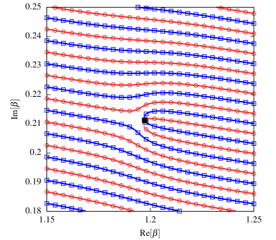
Figure 1: Map of the zeros of real (square) and imaginary (circle) parts of the partition function in the five-state clock model. The partition function is evaluated with the WL density of states sampled in the system of $L=16$. The Fisher zero is marked with the filled square.

II.2 Numerical strategies of finding the Fisher zeros

We follow a standard strategy of searching for partition function zeros that is usually evaluated with the reweighting scheme based on the Monte Carlo estimate of spectral densities Falcioni1982 ; Marinari1984 ; Ferrenberg1988 ; Ferrenberg1989 . Although the recipe is well known (for instance, see the procedures in Ref. Kenna1997 for Lee-Yang zeros and Alves1992 for Fisher zeros and references therein), let us briefly go through the implementation with the WL density of states for later discussion on the numerical uncertainty issue at the BKT transition given in Sec. III. The two-step procedures Alves1992 are composed of the graphical search to find an approximate location and the numerical minimization for refinement. As illustrated in Fig. 1, a map can be drawn for the zeros of the real and imaginary parts of the partition function $Z(\beta)$ in the plane of the complex inverse temperature $\beta\equiv\beta_{\mathrm{R}}+i\beta_{\mathrm{I}}$. This can be done by using a one-dimensional root finder for $\beta_{\mathrm{I}}$ at a given $\beta_{\mathrm{R}}$. Given the map in the wide range of $\beta_{\mathrm{R}}$, one can identify an approximate location of the crossing where the zeros of the real and imaginary parts meet each other. The leading Fisher zero $\beta_{1}$ is given by the crossing with the smallest magnitude of $\beta_{\mathrm{I}}$. Starting from the approximate location of the crossing, $\beta_{1}$ is refined by numerically minimizing $|Z(\beta)|$.

While this two-step approach can work in principle with any normalization of the partition function, the WL estimate may prefer the particular form with

$$\tilde{Z}(\beta)\equiv\frac{Z(\beta)}{Z(\beta_{\mathrm{R}})}=\sum_{E}P(E;\beta_{\mathrm{R}})e^{-i\beta_{\mathrm{I}}E}=\left\langle e^{-i\beta_{\mathrm{I}}E}\right\rangle_{\beta_{\mathrm{R}}}$$ (1)

because once the density of states $g(E)$ is obtained, the energy distribution $P(E;\beta_{\mathrm{R}})$ is computed straightforwardly at any real inverse temperature $\beta_{\mathrm{R}}$ as

$$P(E;\beta_{\mathrm{R}})\equiv\frac{1}{Z(\beta_{\mathrm{R}})}g(E)e^{-\beta_{\mathrm{R}}E}.$$ (2)

The energy distribution is not affected by an arbitrary normalization factor for the WL estimate of $g(E)\equiv g_{\mathrm{WL}}(E)$ since it is canceled out with $Z(\beta_{\mathrm{R}})$. The conventional MC simulations use a similar reweighting strategy in the grids of $\beta_{R}$. In the HOTRG calculations, the normalization is not relevant since it gives the direct computation of $\ln Z(\beta)$, but we will still consider $\tilde{Z}(\beta)$ for comparison with the WL estimates.

The other method to compute the partition function zeros is to use a polynomial solver, while it is applicable only when the density of states $g(E)$ is prepared as a function of equally spaced energy $E\equiv E_{n}$. For a given $E_{n}=n\epsilon+\epsilon_{0}$, where $n$ is a non-negative integer, one can find the zeros of the partition function by solving a complex polynomial equation,

$$Z(z)=e^{-\beta\epsilon_{0}}\sum_{n=0}^{n_{\mathrm{max}}}g_{n}z^{n}=0,$$ (3)

where $z\equiv\exp(-\beta\epsilon)$ and $g_{n}\equiv g(E_{n})$. The zeros can be computed for instance by using the MPSolve package mpsolve . This approach is applicable to the case of the Ising, Potts, and six-state clock models where the energy is regularly spaced. However, it cannot be used for the models with continuous symmetry like the $XY$ model or the ones with irregular energies like the five-state clock model without introducing an artificial binning error. For our purpose of discussing the vulnerability due to the MC noises in the zero finder, the two-step approach is also more intuitive. The leading zeros in this work are identified by using the two-step method.

II.3 Wang-Landau sampling method

The WL sampling method is used to estimate $g(E)$ in the Ising and Potts models. The standard algorithm Wang2001a ; Wang2001b is employed with the stopping criterion of the modification factor at $10^{-8}$. The histogram flatness criterion is set to be $0.99$ for the system sizes up to $L=32$ and $0.95$ for the larger systems.

The normalized partition function $\tilde{Z}(\beta)$ is evaluated based on a set of the WL samples of the density of states. The energy probability distribution in Eq. (2) is averaged over $N_{s}$ different WL samples of the density of states $\{g^{(k)}_{\mathrm{WL}}(E)\}$ as

$$P(E;\beta_{R})\approx\bar{P}_{\mathrm{WL}}(E;\beta_{R})=\frac{1}{N_{s}}\sum_{k=1}^{N_{s}}\frac{g^{(k)}_{\mathrm{WL}}(E)e^{-\beta_{R}E}}{\sum_{E^{\prime}}g^{(k)}_{\mathrm{WL}}(E^{\prime})e^{-\beta_{R}E^{\prime}}}.$$ (4)

We have $N_{s}=30$ from $30$ independent runs of the WL simulations for the model Hamiltonian examined. The measurement uncertainty of $\tilde{Z}(\beta)$ and the location of the leading zero are computed for the confidence level of 95% by repeating the bootstrap resampling processes $1000$ times with the prepared WL samples of the density of states.

On the other hand, in the $p$-state clock model, while we mainly use the HOTRG method in this work, the WL method was used for the Fisher zero problem in the previous studies Hwang2009 ; Kim2017 . However, the previous work Kim2017 reported the strong limitation in accessible system sizes and argued that it was due to a fundamental property of the Fisher zero at the BKT transition rather than the WL algorithm itself. In fact, for the six-state clock model, the WL density of states can be obtained for sizes up to $L=128$ within the same criterion used for the Ising model. Even larger systems can be considered by using the parallel algorithm Vogel2013 ; Vogel2014 . While the five-state clock model needs the two-parameter representation Kim2017 , advanced strategies for acceleration have been suggested recently for simulations in large systems Valentim2015 ; Ren2016 ; Chan2017a ; Chan2017b .

II.4 Higher-order tensor renormalization group

The HOTRG method Xie2012 provides a deterministic way of evaluating the partition function in the tensor-network representation. For a classical spin model with local interactions in the square lattices, the partition function can be written as

$$Z(\beta)=\mathrm{Tr}\exp(-\beta H)=\mathrm{Tr}\prod_{i}T_{x_{i}x^{\prime}_{i}y_{i}y^{\prime}_{i}},$$ (5)

where $T_{x_{i}x^{\prime}_{i}y_{i}y^{\prime}_{i}}$ represents a local tensor with the indices of four legs associated with the bonds in the $x$ and $y$ directions. The complexity in this product of the local tensors can be truncated systematically in a controlled way by using the real-space renormalization group procedures Levin2007 ; Xie2009 ; Zhao2010 ; Xie2012 . In particular, the HOTRG method has been extended to the study of the Fisher Denbleyker2014 and Lee-Yang GarciaSaez2015 zeros of the partition function evaluated at complex temperatures and fields.

Let us briefly review the HOTRG procedures. Initially, the model-dependent local tensor $T^{(0)}$ is prepared at each site, and then it is coarse-grained with the tensor in a neighboring site sharing a bond. In $2^{N}\times 2^{N}$ lattices, with translational invariance being assumed, it takes $2N$ operations of the contraction applied alternatively along the $x$ and $y$ directions to obtain the final coarse-grained tensor. For instance, the $n$th operation of the contraction along the $y$ direction starts by computing

$$M_{xx^{\prime}yy^{\prime}}^{(n)}=\sum_{i}T_{x_{1}x_{1}^{\prime}yi}^{(n)}T_{x_{2}x_{2}^{\prime}iy^{\prime}}^{(n)},$$ (6)

where $x=x_{1}\otimes x_{2}$ and $x^{\prime}=x_{1}^{\prime}\otimes x_{2}^{\prime}$. If the dimension of each leg of $T^{(n)}$ is $D$, then the dimension of $x$ and $x^{\prime}$ increases to $D^{2}$. The dimension of the legs will be exponentially large as the contraction goes on if $M_{xx^{\prime}yy^{\prime}}$ is given directly to the new tensor. This is prevented by introducing the cutoff dimension $D_{c}$ for the spectral truncation in the singular value decomposition. The truncation error is controlled by increasing $D_{c}$. The new coarse-grained tensor $T^{(n+1)}$ is then written as

$$T_{xx^{\prime}yy^{\prime}}^{(n+1)}=\sum_{ij}U_{ix}M_{ijyy^{\prime}}^{(n)}U_{jx^{\prime}}^{*}.$$ (7)

For a real $\beta$, a real unitary matrix $U$ can be obtained by solving the eigenproblem of the semi-positive-definite matrix $AA^{\dagger}$ with $A_{x,x^{\prime}yy^{\prime}}=M_{xx^{\prime}yy^{\prime}}$ or $A_{x^{\prime},xyy^{\prime}}=M_{xx^{\prime}yy^{\prime}}$, where the eigenvectors corresponding to the first $D_{c}$ largest eigenvalues are only taken to determine $U$. For a complex $\beta$, we follow the strategy proposed in the previous work for the $XY$ model Denbleyker2014 to find the orthogonal transformation with a real unitary matrix $U$. The previous work proposed to replace $AA^{\dagger}$ with $\mathrm{Re}[AA^{\dagger}]$, $\mathrm{Re}[AA^{T}]$, $\mathrm{Im}[AA^{\dagger}]$, or $\mathrm{Im}[AA^{T}]$. Here we choose $\mathrm{Re}[AA^{\dagger}]$ to preserve the trace of $AA^{\dagger}$ in our implementation of the HOTRG method. At every contraction, trying both of $A_{x,x^{\prime}yy^{\prime}}=M_{xx^{\prime}yy^{\prime}}$ and $A_{x^{\prime},xyy^{\prime}}=M_{xx^{\prime}yy^{\prime}}$ to build $AA^{\dagger}$, we pick the one with the smaller residue of the trace that is due to small eigenvalues not included in the largest $D_{c}$ eigenvalues constructing the new coarse-grained tensor $T^{(n+1)}$.

As the contractions are repeated, the components of $T^{(n)}$ can increase to very large numbers. To avoid the numerical overflow, we normalize $T^{(n)}$ by a factor of $\lambda_{n}$ which we set to be the Euclidean norm of $T^{(n)}$. After $2N$ steps of the contractions, the partition function is evaluated as

$$\ln Z=\ln\mathrm{Tr}\,\tilde{T}^{(2N)}+\sum_{i=1}^{2N}{2^{2N-i}}\ln{\lambda_{i}},$$ (8)

where $\tilde{T}^{(n)}\equiv T^{(n)}/\lambda_{n}$ is the normalized tensor.

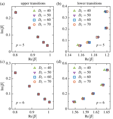
Figure 2: Leading zero identification compared between different values of the dimensional cutoff $D_{c}$ in the HOTRG procedures for the upper and lower transitions in the $p$-state clock model. The data points are available for the system sizes of $L=8,16,32,64,128$, where the smaller $L$ corresponds to the larger value of $\beta_{I}$.

The initial local tensor $T^{(0)}\equiv T$ depends on the model Hamiltonian. For the Ising and $q$-state Potts model, the exact expression of $T$ is known Zhao2010 ; Xie2012 ; Wang2014 . For the $p$-state clock model, we construct $T$ by using the same expansion technique previously used for the $XY$ model Yu2014 . The partition function $Z(\beta)$ of the $p$-state clock model is written as

$$Z(\beta)=\prod_{i}\sum_{\theta_{i}}\exp\Big{[}\beta\sum_{\langle i,j\rangle}\cos(\theta_{i}-\theta_{j})\Big{]}=\mathrm{Tr}\prod_{i}T_{x_{i}x^{\prime}_{i}y_{i}y^{\prime}_{i}}.$$ (9)

The Boltzmann factor can be expanded by using

$$e^{\beta\cos{\theta}}=\sum^{\infty}_{n=-\infty}I_{n}(\beta)e^{in\theta}\,,$$ (10)

where $I_{n}(\beta)$ is the modified Bessel function of the first kind. Summing out the spin angle variable $\theta_{i}$, we obtain

$$T_{xx^{\prime}yy^{\prime}}=\sqrt[]{I_{x}(\beta)I_{x^{\prime}}(\beta)I_{y}(\beta)I_{y^{\prime}}(\beta)}\delta_{\mathrm{mod}(x+y-x^{\prime}-y^{\prime},p),0}.$$ (11)

The difference from the $XY$ model is indicated by $\mathrm{mod}(x+y-x^{\prime}-y^{\prime},p)$, which is $x+y-x^{\prime}-y^{\prime}$ modulo $p$, appearing because of the discrete values of $\theta$. Note that the initial tensor can be prepared alternatively by using the singular value decomposition Chen2017 ; Chen2018 . While in the initial tensor, the magnitude of the coefficient $I_{n}(\beta)$ decays exponentially with increasing $n$, the cutoff dimension $D_{c}$ should be tested numerically for the required accuracy of final results. The $XY$ model was examined previously with $D_{c}=40$ and $50$ Yu2014 ; Denbleyker2014 . We increase the cutoff up to $D_{c}=70$, which is the largest $D_{c}$ available within our limitation of computational memory, for the identification of the leading zeros in the systems with sizes up to $L=128$ supp . Figure 2 displays the estimates with different $D_{c}$’s, indicating that $D_{c}=60$ and $70$ are very similar. We use the dataset of $D_{c}=70$ for the FSS analysis presented in later sections.

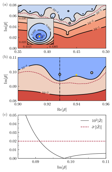
Figure 3: Landscape of the normalized partition function $|\tilde{Z}|$ evaluated with the WL density of states for (a) the Ising supp and (b) six-state clock models Kim2017 in the square lattices of $L=32$. The dashed lines in (a) and (b) indicate the boundary above which $|\tilde{Z}|$ is smaller than the uncertainty estimate $\tilde{\sigma}[|\tilde{Z}|]$. The location of the true leading zero obtained from the HOTRG calculations is marked with the filled star. (c) $|\tilde{Z}|$ and $\tilde{\sigma}[|\tilde{Z}|]$ plotted along the dash-dotted line in (b).

III Uncertainty of finding the leading zero under stochastic noises

The presence of stochastic noises is a general property of any MC estimator. The questions that we address in this section are how much one can trust the identification of the leading Fisher zero under the stochastic errors of the partition function estimate and how it depends on a particular character of the phase transition. These questions were briefly considered by one of us in the previous work Kim2017 which conjectured that based on the Gaussian approximation, the numerical tolerance to the noises is related to the critical behavior of the specific heat. We examine this conjecture beyond the Gaussian approximation by providing more detailed analysis with demonstrations in the Ising, Potts, and clock models.

III.1 System-size scaling of the uncertainty criterion

Figure 3 presents examples of reliable and unreliable identifications of the leading zeros in the presence of the stochastic uncertainty of the partition function estimate. Finding the zeros of the normalized partition function $\tilde{Z}(\beta)$ under the uncertainty should accompany with a test for a signal-to-noise ratio to lend confidence to the search for the zero. The minimal condition can be set for the “hill” of $|\tilde{Z}|$ surrounding the location of the zero to be higher than the uncertainty level [see the dashed line in Fig. 3(a)]; otherwise, the “valley” of $|\tilde{Z}(\beta)|=0$ is untrusted as indicated in Fig. 3(c). The boundary of confidence Alves1992 ; Denbleyker2007 ; Denbleyker2014 can be given by the measurements based on the WL dataset as a line above which the magnitude of $|\tilde{Z}(\beta)|$ is smaller than its uncertainty measure $\tilde{\sigma}[|\tilde{Z}(\beta)|]$.

While the boundary of confidence can be computed in MC simulations, one can build useful intuition about how the boundary would evolve with increasing system sizes from the analytic approach based on the Gaussian approximation of the energy distribution. In Ref. Alves1992 , the random sampling with the Gaussian energy distribution provided the standard error $\tilde{\sigma}[|\tilde{Z}(\beta)|]=[(1-|\tilde{Z}|^{2})/n_{s}]^{1/2}$, which defined the radius of confidence from the real axis as

$$R=\sqrt{\ln(n_{s}+1)}/\sigma_{E},$$ (12)

where $n_{s}$ is the size of the samples, and $\sigma_{E}^{2}\equiv\langle E^{2}\rangle-\langle E\rangle^{2}$ is the variance of energy at a given $\beta_{\mathrm{R}}$. The extension to the quasi-Gaussian distribution was also discussed in Ref. Denbleyker2007 . Despite the difference from realistic energy distributions, Eq. (12) still provides an important implication on the numerical accessibility to the leading zero that turns out to differ with the type of the associated phase transition.

The system-size dependence of $R$ is encoded in the energy variance that is proportional to the heat capacity. Since the heat capacity is extensive, one may anticipate that $R\sim L^{-d/2}$ in the $d$-dimensional lattices, indicating that the area where we can trust the estimate of $\tilde{Z}$ shrinks with a power law as $L$ increases. The decrease of $R$ is even faster in the vicinity of the leading zero along the line of $\beta_{\mathrm{R}}=\mathrm{Re}[\beta_{1}]$ because it corresponds to a pseudotransition point at which the specific heat $c_{L}^{*}$ becomes critical in the ordinary phase transition. However, an important missing piece in this argument is that the leading zero, which we want to identify, is also moving toward the real axis as the system size increases.

Therefore, what we need to consider is the race between $R(c_{L}^{*})$ and $\mathrm{Im}[\beta_{1}]$, both of which decrease with increasing $L$. If $R$ is always larger than $\mathrm{Im}[\beta_{1}]$ regardless of $L$, then one can successfully locate the leading zero even at a very large system within the uncertainty of the MC estimate. If $R$ becomes smaller than $\mathrm{Im}[\beta_{1}]$ at some point of $L$, then the zero identified under the noises is likely to be accidental and thus hardly trusted. Because $c_{L}^{*}$ and $\mathrm{Im}[\beta_{1}]$ are both governed by the critical behaviors, one may reach an intuition that while the FSS behavior of the leading zero characterizes the phase transition, the character of the transition may also influence reversely the numerical difficulty of finding the leading zero.

In the first-order transitions, the diverging specific heat $c_{L}^{*}\sim L^{d}$ at a pseudotransition point leads to $R\sim L^{-d}$ which coincides with the expected behavior of $\mathrm{Im}[\beta_{1}]\sim L^{-d}$. In the second-order transitions with the critical exponent $\alpha>0$, the specific heat $c_{L}^{*}\sim L^{\alpha/\nu}$ leads to $R\sim L^{-(d\nu+\alpha)/2\nu}$ that becomes $R\sim L^{-1/\nu}$ with the hyperscaling relation $d\nu=2-\alpha$, and the leading zero has the same scaling behavior of $\mathrm{Im}[\beta_{1}]\sim L^{-1/\nu}$. Therefore, the ordinary first-order and second-order transitions exhibit $R\sim\mathrm{Im}{\beta_{1}}$ regardless of $L$, suggesting that the leading zero may be marginally accessible even at a very large system under finite stochastic uncertainty of $|\tilde{Z}|$.

On the other hand, the situations are very different in the $XY$ model where the specific heat does not diverge Kosterlitz1973 ; Kenna1995 ; Kenna1997 ; Kenna2006 . The radius $R\sim L^{-d/2}$ decreases much faster than the imaginary part of the leading zero that is expected to scale as $\mathrm{Im}[\beta_{1}]\sim[\ln(bL)]^{-\tilde{q}}$ with $\tilde{q}=1+1/\nu$ at a very large $L$ Denbleyker2014 . The singular part of the specific heat with the logarithmic correction Kenna1995 ; Kenna1997 ; Kenna2006 is proportional to $L^{-d}(\ln L)^{2\tilde{q}}$ which is comparable to $\mathrm{Im}[\beta_{1}]^{-2}$; however, the main contribution to $R$ comes from the constant regular part since the singular part quickly decreases with increasing $L$. This leads to $R\ll\mathrm{Im}[\beta_{1}]$ at a large $L$, implying that for the BKT transitions, a reliable identification of the leading zero is fundamentally limited to small systems within the MC estimate of $|\tilde{Z}|$.

While Eq. (12) indicates a connection between the numerical feasibility of finding the leading zero and the critical phenomena, MC simulation are often performed to keep the measurement error at a certain level. Thus, in practice, it is meaningful to consider the criterion for a fixed uncertainty $\tilde{\sigma}_{0}$,

$$|\tilde{Z}(\beta)|\geq\tilde{\sigma}_{0},$$ (13)

which examines whether the hill of $|\tilde{Z}|$ surrounding the leading zero is visible above the uncertainty level Kim2017 . For the Gaussian energy distribution, $|\tilde{Z}(\beta)|$ at a complex value of $\beta=\beta_{\mathrm{R}}+i\beta_{\mathrm{I}}$ is calculated as

$$|\tilde{Z}(\beta)|=\exp\left[-L^{d}c_{L}^{*}\frac{\beta_{\mathrm{I}}^{2}}{2\beta_{\mathrm{R}}^{2}}\right].$$ (14)

At the location of the leading zero, $\beta=\beta_{1}$, the leading-order behavior of $|\tilde{Z}(\beta_{1})|\equiv Q(L)$ for a large $L$ can be written as

$$Q_{\mathrm{1st}}(L) = A_{L}\exp[-a_{0}L^{-d}],$$ (15)

$$Q_{\mathrm{2nd}}(L) = A_{L}\exp[-a_{0}L^{-\alpha/\nu}],$$ (16)

$$Q_{\mathrm{BKT}}(L) = A_{L}\exp[-a_{0}L^{d}(\ln bL)^{-2\tilde{q}}],$$ (17)

for the first-order, second-order, and BKT transitions, respectively, where a constant $a_{0}$ is given by the regular part of $c_{L}^{*}$. The singular part of $c_{L}^{*}$ is canceled out together with $\mathrm{Im}[\beta_{1}]$ as discussed for $R$. It contributes to to the factor $A_{L}$, but it may also contain the logarithmic or next-to-leading order corrections of $c_{L}^{*}$. For instance, in the Ising model, the specific heat with $\alpha=0$ diverges logarithmically as $c_{L}^{*}\sim\ln L$, leading to the power-law decay of $A_{L}$ as

$$Q_{\mathrm{Ising}}(L)=A_{0}L^{-a}.$$ (18)

For a small $\alpha$, considered the next-to-leading order correction term as in $c_{L}^{*}\sim L^{\alpha/\nu}(1-a_{\omega}L^{-\omega})$, we may rewrite $Q(\beta_{1})$ as

$$Q_{\mathrm{2nd}}(L)=A_{0}\exp[-a_{0}L^{-\alpha/\nu}+a_{1}L^{-\omega}],$$ (19)

indicating that $Q_{\mathrm{2nd}}(L)$ can decrease slowly as $L$ increases when $a_{0}<0$, or $a_{1}L^{-\omega}$ is positive and dominant.

Therefore, for the first-order transition, $Q_{\mathrm{1st}}$ is an increasing function of $L$, implying that the same uncertainty level is enough for large systems. While it works similarly in the second-order transition, one may need more accurate estimates at a larger system if $\alpha$ is small. For the BKT transitions, $Q_{\mathrm{BKT}}$ exponentially decays with increasing $L$, implying that a larger system requires exponentially more accurate estimates that may not be feasible with usual MC simulations.

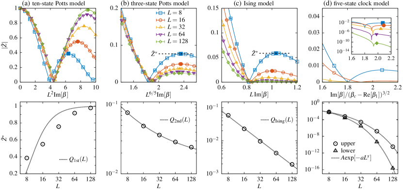
Figure 4: Numerical visibility of the leading zeros associated with the different types of phase transition. The normalized partition function $\tilde{Z}$ is plotted in the vicinity of the leading zero for (a) 10-state Potts, (b) three-state Potts, (c) Ising, and (d) five-state clock models. The hill height $\tilde{Z}^{*}$, the maximum of $|\tilde{Z}|$ above the leading zero in the imaginary axis is marked with a filled symbol. In the bottom panels, the system-size scaling behavior of $\tilde{Z}^{*}$ is compared with a curve fit to $Q(L)$ predicted from the Gaussian approximation. The partition functions shown here are obtained by using the WL density of states for the Ising and Potts models and by using the HOTRG method with $D_{c}=70$ for the five-state model. The identified location of the leading Fisher zeros are tabulated in Supplemental Material supp .

III.2 Numerical visibility of the leading zeros in spin models

A caveat of the above argument is that the Gaussian form of the energy distribution becomes a crude approximation near the actual location of the zero. It is well known that the Gaussian energy distribution cannot produce $Z=0$ as also indicated in Eq. (14). The previous work Kim2017 argued that Eq. (14) works as an envelope function of $\tilde{Z}(\beta)$, and thus the analytic connection between the numerical difficulty and the critical behavior of the specific heat can be still intuitive. Therefore, it is still important to check numerically, in the realistic spin models, how the maximally tolerable uncertainty for a trusted identification of the zero scales with the system size.

As illustrated in Fig. 3, the uncertainty level that can still reveal the valley of $|\tilde{Z}|=0$ is bound by the height of the hill surrounding the location of the zero. Thus, we compare the behavior of the hill height just above the leading zero, which we denote by $\tilde{Z}^{*}$, with the predicted scaling behavior of $Q(L)$. Figure 4 presents the system-size dependence of $\tilde{Z}^{*}$ in the Potts, Ising, and clock models to examine the different types of phase transition. The partition functions in the Potts and Ising models are evaluated based on the WL density of states, and the calculations are done in the clock model by using the HOTRG method. It turns out that despite the quantitative difference from $Q(L)$, the FSS behaviors of $\tilde{Z}^{*}(L)$ agree well with the behavior of $Q(L)$ predicted based on the Gaussian approximation of the energy distribution.

In the 10-state Potts model undergoing the first-order transition, it is notable that the estimate of $\tilde{Z}^{*}$ increases toward unity as $L$ increases [see Fig. 4(a)]. While the numerical data of $\tilde{Z}^{*}$ does not fit precisely to the line of $Q_{\mathrm{1st}}(L)$ in Eq. (15), the prediction of the increasing behavior is essentially valid. The excellent contrast between the hill and valley of $\tilde{Z}^{*}$ guarantees that the location of the leading zero can be accessible under finite noises even at a large system. The comparison with other phase transitions discussed below suggests that within the MC simulations, the numerical identification of the leading zero is the most stable at the first-order transition.

The examples of the second-order transitions also show excellent agreement with the expectation from the Gaussian approximation. The three-state Potts model shown in Fig. 4(b) presents that the hill height $\tilde{Z}^{*}$ decreases with $L$ but tends to asymptotically converges. The data points of $\tilde{Z}^{*}$ show a very good curve fit to $A\exp[-a_{0}L^{-\alpha/\nu}]$ with $a_{0}<0$ and $\alpha/\nu\approx 0.4$ given in Eq. (19). The parameters are consistent with the conjectured value of $\alpha/\nu=2/5$ denNijs1979 and the previous FSS test of the specific heat maximum where the negative constant term ($a_{0}<0$) was indicated Nagai2013 . In the Ising model presented in Fig. 4(c), the data points $\tilde{Z}^{*}$ indicate a power-law decrease as expected from $Q_{\mathrm{Ising}}(L)$ in Eq. (18). While the decreasing behavior suggests that the stochastic error should decrease accordingly to identify the leading zero, the measured uncertainty of our WL estimates is well below the hill level of $\tilde{Z}^{*}$ in the tested range of the system sizes.

On the other hand, in the five-state clock model, we observe an exponential decay of $\tilde{Z}^{*}\sim\exp(-aL^{x})$ in the HOTRG calculations of the partition function [see Fig. 4(d)]. This indicates that if there were finite noises, then the valley-hill structure around the leading zero would get exponentially less visible with increasing system size. Although the observed scaling behavior of $\tilde{Z}^{*}$ is different from Eq. (17), both reach the same conclusion that the search for the leading zero would become extremely vulnerable against stochastic noises, implying that the MC methods are inadequate to the Fisher-zero study of the BKT transitions. This emphasizes the advantage of HOTRG as a deterministic method whose accuracy is controlled with the cutoff dimension and free from stochastic noises.

In the next section, we present the FSS analysis with the leading zeros identified in the HOTRG calculations to characterize the BKT features of the upper and lower transitions in the five- and six-state clock models.

IV Two BKT transitions in the clock model

Let us begin this section by summarizing the problems that remain unsolved in the previous Fisher-zero study of the $p$-state clock model Kim2017 . First, for $p=5$, the transition point suggested by the leading zeros seemed to deviate from the previous estimates when the BKT exponent $\nu=1/2$ is used, while $\nu=1/2$ has been verified in the phenomenological FSS analysis Borisenko2011 and the analysis of the helicity modulus redefined for the discrete symmetry Kumano2013 ; Chatelain2014 . Second, the leading zeros at the lower transitions showed an arclike FSS trajectory which was different from the power-law trajectory expected from the $XY$ model. The leading zero behavior at the lower transition remains unexplained.

An obvious criticism to the previous analysis based on the WL density of states in Ref. Kim2017 was that the system sizes examined were too small to draw any conclusive results. Here we provide the FSS analysis with the leading zeros obtained by using the HOTRG calculations in the systems of sizes up to $L=128$. Nevertheless, it turns out that the finite-size effects are still strong so that the known leading-order ansatz is not enough to explain the observed behaviors, suggesting that subleading order corrections are necessary to be included in the FSS analysis within the available system sizes.

IV.1 Logarithmic correction to the finite-size-scaling ansatz

The FSS behavior of the leading Fisher zero in the previous study of the $XY$ model Denbleyker2014 was derived by extending the pseudotransition temperature obtained from the system-size scaling of the correlation length $\xi_{L}(\beta)\propto L$ into the domain of the complex temperature. It was found that a complex pseudotransition temperature $\beta_{L}\equiv\beta_{x}(L)+i\beta_{y}(L)$ would behave as $\beta_{y}\propto(\beta_{c}-\beta_{x})^{3/2}$ at a small $\beta_{y}$ at a large $L$. In the present study, we incorporate the logarithmic finite-size correction into the correlation length, which turns out to be essential to the FSS analysis of the leading Fisher zeros.

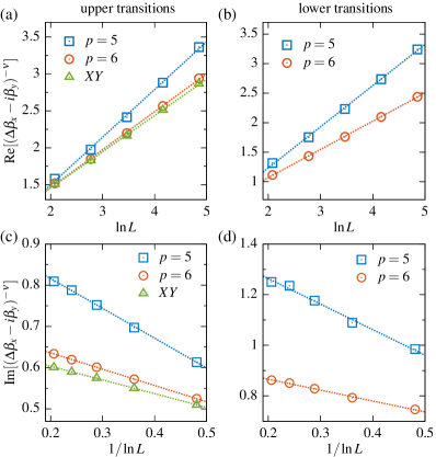
Figure 5: Logarithmic finite-size corrections to the scaling ansatz. The real and imaginary parts of $(\Delta\beta_{x}-i\beta_{y})^{-\nu}$ are shown at the transitions in the $p$-state clock model and the $XY$ model. The postulated BKT exponent $\nu=1/2$ is used. The dotted lines are given by the curve fits of the parameters in Eq. (22). The numerical values of the parameters are listed in Ref. supp . The HOTRG data at $D_{c}=70$ are used.

While the FSS ansatz of the correlation length is typically written as $\xi_{L}(\beta)/L=a_{0}$ with a constant $a_{0}$ for a large $L$, the previous MC study of the second moment correlation length in the $XY$ model Hasenbusch2005 indicated the presence of the logarithmic correction. Assumed that it works in the same way in the complex domain, we may begin with the ansatz written as

$$\frac{\xi_{L}(\beta)}{L}=a_{0}+\frac{a_{1}}{\ln L}+O[(\ln L)^{-2}],$$ (20)

where the constants $a_{0}$ and $a_{1}$ are complex numbers. Given the BKT ansatz of $\xi=A\exp[1/(at^{\nu})]$, we can write an equation for a reduced temperature $t\equiv t_{L}$ at a finite $L$ as

$$\frac{1}{at_{L}^{\nu}}=z_{0}+\ln L+\frac{z_{1}}{\ln L}+O[(\ln L)^{-2}],$$ (21)

where $z_{0}=\ln(a_{0}/A)$, and $z_{1}=a_{1}/a_{0}$. To the leading and next-to-leading orders for the real and imaginary parts of the right-hand side, the final FSS ansatz is written as

$$(\Delta\beta_{x}\pm i\beta_{y})^{-\nu}\simeq a\ln bL+i\left(c_{0}-\frac{c_{1}}{\ln L}\right),$$ (22)

where the complex reduced temperature $t_{L}$ for a transition point $\beta_{c}$ is written as $t_{L}\equiv\Delta\beta_{x}\pm i\beta_{y}$ with $\Delta\beta_{x}=|\beta_{c}-\beta_{x}|$. The sign of $\pm\beta_{y}$ is irrelevant because of the symmetry of the Fisher zero, and we choose $\beta_{y}>0$ and $t_{L}=\Delta\beta_{x}-i\beta_{y}$. The logarithmic behaviors of the real and imaginary parts are evident in the numerical tests with $\nu=1/2$ in Fig. 5.

Equation (22) can be solved for $\Delta\beta_{x}=r_{L}\cos\theta_{L}$ and $\beta_{y}=r_{L}\sin\theta_{L}$ in the polar coordinates of the complex inverse temperature. The radius $r_{L}$ and the angle $\theta_{L}$ are written as

$$r_{L} = (a\ln bL)^{-\frac{1}{\nu}}\left[1+\psi_{L}^{2}\right]^{-\frac{1}{2\nu}},$$ (23)

$$\theta_{L} = \frac{1}{\nu}\tan^{-1}\psi_{L},$$ (24)

where we define the size-dependent parameter $\psi_{L}$ as

$$\psi_{L}=\frac{1}{a\ln bL}\left[c_{0}-\frac{c_{1}}{\ln L}\right]\equiv\frac{\mathrm{Im}[(\Delta\beta_{x}-i\beta_{y})^{-\nu}]}{\mathrm{Re}[(\Delta\beta_{x}-i\beta_{y})^{-\nu}]}.$$ (25)

For a small $\psi_{L}$, one can write $\Delta\beta_{x}$ and $\beta_{y}$ as

$$\Delta\beta_{x} = (a\ln bL)^{-\frac{1}{\nu}}\left[1-B_{1}\psi_{L}^{2}+O(\psi_{L}^{4})\right],$$ (26)

$$\beta_{y} = \frac{1}{\nu}(a\ln bL)^{-\frac{1}{\nu}}\psi_{L}\left[1-B_{2}\psi_{L}^{2}+O(\psi_{L}^{4})\right],$$ (27)

where $B_{1}=\frac{1}{2\nu}+\frac{1}{2\nu^{2}}$, and $B_{2}=\frac{1}{3}+\frac{1}{2\nu}+\frac{1}{6\nu^{2}}$. One can further expand these equations in powers of $1/\ln L$ as

$$\Delta\beta_{x} \propto (\ln bL)^{-\frac{1}{\nu}}\left[1-B^{\prime}_{1}(\ln L)^{-2}+O[(\ln L)^{-3}]\right],$$ (28)

$$\beta_{y} \propto (\ln bL)^{-1-\frac{1}{\nu}}\left[1-B^{\prime}_{2}(\ln L)^{-1}+O[(\ln L)^{-2}]\right],$$ (29)

where $B^{\prime}_{1}=B_{1}c_{0}^{2}/a^{2}$, and $B^{\prime}_{2}=c_{1}/c_{0}$. In the asymptotic limit, they approach the lines of $\Delta\beta_{x}\propto(\ln bL)^{-1/\nu}$ and $\beta_{y}\propto(\ln bL)^{-1-1/\nu}$, reproducing the simple power-law trajectory of $\beta_{y}\propto\Delta\beta_{x}^{1+\nu}$ that was proposed in Ref. Denbleyker2014 . To take into account the logarithmic correction terms in $\Delta\beta_{x}$ and $\beta_{y}$, the leading zero trajectory can be expressed as

$$\Delta\beta_{x}=w_{1}\beta_{y}^{\frac{1}{1+\nu}}+w_{2}\beta_{y}+w_{3}\beta_{y}^{2-\frac{1}{1+\nu}}+O\big{(}\beta_{y}^{3-\frac{2}{1+\nu}}\big{)}\,,$$ (30)

where the coefficients can be determined perturbatively from the asymptotic solution. While this expression includes the higher-order corrections, it is still unclear how the trajectory can bend like an arc as previously observed at the lower transitions in the $p$-state clock model Kim2017 .

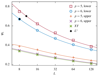
Figure 6: System-size dependence of $\psi_{L}$ in the $p$-state clock model and the $XY$ model. The solid lines indicate Eq. (25) with the fitting parameters determined in Fig. 5. The filled symbol denotes $L^{*}$ at which $\Delta\beta_{x}$ has maximum in Eq. (31).

We find that at the postulated BKT exponent $\nu=1/2$, the closed-form expressions of $\Delta\beta_{x}$ and $\beta_{y}$ are obtained to show more explicitly the character of the leading-zero trajectory at a finite $L$. At $\nu=1/2$, Eq. (22) provides the expressions,

$$\Delta\beta_{x} = \frac{\psi_{L}^{2}(1-\psi_{L}^{2})}{(1+\psi_{L}^{2})^{2}}\left[c_{0}-\frac{c_{1}}{\ln L}\right]^{-2},$$ (31)

$$\beta_{y} = \frac{2\psi_{L}^{3}}{(1+\psi_{L}^{2})^{2}}\left[c_{0}-\frac{c_{1}}{\ln L}\right]^{-2}.$$ (32)

It turns out that as $\psi_{L}$ decreases, $\Delta\beta_{x}$ increases first at a large $\psi_{L}$ and then starts to decrease when $\psi_{L}$ becomes smaller than a certain value. This contrasts with the monotonic increase in $\beta_{y}$. Thus, if $\psi_{L}$ is not small, then one may find $L^{*}$ at which the slope of $\Delta\beta_{x}$ change its sign, leading to an arclike trajectory in the complex plane. In the numerical tests shown in Fig. 6, the leading zeros at the lower transitions have much larger values of $\psi_{L}$ than at the upper transitions, explaining the strong finite-size effects observed at the lower transitions. Below we demonstrate the finite-size behaviors discussed in this section by using the HOTRG data of the leading zeros.

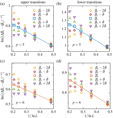
Figure 7: Determination of the transition points. The ansatz with the $1/\ln L$ correction is employed to locate the transition point $\beta_{c}$ at the upper [(a) and (c)] and lower [(b) and (d)] transitions in the $p$-state clock model. The sensitivity of the $1/\ln L$ behavior (solid line) is examined by moving away from $\beta_{c}$ with the step size $\delta=0.004$. The HOTRG data and the estimates of $\beta_{c}$ at $D_{c}=70$ are used.

IV.2 Finite-size-scaling behaviors of the leading Fisher zeros

The logarithmic FSS behavior in the imaginary part of Eq. (22) plays an essential role to determine the transition points from the leading Fisher zero data. While both of the real and imaginary parts expect the $\ln L$ dependence as shown in Fig. 5, the imaginary part of $(\Delta\beta-i\beta_{y})^{-\nu}$ responds much more sensitively to the change of $\beta_{c}$, providing a stable curve fit to locate $\beta_{c}$ in practice. Figure 7 demonstrates the behavior of $\mathrm{Im}[(\Delta\beta-i\beta_{y})^{-\nu}]$ with the postulated BKT exponent of $\nu=1/2$, indicating the systematic deviations of the data points from the straight line as it moves away from the determined value of $\beta_{c}$.

Table 1 lists our Fisher-zero estimates of $\beta_{c}$ based on the HOTRG data computed at $D_{c}=60$ and $70$ and the previous results based on various different measures at the upper and lower transitions in the $p$-state clock model for $p=5$ and $6$. Our estimates at both $D_{c}$’s are well in the range of the previous estimates. The estimate of $\beta_{c}$ is obtained by solving the least-squares problem to minimize the absolute difference between $\mathrm{Im}[\Delta\beta_{x}-i\beta_{y}]^{-1/2}$ and $c_{0}-c_{1}/\ln L$ in Eq. (22). The HOTRG calculations are deterministic and provide a single set of the leading Fisher zero data at each $D_{c}$ supp . The error given in the parentheses in Table 1 is the fitting uncertainty at a given $D_{c}$ measured by the jackknife variance with one data point being discarded. The fitting uncertainty gets smaller with the larger $D_{c}$, supporting the $1/\ln L$ correction ansatz in Eq. (22). Comparing with the previous Fisher zero study using the WL method Kim2017 , the reasons for the better agreement between the present results and the other estimates are twofold. First, our HOTRG dataset covers up to $L=128$ which is much larger than $L\lesssim 32$ of the previous WL study. Second, while Ref. Kim2017 relied on the form of the trajectory that is valid in the asymptotic limit, our method of locating $\beta_{c}$ benefits from the logarithmic finite-size correction in the next-to-leading order, providing a better access to finite systems at both of the upper and lower transitions.

The finite-size influence of neglecting the higher order logarithmic terms in the FSS ansatz of $(\Delta\beta_{x}-i\beta_{y})^{-\nu}$ can be tested by not including some data points of the smallest system sizes. Although our dataset of five data points is not enough for a systematic analysis, we can still compare the one from the full dataset with the other from the reduced dataset excluding $L=8$. As shown in Table 1, the locations of $\beta_{c}$ at the upper transitions are stable with the exclusion of $L=8$. At the lower transitions, the finite-size effect is much stronger as suggested by the test of $\psi_{L}$ in Fig. 6, however the change of $\beta_{c}$ is still in the range of the values reported in the previous studies. In addition, the same procedures provides $\beta_{c}\approx 1.115$ in the $XY$ model for our leading-zero dataset of $L\leq 128$, which is also comparable to the high-precision estimate $\beta_{c}\approx 1.1199$ given by the large-scale MC simulations Hasenbusch2005 ; Komura2012 .

Table 1: Comparisons with the previous estimates of the transition points for the upper ($\beta_{c}^{\mathrm{high}}$) and lower ($\beta_{c}^{\mathrm{low}}$) transitions in the $p$-state clock model. The last four rows indicate our estimates from the fits to Eq. (22) with the HOTRG dataset for $L\geq L_{\mathrm{min}}$ at $D_{c}=60$ and $70$.

$\beta_{c}^{\mathrm{high}}$($p=5$)	$\beta_{c}^{\mathrm{low}}$($p=5$)	$\beta_{c}^{\mathrm{high}}$($p=6$)	$\beta_{c}^{\mathrm{low}}$($p=6$)	reference
		1.088(12)	1.47(4)	Challa1986
		1.1111	1.4706	Yamagata1991
		1.1101(7)	1.4257(22)	Tomita2002
1.0510(10)	1.1049(10)			Borisenko2011
		1.1086(6)		Baek2013
1.0593	1.1013	1.106(6)	1.4286(82)	Kumano2013
1.058(19)	1.094(14)			Chatelain2014
1.0504(1)	1.1075(1)			Chen2018
				$D_{c}=60$
1.060(2)	1.097(3)	1.110(6)	1.436(6)	$L_{\mathrm{min}}=8$
1.058(2)	1.096(16)	1.114(15)	1.433(20)	$L_{\mathrm{min}}=16$
				$D_{c}=70$
1.059(1)	1.096(7)	1.106(1)	1.441(5)	$L_{\mathrm{min}}=8$
1.058(1)	1.101(6)	1.106(2)	1.444(2)	$L_{\mathrm{min}}=16$

Figure 8: Finite-size-scaling behaviors of the leading zeros at the transitions in the $p$-state clock model and the $XY$ model. The imaginary [(a) and (b)] and real [(c) and (d)] parts of the leading zeros and their trajectory in the complex plane [(e) and (f)] are examined at the upper [(a), (c), and (e)] and lower [(b), (d) and (f)] transitions. The dotted lines indicates Eqs. (31) and (32). The trajectories at the lower transitions are rescaled with the factor $r_{p}\equiv 1-\cos{(2\pi/p)}$ for visualization. The data at $D_{c}=70$ and the parameters determined from Fig. 5 are used.

The imaginary and real part of the leading zeros are expected to behave as $\beta_{y}\sim(\ln bL)^{-1-1/\nu}$ and $\Delta\beta_{x}\sim(\ln bL)^{-1/\nu}$ from the BKT ansatz in the limit of a very large $L$. While at a finite $L$, the leading zero behaviors deviate from these asymptotes, Eqs. (31) and (32) that include the finite-size corrections describe very well the FSS behaviors of the leading zeros, including an arclike trajectory at the lower transition, as demonstrated in Fig. 8. The parameters in $\psi_{L}$ are determined from the linear fits shown in Fig. 5 in the procedures of locating $\beta_{c}$. The excellent agreement between the data points and the analytic predictions again emphasizes that the logarithmic correction to the BKT ansatz is essential to the analysis of the leading zeros in the $p$-state clock model.

Finally, let us discuss briefly the BKT exponent $\nu$ that is fixed at the standard value of $\nu=1/2$ in our FSS tests. While it is hard to determine $\nu$ directly from $\Delta\beta_{x}$ or $\beta_{y}$ because of other fitting parameters being involved, the asymptote of the leading zero trajectory, $\beta_{y}\propto\Delta\beta_{x}^{1+1/\nu}$, can be checked for the consistency with the HOTRG data because it is free from the parameters other than the estimate of $\beta_{c}$. It turns out that at the upper transition, where the finite-size influence is less pronounced, the leading zero data agree very well with the prediction of $\beta_{y}\propto\Delta\beta_{x}^{3/2}$ as shown in Fig. 8(e). At the lower transitions, while the finite-size influence is much stronger as shown in Fig. 8(f), the extrapolation of the leading-zero data points is getting closer to the asymptotic behavior of $\nu=1/2$ as $L$ increases, suggesting that the lower transitions as well as the upper ones are indeed of the same BKT type yet with the different appearance of the finite-size effects.

V Summary and conclusions

We have investigated the numerical feasibility of the FSS analysis with leading Fisher zeros for the BKT transitions and proposed the logarithmic corrections to the FSS ansatz to examine the two phase transitions in $p$-state clock models for $p=5$ and $6$ in the square lattices. Our main findings can be summarized in two parts. (i) The reliability of the leading zero identification under finite MC noises highly depends on the type of the associated phase transition. (ii) The combination of the HOTRG method and the logarithmic correction to the FSS ansatz allows us to locate the transition points, resolving the discrepancy between the previous Fisher zero study and the other estimates from different measures.

We have found that the numerical visibility of the leading zero exhibits the characteristic system-size scaling that depends on the type of phase transition. The analytic prediction and the numerical tests in the Potts, Ising, and clock model suggest that the leading zero identification is the most robust against the finite MC noises in the first-order transition. In the second-order transition with a non-negative specific heat exponent, the tolerance to the finite noises decreases slowly with increasing system size. In the BKT transition, the tolerance decay turns out to be exponential, emphasizing the necessity of an highly accurate partition function evaluation in the search for the leading zero.

Employing the deterministic HOTRG method, we have identified the leading zeros for system sizes up to $L=128$ in the $p$-state clock model. Although, it turns out that the logarithmic correction is essential to the characterization of the leading zero behavior. The logarithmic correction works as a guide to locate the transition points, providing the Fisher-zero estimates that are in good agreement with the other estimates from different measures. In addition, our formulation of the FSS ansatz indicates that an arclike trajectory of the leading Fisher zeros can occur if the finite-size influence is strong as indeed observed at the lower transitions. Our results significantly extend the previous Fisher zero studies of the $p$-state clock model Hwang2009 ; Kim2017 by describing both of the upper and lower transitions within the same BKT scaling ansatz of the leading zeros with the finite-size correction.

- (1) Finite-size Scaling, edited by J. L. Cardy (North-Holland, Amsterdam, 1988).
- (2) M. E. Fisher, in Critical Phenomena, Vol. 51 of Proceedings of the “Enrico Fermi” International School of Physics, edited by M. S. Green (Academic Press, New York, 1971).
- (3) M. E. Fisher and M. N. Barber, Phys. Rev. Lett. 28, 1516 (1972).
- (4) B. Berche, R. Kenna, and J.-C. Walter, Nucl. Phys. B 865, 115 (2012).
- (5) R. Kenna and B. Berche, Condens. Matter Phys. 16, 23601 (2013).
- (6) R. Kenna and B. Berche, in Order, Disorder and Criticality, edited by Y. Holovatch (World Scientific, Singapore, 2015), Vol. 4, chap. 1.
- (7) V. L. Berezinskii, Zh. Eksp. Teor. Fiz. 59, 907 (1971); [Sov. Phys. JETP 32, 493 (1971)].
- (8) J. M. Kosterlitz and D. Thouless, J. Phys. C 5, L214 (1972).
- (9) J. M. Kosterlitz and D. Thouless, J. Phys. C 6, 1181 (1973).
- (10) I. Bena, M. Droz, and A. Lipowski, Int. J. Mod. Phys. B 19, 4269 (2005).
- (11) C. N. Yang and T. D. Lee, Phys. Rev. 87, 404 (1952).
- (12) M. E. Fisher, in Lectures in Theoretical Physics, edited by W. E. Brittin (University of Colorado Press, Boulder, 1965), Vol. 7C, chap. 1.
- (13) W. Janke and R. Kenna, J. Stat. Phys. 102, 1211 (2001).
- (14) R. Kenna and A. C. Irving, Phys. Lett. B 351, 273 (1995).
- (15) A. C. Irving and R. Kenna, Phys. Rev. B 53, 11568 (1996).
- (16) R. Kenna and A. C. Irving, Nucl. Phys. B 485, 583 (1997).
- (17) A. Denbleyker, Y. Liu, Y. Meurice, M. P. Qin, T. Xiang, Z. Y. Xie, J. F. Yu, and H. Zou, Phys. Rev. D 89, 016008 (2014); H. Zou, Ph.D. thesis, University of Iowa (2014).
- (18) J. C. S. Rocha, L. A. S. Mól, and B. V. Costa, Comput. Phys. Commun. 209, 88 (2016).
- (19) B. V. Costa, L. A. S. Mól, and J. C. S. Rocha, Comput. Phys. Commun. 216, 77 (2017).
- (20) C.-O. Hwang, Phys. Rev. E 80, 042103 (2009).
- (21) D.-H. Kim, Phys. Rev. E 96, 052130 (2017).
- (22) F. Wang and D. P. Landau, Phys. Rev. Lett. 86, 2050 (2001).
- (23) F. Wang and D. P. Landau, Phys. Rev. E 64, 056101 (2001).
- (24) N. A. Alves, J. P. N. Ferrite, and U. H. E. Hansmann, Phys. Rev. E 65, 036110 (2002).
- (25) R. Kenna, Condens. Matter Phys. 9, 283 (2006).
- (26) M. Hasenbusch, J. Phys. A: Math. Gen. 38, 5869 (2005).
- (27) Y. Komura and Y. Okabe, J. Phys. Soc. Jpn. 81, 13001 (2012).
- (28) R. Kenna, D. A. Johnston, and W. Janke, Phys. Rev. Lett 96, 115701 (2006).
- (29) R. Kenna, D. A. Johnston, and W. Janke, Phys. Rev. Lett. 97, 155702 (2006).
- (30) R. Kenna, in Order, Disorder and Criticality, edited by Y. Holovatch (World Scientific, Singapore, 2013), Vol. 3, chap. 1.
- (31) 40 Years of Berezinskii-Kosterlitz-Thouless Theory, edited by J. V. José (World Scientific, London, 2013).
- (32) S. Elitzur, R. B. Pearson, and J. Shigemitsu, Phys. Rev. D 19, 3698 (1979).
- (33) J. L. Cardy, J. Phys. A: Math. Gen. 13, 1507 (1980).
- (34) M. B. Einhorn, R. Savit, and E. Rabinovici, Nucl. Phys. B 170, 16 (1980).
- (35) C. J. Hamer and J. B. Kogut, Phys. Rev. B 22, 3378 (1980).
- (36) J. Fröhlich and T. Spencer, Comm. Math. Phys. 81, 527 (1981).
- (37) B. Nienhuis, J. Stat. Phys. 34, 731 (1984).
- (38) G. Ortiz, E. Cobanera, and Z. Nussinov, Nucl. Phys. B 854, 780 (2012).
- (39) J. Tobochnik, Phys. Rev. B 26, 6201 (1982); 27, 6972 (1983).
- (40) M. S. S. Challa and D. P. Landau, Phys. Rev. B 33, 437 (1986).
- (41) A. Yamagata and I. Ono, J. Phys. A: Math. Gen. 24, 265 (1991).
- (42) Y. Tomita and Y. Okabe, Phys. Rev. B 65, 184405 (2002).
- (43) O. Borisenko, G. Cortese, R. Fiore, M. Gravina, and A. Papa, Phys. Rev. E 83, 041120 (2011).
- (44) O. Borisenko, V. Chelnokov, G. Cortese, R. Fiore, M. Gravina, and A. Papa, Phys. Rev. E 85, 021114 (2012).
- (45) C. M. Lapilli, P. Pfeifer, and C. Wexler, Phys. Rev. Lett. 96, 140603 (2006).
- (46) S. K. Baek, P. Minnhagen, and B. J. Kim, Phys. Rev. E 81, 063101 (2010).
- (47) S. K. Baek, P. Minnhagen, Phys. Rev. E 82, 031102 (2010).
- (48) S. K. Baek, H. Mäkelä, P. Minnhagen, and B. J. Kim, Phys. Rev. E 88, 012125 (2013).
- (49) Y. Kumano, K. Hukushima, Y. Tomita, and M. Oshikawa, Phys. Rev. B 88, 104427 (2013).
- (50) C. Chatelain, J. Stat. Mech. (2014) P11022.
- (51) J. Chen, H.-J. Liao, H.-D. Xie, X.-J. Han, R.-Z. Huang, S. Cheng, Z.-C. Wei, Z.-Y. Xie, and T. Xiang, Chin. Phys. Lett. 34, 050503 (2017).
- (52) Y. Chen, Z.-Y. Xie, and J.-F. Yu, Chin. Phys. B 27, 080503 (2018).
- (53) T. Surungan, S. Masuda, Y. Komura, and Y. Okabe, J. Phys. A: Math. Theor. 52, 275002 (2019).
- (54) M. Falcioni, E. Marinari, M. L. Paciello, G. Parisi, and B. Taglienti, Phys. Lett. B 108, 311 (1982).
- (55) E. Marinari, Nucl. Phys. B 235, 123 (1984).
- (56) A. M. Ferrenberg and R. H. Swendsen, Phys. Rev. Lett. 61, 2635 (1988).
- (57) A. M. Ferrenberg and R. H. Swendsen, Phys. Rev. Lett. 63, 1195 (1989).
- (58) N. A. Alves, B. A. Berg, and S. Sanielevici, Nucl. Phys. B 376, 218 (1992).
- (59) D. A. Bini and L. Robol, J. Comput. Appl. Math. 272, 276 (2014).
- (60) T. Vogel, Y. W. Li, T. Wüst, and D. P. Landau, Phys. Rev. Lett. 110, 210603 (2013).
- (61) T. Vogel, Y. W. Li, T. Wüst, and D. P. Landau, Phys. Rev. E 90, 023302, (2014).
- (62) A. Valentim, J. C. S. Rocha, S.-H. Tsai, Y. W. Li, M. Eisenbach, C. E. Fiore, and D. P. Landau, J. Phys.: Conf. Ser. 640, 012006 (2015).
- (63) Y. Ren, S. Eubank, and M. Nath, Phys. Rev. E 94, 042125 (2016).
- (64) C. H. Chan, G. Brown, and P. A. Rikvold, Phys. Rev. E 95, 053302 (2017).
- (65) C. H. Chan, G. Brown, and P. A. Rikvold, Phys. Rev. B 96, 174428 (2017).
- (66) Z. Y. Xie, J. Chen, M. P. Qin, J. W. Zhu, L. P. Yang, and T. Xiang, Phys. Rev. B 86, 045139 (2012).
- (67) M. Levin and C. P. Nave, Phys. Rev. Lett. 99, 120601 (2007).
- (68) Z. Y. Xie, H. C. Jiang, Q. N. Chen, Z. Y. Weng, and T. Xiang, Phys. Rev. Lett. 103, 160601 (2009).
- (69) H. H. Zhao, Z. Y. Xie, Q. N. Chen, Z. C. Wei, J. W. Cai, and T. Xiang, Phys. Rev. B 81, 174411 (2010).
- (70) A. García-Saez and T.-C. Wei, Phys. Rev. B 92, 125132 (2015).
- (71) S. Wang, Z.-Y. Xie, J. Chen, B. Normand, and T. Xiang, Chin. Phys. Lett. 31, 070503 (2014).
- (72) J. F. Yu, Z. Y. Xie, Y. Meurice, Y. Liu, A. Denbleyker, H. Zou, M. P. Qin, J. Chen, and T. Xiang, Phys. Rev. E 89 013308 (2014).
- (73) See Supplemental Material for the table of the numerical data of the leading zeros identified.
- (74) A. Denbleyker, D. Du, Y. Meurice, and A. Velytsky, Phys. Rev. D 76, 116002 (2007).
- (75) M. P. M. den Nijs, J. Phys. A, 12, 1857 (1979).
- (76) T. Nagai, Y. Okamoto, and W. Janke, Condens. Matter Phys. 16, 23605 (2013).