Knot Topology in Quantum Spin System

Abstract

Knot theory provides a powerful tool for the understanding of topological matters in biology, chemistry, and physics. Here knot theory is introduced to describe topological phases in the quantum spin system. Exactly solvable models with long-range interactions are investigated, and Majorana modes of the quantum spin system are mapped into different knots and links. The topological properties of ground states of the spin system are visualized and characterized using crossing and linking numbers, which capture the geometric topologies of knots and links. The interactivity of energy bands is highlighted. In gapped phases, eigenstate curves are tangled and braided around each other forming links. In gapless phases, the tangled eigenstate curves may form knots. Our findings provide an alternative understanding of the phases in the quantum spin system, and provide insights into one-dimension topological phases of matter.

Introduction.—Knots are categorized in terms of geometric topology, and describe the topological properties of one-dimensional (1D) closed curves in a three-dimensional space KnotTheory ; AB . A collection of knots without an intersection forms a link. The significance of knots in science is elusive; however, knot theory can be used to characterize the topologies of the DNA structure DNA and synthesized molecular structure Forgan in biology and chemistry. Knot theory is used to solve fundamental questions in physics ranging from microscopic to cosmic textures and from classical mechanics to quantum physics Wilczek ; Rovelli ; CNYang ; FYWu ; Atiyah ; VK ; Faddeev ; Kauffman . Knots and links are observed for vortices in fluids Irvine13 ; Irvine16 , lights Leach ; Dennis , and quantum eigenfunctions Taylor , for solitons in the Bose–Einstein condensate Hall , and for Fermi surfaces of topological semimetals in Hermitian SCZhang ; JMHou ; ZWang ; ZYan ; Ezawa ; PYChang ; Ackerman ; DLD1 ; DLD2 ; LLu18 ; JHu19 and non-Hermitian systems JHuPRB ; Bergholtz1 ; Bergholtz2 ; CHLee . Knots and links with distinctive geometric topological features are crucial for understanding hidden physics.

Innovations in visualization have driven scientific developments. Historically, Feynman diagrams are created to provide a convenient approach for describing and calculating complex physical processes in quantum theory Feynman . Feynman diagrams help to understanding the interaction between particles and provide a thorough understanding of the foundations of quantum physics. In condensed matter physics, a coherent description of matter is difficult because of the complexity of its phases. In 1D topological systems, the phases of matter are generally characterized using a winding number associated with a Zak phase of the corresponding band. Topological phases with different winding numbers are considerably different from each other, and differences in their topological properties can be attributed to the eigenstates. The winding numbers and Zak phases are defined for separate energy bands. In the gapless phase, the boundaries of different gapped phases should have different topological features; however, the energy band is inseparable. The compatible characterization of gapped and gapless phases is a concern.

In this Letter, a graphic approach was developed to examine topological properties and phase transitions in 1D topological systems. The ground states of the quantum spin system are mapped into knots and links; the topological invariants constructed from eigenstates are then directly visualized; and topological features are revealed from the geometric topologies of knots and links. In contrast to the conventional description of band topologies, such as the Zak phase and Chern number that can be extracted from a single band, this approach highlights the interactivity between upper and lower bands; thus, information on two bands is necessary for obtaining a complete eigenstate graph. Several standard processes have been performed to diagonalize the Hamiltonian of the quantum spin system. The spin-$1/2$ is transformed into a spinless fermion under the Jordan-Wigner transformation. In Majorana representation, the core matrix of the spinless fermion system is obtained under Nambu representation. The eigenstates of the core matrix are then mapped into closed curves of knots and links. The graphs of different categories represent different topological phases.

To exhibit various topological phases, an exactly solvable generalized $XY$ model with long-range interactions is revisited, which ensures the richness of topological phases GZhang . The closed curves of eigenstates completely encode the information on ground states. In topologically nontrivial phases, eigenstate curves are tangled to form links for the gapped phase; however, they may be untied and combined into knots for the gapless phase. Because the winding number (Zak phase) is not appropriately defined in the gapless phase, knot theory KnotTheory is employed to characterize the topological features of both gapped and gapless phases. In this approach, the gapped and gapless phases are visualized, and their topological features are revealed through knots and links.

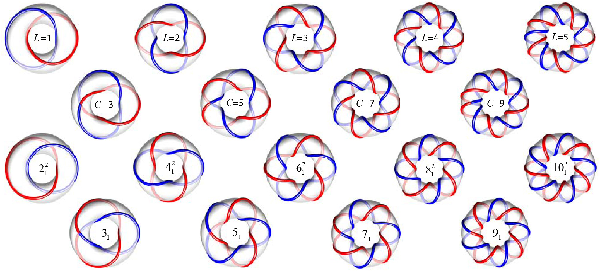
Figure 1: The upper (lower) two rows are eigenstate knots and links on the $k$-$\varphi$ torus with positive (negative) crossing and linking numbers. The first and third rows are the links, the second and fourth rows are the knots. The numbers in the lower two rows indicate the crossing number, and the superscript represents the number of loops, which is absent for the single loop knots. The subscript indicates the order of knot configuration with an identical number of loops and an identical crossing number in the Alexander-Briggs notation AB . The parameters in Eq. (10) for the $18$ knots and links from left to right and from top to bottom are $(x,y)$=$(1.1,1.2)$, $(0.5,1.2)$, $(0,1.2)$, $(-0.5,1.2)$, $(-0.8,1.2)$; $(0.68,1.2)$, $(0.28,1.2)$, $(-0.28,1.2)$, $(-0.68,1.2)$; $(2,0.7)$, $(1.8,0)$, $(1.8,-0.5)$, $(1.8,-1)$, $(1.8,-1.5)$; $(2,0.21)$, $(1.5,-0.32)$, $(2,-0.75)$, $(2,-1.2)$.

Quantum spin model.—A solvable generalized 1D $XY$ model with long-range three-spin interactions is considered for elucidation Suzuki . The Hamiltonian is

$$H=\sum\limits_{j=1}^{N}[\sum\limits_{n=1}^{M}\left(J_{n}^{x}\sigma_{j}^{x}\sigma_{j+n}^{x}+J_{n}^{y}\sigma_{j}^{y}\sigma_{j+n}^{y}\right)\prod_{l=j+1}^{j+n-1}\sigma_{l}^{z}+g\sigma_{j}^{z}],$$ (1)

where operators $\sigma_{j}^{x,y,z}$ are Pauli matrices for spin at the $j$th site. $H$ is reduced to an ordinary anisotropic $XY$ model for $M=1$. A conventional Jordan-Wigner transformation for spin-$1/2$ is performed Sachdev , and the Hamiltonian of a subspace with odd number particles can be expressed using a Hamiltonian describing a spinless fermion as follows

$$H=\sum\limits_{j=1}^{N}[\sum\limits_{n=1}^{M}(J_{n}^{+}c_{j}^{{\dagger}}c_{j+n}+J_{n}^{-}c_{j}^{{\dagger}}c_{j+n}^{{\dagger}}+\mathrm{H.c.})+g(1-2c_{j}^{\dagger}c_{j})],$$ (2)

where $c_{j}^{\dagger}$ ($c_{j}$) denotes the creation (annihilation) operator of spinless fermion at the $j$th site and $J_{n}^{\pm}=J_{n}^{x}\pm J_{n}^{y}$. In large $N$ limit ($N\gg M$), $H$ is available for both parities of particle numbers, thus representing a $p$-wave topological superconducting wire using long-range interactions kitaev ; Niu . Majorana fermion operators are introduced, $a_{j}=c_{j}^{\dagger}+c_{j},b_{j}=-i(c_{j}^{\dagger}-c_{j})$, the inverse transformation gives $c_{j}^{\dagger}=\left(a_{j}+ib_{j}\right)/2,c_{j}=\left(a_{j}-ib_{j}\right)/2$. The Majorana representation of the Hamiltonian is

$$H=i\sum\limits_{j=1}^{N}[\sum\limits_{n=1}^{M}\left(J_{n}^{x}b_{j}a_{j+n}-J_{n}^{y}a_{j}b_{j+n}\right)+ga_{j}b_{j}].$$ (3)

In the Nambu representation of basis $\psi^{\mathrm{T}}=(a_{1}$, $ib_{1}$, $a_{2}$, $ib_{2}$, $...)$, $H=\psi^{\mathrm{T}}h\psi$ and $h$ is a $2N\times 2N$ matrix. Applying Fourier transformation, we obtain $h=\sum_{k}h_{k}$ and

$$h_{k}=B_{x}\sigma_{x}+B_{y}\sigma_{y}\mathbf{,}$$ (4)

where $\sigma_{x}=\left(\begin{array}[]{cc}0&1\\ 1&0\end{array}\right)$ and $\sigma_{y}=\left(\begin{array}[]{cc}0&-i\\ i&0\end{array}\right)$. The components of the effective magnetic field are periodic functions of momentum $k$

$$B_{x}=\sum\limits_{n=1}^{M}J_{n}^{+}\cos\left(nk\right)/4-g/4,B_{y}=\sum\limits_{n=1}^{M}J_{n}^{-}\sin\left(nk\right)/4,$$ (5)

all information on the system is encoded in matrix $h_{k}$, because the eigenvalues and eigenvectors can be employed to construct the complete eigenstates of the original Hamiltonian. A winding number is defined using an effective planar magnetic field $\left(B_{x},B_{y}\right)$ as follows

$$w=\frac{1}{2\pi}\oint_{C}\mathbf{(}\hat{B}_{x}\nabla\hat{B}_{y}-\hat{B}_{y}\nabla\hat{B}_{x}),$$ (6)

where $\hat{B}_{x(y)}=B_{x(y)}/B$, $B=\left(B_{x}^{2}+B_{y}^{2}\right)^{1/2}$, and $C$ is the Bloch vector curves in the $B_{x}$-$B_{y}$ plane. $w$ characterizes a vortex enclosed in the loop. In the gapless phase, loop $C$ passes through the origin, and integral $w$ depends on the loop path. Although $w$ is crucial for characterizing the gapped phase, $w$ cannot be used to characterize the gapless phase (see Supplementary Material A SI ).

To overcome this concern, a graphic representation is developed to visualize the eigenstates (Fig. 1). The eigenstates in different gapless and gapped phases are mapped into different categories of torus knots and links. The topological features of the ground state are evident through the geometric topologies of eigenstate knots and links on $k$-$\varphi$ torus. Therefore, knot theory in mathematics can characterize topology phases in physics. The obtained knots and links depend on Fourier transformation. However, different topological phases are still distinguishable in the graphic representation; moreover, $h_{k}$ and knots are unique for the set Fourier transformation. In the following sections, we discuss the graphic eigenstate, topological characterization, and knot theory for the topological phases of the quantum spin system.

The spectrum of $h_{k}$ is $\epsilon_{k}^{\pm}=\pm B$ and the corresponding eigenstate is $\left|\psi_{k}^{\pm}\right\rangle=[e^{i\varphi_{\pm}(k)},1]^{\mathrm{T}}/\sqrt{2}$. The phases in eigenstate $\left|\psi_{k}^{\pm}\right\rangle$ are real periodic functions of $k$, $\varphi_{+}(k)=\arctan\left(-B_{y}/B_{x}\right)$, and

$$\varphi_{-}(k)=\varphi_{+}(k)+\pi.$$ (7)

The ground state phase diagram is obtained using $\epsilon_{k_{c}}^{\pm}=0$, where the energy band gap closes.

Knot topology.—The topological features of the ground state are completely encoded in phase factor $\varphi_{\pm}(k)$. In the absence of band degeneracy, the energy bands are gapped and each eigenstate is represented as a closed curve on the surface of an unknotted torus in $\mathbf{R}^{3}$. The toroidal direction is $k$ and the poloidal direction is $\varphi$ (Fig. 1). From $\varphi_{-}(k)=\varphi_{+}(k)+\pi$, the two curves are always located at opposite points in the cross section of the torus. For topologically nontrivial phases, they become tangled curves, which are braided around each other. In the presence of band degeneracy, two eigenstates may form one closed curve. The topological properties of the ground state are reflected from the geometric topology of closed curves. The curves on the torus forms a torus knot, which is a particular type of knots/links on the surface of an unknotted torus KnotTheory . For the eigenstate graphs of the corresponding quantum spin system, eigenstate graphs are only single-loop knots and two-loop links. The rich topological phases of either gapless or gapped, either Hermitian or non-Hermitian band degeneracy, and either trivial or nontrivial phases are all distinguishable from the eigenstate graphs. The graphic approach is employed to distinguish between the real gapless phases arising from exceptional points and degenerate points, which cannot be distinguished using the two winding numbers in the non-Hermitian system YXM .

For a gapped system, the two loops without any node form a link on the torus. In knot theory, for the topology of the two closed curves (loops) in the three-dimensional space, a linking number is used as a topological invariant Alexander . The linking number represents the number of times each curve is braided around the other curve. Mathematically, the linking number of two closed curves $\mathbf{r}_{+}(k)$ and $\mathbf{r}_{-}(k^{\prime})$ can be calculated using a double line integral

$$L=\frac{1}{4\pi}\oint\nolimits_{k}\oint\nolimits_{k^{\prime}}\frac{\mathbf{r}_{+}(k)-\mathbf{r}_{-}(k^{\prime})}{\left|\mathbf{r}_{+}(k)-\mathbf{r}_{-}(k^{\prime})\right|^{3}}\cdot[\mathrm{d}\mathbf{r}_{+}(k)\times\mathrm{d}\mathbf{r}_{-}(k^{\prime})].$$ (8)

The two curves are the two loops of eigenstates; $\left|\mathbf{r}_{+}\left(k\right)-\mathbf{r}_{-}\left(k^{\prime}\right)\right|$ for $k=k^{\prime}$ is the cross section diameter of the torus. A straightforward derivation yields (see Supplementary Material B SI ; Asboth )

$$L=-\frac{1}{2\pi}\int_{0}^{2\pi}\nabla_{k}\varphi_{+}\left(k\right)\mathrm{d}k,$$ (9)

which has a geometrical meaning: the braiding of the two curves on the torus surface. Furthermore, $L=w$ is valid for gapped phases (see Supplementary Material B SI ); and linking number $L$ for the two loops has the same significance as that of winding number $w$ in the characterization of the topology of the ground state.

The gapless phase is the phase transition boundary of different gapped phases. The band degenerate points in a chiral symmetric system have zero energy. At degenerate points, eigenstates switch and experience a $\pi$ phase shift in both phase factors $\varphi_{\pm}\left(k\right)$ because $\varphi_{+}\left(k\right)$ and $\varphi_{-}\left(k\right)$ have a phase difference of $\pi$. In the period $[-\pi,\pi]$ of $k$, $-\pi$ and $\pi$ are considered as one point degenerate point. For the two energy bands with an even number of degenerate points in a $2\pi$ period of $k$. The energy bands are repeated in the subsequent period of $k$, and the two corresponding separate eigenstate loops are observed. By contrast, for two energy bands with an odd number of degenerate points in a $2\pi$ period of $k$, the two energy bands are switched in the subsequent $2\pi$ period of $k$ as they switched odd times because of band degeneracies. In this case, two functions $\varphi_{+}(k)$ and $\varphi_{-}(k)$ combine to form a single periodic function and the corresponding eigenstate curves are connected to form a single-loop on the torus. In contrast to a two-loop link, the graph eigenstates comprise a knot.

Alternatively, considering the $\pi$ phase shift in $\varphi_{\pm}\left(k\right)$ at the band degenerate points, a total phase change is $2\pi$ for two eigenstates. When $k$ varies by $2\pi$, in any topological phase with a two-loop link, phase $\varphi_{\pm}\left(k\right)$ is an integer of $2\pi$ and the total circling $\Phi\left(k\right)=\varphi_{+}\left(k\right)+\varphi_{-}\left(k\right)$ is an even times of $2\pi$. Therefore, the appearance of an odd number of degenerate points in the energy band results in the change of an odd times of $2\pi$. Thus, total circling $\Phi\left(k\right)$ becomes an odd times of $2\pi$, the two-loop link must change into a single-loop knot. A topological phase with an even number of band degenerate points is represented by a two-loop link. Thus, the band degenerate induces the transition of eigenstate graph between the link and knot.

Knot topology is characterized by using crossing number $c\left(K\right)$, which is defined as a minimal number of loop intersections in any planar representation KnotTheory , and $K$ in the bracket represents the knot. The transition between a link and knot, and between two different links/knots with different linking/crossing numbers are only achieved by untying two closed curves and by alternatively reconnecting the endpoints. Continuous deformation cannot change the type of knots and links. This observation indicates the robustness of the ground state provided by topological protection.

All knots represent gapless phases. Considering the gapless phase as the boundary of two gapped phases $A$ and $B$, if the linking numbers of two gapped phases have an even difference, and the in-between gapless phase has an even number of degenerate points, the two bands are mixed because of the band degeneracy and switch even times. The gapless phase is represented by a link with the following linking number $L=(L_{A}+L_{B})/2$. If the linking numbers of the two gapped phases have an odd difference, and the in-between gapless phase has an odd number of degenerate points, the gapless phase is represented by a knot, and the crossing number is $c\left(K\right)=L_{A}+L_{B}$. In knot representation, a gapless phase with an even number of band degenerate points never has the same linking number as that of a gapped phase on either side of the gapless phase. Thus, all types of topological phases are directly distinguishable based on the knot topology of eigenstate graphs.

1D $\mathit{XY}$ model.—To demonstrate the rich topological features of ground states in different gapped and gapless phases, we consider a quantum spin model with the interactions $\left(J_{n}^{x},J_{n}^{y}\right)$ and the transverse field $g=0$. To observe topological phases with high winding numbers, a large $M$ is required in Hamiltonian $H$, and the system has long-range interactions. We consider the interaction between spins exponentially decay as their distances. As an example, the interactions are set

$$\begin{array}[]{l}J_{n}^{x}=\exp[-\left(2x+n-3\right)^{2}],\\ J_{n}^{y}=2\left(y-1\right)\exp[-\left(2y+n-2\right)^{2}],\end{array}$$ (10)

where $x,y$ determine the strengths of interactions. Rich topological phases are obtained because of long-range interactions. The boundary of different phases is obtained by calculating the band gap closing condition, i.e., $\epsilon_{k_{c}}^{\pm}=0$. The corresponding winding number can be obtained through a numerical integration of Eq. (6).

Alternatively, the eigenstate graph provides a clear picture and a convenient approach for identifying the topological properties of different ground states in the spin system. The topological properties of the ground states are revealed using the geometric topologies of eigenstate knots and links. The geometric topologies of knots and links only change for the untying and reconnecting of the components (loops), which help understand topological phase transition in the quantum spin system. The eigenstate knots and links of different topological phases are shown in Fig. 1.

The gapped phase corresponds to a link, where the linking number is equal to the corresponding winding number ($L=w$). In the first row of Fig. 1, the topological phases with winding numbers $w=1$ to $5$ are elucidated through their eigenstate graphs with $L=1$ to $5$, respectively. $L=0$ (not shown) is unknotted and corresponds to a topologically trivial phase. Moreover, with $k$ increasing, two loops are rotated clockwise (counterclockwise) in the cross section of the torus if the linking number of the graph is positive (negative). The graph in Fig. 1 with $L=1$ shows a Hopf link, with a winding number of $w=1$ represented by $2_{1}^{2}$. The graph with $L=2$ presents a Solomon’s knot, it belongs to a link in contrast to its name and its notation is $4_{1}^{2}$. The graph with $L=3$ is the star of David denoted as $6_{1}^{2}$.

The gapless phase separates two gapped phases with linking numbers $L_{A}$ and $L_{B}$, and its eigenstate graph corresponds to a link with a linking number of $L=\left(L_{A}+L_{B}\right)/2$ for two degenerate points in the energy band. The graphs are similar to those in the first and third rows of Fig. 1.

The gapless phase separating the gapped phases with linking numbers $L_{A}$ and $L_{B}$ corresponds to a knot with a crossing number of $c\left(K\right)=L_{A}+L_{B}$ for one band degenerate point. With the increasing $k$, the point on the knot is rotated clockwise (counterclockwise) in the cross section of the torus if the crossing number of the graph is positive (negative). The second and fourth rows in Fig. 1 show knots that separate gapped phases in the first and third rows, where each knot denotes the gapless phase between the two gapped phases represented by the two nearest aforementioned links. The magnetic nonsymmorphic symmetry of $h$ ensures the band degeneracy at $\pi$ YXZhao . The gapless phase with crossing number of $c\left(K\right)=3$ has a positive trefoil knot, and it separates gapped phases with $L_{A}=1$ and $L_{B}=2$. The corresponding trefoil knot in the fourth row marked with $3_{1}$ is a negative trefoil knot, and its crossing number is $c\left(K\right)=-3$. A pentafoil/cinquefoil knot with a crossing number of $c\left(K\right)=5$ separates the gapped phases with $L_{A}=2$ and $L_{B}=3$, the $c\left(K\right)=-5$ knot is marked with $5_{1}$. The knot with crossing number $c\left(K\right)=7$ [$c\left(K\right)=9$] represents the gapless phase, which separates the gapped phases with $L_{A}=3$ and $L_{B}=4$ ($L_{A}=4$ and $L_{B}=5$). The number of knot windings on the torus is $c\left(K\right)$ and has $c\left(K\right)$ number of crossing points in a planar plane.

Conclusion.—We introduce a graphic approach to investigate the topological phase transition in the quantum spin system. The eigenstates completely encode topological features, which are vividly revealed from the eigenstate curves, tangled and braided around each other into knots and links. The geometric topologies of knots and links represent the topological properties of different ground states, and characterize the topologies of both the gapped and gapless phases. The graphic approach highlights the interactivity of the energy bands. Our findings provide insights into the application of knot theory in the quantum spin system and topological phase of matter.

Acknowledgement.—This work was supported by National Natural Science Foundation of China (Grants No. 11874225 and No. 11605094).

Supplemental Material for ”Knot topology in quantum spin system”

X. M. Yang, L. Jin, and Z. Song

School of Physics, Nankai University, Tianjin 300071, China

A: Bloch vector and winding number

The planar Bloch vector in the plane $B_{x}$-$B_{y}$ for the situations shown in Fig. 1 of the main text is depicted in Supplementary Figure 2. The winding of Bloch vector around the origin (black dot) of $B_{x}$-$B_{y}$ plane in the gapped phase is $w$. In the first and third rows, the curve of Bloch vector encloses the origin one to five times from the left to right, and the winding number in Eq. (6) of the main text is $w=\pm 1$ to $w=\pm 5$, respectively. In the second and fourth rows, the curve of Bloch vector passes through the origin. The arrows indicate the direction of the curves as $k$ increasing from $0$ to $2\pi$; the counterclockwise (clockwise) direction yields the $+$ ($-$) sign of the winding number.

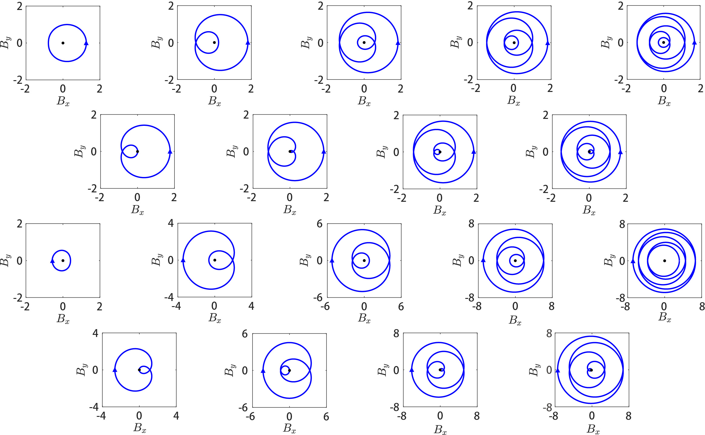
Figure 2: Curve of Bloch vector in the $B_{x}$-$B_{y}$ plane, the black dot is the origin. The corresponding knot or link eigenstate graph is depicted in Fig. 1 of the main text.

B: Linking number

In the gapped phase, the eigenstates $\left|\psi_{k}^{\pm}\right\rangle$ are represented by two loops on a torus surface, forming a torus link [Supplemental Figure 3(a)]. $\mathbf{r}_{+}\left(k\right)$ (blue loop) and $\mathbf{r}_{-}\left(k^{\prime}\right)$ (red loop) represent the positive branch $\left|\psi_{k}^{+}\right\rangle$ and the negative branch $\left|\psi_{k^{\prime}}^{-}\right\rangle$, respectively. We construct a vector field

$$\mathbf{h}\left(k,k^{\prime}\right)=\mathbf{r}_{+}\left(k\right)-\mathbf{r}_{-}\left(k^{\prime}\right),$$ (11)

where $\mathbf{r}_{+}\left(k\right)$ and $\mathbf{r}_{-}\left(k^{\prime}\right)$ in the cylindrical coordinate [Supplemental Figure 3(b)] are expressed as

$$\mathbf{r}_{+}\left(k\right) = 0\bm{\hat{\theta}}+r\sin\varphi_{+}\left(k\right)\mathbf{\hat{z}}+\left[R+r\cos\varphi_{+}\left(k\right)\right]\mathbf{\hat{r}},$$

$$\mathbf{r}_{-}\left(k^{\prime}\right) = 0\bm{\hat{\theta}}^{\prime}+r\sin\varphi_{-}\left(k^{\prime}\right)\mathbf{\hat{z}}^{\prime}+\left[R+r\cos\varphi_{-}\left(k^{\prime}\right)\right]\mathbf{\hat{r}}^{\prime}.$$ (12)

On the torus, $R$ (in red) is the distance from the center of the tube to the center of the torus, and $r$ (in purple) is the radius of the tube. Two cylindrical coordinates are related as follows

$$\mathbf{\hat{z}}^{\prime}=\mathbf{\hat{z},\hat{r}}^{\prime}=\cos\left(k^{\prime}-k\right)\mathbf{\hat{r}}+\sin\left(k^{\prime}-k\right)\bm{\hat{\theta}}.$$ (13)

Besides, we have $\varphi_{-}\left(k\right)=\varphi_{+}\left(k\right)+\pi$ and $\varphi_{-}\left(k^{\prime}\right)=\varphi_{+}\left(k^{\prime}\right)+\pi.$ Based on these relations, we have

$$\mathbf{h}\left(k,k^{\prime}\right)=h_{\theta}\bm{\hat{\theta}}+h_{z}\mathbf{\hat{z}}+h_{r}\mathbf{\hat{r}},$$ (14)

where

$$h_{\theta} = \left[R-r\cos\varphi_{+}\left(k^{\prime}\right)\right]\sin\left(k-k^{\prime}\right),$$

$$h_{z} = r\sin\varphi_{+}\left(k\right)+r\sin\varphi_{+}\left(k^{\prime}\right),$$ (15)

$$h_{r} = R+r\cos\varphi_{+}\left(k\right)-\left[R-r\cos\varphi_{+}\left(k^{\prime}\right)\right]\cos\left(k-k^{\prime}\right).$$

Each point $\left(k,k^{\prime}\right)$ is mapped to a three-dimensional vector $\mathbf{h}$. Since $k$ and $k^{\prime}$ are periodic parameters, the endpoint of vector $\mathbf{h}$ draws a deformed torus surface in the $\left(\bm{\theta},\mathbf{z},\mathbf{r}\right)$ space.

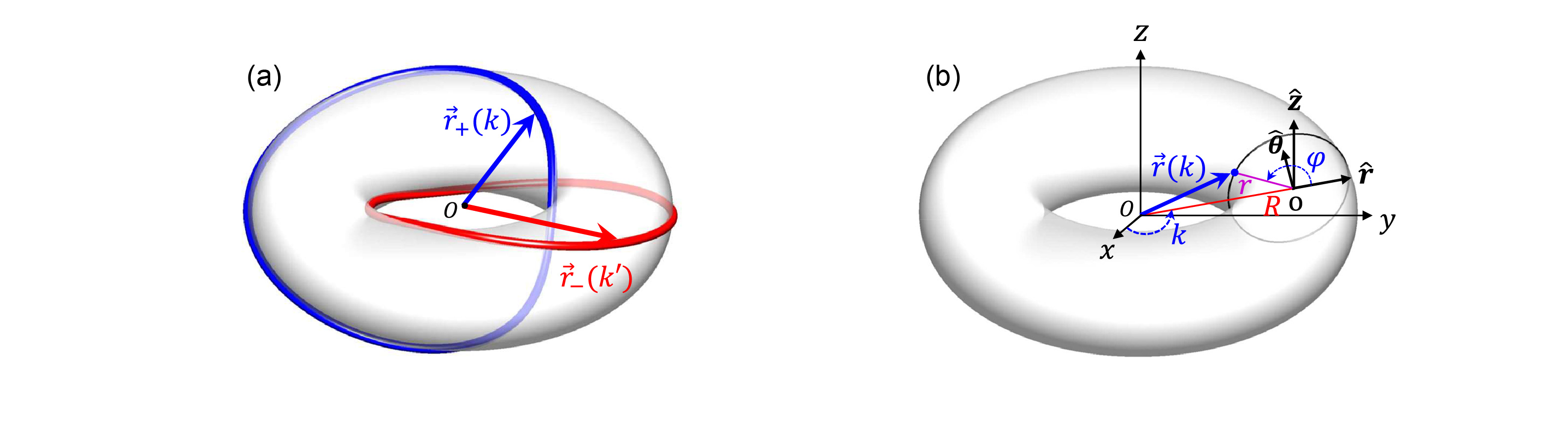
Figure 3: (a) A two-component Hopf link lies on the torus surface, each component is a closed loop of the eigenstate $\left|\psi_{k}^{\pm}\right\rangle$. (b) The cylindrical coordinate for the torus.

After introducing the vector field $\mathbf{h}$, we note that the linking number of two curves $\mathbf{r}_{+}\left(k\right)$ and $\mathbf{r}_{-}\left(k^{\prime}\right)$ in Eq. (8) of the main text can be expressed in the form of

$$L=\frac{1}{4\pi}\oint\nolimits_{k}\oint\nolimits_{k^{\prime}}\frac{\mathbf{h}}{\left|\mathbf{h}\right|^{3}}\cdot(\frac{\partial\mathbf{h}}{\partial k}\mathrm{d}k\times\frac{\partial\mathbf{h}}{\partial k^{\prime}}\mathrm{d}k^{\prime}).$$ (16)

Mathematically, the above expression of linking number is equal to the solid angle extended by the deformed torus surface dividing by $4\pi$ Asboth and the solid angle can be considered as twice the plane angle of the curve in the cross section of the deformed torus surface, whereas the cross section must contain the origin $\left(0,0,0\right)$ in the $\left(\bm{\theta},\mathbf{z},\mathbf{r}\right)$ space.

To get the cross section containing the origin, we set $h_{\theta}=0$. The $h_{\theta}=0$ plane cuts off the deformed torus surface to a curve in the $\left(\mathbf{z,r}\right)$ plane. By setting $h_{\theta}=0,$ we have $k^{\prime}=k$ and $\mathbf{h}$ is reduced to

$$\mathbf{h}=h_{z}\mathbf{\hat{z}}+h_{r}\mathbf{\hat{r}}=2r\sin\varphi_{+}\left(k\right)\mathbf{\hat{z}+}2r\cos\varphi_{+}\left(k\right)\mathbf{\hat{r}},$$ (17)

which indicates a closed circle $\Gamma$ centered at $\left(0,0\right)$ in the $\left(\mathbf{z,r}\right)$ plane and the linking number defined by the vector field $\mathbf{h}$ is given by

$$L=\frac{1}{2\pi}\oint_{\Gamma}\frac{1}{4r^{2}}\mathbf{(}h_{z}\nabla h_{r}-h_{r}\nabla h_{z})=-\frac{1}{2\pi}\int_{0}^{2\pi}\nabla_{k}\varphi_{+}\left(k\right)\mathrm{d}k.$$ (18)

Furthermore, from the definition $\varphi_{+}\left(k\right)=\arctan\left(-B_{y}/B_{x}\right)$, the linking number Eq. (18) can be expressed as

$$L=\frac{1}{2\pi}\oint_{C}\frac{1}{B^{2}}\mathbf{(}B_{x}\nabla B_{y}-B_{y}\nabla B_{x})=w.$$ (19)

The linking number $L$ is equivalent to the winding number $w$ defined in Eq. (6) of the main text.

References

- (1) C. C. Adams, The Knot Book (Freeman, New York, 1994).
- (2) J. W. Alexander and G. B. Briggs, On Types of Knotted Curves, Ann. Math. 28, 562 (1926).
- (3) S. A. Wasserman, J. M. Dungan, and N. R. Cozzarelli, Discovery of a Predicted DNA Knot Substantiates a Model for Site-Specific Recombination, Science 229, 171 (1985).
- (4) R. S. Forgan, J.-P. Sauvage, and J. F. Stoddart, Chemical Topology: Complex Molecular Knots, Links, and Entanglements, Chem. Rev. 111, 5434 (2011).
- (5) F. Wilczek and A. Zee, Linking Numbers, Spin, and Statistics of Solitons, Phys. Rev. Lett. 51, 2250 (1983).
- (6) C. Rovelli and L. Smolin, Knot Theory and Quantum Gravity, Phys. Rev. Lett. 61, 1155 (1988).
- (7) C. N. Yang and M. L. Ge, Braid Group, Knot Theory, and Statistical Mechanics (World Scientific, Singapore, 1989).
- (8) F. Y. Wu, Knot theory and statistical mechanics, Rev. Mod. Phys. 64, 1099 (1992).
- (9) M. Atiyah, Quantum physics and the topology of knots, Rev. Mod. Phys. 67, 977, (1995).
- (10) V. Katritch, J. Bednar, D. Michoud, R. G. Scharein, J. Dubochet, and A. Stasiak, Geometry and physics of knots, Nature 384, 142 (1996).
- (11) L. Faddeev and A. J. Niemi, Stable knot-like structures in classical field theory, Nature 387, 58 (1997).
- (12) L. H Kauffman, The mathematics and physics of knots, Rep. Prog. Phys. 68, 2829 (2005).
- (13) D. Kleckner and W. T. M. Irvine, Creation and dynamics of knotted vortices, Nat. Phys. 9, 253 (2013).
- (14) D. Kleckner, L. H. Kauffman, and W. T. M. Irvine, How superfluid vortex knots untie. Nat. Phys. 12, 650 (2016).
- (15) J. Leach, M. R. Dennis, J. Courtial, and M. J. Padgett, Knotted threads of darkness, Nature 432, 165 (2004).
- (16) M. R. Dennis, R. P. King, B. Jack, K. O’Holleran, and M. J. Padgett, Isolated optical vortex knots, Nat. Phys. 6, 118 (2010).
- (17) A. J. Taylor and M. R. Dennis, Vortex knots in tangled quantum eigenfunctions, Nat. Commun. 7, 12346 (2016).
- (18) D. S. Hall, M. W. Ray, K. Tiurev, E. Ruokokoski, A. H. Gheorghe and M. Möttönen, Tying quantum knots, Nat. Phys. 12, 478 (2016).
- (19) X.-Q. Sun, B. Lian, and S.-C. Zhang, Double Helix Nodal Line Superconductor, Phys. Rev. Lett. 119, 147001 (2017).
- (20) W. Chen, H.-Z. Lu, and J.-M. Hou, Topological semimetals with a double-helix nodal link, Phys. Rev. B 96, 041102(R) (2017).
- (21) M. Ezawa, Topological semimetals carrying arbitrary Hopf numbers: Fermi surface topologies of a Hopf link, Solomon’s knot, trefoil knot, and other linked nodal varieties, Phys. Rev. B 96, 041202(R) (2017).
- (22) R. Bi, Z. Yan, L. Lu, and Z. Wang, Nodal-knot semimetals, Phys. Rev. B 96, 201305(R) (2017).
- (23) Z. Yan, R. Bi, H. Shen, L. Lu, S.-C. Zhang, and Z. Wang, Nodal-link semimetals, Phys. Rev. B 96, 041103(R) (2017).
- (24) P.-Y. Chang and C.-H. Yee, Weyl-link semimetals, Phys. Rev. B 96, 081114(R) (2017).
- (25) P. J. Ackerman and I. I. Smalyukh, Diversity of Knot Solitons in Liquid CrystalsManifested by Linking of Preimages in Torons and Hopfions, Phys. Rev. X 7, 011006 (2017).
- (26) D.-L. Deng, S.-T. Wang, C. Shen, and L.-M. Duan, Phys. Rev. B 88, 201105(R) (2013).
- (27) D.-L. Deng, S.-T.Wang, K. Sun, and L.-M. Duan, Probe knots and Hopf insulators with ultracold atoms, arXiv:1612.01518.
- (28) Q. Yan, R. Liu, Z. Yan, B. Liu, H. Chen, Z. Wang, and L. Lu, Experimental discovery of nodal chains, Nat. Phys. 14, 461 (2018).
- (29) Z. Yang, C.-K. Chiu, C. Fang, and J. Hu, Evolution of nodal lines and knot transitions in topological semimetals, arXiv:1905.00210.
- (30) Z. Yang and J. Hu, Non-Hermitian Hopf-link exceptional line semimetals, Phys. Rev. B 99, 081102(R) (2019).
- (31) J. Carlström and E. J. Bergholtz, Exceptional links and twisted Fermi ribbons in non-Hermitian systems, Phys. Rev. A 98, 042114 (2018).
- (32) J. Carlström, M Strälhammar, J. C. Budich, and E. J. Bergholtz, Knotted non-Hermitian metals, Phys. Rev. B 99, 161115(R) (2019).
- (33) C. H. Lee, G. Li, Y. Liu, T. Tai, R. Thomale, and X. Zhang, Tidal surface states as fingerprints of non-Hermitian nodal knot metals, arXiv:1812.02011.
- (34) R. P. Feynman, Space-Time Appxoach to Quantum Electrodynamics, Phys. Rev. 76, 769 (1949).
- (35) G. Zhang, C. Li, and Z. Song, Majorana charges, winding numbers and Chern numbers in quantum Ising models, Sci. Rep. 7, 8176 (2017).
- (36) M. Suzuki, Relationship among Exactly Soluble Models of Critical Phenomena. I: 2D Ising Model, Dimer Problem and the Generalized XY-Model, Prog. Theor. Phys. 46, 1337 (1971).
- (37) S. Sachdev, Quantum Phase Transitions (Cambridge University Press, Cambridge, 1999).
- (38) A. Y. Kitaev, Unpaired Majorana fermions in quantum wires, Phys. Usp. 44, 131 (2001).
- (39) Y. Niu, S. B. Chung, C.-H. Hsu, I. Mandal, S. Raghu, and S. Chakravarty, Majorana zero modes in a quantum Ising chain with longer-ranged interactions, Phys. Rev. B 85, 035110 (2012).
- (40) Supplementary Material provides more details on the Bloch vector, winding number, and linking number.
- (41) X. M. Yang, P. Wang, L. Jin, and Z. Song, Visualizing topology of real-energy gapless phase arising from exceptional point, arXiv: 1905.07109.
- (42) J. W. Alexander, Topological invariants of knots and links, Trans. Am. Math. Soc. 20, 275 (1923).
- (43) J. K. Asbóth, L. Oroszlány, and A. Pályi, A Short Course on Topological Insulators: Band-structure topology and edge states in one and two dimensions (Springer, 2016).
- (44) Y. X. Zhao and A. P. Schnyder, Nonsymmorphic symmetry-required band crossings in topological semimetals, Phys. Rev. B 94, 195109 (2016).