Abstract

We study two randomized algorithms for generalized linear bandits. The first, $\tt GLM\mathchar 45\relax TSL$, samples a generalized linear model (GLM) from the Laplace approximation to the posterior distribution. The second, $\tt GLM\mathchar 45\relax FPL$, fits a GLM to a randomly perturbed history of past rewards. We analyze both algorithms and derive $\tilde{O}(d\sqrt{n\log K})$ upper bounds on their $n$-round regret, where $d$ is the number of features and $K$ is the number of arms. The former improves on prior work while the latter is the first for Gaussian noise perturbations in non-linear models. We empirically evaluate both $\tt GLM\mathchar 45\relax TSL$ and $\tt GLM\mathchar 45\relax FPL$ in logistic bandits, and apply $\tt GLM\mathchar 45\relax FPL$ to neural network bandits. Our work showcases the role of randomization, beyond posterior sampling, in exploration.

1 Introduction

A multi-armed bandit (Lai and Robbins, 1985; Auer et al., 2002; Lattimore and Szepesvari, 2019) is an online learning problem where actions of the learning agent are represented by arms. The arms can be treatments in a clinical trial or ads on a website. After an arm is pulled, the agent receives a stochastic reward. The agent aims to maximize its expected cumulative reward. Since the agent does not know the mean rewards of the arms in advance, it faces the exploration-exploitation dilemma: explore, and learn more about the reward distributions of the arms; or exploit, and pull the arm with the highest estimated reward thus far.

A generalized linear bandit (Filippi et al., 2010; Zhang et al., 2016; Li et al., 2017; Jun et al., 2017) is a variant of the multi-armed bandit where the expected rewards of arms are modeled using a generalized linear model (GLM) (McCullagh and Nelder, 1989). Specifically, the expected reward is a known function $\mu$, such as a sigmoid, of the dot product of a known feature vector and an unknown parameter vector. In the earlier clinical example, the feature and parameter vectors could be treatment indicators and effects of individual treatments, respectively.

Most existing algorithms for generalized linear bandits are based on upper confidence bounds (UCBs). Motivated by the superior performance of randomized GLM algorithms (Chapelle and Li, 2012; Russo et al., 2018), we study two randomized algorithms for this class of problems, $\tt GLM\mathchar 45\relax TSL$ and $\tt GLM\mathchar 45\relax FPL$. $\tt GLM\mathchar 45\relax TSL$ samples a GLM from the Laplace approximation to the posterior distribution. $\tt GLM\mathchar 45\relax FPL$ fits a GLM to a randomly perturbed history of past rewards.

We analyze $\tt GLM\mathchar 45\relax TSL$ and $\tt GLM\mathchar 45\relax FPL$, and prove that their $n$-round regret is $\tilde{O}(d\sqrt{n\log K})$, where $d$ is the number of features and $K$ is the number of arms. The regret bound of $\tt GLM\mathchar 45\relax TSL$ improves on the best prior regret bound (Abeille and Lazaric, 2017) by a multiplicative factor of $\sqrt{d/\log K}$ in the finite arm setting and matches it in the infinite arm setting. The regret bound of $\tt GLM\mathchar 45\relax FPL$ is the first for Gaussian noise perturbations in non-linear models, although we derive it under an additional assumption on arm features.

We also evaluate $\tt GLM\mathchar 45\relax TSL$ and $\tt GLM\mathchar 45\relax FPL$ empirically. Both have a state-of-the-art performance in logistic bandits, the most important practical use case of GLM bandits. Just as importantly, the perturbation scheme in $\tt GLM\mathchar 45\relax FPL$ generalizes straightforwardly to complex reward models, such as a neural network. To demonstrate this, we apply $\tt GLM\mathchar 45\relax FPL$ to high-dimensional classification problems and show that it can learn complex neural network mappings from features to rewards. The simplicity of $\tt GLM\mathchar 45\relax FPL$ suggests that it may find broad application in the future.

2 Setting

Algorithm 1 General randomized exploration in generalized linear bandits.

1:Inputs: Number of exploration rounds $\tau$

2:

3:for $t=1,\dots,n$ do

4:     if $t>\tau$ then

5:         $\tilde{\theta}_{t}\leftarrow$ Randomized MLE on $\left\{(X_{\ell},Y_{\ell})\right\}_{\ell=1}^{t-1}$

6:         $I_{t}\leftarrow\operatorname*{arg\,max\,}_{i\in[K]}x_{i}^{\top}\tilde{\theta}_{t}$

7:     else

8:         Choose $I_{t}$ based on $\left\{X_{\ell}\right\}_{\ell=1}^{t-1}$      

9:     Pull arm $I_{t}$ and get reward $Y_{I_{t},t}$

10:     $X_{t}\leftarrow x_{I_{t}},\ Y_{t}\leftarrow Y_{I_{t},t}$

We adopt the following notation. The set $\left\{1,\dots,n\right\}$ is denoted by $[n]$. All vectors are column vectors. For any positive semi-definite (PSD) matrix $M$, $\lambda_{\min}(M)\geq 0$ is the minimum eigenvalue of $M$. For any $n\times n$ PSD matrices $M_{1}$ and $M_{2}$, $M_{1}\preceq M_{2}$ if and only if $x^{\top}M_{1}x\leq x^{\top}M_{2}x$ for all $x\in\mathbb{R}^{d}$. We let $\|x\|_{M}=\sqrt{x^{\top}Mx}$ and $\mathrm{Ber}(p)$ be the Bernoulli distribution with mean $p$. The indicator that event $E$ occurs is $\mathds{1}\!\left\{E\right\}$. We use $\tilde{O}$ for the big-O notation up to logarithmic factors in horizon $n$.

A generalized linear model (GLM) is a probabilistic model where observation $Y$ given feature vector $x\in\mathbb{R}^{d}$ has an exponential-family distribution with mean $\mu(x^{\top}\theta)$, where $\mu$ is the mean function and $\theta\in\mathbb{R}^{d}$ are model parameters (McCullagh and Nelder, 1989). Let $\mathcal{D}=\left\{(x_{\ell},y_{\ell})\right\}_{\ell=1}^{n}$ be a set of $n$ observations, where $x_{\ell}\in\mathbb{R}^{d}$ and $y_{\ell}\in\mathbb{R}$. The negative log likelihood of $\mathcal{D}$ under model parameters $\theta$ is

$$L(\mathcal{D};\theta)=\sum_{\ell=1}^{\left|\mathcal{D}\right|}b(x_{\ell}^{\top}\theta)-y_{\ell}x_{\ell}^{\top}\theta-c(y_{\ell})\,,$$

where $c$ is a real function, and $b$ is twice continuously differentiable and its derivative is the mean function, $\dot{b}=\mu$. The gradient and Hessian of $L(\mathcal{D};\theta)$ with respect to $\theta$ are

$$\nabla L(\mathcal{D};\theta) =\sum_{\ell=1}^{\left|\mathcal{D}\right|}(\mu(x_{\ell}^{\top}\theta)-y_{\ell})x_{\ell}\,,$$ (1)

$$\nabla^{2}L(\mathcal{D};\theta) =\sum_{\ell=1}^{\left|\mathcal{D}\right|}\dot{\mu}(x_{\ell}^{\top}\theta)x_{\ell}x_{\ell}^{\top}\,,$$ (2)

where $\dot{\mu}$ denotes the derivative of $\mu$. The mean function $\mu$ is increasing and therefore its derivative $\dot{\mu}$ is positive. The maximum likelihood estimate (MLE) of model parameters is a vector $\theta\in\mathbb{R}^{d}$ such that $\nabla L(\mathcal{D};\theta)=\mathbf{0}$.

A stochastic GLM bandit (Filippi et al., 2010) is an online learning problem where the rewards of arms are generated by some underlying GLM. Let $K$ be the number of arms, $x_{i}\in\mathbb{R}^{d}$ be the feature vector of arm $i\in[K]$, and $\theta_{\ast}\in\mathbb{R}^{d}$ be an unknown parameter vector. The reward of arm $i$ in round $t\in[n]$, $Y_{i,t}$, is drawn i.i.d. from a distribution with mean $\mu_{i}=\mu(x_{i}^{\top}\theta_{\ast})$. We assume that $\eta_{i,t}=Y_{i,t}-\mu_{i}$ is $\sigma^{2}$-sub-Gaussian, that is

$$\mathbb{E}\left[\exp[\lambda\eta_{i,t}]\right]\leq\exp[\lambda^{2}\sigma^{2}/2]$$

holds for all arms $i$, rounds $t$, and $\lambda\geq 0$. In round $t$, the agent pulls arm $I_{t}\in[K]$ and observes its reward $Y_{I_{t},t}$. The goal of the agent is to maximize its expected cumulative reward in $n$ rounds. To simplify notation, we denote the feature vector of arm $I_{t}$ by $X_{t}=x_{I_{t}}$ and its stochastic reward by $Y_{t}=Y_{I_{t},t}$.

Without loss of generality, we assume that arm $1$ is the unique optimal arm, that is $\mu_{1}>\max_{i>1}\mu_{i}$. Let $\Delta_{i}=\mu_{1}-\mu_{i}$ be the suboptimality gap of arm $i$. Maximization of the expected cumulative reward over $n$ rounds is equivalent to minimizing the expected $n$-round regret, which is defined as

$$R(n)=\sum_{i=2}^{K}\Delta_{i}\mathbb{E}\left[\sum_{t=1}^{n}\mathds{1}\!\left\{I_{t}=i\right\}\right]\,.$$ (3)

3 Algorithms

Our GLM bandit algorithms follow the template in Algorithm 1. They explore initially in $\tau$ rounds, so that the estimated parameters in subsequent rounds have good properties. The exploration strategy is detailed in Section 4.5. After the initial exploration, they act greedily with respect to randomized parameter vectors $\tilde{\theta}_{t}$. Specifically, they pull arm $I_{t}=\operatorname*{arg\,max\,}_{i\in[K]}x_{i}^{\top}\tilde{\theta}_{t}$ in round $t$. If this maximum is not unique, any tie breaking can be used.

3.1 Algorithm $\tt GLM\mathchar 45\relax TSL$

We study two algorithms. The first algorithm, $\tt GLM\mathchar 45\relax TSL$, is a variant of Thompson sampling (Thompson, 1933) where the posterior of $\theta_{\ast}$ is approximated by its Laplace approximation. The randomized parameter vector is sampled from the Laplace approximation

$$\tilde{\theta}_{t}\sim\mathcal{N}(\bar{\theta}_{t},a^{2}H_{t}^{-1})\,,$$ (4)

where

$$\begin{split}\bar{\theta}_{t}&=\operatorname*{arg\,min\,}_{\theta\in\mathbb{R}^{d}}L(\left\{(X_{\ell},Y_{\ell})\right\}_{\ell=1}^{t-1};\theta)\,,\\ H_{t}&=\sum_{\ell=1}^{t-1}\dot{\mu}(X_{\ell}^{\top}\bar{\theta}_{t})X_{\ell}X_{\ell}^{\top}\,,\end{split}$$ (5)

and $a>0$ is a tunable parameter. Chapelle and Li (2012) and Russo et al. (2018) evaluated $\tt GLM\mathchar 45\relax TSL$ empirically. In addition, Abeille and Lazaric (2017) proved that $\tt GLM\mathchar 45\relax TSL$ has $\tilde{O}(d^{\frac{3}{2}}\sqrt{n})$ regret in the infinite arm setting. We prove that $\tt GLM\mathchar 45\relax TSL$ has $\tilde{O}(d\sqrt{n\log K})$ regret when the number of arms is $K$.

3.2 Algorithm $\tt GLM\mathchar 45\relax FPL$

We also propose a follow-the-perturbed-leader (FPL) algorithm, $\tt GLM\mathchar 45\relax FPL$. In $\tt GLM\mathchar 45\relax FPL$, the randomized parameter vector is the MLE from past $t-1$ rewards perturbed with Gaussian noise,

$$\tilde{\theta}_{t}=\operatorname*{arg\,min\,}_{\theta\in\mathbb{R}^{d}}L(\left\{(X_{\ell},Y_{\ell}+Z_{\ell})\right\}_{\ell=1}^{t-1};\theta)\,,$$ (6)

where $Z_{\ell}\sim\mathcal{N}(0,a^{2})$ are normal random variables that are resampled in each round, independently of each other and the history, and $a>0$ is a tunable parameter. Surprisingly, this perturbation does not change the parameter estimation problem. In particular, it only shifts the gradient of the log likelihood in (1) by $Z_{\ell}X_{\ell}$ and the Hessian in (2) remains positive semi-definite. In this work, we show that $\tt GLM\mathchar 45\relax FPL$ has $\tilde{O}(d\sqrt{n\log K})$ regret when the number of arms is $K$, under an additional assumption on arm features.

The design of $\tt GLM\mathchar 45\relax FPL$ is motivated by the equivalence of posterior sampling and perturbations by Gaussian noise in linear models (Lu and Van Roy, 2017), when the prior of $\theta_{\ast}$ and rewards are Gaussian. In GLMs, these two are not equivalent. Thus $\tt GLM\mathchar 45\relax TSL$ and $\tt GLM\mathchar 45\relax FPL$ are different algorithms. $\tt GLM\mathchar 45\relax FPL$ can be also viewed as an instance of randomized least-squares value iteration (Osband et al., 2016) applied to bandits. The specific instance in this work, additive Gaussian noise in a GLM, is novel. Finally, we note that the perturbation in (6) can be directly applied to more complex models, such as neural networks (Section 5). This is arguably its most attractive property.

3.3 Computationally-Efficient Implementations

The MLEs in (4) and (6) can be computed by iteratively reweighted least squares (IRLS) (Wolke and Schwetlick, 1988), which uses Newton’s method. Roughly speaking, each step of IRLS multiplies the inverse of (2) and (1). If (2) and (1) can be expressed independently of round $t$, the computational cost of an IRLS step does not increase with $t$. This is viable for any set of feature vectors $\mathcal{X}$ using

$$\textstyle\sum_{x\in\mathcal{X}}(N_{x}\mu(x^{T}\theta)-Y_{x})x\,,\quad\sum_{x\in\mathcal{X}}N_{x}\dot{\mu}(x^{T}\theta)xx^{T}\,,$$

where $N_{x}$ is the number of times that $x$ appears in history $\mathcal{D}$, and $Y_{x}$ is the sum of its rewards. Both $N_{x}$ and $Y_{x}$ can be updated incrementally. Finally, adding $\mathcal{N}(0,a^{2})$ noise to each reward in (6) is equivalent to adding $\mathcal{N}(0,N_{x}a^{2})$ noise to each $Y_{x}$ above.

The pulled arm in line 6 of Algorithm 1 can be computed efficiently even when the arm space is infinite, such as an intersection of half spaces. This is true of prior GLM bandit algorithms (Section 6). The MLE in line 5 cannot be computed efficiently in general, independently of round $t$, as in all prior algorithms except that of Jun et al. (2017). We study one approximation empirically in Section 5.2.

4 Analysis

Our analysis is organized as follows. In Section 4.1, we review technical challenges that arise in analyzing GLM bandits and their solutions. In Section 4.2, we outline our analysis. In Sections 4.3 and 4.4, we prove regret bounds for $\tt GLM\mathchar 45\relax TSL$ and $\tt GLM\mathchar 45\relax FPL$. We discuss them in Section 4.5.

4.1 Technical Challenges

One challenge in analyzing GLMs is that they do not have closed-form solutions. Nevertheless, their solutions can be expressed using the gradient and Hessian of the log likelihood (Section 2). This is the key idea in the analyses of GLM bandits (Filippi et al., 2010; Li et al., 2017) and we present it below.

Lemma 1.

Let $\mathcal{D}_{1}=\left\{(x_{\ell},y_{\ell,1})\right\}_{\ell=1}^{n}$ be a set of $n$ observations and $\mathcal{D}_{2}=\left\{(x_{\ell},y_{\ell,2})\right\}_{\ell=1}^{n}$ have the same features as $\mathcal{D}_{1}$. Let $\theta_{1}$ be the minimizer of $L(\mathcal{D}_{1};\theta)$ and $\theta_{2}$ be the minimizer of $L(\mathcal{D}_{2};\theta)$. Then

$$\sum_{\ell=1}^{n}(y_{\ell,2}-y_{\ell,1})x_{\ell}=\nabla^{2}L(\mathcal{D}_{1};\theta^{\prime})(\theta_{2}-\theta_{1})\,,$$

where $\theta^{\prime}=\alpha\theta_{1}+(1-\alpha)\theta_{2}$ for some $\alpha\in[0,1]$.

Proof.

By the definition of the gradient in (1),

$$\nabla L(\mathcal{D}_{1};\theta)-\nabla L(\mathcal{D}_{2};\theta)=\sum_{\ell=1}^{n}(y_{\ell,2}-y_{\ell,1})x_{\ell}$$

holds for any $\theta$. Moreover, from the definitions of $\theta_{1}$ and $\theta_{2}$, $\nabla L(\mathcal{D}_{1};\theta_{1})=\nabla L(\mathcal{D}_{2};\theta_{2})=\mathbf{0}$. Now we apply these identities and obtain

$$\sum_{\ell=1}^{n}(y_{\ell,2}-y_{\ell,1})x_{\ell} =\nabla L(\mathcal{D}_{1};\theta_{2})-\nabla L(\mathcal{D}_{2};\theta_{2})$$

$$=\nabla L(\mathcal{D}_{1};\theta_{2})-\nabla L(\mathcal{D}_{1};\theta_{1})$$

$$=\nabla^{2}L(\mathcal{D}_{1};\theta^{\prime})(\theta_{2}-\theta_{1})\,.$$

where $\theta^{\prime}$ is defined in the claim. ∎

Another challenge is $\dot{\mu}(x_{\ell}^{\top}\theta)$ in (2). To apply ideas from linear bandit analyses, it must be eliminated. We do so as follows. Let $G=\sum_{\ell=1}^{\left|\mathcal{D}\right|}x_{\ell}x_{\ell}^{\top}$ be an unweighted Hessian with the same features as (2). Let $c_{\min}\leq\dot{\mu}(x_{\ell}^{\top}\theta)\leq c_{\max}$ for some $c_{\min}$ and $c_{\max}$, and for all $\ell\in[\left|\mathcal{D}\right|]$. Then from the definition of (2), $c_{\min}G\preceq\nabla^{2}L(\mathcal{D};\theta)\preceq c_{\max}G$ and $c_{\min}^{-1}G^{-1}\succeq(\nabla^{2}L(\mathcal{D};\theta))^{-1}\succeq c_{\max}^{-1}G^{-1}$. Because of this, the derivatives of $\mu$ must be controlled.

To control the derivatives of $\mu$ at $\bar{\theta}_{t}$ and $\tilde{\theta}_{t}$ (Section 3), we initially explore so that $\bar{\theta}_{t}$ and $\tilde{\theta}_{t}$ are in the unit ball centered at $\theta_{\ast}$ with a high probability. This gives rise to

$$\textstyle\dot{\mu}_{\min}=\min_{\|x\|_{2}\leq 1,\,\|\theta-\theta_{\ast}\|_{2}\leq 1}\dot{\mu}(x^{\top}\theta)$$

in our regret bounds, the minimum derivative of $\mu$ in the unit ball centered at $\theta_{\ast}$. This trick (Li et al., 2017) requires that $\|x_{i}\|_{2}\leq 1$ for all arms $i$, and we assume this in our analysis. We define the maximum derivative of $\mu$ as

$$\textstyle\dot{\mu}_{\max}=\max_{\|x\|_{2}\leq 1,\,\theta\in\mathbb{R}^{d}}\dot{\mu}(x^{\top}\theta)\,.$$

This factor is typically easy to control. In logistic regression, for instance, $\dot{\mu}_{\max}=1/4$.

4.2 Outline of Our Analyses

Let $\theta_{\ast}$ be the unknown parameter vector, $\bar{\theta}_{t}$ be its MLE in round $t$, and $\tilde{\theta}_{t}$ be the randomized MLE in round $t$. At a high level, we bound the regret under assumptions that $\bar{\theta}_{t}\to\theta_{\ast}$, $\tilde{\theta}_{t}\to\bar{\theta}_{t}$, and $\tilde{\theta}_{t}$ is optimistic. We show that the corresponding favorable conditions hold with a high probability and define the corresponding events below.

Let $\mathcal{F}_{t}=\sigma(I_{1},\dots,I_{t},Y_{1},\dots,Y_{t})$ be the $\sigma$-algebra generated by the pulled arms and their rewards by the end of round $t\in[n]$. We let $\mathcal{F}_{0}=\left\{\emptyset,\Omega\right\}$, where $\Omega$ is the sample space of the probability space that holds all random variables. Then $(\mathcal{F}_{t})_{t}$ is a filtration. Let

$$\mathbb{P}_{t}\left(\cdot\right)=\mathbb{P}\left(\cdot\,\middle|\,\mathcal{F}_{t-1}\right)\,,\quad\mathbb{E}_{t}\left[\cdot\right]=\mathbb{E}\left[\cdot\,\middle|\,\mathcal{F}_{t-1}\right]\,,$$

be the conditional probability and expectation, given the history at the beginning of round $t$, $\mathcal{F}_{t-1}$, respectively. Let $G_{t}=\sum_{\ell=1}^{t-1}X_{\ell}X_{\ell}^{\top}$ be the unweighted Hessian in round $t$ and $\Delta_{\max}=\max_{i\in[K]}\Delta_{i}$ be the maximum regret.

To argue that $\bar{\theta}_{t}\to\theta_{\ast}$, we define

$$E_{1,t}=\left\{\forall i\in[K]:\left|x_{i}^{\top}\bar{\theta}_{t}-x_{i}^{\top}\theta_{\ast}\right|\leq c_{1}\|x_{i}\|_{G_{t}^{-1}}\right\}\,,$$ (7)

the event that $x_{i}^{\top}\bar{\theta}_{t}$ and $x_{i}^{\top}\theta_{\ast}$ are close for all arms $i$ in round $t$, where $c_{1}>0$ is tuned later such that event $E_{1,t}$ is likely. Specifically, let $\bar{E}_{1,t}$ be the complement of $E_{1,t}$. Then we set $c_{1}$ such that $\mathbb{P}\left(\bar{E}_{1,t}\right)=O(1/n)$.

The upper bound on $\mathbb{P}\left(\bar{E}_{1,t}\right)$ is motivated by Lemma 3 in Li et al. (2017). We reprove the lemma since it contains a subtle error. In particular, the proof that $\|\bar{\theta}_{t}-\theta_{\ast}\|_{2}\leq 1$ holds with a high probability assumes that the agent does not act adaptively up to round $t$, which it clearly does for any $t>\tau$.

To argue that $\tilde{\theta}_{t}\to\bar{\theta}_{t}$, we define

$$E_{2,t}=\left\{\forall i\in[K]:\left|x_{i}^{\top}\tilde{\theta}_{t}-x_{i}^{\top}\bar{\theta}_{t}\right|\leq c_{2}\|x_{i}\|_{G_{t}^{-1}}\right\}\,,$$ (8)

the event that $x_{i}^{\top}\tilde{\theta}_{t}$ and $x_{i}^{\top}\bar{\theta}_{t}$ are close for all arms $i$ in round $t$, where $c_{2}>0$ is tuned later such that event $E_{2,t}$ is likely given any past. Specifically, let $\bar{E}_{2,t}$ be the complement of $E_{2,t}$. Then we set $c_{2}$ such that $\mathbb{P}_{t}\left(\bar{E}_{2,t}\right)=O(1/n)$. This part of the analysis relies on the properties of our perturbations and is novel.

Finally, to argue that $\tilde{\theta}_{t}$ is sufficiently optimistic given any past, we define event

$$E_{3,t}=\left\{x_{1}^{\top}\tilde{\theta}_{t}-x_{1}^{\top}\bar{\theta}_{t}>c_{1}\|x_{1}\|_{G_{t}^{-1}}\right\}.$$ (9)

To obtain $\mathbb{P}_{t}\left(E_{3,t}\right)=O(1)$, we set parameter $a$ in (4) and (6). This part of the analysis relies on the properties of our perturbations and is novel.

Our analysis is sufficiently general, so that it can be used to analyze different randomized algorithms. To show this, we use it to analyze both $\tt GLM\mathchar 45\relax TSL$ and $\tt GLM\mathchar 45\relax FPL$. The central part of the analysis is an upper bound on the expected per-round regret of any randomized algorithm whose perturbed solution in round $t$ is a function of its history. The corresponding lemma is stated below.

[]lemmaperroundregret Let $p_{2}\geq\mathbb{P}_{t}\left(\bar{E}_{2,t}\right)$, $p_{3}\leq\mathbb{P}_{t}\left(E_{3,t}\right)$, and $p_{3}>p_{2}$. Then on event $E_{1,t}$,

$$\mathbb{E}_{t}\left[\Delta_{I_{t}}\right]\leq{} \dot{\mu}_{\max}(c_{1}+c_{2})\left(1+\frac{2}{p_{3}-p_{2}}\right)\times{}$$

$$\mathbb{E}_{t}\left[\|x_{I_{t}}\|_{G_{t}^{-1}}\right]+\Delta_{\max}\,p_{2}\,.$$

The hardest part in the analyses of $\tt GLM\mathchar 45\relax TSL$ and $\tt GLM\mathchar 45\relax FPL$ is to bound $p_{2}$ and $p_{3}$ in Section 4.2.

4.3 Analysis of $\tt GLM\mathchar 45\relax TSL$

Now we are ready to analyze $\tt GLM\mathchar 45\relax TSL$ and $\tt GLM\mathchar 45\relax FPL$. The regret bound of $\tt GLM\mathchar 45\relax TSL$ is stated below.

[]theoremglmtslregretbound The $n$-round regret of $\tt GLM\mathchar 45\relax TSL$ is bounded as

$$R(n)\leq{} \dot{\mu}_{\max}(c_{1}+c_{2})\left(1+\frac{2}{0.15-1/n}\right)\times{}$$

$$\sqrt{2dn\log(2n/d)}+(\tau+3)\Delta_{\max}\,,$$

where

$$a =c_{1}\sqrt{\dot{\mu}_{\max}}\,,$$

$$c_{1} =\sigma\dot{\mu}_{\min}^{-1}\sqrt{d\log(n/d)+2\log n}\,,$$

$$c_{2} =c_{1}\sqrt{2\dot{\mu}_{\min}^{-1}\,\dot{\mu}_{\max}\log(Kn)}\,,$$

and the number of exploration rounds $\tau$ satisfies

$$\lambda_{\min}(G_{\tau})\geq\max\left\{\sigma^{2}\dot{\mu}_{\min}^{-2}(d\log(n/d)+2\log n),\,1\right\}\,.$$

Proof.

The claim is proved in Appendix A.

The proof has three key steps. First, we bound the probability of event $\bar{E}_{1,t}$ from above (Lemma 5 in Appendix B). Second, we choose parameter $a$ such that the probabilities of events $\bar{E}_{2,t}$ and $E_{3,t}$ are bounded for any history $\mathcal{F}_{t-1}$ (Lemma 2). Finally, we set the number of initial exploration rounds $\tau$ such that $\|\bar{\theta}_{t}-\theta_{\ast}\|_{2}\leq 1$ is likely in any round $t\geq\tau$ (Lemma 6 in Appendix B). ∎

The above regret bound is $\tilde{O}(d\sqrt{n\log K})$. We derive the key concentration and anti-concentration lemma below.

Lemma 2.

Let

$$a=c_{1}\sqrt{\dot{\mu}_{\max}}\,,\quad c_{2}=c_{1}\sqrt{2\dot{\mu}_{\min}^{-1}\,\dot{\mu}_{\max}\log(Kn)}\,.$$

Let $E=\left\{\|\bar{\theta}_{t}-\theta_{\ast}\|_{2}\leq 1\right\}$. Then $\mathbb{P}_{t}\left(\bar{E}_{2,t}\right)\leq 1/n$ holds on event $E$ and $\mathbb{P}_{t}\left(E_{3,t}\right)\geq 0.15$.

Proof.

By the design of $\tt GLM\mathchar 45\relax TSL$ in (4),

$$x^{\top}\tilde{\theta}_{t}-x^{\top}\bar{\theta}_{t}\sim\mathcal{N}(0,a^{2}\|x\|_{H_{t}^{-1}}^{2})$$

for any vector $x\in\mathbb{R}^{d}$, where matrix $H_{t}$ is defined in (5). Let $U=x^{\top}\tilde{\theta}_{t}-x^{\top}\bar{\theta}_{t}$. Because $U\sim\mathcal{N}(0,a^{2}\|x\|_{H_{t}^{-1}}^{2})$ is a normal random variable, we have that

$$\mathbb{P}_{t}\left(U\geq a\|x\|_{H_{t}^{-1}}\right) \geq 0.15\,,$$

$$\mathbb{P}_{t}\left(U\geq c\|x\|_{H_{t}^{-1}}\right) \leq\exp\left[-\frac{c^{2}}{2a^{2}}\right]\,,$$

for any $c>0$.

Now note that $H_{t}\preceq\dot{\mu}_{\max}G_{t}$. As a result,

$$0.15 \leq\mathbb{P}_{t}\left(U\geq a\|x\|_{H_{t}^{-1}}\right)$$

$$\leq\mathbb{P}_{t}\left(U\geq a\sqrt{\dot{\mu}_{\max}^{-1}}\|x\|_{G_{t}^{-1}}\right)\,.$$

For $a=c_{1}\sqrt{\dot{\mu}_{\max}}$ and $x=x_{1}$, we get that event $E_{3,t}$ in (9) occurs with probability at least $0.15$.

Moreover, $H_{t}\succeq\dot{\mu}_{\min}G_{t}$ on event $E$, which yields

$$\exp\left[-\frac{c^{2}}{2a^{2}}\right] \geq\mathbb{P}_{t}\left(U\geq c\|x\|_{H_{t}^{-1}}\right)$$

$$\geq\mathbb{P}_{t}\left(U\geq c\sqrt{\dot{\mu}_{\min}^{-1}}\|x\|_{G_{t}^{-1}}\right)\,.$$

For $c=a\sqrt{2\log(Kn)}$, $x=x_{i}$, and by the union bound over all $K$ arms, we get that event $\bar{E}_{2,t}$ in (8) occurs with probability at most $1/n$. ∎

4.4 Analysis of $\tt GLM\mathchar 45\relax FPL$

The regret bound of $\tt GLM\mathchar 45\relax FPL$ is stated below. The analysis assumes that all feature vectors $x_{i}$ have at most one non-zero entry. This assumption is discussed in Section 4.5.

[]theoremglmfplregretbound The $n$-round regret of $\tt GLM\mathchar 45\relax FPL$ is bounded as

$$R(n)\leq{} \dot{\mu}_{\max}(c_{1}+c_{2})\left(1+\frac{2}{0.15-2/n}\right)\times{}$$

$$\sqrt{2dn\log(2n/d)}+(\tau+4)\Delta_{\max}\,,$$

where

$$a =c_{1}\dot{\mu}_{\max}\,,$$

$$c_{1} =\sigma\dot{\mu}_{\min}^{-1}\sqrt{d\log(n/d)+2\log n}\,,$$

$$c_{2} =c_{1}\dot{\mu}_{\min}^{-1}\,\dot{\mu}_{\max}\sqrt{2\log(Kn)}\,,$$

and the number of exploration rounds $\tau$ satisfies

$$\lambda_{\min}(G_{\tau})\geq\max\{ 4\sigma^{2}\dot{\mu}_{\min}^{-2}(d\log(n/d)+2\log n),$$

$$8a^{2}\dot{\mu}_{\min}^{-2}\log n,\,1\}\,.$$

Proof.

The claim is proved in Appendix A.

The proof has three key steps. First, we bound the probability of event $\bar{E}_{1,t}$ from above (Lemma 5 in Appendix B). Second, we choose parameter $a$ such that the probabilities of events $\bar{E}_{2,t}$ and $E_{3,t}$ are bounded for any history $\mathcal{F}_{t-1}$ (Lemma 3). Finally, we set the number of initial exploration rounds $\tau$ such that $\|\bar{\theta}_{t}-\theta_{\ast}\|_{2}\leq 1/2$ is likely and $\|\tilde{\theta}_{t}-\theta_{\ast}\|_{2}\leq 1$ is conditionally likely given $\mathcal{F}_{t-1}$, in any round $t\geq\tau$ (Lemma 7 in Appendix B). ∎

The above regret bound is also $\tilde{O}(d\sqrt{n\log K})$. The key concentration and anti-concentration lemma follows.

Lemma 3.

Let

$$a=c_{1}\dot{\mu}_{\max}\,,\quad c_{2}=c_{1}\dot{\mu}_{\min}^{-1}\,\dot{\mu}_{\max}\sqrt{2\log(Kn)}\,.$$

Let $E=\left\{\|\bar{\theta}_{t}-\theta_{\ast}\|_{2}\leq 1/2\right\}$, $E^{\prime}=\{\|\tilde{\theta}_{t}-\theta_{\ast}\|_{2}\leq 1\}$, and $\mathbb{P}_{t}\left(\bar{E}^{\prime}\right)\leq 1/n$ on event $E$. Then $\mathbb{P}_{t}\left(\bar{E}_{2,t}\right)\leq 2/n$ on event $E$ and $\mathbb{P}_{t}\left(E_{3,t}\right)\geq 0.15$.

Proof.

Fix any history $\mathcal{F}_{t-1}$. By Lemma 1, where $\mathcal{D}_{1}=\left\{(X_{\ell},Y_{\ell})\right\}_{\ell=1}^{t-1}$ and $\mathcal{D}_{2}=\left\{(X_{\ell},Y_{\ell}+Z_{\ell})\right\}_{\ell=1}^{t-1}$, we get

$$\sum_{\ell=1}^{t-1}Z_{\ell}X_{\ell}=\tilde{H}_{t}(\tilde{\theta}_{t}-\bar{\theta}_{t})\,,$$

where $Z_{\ell}\in\mathcal{N}(0,a^{2})$ are i.i.d. normal random variables,

$$\tilde{H}_{t}=\sum_{\ell=1}^{t-1}\dot{\mu}(X_{\ell}^{\top}\theta^{\prime}_{t})X_{\ell}X_{\ell}^{\top}\,,$$

and $\theta^{\prime}_{t}=\alpha\bar{\theta}_{t}+(1-\alpha)\tilde{\theta}_{t}$ for some $\alpha\in[0,1]$. Fix any $x\in\mathbb{R}^{d}$ and let $U=x^{\top}G_{t}^{-1}\sum_{\ell=1}^{t-1}Z_{\ell}X_{\ell}$. Then

$$x^{\top}G_{t}^{-1}\tilde{H}_{t}(\tilde{\theta}_{t}-\bar{\theta}_{t})=U\sim\mathcal{N}(0,a^{2}\|x\|_{G_{t}^{-1}}^{2})\,.$$

Since $U$ is a normal random variable, we have that

$$\mathbb{P}_{t}\left(U\geq a\|x\|_{G_{t}^{-1}}\right) \geq 0.15\,,$$

$$\mathbb{P}_{t}\left(U\geq c\|x\|_{G_{t}^{-1}}\right) \leq\exp\left[-\frac{c^{2}}{2a^{2}}\right]\,,$$

for any $c>0$.

Since all feature vectors have at most one non-zero entry, $G_{t}^{-1}$ and $\tilde{H}_{t}$ are diagonal, as is $G_{t}^{-1}\tilde{H}_{t}$. By the definitions of $G_{t}$ and $\tilde{H}_{t}$, diagonal entries of $G_{t}^{-1}\tilde{H}_{t}$ are non-negative and at most $\dot{\mu}_{\max}$. Let $x$ have at most one non-zero entry. Then $x^{\top}(\tilde{\theta}_{t}-\bar{\theta}_{t})$ and $x^{\top}G_{t}^{-1}\tilde{H}_{t}(\tilde{\theta}_{t}-\bar{\theta}_{t})$ have the same sign, which we use to derive

$$0.15 \leq\mathbb{P}_{t}\left(U\geq a\|x\|_{G_{t}^{-1}}\right)$$

$$\leq\mathbb{P}_{t}\left(\dot{\mu}_{\max}\,x^{\top}(\tilde{\theta}_{t}-\bar{\theta}_{t})\geq a\|x\|_{G_{t}^{-1}}\right)$$

$$=\mathbb{P}_{t}\left(x^{\top}(\tilde{\theta}_{t}-\bar{\theta}_{t})\geq a\dot{\mu}_{\max}^{-1}\|x\|_{G_{t}^{-1}}\right)\,.$$

For $a=c_{1}\dot{\mu}_{\max}$ and $x=x_{1}$, we get that event $E_{3,t}$ in (9) occurs with probability at least $0.15$.

The diagonal entries of $G_{t}^{-1}\tilde{H}_{t}$ are non-negative, and also at least $\dot{\mu}_{\min}$ on events $E$ and $E^{\prime}$. So, on event $E$,

$$\exp\left[-\frac{c^{2}}{2a^{2}}\right] \geq\mathbb{P}_{t}\left(U\geq c\|x\|_{G_{t}^{-1}}\right)$$

$$\geq\mathbb{P}_{t}\left(U\geq c\|x\|_{G_{t}^{-1}},\,E^{\prime}\text{ occurs}\right)$$

$$\geq\mathbb{P}_{t}\left(\dot{\mu}_{\min}\,x^{\top}(\tilde{\theta}_{t}-\bar{\theta}_{t})\geq c\|x\|_{G_{t}^{-1}}\right)-\frac{1}{n}$$

$$=\mathbb{P}_{t}\left(x^{\top}(\tilde{\theta}_{t}-\bar{\theta}_{t})\geq c\dot{\mu}_{\min}^{-1}\|x\|_{G_{t}^{-1}}\right)-\frac{1}{n}\,.$$

For $c=a\sqrt{2\log(Kn)}$, $x=x_{i}$, and by the union bound over all $K$ arms, we get that event $\bar{E}_{2,t}$ in (8) occurs with probability at most $2/n$. ∎

4.5 Discussion

The regret of $\tt GLM\mathchar 45\relax TSL$ is $\tilde{O}(d\sqrt{n\log K})$ (Section 4.3). Up to the factor of $\sqrt{\log K}$, this matches the gap-free bounds of $\tt GLM\mathchar 45\relax UCB$ (Filippi et al., 2010) and $\tt UCB\mathchar 45\relax GLM$ (Li et al., 2017). As in Agrawal and Goyal (2013b), the key idea in our analysis is to achieve optimism by inflating the covariance matrix in $\tt GLM\mathchar 45\relax TSL$ by $a=O(\sqrt{d\log n})$. This setting is too conservative in practice. Thus, in Section 5, we also experiment with $a=O(1)$, which is known to work well in practice (Chapelle and Li, 2012; Russo et al., 2018).

The regret of $\tt GLM\mathchar 45\relax FPL$ is $\tilde{O}(d\sqrt{n\log K})$ (Section 4.4). Although the bound scales with $K$, $d$, and $n$ similarly to that in Section 4.3, it is worse in constant factors. For instance, $c_{2}$ is additionally multiplied by $\sqrt{\dot{\mu}_{\min}^{-1}\,\dot{\mu}_{\max}}$. The number of initial exploration rounds is also higher, since we need to guarantee that $\tilde{\theta}_{t}$ and $\theta_{\ast}$ are close with a high probability given any $\mathcal{F}_{t-1}$. As in $\tt GLM\mathchar 45\relax TSL$, the suggested value of $a=O(\sqrt{d\log n})$ is too conservative in practice. Thus, we also experiment with $a=O(1)$ in Section 5.

The regret bound of $\tt GLM\mathchar 45\relax FPL$ is proved under the assumption that feature vectors have at most one non-zero entry. We need this assumption for the following reason. We establish in Lemma 3 that

$$U=x^{\top}G_{t}^{-1}\tilde{H}_{t}(\tilde{\theta}_{t}-\bar{\theta}_{t})\sim\mathcal{N}(0,a^{2}\|x\|_{G_{t}^{-1}}^{2})\,.$$

Since $a\|x\|_{G_{t}^{-1}}$ is one standard deviation of $U$, event $U>a\|x\|_{G_{t}^{-1}}$ is likely. But we need event $U^{\prime}=x^{\top}(\tilde{\theta}_{t}-\bar{\theta}_{t})>a\|x\|_{G_{t}^{-1}}$ to be likely. If $G_{t}^{-1}$ and $\tilde{H}_{t}$ have different eigenvectors, $U$ and $U^{\prime}$ can have different signs, and it is hard to relate them due to potential rotations by $G_{t}^{-1}\tilde{H}_{t}$. Our assumption guarantees that the eigenvectors of $G_{t}^{-1}$ and $\tilde{H}_{t}$ are identical. We leave the elimination of this assumption for future work.

The initial exploration in $\tt GLM\mathchar 45\relax TSL$ and $\tt GLM\mathchar 45\relax FPL$ can be implemented as follows. Let $\left\{v_{i}\right\}_{i=1}^{d}\subseteq\left\{x_{i}\right\}_{i=1}^{K}$ be any basis in $\mathbb{R}^{d}$ and $M=\sum_{i=1}^{d}v_{i}^{\top}v_{i}$. Then, to satisfy assumptions $\lambda_{\min}(G_{\tau})\geq C$ in Sections 4.3 and 4.4, each arm in the basis is pulled $C\lambda_{\min}^{-1}(M)$ times.

5 Experiments

We conduct two sets of experiments. In Section 5.1, we assess the empirical regret of $\tt GLM\mathchar 45\relax TSL$ and $\tt GLM\mathchar 45\relax FPL$ in logistic bandits. Because of its simplicity and generality, the perturbation mechanism in $\tt GLM\mathchar 45\relax FPL$ can be easily applied to more complex models. We assess it on contextual bandit problems with neural networks in Section 5.2.

5.1 Logistic Bandit

The goal of this experiment is to show that our proposed algorithms perform well. We experiment with a logistic bandit, a GLM bandit where $\mu(v)=1/(1+\exp[-v])$ and $Y_{i,t}\sim\mathrm{Ber}(\mu(x_{i}^{\top}\theta_{\ast}))$. The number of arms is $K=100$. To avoid bias in choosing problem instances, we generate them randomly: the feature vector of arm $i$ is drawn uniformly at random from $[-1,1]^{d}$ and the parameter vector is $\theta_{\ast}\sim\mathcal{N}(\mathbf{0},3d^{-2}I_{d})$, where $I_{d}$ is a $d\times d$ identity matrix. By design, $\mathrm{var}\left[x_{i}^{\top}\theta_{\ast}\right]=1$, and so $x_{i}^{\top}\theta_{\ast}\in[-4,4]$ with a high probability. We vary the number of features $d$ from $5$ to $20$. The horizon is $n=50\,000$ rounds and our results are averaged over $100$ problem instances.

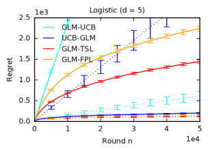
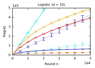
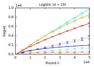
Figure 1: Evaluation of $\tt GLM\mathchar 45\relax TSL$ and $\tt GLM\mathchar 45\relax FPL$ in logistic bandits. The $n$-round regret is shown as a function of $n$. The solid and dotted lines represented theory-suggested and informal designs, respectively.

Our baselines are two UCB algorithms, $\tt GLM\mathchar 45\relax UCB$ (Filippi et al., 2010) and $\tt UCB\mathchar 45\relax GLM$ (Li et al., 2017). We experiment with two designs for each evaluated algorithm, theory (as analyzed) and informal (practical). For $\tt GLM\mathchar 45\relax TSL$, we use $a$ from Section 4.3 and $a=1$, for which (4) reduces to sampling from the Laplace approximation. For $\tt GLM\mathchar 45\relax FPL$, we use $a$ from Section 4.4 and $a=0.5$. We choose the latter since $a$ in Section 4.4 is half that in Section 4.3 in logistic models, since $\dot{\mu}_{\max}=0.25$. We also implement $\tt GLM\mathchar 45\relax UCB$ and $\tt UCB\mathchar 45\relax GLM$ with tighter confidence intervals, $0.5\|x\|_{G^{-1}}$, where $x$ is the feature vector of the arm, $G$ is the sample covariance matrix, and $0.5$ is the maximum standard deviation of rewards in logistic models. All algorithms pull $d$ linearly independent arms initially and $\dot{\mu}_{\min}$ is set to the most optimistic value of $0.25$.

Our results are shown in Figure 1. We observe that theory $\tt GLM\mathchar 45\relax TSL$ and $\tt GLM\mathchar 45\relax FPL$ outperform theory $\tt GLM\mathchar 45\relax UCB$, but not theory $\tt UCB\mathchar 45\relax GLM$. The latter is known from prior algorithm designs. In particular, when $\tt LinTS$ (Agrawal and Goyal, 2013b) is implemented as analyzed, it fails to outperform $\tt LinUCB$ (Abbasi-Yadkori et al., 2011); but it does outperform it when the theory-suggested posterior scaling is relaxed. This is indeed how $\tt LinTS$ is usually implemented. Informal $\tt GLM\mathchar 45\relax UCB$ and $\tt UCB\mathchar 45\relax GLM$ fail, and have linear regret in $n$. On the other hand, informal $\tt GLM\mathchar 45\relax TSL$ and $\tt GLM\mathchar 45\relax FPL$ have low regret, sublinear in $n$. We conclude that $\tt GLM\mathchar 45\relax TSL$ and $\tt GLM\mathchar 45\relax FPL$ have state-of-the-art performance in logistic bandits.

5.2 Deep Bandit

The second experiment is on contextual bandit problems, which are generated as follows. We fix a supervised learning dataset $\mathcal{D}$ and a target label $c$. The examples with label $c$ have random rewards $\mathrm{Ber}(0.75)$ while the other examples have random rewards $\mathrm{Ber}(0.25)$. In round $t$, the agent is presented $K=10$ random examples $x_{i,t}$ from $\mathcal{D}$, which are arms. The agent learns a single generalization model that maps feature vector $x_{i,t}$ to its expected reward. The goal of the agent is to learn a good mapping quickly. Since our generalization models are imperfect, our evaluation metric is the average per-round reward in $n$ rounds, which we define as $\sum_{t=1}^{n}Y_{t}/n$.

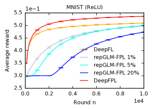
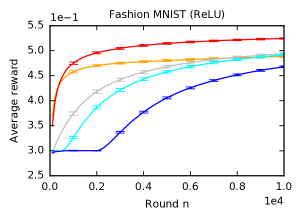
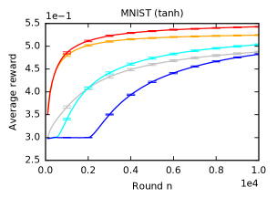
Figure 2: Evaluation of $\tt DeepFPL$ on contextual bandit problems in Section 5.2.

We experiment with two large-scale datasets: MNIST and Fashion MNIST. MNIST (Lecun et al., 1998) is a dataset of $60$ thousand $28\times 28$ gray-scale images of handwritten digits, from $0$ to $9$. Fashion MNIST (Xiao et al., 2017) is a dataset of $60$ thousand $28\times 28$ gray-scale images in $10$ fashion categories. We generate $500$ bandit instances for each dataset, $50$ for each class in that dataset. The horizon is $n=10\,000$ rounds and we report the average reward over all instances in each dataset.

We implement $\tt GLM\mathchar 45\relax FPL$ with the neural network generalization in Keras (Chollet et al., 2015). The neural network has a single fully-connected hidden layer with $50$ units. We experiment with both ReLU and tanh activation functions in the hidden layer. The output layer is a sigmoid. In each round, the model is updated using the adaptive optimizer Adam (Kingma and Ba, 2015), where the learning rate is $0.001$ and the mini-batch contains $32$ most recent examples. These are default settings in Keras. Yogi (Zaheer et al., 2018) could be used instead of Adam. The rewards of the training examples are perturbed with i.i.d. $\mathcal{N}(0,a^{2})$ noise where $a=1$. We call this algorithm $\tt DeepFPL$.

We consider two baselines. The first is a follow-the-leader variant of $\tt DeepFPL$ where $a=0$. We call it $\tt DeepFL$. The second is a variant of Neural Linear, the best method in a recent large empirical study (Riquelme et al., 2018). This approach learns a representation separately of the bandit problem and applies an existing bandit algorithm to it. We learn the representation in $m$ percent of initial rounds by exploring randomly. The representation is the same neural network as in $\tt DeepFPL$. After learning, we chop its head off and use the rest to embed feature vectors. The bandit algorithm is $\tt GLM\mathchar 45\relax FPL$ and we call this combined approach $\tt repGLM\mathchar 45\relax FPL$. We experiment with $m$ from $1\%$ to $20\%$.

Our results are reported in Figure 2. We observe three major trends. First, $\tt DeepFPL$ achieves high average rewards of at least $0.5$, which is close to the theoretical optimum $0.25\,(1/K)^{K}+0.75\,(1-(1/K)^{K})\approx 0.576$ in both our problems. Second, $\tt DeepFPL$ outperforms $\tt DeepFL$. This shows that exploration is beneficial, since the only difference between $\tt DeepFPL$ and $\tt DeepFL$ is that $\tt DeepFPL$ perturbs rewards to explore. Third, $\tt DeepFPL$ outperforms all variants of $\tt repGLM\mathchar 45\relax FPL$. This shows that interleaving of representation learning and exploration is beneficial. Also note that the best setting of $m$ in $\tt repGLM\mathchar 45\relax FPL$ depends on the problem. For instance, at $n=10\,000$ rounds, $1\%$ and $5\%$ exploration is comparable in the first two plots, while $5\%$ exploration is superior in the last plot. $\tt DeepFPL$ does not need any such tunable parameter.

This experiment shows that $\tt GLM\mathchar 45\relax FPL$ generalizes easily to complex models and works well. While it does not have regret guarantees in these models, it should be of interest to practitioners.

6 Related Work

In the infinite arm setting, Abeille and Lazaric (2017) proved that the regret of $\tt GLM\mathchar 45\relax TSL$ is $\tilde{O}(d^{\frac{3}{2}}\sqrt{n})$. We prove that it is $\tilde{O}(d\sqrt{n\log K})$ when the number of arms is $K$. This is an improvement of $\sqrt{d/\log K}$ in our setting. We also match the result of Abeille and Lazaric (2017) in the infinite arm setting. Specifically, if the space of arms was discretized on an $\varepsilon$-grid, and this discretization would not change the order of the regret, the number of arms would be $K=\varepsilon^{-d}$ and $\sqrt{\log K}=\sqrt{d\log(1/\varepsilon)}$. Our analysis is different from Abeille and Lazaric (2017) and is more like that of Agrawal and Goyal (2013b). We also match, up to the factor of $\sqrt{\log K}$, the bounds of most non-randomized GLM bandit algorithms (Filippi et al., 2010; Zhang et al., 2016; Li et al., 2017; Jun et al., 2017), which are $\tilde{O}(d\sqrt{n})$.

Dong et al. (2019) proved that the $n$-round Bayes regret of $\tt GLM\mathchar 45\relax TSL$ is $\tilde{O}(d\sqrt{n})$. This bound is for a weaker performance metric than in this work, the Bayes regret; applies only to logistic bandits; and makes strong assumptions on the features of arms and $\theta_{\ast}$. However, it does not depend on $\dot{\mu}_{\min}$, which is a significant advance.

Similarly to $\tt GLM\mathchar 45\relax TSL$, we prove that the regret of $\tt GLM\mathchar 45\relax FPL$ is $\tilde{O}(d\sqrt{n\log K})$. This regret bound is under the assumption that feature vectors have at most one non-zero entry. Although limited, this result is non-trivial since the number of potentially optimal arms is $2d$, two per dimension. This is the first frequentist regret bound for exploration by Gaussian noise perturbations in a non-linear model. The good empirical performance of $\tt GLM\mathchar 45\relax FPL$ (Section 5) suggests that the regret bound should hold in general, and we leave the more general analysis as future work.

$\tt GLM\mathchar 45\relax TSL$ is a variant of Thompson sampling. Thompson sampling (Thompson, 1933; Agrawal and Goyal, 2013a; Russo et al., 2018) is relatively well understood in linear bandits (Agrawal and Goyal, 2013b; Valko et al., 2014). However, it is difficult to extend it to non-linear problems because their posterior distributions are complex and have to be approximated. In general, posterior approximations in bandits are computationally costly and lack regret guarantees (Gopalan et al., 2014; Kawale et al., 2015; Lu and Van Roy, 2017; Riquelme et al., 2018; Lipton et al., 2018; Liu et al., 2018). We provide guarantees in this work.

$\tt GLM\mathchar 45\relax FPL$ is a follow-the-perturbed-leader algorithm (Hannan, 1957; Kalai and Vempala, 2005). We can also view it as randomized least-squares value iteration (Osband et al., 2016) applied to bandits. Our instance, additive Gaussian noise in a GLM, is novel. $\tt GLM\mathchar 45\relax FPL$ is also closely related to perturbed-history exploration (Kveton et al., 2019c, a, b). Kveton et al. (2019b) proposed a logistic bandit algorithm that explores by perturbing its history with Bernoulli noise. This algorithm was not analyzed and is less general than $\tt GLM\mathchar 45\relax FPL$, as it is only for logistic bandits.

7 Conclusions

We study two randomized algorithms for GLM bandits, $\tt GLM\mathchar 45\relax TSL$ and $\tt GLM\mathchar 45\relax FPL$. The key idea in both algorithms is to explore by perturbing the maximum likelihood estimate in round $t$. We analyze $\tt GLM\mathchar 45\relax TSL$ and $\tt GLM\mathchar 45\relax FPL$, and prove that their $n$-round regret is $\tilde{O}(d\sqrt{n\log K})$. Both $\tt GLM\mathchar 45\relax TSL$ and $\tt GLM\mathchar 45\relax FPL$ perform well empirically in logistic bandits. $\tt GLM\mathchar 45\relax FPL$ can be easily generalized to more complex problems. Our experiments with neural networks are very encouraging, and indicate that $\tt GLM\mathchar 45\relax FPL$ can be analyzed beyond GLM bandits. We plan to conduct such analyses in future work.

Our analysis is under the assumption that the feature vectors of arms are fixed and do not change over time. This assumption can be lifted. The only part of the proof that changes is that the number of initial exploration rounds $\tau$ after which $\lambda_{\min}(G_{\tau})$ (Sections 4.3 and 4.4) is large enough becomes a random variable. Li et al. (2017) analyzed this random variable and we can directly reuse their result.

Appendix A Regret Bounds

The following lemma bounds the expected per-round regret of any randomized algorithm that chooses the perturbed solution in round $t$, $\tilde{\theta}_{t}$, as a function of the history.

*

Proof.

Let $\tilde{\Delta}_{i}=x_{1}^{\top}\theta_{\ast}-x_{i}^{\top}\theta_{\ast}$ and $c=c_{1}+c_{2}$. Let

$$\bar{S}_{t}=\left\{i\in[K]:c\|x_{i}\|_{G_{t}^{-1}}\geq\tilde{\Delta}_{i}\right\}$$

be the set of undersampled arms in round $t$. Note that $1\in\bar{S}_{t}$ by definition. We define the set of sufficiently sampled arms as $S_{t}=[K]\setminus\bar{S}_{t}$. Let $J_{t}=\operatorname*{arg\,min\,}_{i\in\bar{S}_{t}}\|x_{i}\|_{G_{t}^{-1}}$ be the least uncertain undersampled arm in round $t$.

In all steps below, we assume that event $E_{1,t}$ occurs. In round $t$ on event $E_{2,t}$,

$$\Delta_{I_{t}} \leq\dot{\mu}_{\max}\,\tilde{\Delta}_{I_{t}}=\dot{\mu}_{\max}\left(\tilde{\Delta}_{J_{t}}+x_{J_{t}}^{\top}\theta_{\ast}-x_{I_{t}}^{\top}\theta_{\ast}\right)\leq\dot{\mu}_{\max}\left(\tilde{\Delta}_{J_{t}}+x_{J_{t}}^{\top}\tilde{\theta}_{t}-x_{I_{t}}^{\top}\tilde{\theta}_{t}+c\,(\|x_{I_{t}}\|_{G_{t}^{-1}}+\|x_{J_{t}}\|_{G_{t}^{-1}})\right)$$

$$\leq\dot{\mu}_{\max}\,c\left(\|x_{I_{t}}\|_{G_{t}^{-1}}+2\|x_{J_{t}}\|_{G_{t}^{-1}}\right)\,,$$

where the first inequality holds because $\dot{\mu}_{\max}$ is the maximum derivative of $\mu$, the second is by the definitions of events $E_{1,t}$ and $E_{2,t}$, and the last follows from the definitions of $I_{t}$ and $J_{t}$. Now we take the expectation of both sides and get

$$\mathbb{E}_{t}\left[\Delta_{I_{t}}\right]=\mathbb{E}_{t}\left[\Delta_{I_{t}}\mathds{1}\!\left\{E_{2,t}\right\}\right]+\mathbb{E}_{t}\left[\Delta_{I_{t}}\mathds{1}\!\left\{\bar{E}_{2,t}\right\}\right]\leq\dot{\mu}_{\max}\,c\,\mathbb{E}_{t}\left[\|x_{I_{t}}\|_{G_{t}^{-1}}+2\|x_{J_{t}}\|_{G_{t}^{-1}}\right]+\Delta_{\max}\,\mathbb{P}_{t}\left(\bar{E}_{2,t}\right)\,.$$

The last step is to replace $\mathbb{E}_{t}\left[\|x_{J_{t}}\|_{G_{t}^{-1}}\right]$ with $\mathbb{E}_{t}\left[\|x_{I_{t}}\|_{G_{t}^{-1}}\right]$. To do so, observe that

$$\mathbb{E}_{t}\left[\|x_{I_{t}}\|_{G_{t}^{-1}}\right]\geq\mathbb{E}_{t}\left[\|x_{I_{t}}\|_{G_{t}^{-1}}\,\middle|\,I_{t}\in\bar{S}_{t}\right]\mathbb{P}_{t}\left(I_{t}\in\bar{S}_{t}\right)\geq\|x_{J_{t}}\|_{G_{t}^{-1}}\,\mathbb{P}_{t}\left(I_{t}\in\bar{S}_{t}\right)\,,$$

where the last inequality follows from the definition of $J_{t}$ and that $\bar{S}_{t}$ is $\mathcal{F}_{t-1}$-measurable. We rearrange the inequality as $\|x_{J_{t}}\|_{G_{t}^{-1}}\leq\mathbb{E}_{t}\left[\|x_{I_{t}}\|_{G_{t}^{-1}}\right]/\ \mathbb{P}_{t}\left(I_{t}\in\bar{S}_{t}\right)$ and bound $\mathbb{P}_{t}\left(I_{t}\in\bar{S}_{t}\right)$ from below next.

In particular, on event $E_{1,t}$,

$$\mathbb{P}_{t}\left(I_{t}\in\bar{S}_{t}\right) \geq\mathbb{P}_{t}\left(\exists i\in\bar{S}_{t}:x_{i}^{\top}\tilde{\theta}_{t}>\max_{j\in S_{t}}x_{j}^{\top}\tilde{\theta}_{t}\right)\geq\mathbb{P}_{t}\left(x_{1}^{\top}\tilde{\theta}_{t}>\max_{j\in S_{t}}x_{j}^{\top}\tilde{\theta}_{t}\right)$$

$$\geq\mathbb{P}_{t}\left(x_{1}^{\top}\tilde{\theta}_{t}>\max_{j\in S_{t}}x_{j}^{\top}\tilde{\theta}_{t},\,E_{2,t}\text{ occurs}\right)\geq\mathbb{P}_{t}\left(x_{1}^{\top}\tilde{\theta}_{t}>x_{1}^{\top}\theta_{\ast},\,E_{2,t}\text{ occurs}\right)$$

$$\geq\mathbb{P}_{t}\left(x_{1}^{\top}\tilde{\theta}_{t}>x_{1}^{\top}\theta_{\ast}\right)-\mathbb{P}_{t}\left(\bar{E}_{2,t}\right)\geq\mathbb{P}_{t}\left(x_{1}^{\top}\tilde{\theta}_{t}-x_{1}^{\top}\bar{\theta}_{t}>c_{1}\|x_{1}\|_{G_{t}^{-1}}\right)-\mathbb{P}_{t}\left(\bar{E}_{2,t}\right)\,.$$

Note that we require a sharp inequality because $I_{t}\in\bar{S}_{t}$ is not guaranteed on event $\left\{\exists i\in\bar{S}_{t}:x_{i}^{\top}\tilde{\theta}_{t}\geq\max_{j\in S_{t}}x_{j}^{\top}\tilde{\theta}_{t}\right\}$. The fourth inequality holds because on event $E_{1,t}\cap E_{2,t}$,

$$x_{j}^{\top}\tilde{\theta}_{t}\leq x_{j}^{\top}\theta_{\ast}+c\|x_{j}\|_{G_{t}^{-1}}<x_{j}^{\top}\theta_{\ast}+\tilde{\Delta}_{j}=x_{1}^{\top}\theta_{\ast}$$

holds for any $j\in S_{t}$. The last inequality holds because $x_{1}^{\top}\theta_{\ast}\leq x_{1}^{\top}\bar{\theta}_{t}+c_{1}\|x_{1}\|_{G_{t}^{-1}}$ holds on event $E_{1,t}$. Finally, we use the definitions of $p_{2}$ and $p_{3}$ to complete the proof. ∎

The regret bound of $\tt GLM\mathchar 45\relax TSL$ is proved below.

*

Proof.

Fix $\tau\in[n]$. Let

$$E_{4,t}=\left\{\|\bar{\theta}_{t}-\theta_{\ast}\|_{2}\leq 1\right\}$$

and $p_{4}\geq\mathbb{P}\left(\bar{E}_{4,t}\right)$ for $t\geq\tau$. Let $p_{1}\geq\mathbb{P}\left(\bar{E}_{1,t},E_{4,t}\right)$, $p_{2}\geq\mathbb{P}_{t}\left(\bar{E}_{2,t}\right)$ on event $E_{4,t}$, and $p_{3}\leq\mathbb{P}_{t}\left(E_{3,t}\right)$. By elementary algebra, we get

$$R(n) \leq\sum_{t=\tau}^{n}\mathbb{E}\left[\Delta_{I_{t}}\right]+\tau\Delta_{\max}$$

$$\leq\sum_{t=\tau}^{n}\mathbb{E}\left[\Delta_{I_{t}}\mathds{1}\!\left\{E_{4,t}\right\}\right]+(\tau+p_{4}n)\Delta_{\max}$$

$$\leq\sum_{t=\tau}^{n}\mathbb{E}\left[\Delta_{I_{t}}\mathds{1}\!\left\{E_{1,t},E_{4,t}\right\}\right]+(\tau+(p_{1}+p_{4})n)\Delta_{\max}$$

$$=\sum_{t=\tau}^{n}\mathbb{E}\left[\mathbb{E}_{t}\left[\Delta_{I_{t}}\right]\mathds{1}\!\left\{E_{1,t},E_{4,t}\right\}\right]+(\tau+(p_{1}+p_{4})n)\Delta_{\max}\,.$$

To get $p_{1}\leq 1/n$, we set $c_{1}$ as in Lemma 5. Now we apply Section 4.2 to $\mathbb{E}_{t}\left[\Delta_{I_{t}}\right]\mathds{1}\!\left\{E_{1,t},E_{4,t}\right\}$ and get

$$R(n) \leq\dot{\mu}_{\max}(c_{1}+c_{2})\left(1+\frac{2}{p_{3}-p_{2}}\right)\mathbb{E}\left[\sum_{t=\tau}^{n}\|x_{I_{t}}\|_{G_{t}^{-1}}\right]+(\tau+(p_{1}+p_{2}+p_{4})n)\Delta_{\max}\,,$$

where $a$ and $c_{2}$ are set as in Lemma 2. For these settings, $p_{2}\leq 1/n$ and $p_{3}\geq 0.15$. To bound $\sum_{t=\tau}^{n}\|x_{I_{t}}\|_{G_{t}^{-1}}$, we use Lemma 2 in Li et al. [2017]. Finally, to get $p_{4}\leq 1/n$, we choose $\tau$ as in Lemma 6. ∎

The regret bound of $\tt GLM\mathchar 45\relax FPL$ is proved below.

*

Proof.

The proof is almost identical to that of Section 4.3. There are two main differences. First, $a$ and $c_{2}$ are set as in Lemma 3. For these settings, $p_{2}\leq 2/n$ and $p_{3}\geq 0.15$. Second, $\tau$ is set as in Lemma 7. ∎

Appendix B Technical Lemmas

We need an extension of Theorem 1 in Abbasi-Yadkori et al. [2011], which is concerned with concentration of a certain vector-valued martingale. The setup of the claim is as follows. Let $(\mathcal{F}_{t})_{t\geq 0}$ be a filtration, $(\eta_{t})_{t\geq 1}$ be a stochastic process such that $\eta_{t}$ is real-valued and $\mathcal{F}_{t}$-measurable, and $(X_{t})_{t\geq 1}$ be another stochastic process such that $X_{t}$ is $\mathbb{R}^{d}$-valued and $\mathcal{F}_{t-1}$-measurable. We also assume that $(\eta_{t})_{t}$ is conditionally $R^{2}$-sub-Gaussian, that is

$$\forall\lambda\in\mathbb{R}:\quad\mathbb{E}\left[\exp[\lambda\eta_{t}]\,\middle|\,\mathcal{F}_{t-1}\right]\leq\exp\left[\frac{\lambda^{2}R^{2}}{2}\right]\,.$$ (10)

We call the triplet $((X_{t})_{t},(\eta_{t})_{t},\mathbb{F})$ nice when these conditions hold. The modified claim is stated and proved below.

Lemma 4.

Let $((X_{t})_{t},(\eta_{t})_{t},\mathbb{F})$ be a nice triplet, $S_{t}=\sum_{s=1}^{t}\eta_{s}X_{s}$, $V_{t}=\sum_{s=1}^{t}X_{s}X_{s}^{\top}$; and for $V\succ 0$, let $\tau_{0}=\min\left\{t\geq 1:V_{t}\succeq V\right\}$. Then for any $\delta\in(0,1)$ and $\mathbb{F}$-stopping time $\tau\geq 1$ such that $\tau\geq\tau_{0}$ holds almost surely, with probability at least $1-\delta$,

$$\|S_{\tau}\|_{V_{\tau}^{-1}}^{2}\leq 2R^{2}\log\left(\frac{\operatorname{det}(V_{\tau})^{\frac{1}{2}}\operatorname{det}(V_{\tau_{0}})^{-\frac{1}{2}}}{\delta}\right)\,.$$

Proof.

The proof in Abbasi-Yadkori et al. [2011] can easily adjusted as follows. If $((X_{t})_{t},(\eta_{t})_{t},\mathbb{F})$ is a nice triplet, then for any $\delta\in(0,1)$, $\mathcal{F}_{0}$-measurable matrix $V\succ 0$, and stopping time $\tau\geq 1$,

$$\mathbb{P}\left(\|S_{\tau}\|_{V_{\tau}^{-1}}^{2}\leq 2R^{2}\log\left(\frac{\operatorname{det}(V_{\tau})^{\frac{1}{2}}\operatorname{det}(V_{\tau_{0}})^{-\frac{1}{2}}}{\delta}\right)\,\middle|\,\mathcal{F}_{0}\right)\geq 1-\delta\,.$$ (11)

Now, for $t\geq 0$, let $X_{t}^{\prime}=X_{\tau_{0}+t}$, $\eta_{t}^{\prime}=\eta_{\tau_{0}+t}$, and $\mathcal{F}_{t}^{\prime}=\mathcal{F}_{\tau_{0}+t}$. Then $((X_{t}^{\prime})_{t\geq 1}$, $(\eta_{t}^{\prime})_{t\geq 1}$, $(\mathcal{F}_{t}^{\prime})_{t\geq 0})$ is a nice triplet and the result follows from (11). ∎

We use the last lemma to prove the following result.

Lemma 5.

Let $c_{1}=\sigma\dot{\mu}_{\min}^{-1}\sqrt{d\log(n/d)+2\log n}$ and $\tau$ be any round such that $\lambda_{\min}(G_{\tau})\geq 1$. Then for any $t\geq\tau$,

$$\mathbb{P}\left(\bar{E}_{1,t}\emph{ occurs},\,\|\bar{\theta}_{t}-\theta_{\ast}\|_{2}\leq 1\right)\leq 1/n\,.$$

Proof.

Let $S_{t}=\sum_{\ell=1}^{t-1}(Y_{\ell}-\mu(X_{\ell}^{\top}\theta_{\ast}))X_{\ell}$. By Lemma 1, where $\mathcal{D}_{1}=\left\{(X_{\ell},\mu(X_{\ell}^{\top}\theta_{\ast}))\right\}_{\ell=1}^{t-1}$ and $\mathcal{D}_{2}=\left\{(X_{\ell},Y_{\ell})\right\}_{\ell=1}^{t-1}$, we have that

$$S_{t}=\underbrace{\nabla^{2}L(\mathcal{D}_{1};\theta^{\prime})}_{V}(\bar{\theta}_{t}-\theta_{\ast})\,,$$

where $\theta^{\prime}=\alpha\theta_{\ast}+(1-\alpha)\bar{\theta}_{t}$ for $\alpha\in[0,1]$. We rearrange the equality as $V^{-1}S_{t}=\bar{\theta}_{t}-\theta_{\ast}$ and note that $\dot{\mu}_{\min}G_{t}\preceq V$ on $\|\bar{\theta}_{t}-\theta_{\ast}\|_{2}\leq 1$. Now fix arm $i$. By the Cauchy-Schwarz inequality and from the above discussion,

$$\left|x_{i}^{\top}\bar{\theta}_{t}-x_{i}^{\top}\theta_{\ast}\right| \leq\|\bar{\theta}_{t}-\theta_{\ast}\|_{G_{t}}\|x_{i}\|_{G_{t}^{-1}}=(\bar{\theta}_{t}-\theta_{\ast})^{\top}G_{t}(\bar{\theta}_{t}-\theta_{\ast})\|x_{i}\|_{G_{t}^{-1}}$$

$$=S_{t}^{\top}V^{-1}G_{t}V^{-1}S_{t}\|x_{i}\|_{G_{t}^{-1}}\leq\dot{\mu}_{\min}^{-2}\|S_{t}\|_{G_{t}^{-1}}\|x_{i}\|_{G_{t}^{-1}}\,.$$

By (13) in Lemma 6, which is derived using Lemma 4, $\|S_{t}\|_{G_{t}^{-1}}\leq\sigma\sqrt{d\log(n/d)+2\log n}$ holds with probability at least $1-1/n$ in any round $t\geq\tau$. In this case, event $E_{1,t}$ is guaranteed to occur when $c_{1}$ is set as in the claim. It follows that $\bar{E}_{1,t}$ occurs on $\|\bar{\theta}_{t}-\theta_{\ast}\|_{2}\leq 1$ with probability of at most $1/n$. ∎

The number of initial exploration rounds in $\tt GLM\mathchar 45\relax TSL$ is set below.

Lemma 6.

Let $\tau$ be any round such that

$$\lambda_{\min}(G_{\tau})\geq\max\left\{\sigma^{2}\dot{\mu}_{\min}^{-2}(d\log(n/d)+2\log n),\,1\right\}\,.$$

Then for any $t\geq\tau$, $\mathbb{P}\left(\|\bar{\theta}_{t}-\theta_{\ast}\|_{2}>1\right)\leq 1/n$.

Proof.

Fix round $t$ and let $S_{t}=\sum_{\ell=1}^{t-1}(Y_{\ell}-\mu(X_{\ell}^{\top}\theta_{\ast}))X_{\ell}$. By the same argument as in the proof of Theorem 1 in Li et al. [2017], who use Lemma A of Chen et al. [1999], we have that

$$\|S_{t}\|_{G_{t}^{-1}}\leq\dot{\mu}_{\min}\sqrt{\lambda_{\min}(G_{t})}\implies\|\bar{\theta}_{t}-\theta_{\ast}\|_{2}\leq 1$$

Now fix $\tau$ such that $\lambda_{\min}(G_{\tau})\geq 1$. For any $t\geq\tau$, $G_{t}\succeq G_{\tau}$ and thus

$$\|S_{t}\|_{G_{t}^{-1}}\leq\dot{\mu}_{\min}\sqrt{\lambda_{\min}(G_{\tau})}\implies\|\bar{\theta}_{t}-\theta_{\ast}\|_{2}\leq 1\,.$$ (12)

In the next step, we bound $\|S_{t}\|_{G_{t}^{-1}}$ from above. By Lemma 4,

$$\|S_{t}\|_{G_{t}^{-1}}^{2}\leq 2\sigma^{2}\log(\operatorname{det}(G_{t})^{\frac{1}{2}}\operatorname{det}(G_{\tau})^{-\frac{1}{2}}n)$$

holds jointly in all rounds $t\geq\tau$ with probability at least $1-1/n$. By Lemma 11 in Abbasi-Yadkori et al. [2011] and from $\|X_{t}\|_{2}\leq 1$, we get $\log\operatorname{det}(G_{t})\leq d\log(n/d)$. By the choice of $\tau$, $\operatorname{det}(G_{\tau})^{-1}\leq 1$. It follows that

$$\|S_{t}\|_{G_{t}^{-1}}^{2}\leq\sigma^{2}(d\log(n/d)+2\log n)$$ (13)

for any $t\geq\tau$ with probability at least $1-1/n$. Now we combine this claim with (12) and have that $\|\bar{\theta}_{t}-\theta_{\ast}\|_{2}\leq 1$ holds with probability at least $1-1/n$ when

$$\lambda_{\min}(G_{\tau})\geq\sigma^{2}\dot{\mu}_{\min}^{-2}(d\log(n/d)+2\log n)\,.$$

This concludes the proof. ∎

The number of initial exploration rounds in $\tt GLM\mathchar 45\relax FPL$ is set below.

Lemma 7.

Let $\tau$ be any round such that

$$\lambda_{\min}(G_{\tau})\geq\max\left\{4\sigma^{2}\dot{\mu}_{\min}^{-2}(d\log(n/d)+2\log n),\,8a^{2}\dot{\mu}_{\min}^{-2}\log n,\,1\right\}\,.$$

Then for any $t\geq\tau$, $\mathbb{P}\left(\|\bar{\theta}_{t}-\theta_{\ast}\|_{2}>1/2\right)\leq 1/n$ and $\mathbb{P}_{t}\left(\|\tilde{\theta}_{t}-\theta_{\ast}\|_{2}>1\right)\leq 1/n$ on event $\|\bar{\theta}_{t}-\theta_{\ast}\|_{2}\leq 1/2$.

Proof.

Fix round $t$. Let $S_{t}$ be defined as in Lemma 6 and $\tau_{1}$ be any round such that

$$\lambda_{\min}(G_{\tau_{1}})\geq\min\left\{4\sigma^{2}\dot{\mu}_{\min}^{-2}(d\log(n/d)+2\log n),\,1\right\}\,.$$

Then by the same argument as in Lemma 6, $\mathbb{P}\left(\|\bar{\theta}_{t}-\theta_{\ast}\|_{2}>1/2\right)\leq 1/n$ holds for any $t\geq\tau_{1}$.

Now fix round $t$, history $\mathcal{F}_{t-1}$, and assume that $\|\bar{\theta}_{t}-\theta_{\ast}\|_{2}\leq 1/2$ holds. Let

$$\bar{S}_{t}=\sum_{\ell=1}^{t-1}(Y_{\ell}+Z_{\ell}-\mu(X_{\ell}^{\top}\bar{\theta}_{t}))X_{\ell}=\sum_{\ell=1}^{t-1}Z_{\ell}X_{\ell}\,,$$

where the last equality holds because $\sum_{\ell=1}^{t-1}(Y_{\ell}-\mu(X_{\ell}^{\top}\bar{\theta}_{t}))X_{\ell}=\mathbf{0}$. Since $\|\bar{\theta}_{t}-\theta_{\ast}\|_{2}\leq 1/2$, the $0.5$-ball centered at $\bar{\theta}_{t}$ is within the unit ball centered at $\theta_{\ast}$. So, the minimum derivative of $\mu$ in the $0.5$-ball is not larger than that in the unit ball, and we have by a similar argument to Lemma 6 that

$$\|\bar{S}_{t}\|_{G_{t}^{-1}}\leq\frac{1}{2}\dot{\mu}_{\min}\sqrt{\lambda_{\min}(G_{t})}\implies\|\tilde{\theta}_{t}-\bar{\theta}_{t}\|_{2}\leq\frac{1}{2}\,.$$ (14)

By definition, $\|\bar{S}_{t}\|_{G_{t}^{-1}}=\|U\|_{2}$ for $U=G_{t}^{-\frac{1}{2}}\sum_{\ell=1}^{t-1}Z_{\ell}X_{\ell}$. Since $Z_{\ell}$ are i.i.d. random variables that are resampled in each round, we have $U\sim\mathcal{N}(\mathbf{0},a^{2}I_{d})$ given $\mathcal{F}_{t-1}$, and that $\|U\|_{2}\leq a\sqrt{2\log n}$ holds with probability at least $1-1/n$ given $\mathcal{F}_{t-1}$. Now we combine this claim with (14) and have that $\|\tilde{\theta}_{t}-\bar{\theta}_{t}\|_{2}\leq 1/2$ holds with probability at least $1-1/n$ for any round $t$ such that

$$\lambda_{\min}(G_{t})\geq 8a^{2}\dot{\mu}_{\min}^{-2}\log n.$$

For any such round, when $\|\bar{\theta}_{t}-\theta_{\ast}\|_{2}\leq 1/2$ holds, $\mathbb{P}_{t}\left(\|\tilde{\theta}_{t}-\theta_{\ast}\|_{2}\leq 1\right)\geq 1-1/n$. This concludes our proof. ∎

References

- Abbasi-Yadkori et al. [2011] Yasin Abbasi-Yadkori, David Pal, and Csaba Szepesvari. Improved algorithms for linear stochastic bandits. In Advances in Neural Information Processing Systems 24, pages 2312–2320, 2011.
- Abeille and Lazaric [2017] Marc Abeille and Alessandro Lazaric. Linear Thompson sampling revisited. In Proceedings of the 20th International Conference on Artificial Intelligence and Statistics, 2017.
- Agrawal and Goyal [2013a] Shipra Agrawal and Navin Goyal. Further optimal regret bounds for Thompson sampling. In Proceedings of the 16th International Conference on Artificial Intelligence and Statistics, pages 99–107, 2013a.
- Agrawal and Goyal [2013b] Shipra Agrawal and Navin Goyal. Thompson sampling for contextual bandits with linear payoffs. In Proceedings of the 30th International Conference on Machine Learning, pages 127–135, 2013b.
- Auer et al. [2002] Peter Auer, Nicolo Cesa-Bianchi, and Paul Fischer. Finite-time analysis of the multiarmed bandit problem. Machine Learning, 47:235–256, 2002.
- Chapelle and Li [2012] Olivier Chapelle and Lihong Li. An empirical evaluation of Thompson sampling. In Advances in Neural Information Processing Systems 24, pages 2249–2257, 2012.
- Chen et al. [1999] Kani Chen, Inchi Hu, and Zhiliang Ying. Strong consistency of maximum quasi-likelihood estimators in generalized linear models with fixed and adaptive designs. The Annals of Statistics, 27(4):1155–1163, 1999.
- Chollet et al. [2015] Francois Chollet et al. Keras. https://keras.io, 2015.
- Dong et al. [2019] Shi Dong, Tengyu Ma, and Benjamin Van Roy. On the performance of thompson sampling on logistic bandits. In Proceedings of the 32nd Annual Conference on Learning Theory, 2019.
- Filippi et al. [2010] Sarah Filippi, Olivier Cappe, Aurelien Garivier, and Csaba Szepesvari. Parametric bandits: The generalized linear case. In Advances in Neural Information Processing Systems 23, pages 586–594, 2010.
- Gopalan et al. [2014] Aditya Gopalan, Shie Mannor, and Yishay Mansour. Thompson sampling for complex online problems. In Proceedings of the 31st International Conference on Machine Learning, pages 100–108, 2014.
- Hannan [1957] James Hannan. Approximation to Bayes risk in repeated play. In Contributions to the Theory of Games, volume 3, pages 97–140. Princeton University Press, Princeton, NJ, 1957.
- Jun et al. [2017] Kwang-Sung Jun, Aniruddha Bhargava, Robert Nowak, and Rebecca Willett. Scalable generalized linear bandits: Online computation and hashing. In Advances in Neural Information Processing Systems 30, pages 98–108, 2017.
- Kalai and Vempala [2005] Adam Kalai and Santosh Vempala. Efficient algorithms for online decision problems. Journal of Computer and System Sciences, 71(3):291–307, 2005.
- Kawale et al. [2015] Jaya Kawale, Hung Bui, Branislav Kveton, Long Tran-Thanh, and Sanjay Chawla. Efficient Thompson sampling for online matrix-factorization recommendation. In Advances in Neural Information Processing Systems 28, pages 1297–1305, 2015.
- Kingma and Ba [2015] Diederik Kingma and Jimmy Ba. Adam: A method for stochastic optimization. In Proceedings of the 3rd International Conference on Learning Representations, 2015.
- Kveton et al. [2019a] Branislav Kveton, Csaba Szepesvari, Mohammad Ghavamzadeh, and Craig Boutilier. Perturbed-history exploration in stochastic multi-armed bandits. In Proceedings of the 28th International Joint Conference on Artificial Intelligence, 2019a.
- Kveton et al. [2019b] Branislav Kveton, Csaba Szepesvari, Mohammad Ghavamzadeh, and Craig Boutilier. Perturbed-history exploration in stochastic linear bandits. In Proceedings of the 35th Conference on Uncertainty in Artificial Intelligence, 2019b.
- Kveton et al. [2019c] Branislav Kveton, Csaba Szepesvari, Sharan Vaswani, Zheng Wen, Mohammad Ghavamzadeh, and Tor Lattimore. Garbage in, reward out: Bootstrapping exploration in multi-armed bandits. In Proceedings of the 36th International Conference on Machine Learning, pages 3601–3610, 2019c.
- Lai and Robbins [1985] T. L. Lai and Herbert Robbins. Asymptotically efficient adaptive allocation rules. Advances in Applied Mathematics, 6(1):4–22, 1985.
- Lattimore and Szepesvari [2019] Tor Lattimore and Csaba Szepesvari. Bandit Algorithms. Cambridge University Press, 2019.
- Lecun et al. [1998] Yann Lecun, Leon Bottou, Yoshua Bengio, and Patrick Haffner. Gradient-based learning applied to document recognition. In Proceedings of the IEEE, pages 2278–2324, 1998.
- Li et al. [2017] Lihong Li, Yu Lu, and Dengyong Zhou. Provably optimal algorithms for generalized linear contextual bandits. In Proceedings of the 34th International Conference on Machine Learning, pages 2071–2080, 2017.
- Lipton et al. [2018] Zachary Lipton, Xiujun Li, Jianfeng Gao, Lihong Li, Faisal Ahmed, and Li Deng. BBQ-networks: Efficient exploration in deep reinforcement learning for task-oriented dialogue systems. In Proceedings of the 32nd AAAI Conference on Artificial Intelligence, pages 5237–5244, 2018.
- Liu et al. [2018] Bing Liu, Tong Yu, Ian Lane, and Ole Mengshoel. Customized nonlinear bandits for online response selection in neural conversation models. In Proceedings of the 32nd AAAI Conference on Artificial Intelligence, pages 5245–5252, 2018.
- Lu and Van Roy [2017] Xiuyuan Lu and Benjamin Van Roy. Ensemble sampling. In Advances in Neural Information Processing Systems 30, pages 3258–3266, 2017.
- McCullagh and Nelder [1989] P. McCullagh and J. A. Nelder. Generalized Linear Models. Chapman & Hall, 1989.
- Osband et al. [2016] Ian Osband, Benjamin Van Roy, and Zheng Wen. Generalization and exploration via randomized value functions. In Proceedings of the 33rd International Conference on Machine Learning, pages 2377–2386, 2016.
- Riquelme et al. [2018] Carlos Riquelme, George Tucker, and Jasper Snoek. Deep Bayesian bandits showdown: An empirical comparison of Bayesian deep networks for Thompson sampling. In Proceedings of the 6th International Conference on Learning Representations, 2018.
- Russo et al. [2018] Daniel Russo, Benjamin Van Roy, Abbas Kazerouni, Ian Osband, and Zheng Wen. A tutorial on Thompson sampling. Foundations and Trends in Machine Learning, 11(1):1–96, 2018.
- Thompson [1933] William R. Thompson. On the likelihood that one unknown probability exceeds another in view of the evidence of two samples. Biometrika, 25(3-4):285–294, 1933.
- Valko et al. [2014] Michal Valko, Remi Munos, Branislav Kveton, and Tomas Kocak. Spectral bandits for smooth graph functions. In Proceedings of the 31st International Conference on Machine Learning, pages 46–54, 2014.
- Wolke and Schwetlick [1988] R. Wolke and H. Schwetlick. Iteratively reweighted least squares: Algorithms, convergence analysis, and numerical comparisons. SIAM Journal on Scientific and Statistical Computing, 9(5):907–921, 1988.
- Xiao et al. [2017] Han Xiao, Kashif Rasul, and Roland Vollgraf. Fashion-MNIST: A novel image dataset for benchmarking machine learning algorithms. CoRR, abs/1708.07747, 2017. URL http://arxiv.org/abs/1708.07747.
- Zaheer et al. [2018] Manzil Zaheer, Sashank Reddi, Devendra Sachan, Satyen Kale, and Sanjiv Kumar. Adaptive methods for nonconvex optimization. In Advances in Neural Information Processing Systems 31, pages 9793–9803, 2018.
- Zhang et al. [2016] Lijun Zhang, Tianbao Yang, Rong Jin, Yichi Xiao, and Zhi-Hua Zhou. Online stochastic linear optimization under one-bit feedback. In Proceedings of the 33rd International Conference on Machine Learning, pages 392–401, 2016.