Be Consistent! Improving Procedural Text Comprehension
using Label Consistency

Abstract

Our goal is procedural text comprehension, namely tracking how the properties of entities (e.g., their location) change with time given a procedural text (e.g., a paragraph about photosynthesis, a recipe). This task is challenging as the world is changing throughout the text, and despite recent advances, current systems still struggle with this task. Our approach is to leverage the fact that, for many procedural texts, multiple independent descriptions are readily available, and that predictions from them should be consistent (label consistency). We present a new learning framework that leverages label consistency during training, allowing consistency bias to be built into the model. Evaluation on a standard benchmark dataset for procedural text, ProPara Dalvi et al. (2018), shows that our approach significantly improves prediction performance (F1) over prior state-of-the-art systems.

1 Introduction

We address the task of procedural text comprehension, namely tracking how the properties of entities (e.g., their location) change with time throughout the procedure (e.g., photosynthesis, a cooking recipe). This ability is an important part of text understanding, allowing the reader to infer unstated facts such as how ingredients change during a recipe, what the inputs and outputs of a scientific process are, or who met whom in a news article about a political meeting. Although several procedural text comprehension systems have emerged recently (e.g., EntNet Henaff et al. (2017), NPN Bosselut et al. (2018), and ProStruct Tandon et al. (2018)), they still make numerous prediction errors. A major challenge is that fully annotated training data for this task is expensive to collect, because many state changes by multiple entities may occur in a single text, requiring complex annotation.

To address this challenge, and thus improve performance, our goals are two-fold: first, to better leverage the training data for procedural text comprehension that is available, and second, to utilize additional unlabeled data for the task (semi-supervised learning). Our approach in each case is to exploit label consistency, the property that two distinct texts covering the same procedure should be generally consistent in terms of the state changes that they describe, which constitute the labels to be predicted for the text. For example, in different texts describing photosynthesis, we expect them to be generally consistent about what happens to oxygen (e.g., that it is created), even if the wordings differ (Figure 1).

(1) …oxygen is given off… (2) …the plant produces oxygen… (3) …is used to create sugar and oxygen…

Figure 1: Fragments from three independent texts about photosynthesis. Although (1) is ambiguous as to whether oxygen is being created or merely moved, evidence from (2) and (3) suggests it is being created, helping to correctly interpret (1). More generally, encouraging consistency between predictions from different paragraphs about the same process/procedure can improve performance.

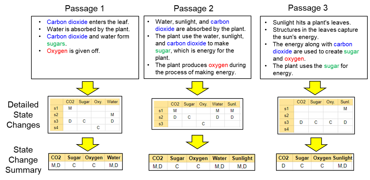
Figure 2: Three (simplified) passages from ProPara describing photosynthesis, the (gold) state changes each entity undergoes at each step $s_{1},s_{2},…,s_{T}$, and the summary of state changes that each entity undergoes (an aggregation of the step-by-step changes), where M = MOVED, D = DESTROYED, C = CREATED. Although the language and detailed changes for each passage differ considerably, the overall summaries are largely consistent (e.g., sugar is CREATED in all three). We exploit this consistency when training a model to make these predictions, by biasing the model to prefer predictions whose summary is consistent with the (predicted) summaries of other passages about the same topic. Note that in the summary, we do not care about the order in which state changes happen, so summary M, D for participant CO₂ in passage 1 denotes a set of state changes rather than a sequence of state changes.

Using multiple, distinct passages to understand a process or procedure is challenging. Although the texts describe the same process, they might express the underlying facts at different levels of granularity, using different wordings, and including or omitting different details. As a result, the details may differ between paragraphs, making them hard to align and to check for consistency. Nonetheless, even if the details differ, we conjecture that the top-level summaries of each paragraph, which describe the types of state change that each entity undergoes, will be mostly consistent. For example, although independent texts describing photosynthesis vary tremendously, we expect them to be consistent about what generally happens to sugar, e.g., that it is created (Figure 2).

In this paper, we introduce a new training framework, called LaCE (Label Consistency Explorer), that leverages label consistency among paragraph summaries. In particular, it encourages label consistency during end-to-end training of a neural model, allowing consistency bias to improve the model itself, rather than be enforced in a post-processing step, e.g., posterior regularization Ganchev et al. (2010). We evaluate on a standard benchmark for procedural text comprehension, called ProPara Dalvi et al. (2018). We show that this approach achieves a new state-of-the-art performance in the fully supervised setting (when all paragraphs are annotated), and also demonstrate that it improves performance in the semi-supervised setting (using additional, unlabeled paragraphs) with limited training data. In the latter case, summary predictions from labeled data act as noisy gold labels for the unlabeled data, allowing additional learning to occur. Our contributions are thus:

• A new learning framework, LaCE, applied to procedural text comprehension that improves the label consistency among different paragraphs on the same topic.

• Experimental results demonstrating that LaCE achieves state-of-the-art performance on a standard benchmark dataset, ProPara, for procedural text.

2 Related Work

Our work is related to several important branches of work in both NLP and ML, as we now summarize.

Leveraging Label Consistency Leveraging information about label consistency (i.e., similar instances should have consistent labels at a certain granularity) is an effective idea. It has been studied in computer vision Haeusser et al. (2017); Chen et al. (2018) and IR Clarke et al. (2001); Dumais et al. (2002). Learning by association Haeusser et al. (2017) establishes implicit cross-modal links between similar descriptions and leverage more unlabeled data during training. Schütze et al. (2018); Hangya et al. (2018) adapt the similar idea to exploit unlabeled data for the cross-lingual classification. We extend this line of research in two ways: by developing a framework allowing it to be applied to the task of structure prediction; and by incorporating label consistency into the model itself via end-to-end training, rather than enforcing consistency as a post-processing step.

Semi-supervised Learning Approaches Besides utilizing the label consistency knowledge, our learning framework is also able to use unlabeled paragraphs, which fits in the literature of semi-supervised learning approaches (for NLP). Zhou et al. (2003) propose an iterative label propagation algorithm similar to spectral clustering. Zhu et al. (2003) propose a semi-supervised learning framework via harmonic energy minimization for data graph. Talukdar et al. (2008) propose a graph-based semi-supervised label propagation algorithm for acquiring open-domain labeled classes and their instances from a combination of unstructured and structured text sources. Our framework extends these ideas by introducing the notion of groups (examples that are expected to be similar) and summaries (what similarities are expected), applied in an end-to-end-framework.

Procedural Text Understanding and Reading Comprehension There has been a growing interest in procedural text understanding/QA recently. The ProcessBank dataset Berant et al. (2014) asks questions about event ordering and event arguments for biology processes. bAbI Weston et al. (2015) includes questions about movement of entities, however it’s synthetically generated and with a small lexicon. Kiddon et al. (2015)’s RECIPES dataset introduces the task of predicting the locations of cooking ingredients, and Kiddon et al. (2016) for recipe generation. In this paper, we continue this line of exploration using ProPara, and illustrate how the previous two lines of work (label consistency and semi-supervised learning) can be integrated.

3 Problem Definition

3.1 Input and Output

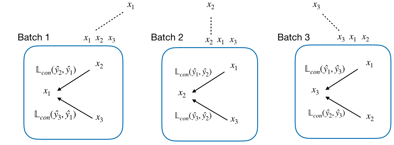
Figure 3: Example of batches constructed from a group (here, the group contains three labeled examples $x_{1},x_{2},x_{3}$). From three examples, three batches are constructed. Taking the predicted labels for the first element in the batch as reference we compute the consistency loss for the remaining elements.

A general condition for applying our method is having multiple examples where, for some properties, we expect to see similar values. For example, for procedural text, we expect paragraphs about the same process to be similar in terms of which entities move, are created, and destroyed; for different news stories about a political meeting, we expect top-level features (e.g., where the meeting took place, who attended) to be similar; for different recipes for the same item, we expect loosely similar ingredients and steps; and for different images of the same person, we expect some high-level characteristics (e.g., height, face shape) to be similar. Note that this condition does not apply to every learning situation; it only applies when training examples can be grouped, where all group members are expected to share some characteristics that we can identify (besides the label used to form the groups in the first place).

More formally, for training, the input is a set of labeled examples $(x_{gi},y_{gi})$ (where $y_{gi}$ are the labels for $x_{gi}$), partitioned into $G$ groups, where the $g$ subscript denotes which group each example belongs to. Groups are defined such that examples of the same group $g$ are expected to have similar labels for a subset of labels $y_{gi}$. We call this subset the summary labels. We assume that both the groupings and the identity of the summary labels are provided. The output of training is a model $M$ for labeling new examples. For testing, the input is the model $M$ and a set of unlabeled (and ungrouped) examples $x_{t}$, and the output are their predicted labels $\hat{y_{t}}$. Note that this formulation is agnostic to the learning algorithm used. Later, we will consider both the fully supervised setting (all training examples are labeled) and semi-supervised setting (only a subset are labeled).

3.2 Instantiation

We instantiate this framework for procedural text comprehension, using the ProPara task Dalvi et al. (2018). In this task, $x_{gi}$ are paragraphs of text describing a process (e.g., photosynthesis), the labels $y_{gi}$ describe the state changes that each entity in the paragraph undergoes at each step (sentence) (e.g., that oxygen is created in step 2), and the groups are paragraphs about the same topic (ProPara tags each paragraph with a topic, e.g., there are three paragraphs in ProPara describing photosynthesis). More precisely, each $x_{gi}$ consists of:

• the name (topic) of a process, e.g., photosynthesis

• a sequence (paragraph) of sentences $S=[s_{1},...,s_{T}]$ that describes that process

• the set of entities $E$ mentioned in that text, e.g., oxygen, sugar

and the targets (labels) to predict are:

• the state changes that each entity in $E$ undergoes at each step (sentence) of the process, where a state change is one of {Moved,Created,Destroyed,None}. These state changes can be conveniently expressed using a $|S|\times|E|$ matrix (Figure 2). State changes also include arguments, e.g., the source and destination of a move. We omit these in this paper to simplify the description.

Finally, we define the summary labels as the set of state changes that each entity undergoes at some point in the process, without concern for when. For example, in Passage 1 in Figure 2, CO₂ is Moved (M) and Destroyed (D), while sugar is Created (C). These summary labels can be computed from the state-change matrix by aggregating the state changes for each entity over all steps. Our assumption here is that these summaries will generally be the same (i.e., consistent) for different paragraphs about the same topic. LaCE then exploits this assumption by encouraging this inter-paragraph consistency during training, as we now describe.

4 Label Consistency Explorer: LaCE

4.1 The LaCE Learning Framework

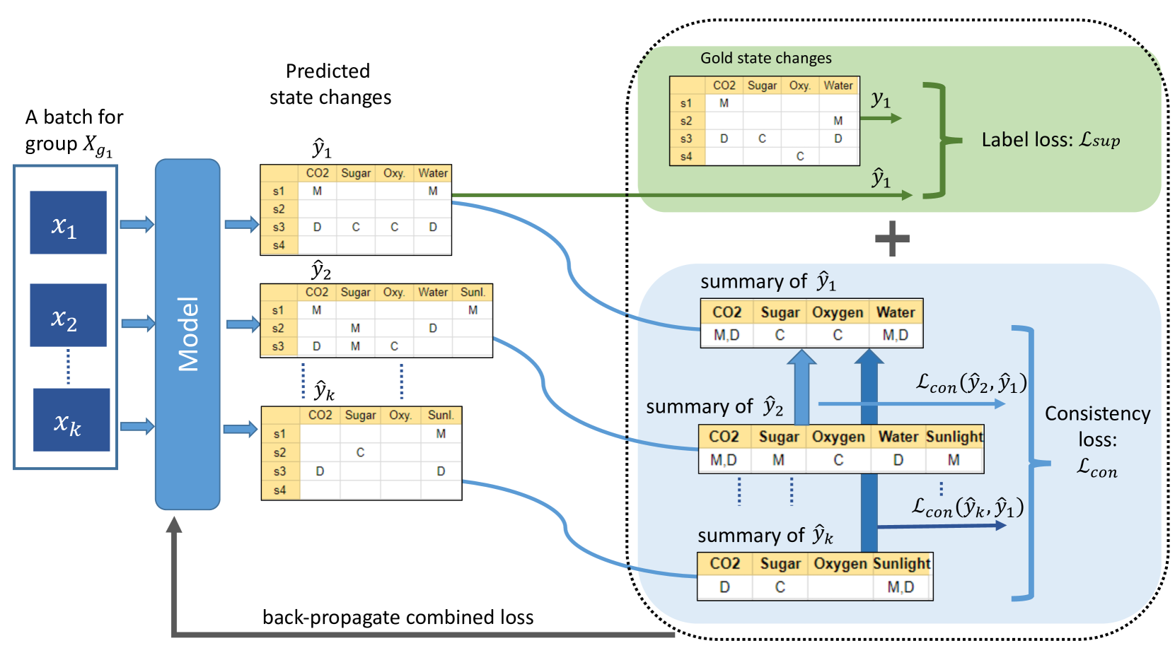
Figure 4: Overview of the LaCE training framework, illustrated for the procedural comprehension task ProPara. During training, LaCE processes batches of examples {$x_{1}$,…,$x_{k}$} for each group $X_{g}$, where predictions for one example (here $\hat{y_{1}}$) are compared against its gold (producing loss $\mathbb{L}_{sup}$), and its summary against summaries of all other examples to encourage consistency of predictions (producing $\mathbb{L}_{con}$), repeating for each example in the batch.

While a traditional supervised learning model operates on individual examples, LaCE operates on batches of grouped examples $X_{g}$. Given a group $g$ containing $N$ labeled examples $\{x_{1},...,x_{N}\}$ (we drop the $g$ subscript for clarity), LaCE creates $N$ batches, each containing all the examples but with a different $x_{i}$ labeled as “primary”, along with the gold labels $y_{i}$ for (only) the primary example. (We informally refer to the primary example as the “first example” in each batch). Then for each batch, LaCE jointly optimizes the usual supervised loss $\mathbb{L}_{sup}(\hat{y_{i}},y_{i})$ for the primary example, along with a consistency loss between (summary) predictions for all other members of the group and the primary example, $\mathbb{L}_{con}(\hat{y_{j}},\hat{y_{i}})$ for all $j\neq i$. This is illustrated in Figures 4 and 3. This is repeated for all batches.

For example, for the three paragraphs about photosynthesis (Figure 2), batch 1 compares the first paragraph’s predictions with its gold labels, and also compares the summary predictions of paragraphs 2 and 3 with those of the first paragraph (Figure 3). This is then repeated using paragraph 2, then paragraph 3 as primary.

The result is that LaCE jointly optimizes the supervised loss $\mathbb{L}_{sup}$ and consistency loss $\mathbb{L}_{con}$ to train a model that is both accurate for the given task as well as consistent in its predictions across examples that belong to the same group.

This process is approximately equivalent to jointly optimizing the usual supervised loss $\mathbb{L}_{sup}(\hat{y_{i}},y_{i})$ for all examples in the group, and the pairwise consistency loss $\mathbb{L}_{con}(\hat{y_{j}},\hat{y_{i}})$ for all pairs $(x_{j},x_{i}),{\color[rgb]{0,0,0}j\neq i}$ in the group. However, there is an important difference, namely the relative contributions of $\mathbb{L}_{sup}$ and $\mathbb{L}_{con}$ is varied among batches, depending on how accurate the predictions for the primary example are (i.e., how small $\mathbb{L}_{sup}$ is), as we describe later in Section 4.3. This has the effect of paying more attention to consistency loss when predictions on the primary are more accurate.

We also extend LaCE to the semi-supervised setting as follows. For the semi-supervised setting, where only $m$ of $n$ $(m<n)$ examples are labeled, we only form $m$ batches, where each batch has a different labeled example as primary. We later report experiments results for both the fully and semi-supervised settings.

4.2 Base Model for Procedural Text

We now describe how LaCE is applied to our goal of comprehending procedural text. Note that LaCE is agnostic to the learner used within the framework. For this application, we use a simplified version of ProStruct Tandon et al. (2018), a publicly available system designed for the ProPara task. Our implementation simplifies ProStruct by reusing its encoder, but then predicting (a distribution over) each state change label independently during decoding for every cell in the $|S|\times|E|$ grid (Figure 2). We briefly summarize this here.

4.2.1 Encoder

ProStruct uses an encoder-decoder architecture that takes procedural text as input and predicts the state changes of entities $E$ in the text as output. During encoding, each step $s_{t}$ is encoded using $|E|$ embeddings, one for each entity $e_{j}\in E$. Each embedding represents the action that $s_{t}$ describes, applied to $e_{k}$. The model thus allows the same action to have different effects on different entities (e.g., a transformation destroys one entity, and creates another).

For each $(s_{t},e_{j})\in S\times E$ pair, the step is fed into a BiLSTM Hochreiter and Schmidhuber (1997), using pretrained GloVe Pennington et al. (2014) vectors $v_{w}$ for each word $w_{i}$ concatenated with two indicator variables, one indicating whether $w_{i}$ is a word referring to $e_{j}$, and one indicating whether $w_{i}$ is a verb. A bilinear attention layer then computes attention over the contextualized vectors $h_{i}$ output by the BiLSTM: $a_{i}=h_{i}*B*h_{ev}+b$ , where $B$ and $b$ are learned parameters, and $h_{ev}$ is the concatenation of $h_{e}$ (the averaged contextualized embedding for the entity words $w_{e}$) and $h_{v}$ (the averaged contextualized embedding for the verb words $w_{v}$).

Finally, the output vector $c_{tj}$ is the attention-weighted sum of the $h_{i}$: $c_{tj}=\sum_{i=1}^{I}a_{i}*h_{i}$ . Here, $c_{tj}$ can be thought of as representing the action $s_{t}$ applied to entity $e_{j}$. This is repeated for all steps and entities.

4.2.2 Decoder

To decode the action vectors $c_{tj}$ into their resulting state changes they imply, each is passed through a feedforward layer to generate $logit(\pi_{tj})$, a set of logistic activations over the $K$ possible state changes $\pi_{tj}$ for entity $e_{j}$ in step $s_{t}$. For ProPara, there are $K=4$ possible state changes: Move, Create, Destroy, and None. These logits form a distribution over possible state changes to predict, for each entity and step in the text. We then compute loss, described next, using these distributions directly rather than discretizing them into exact predictions at this stage, so as not to lose information.

4.3 Applying LaCE

4.3.1 Batching

We start by creating training batches for each $X_{g_{i}}\in X_{g}$. From a group $X_{g_{i}}$ comprising of $n$ examples, we create $n$ training batches. A batch consists of all $n$ examples $(x_{1},x_{2},...,x_{n})$, but the loss computation is different in each batch. Figure 3 illustrates this.

4.3.2 Loss Computation

The loss computation in a batch is based on the usual supervised loss and additionally the consistency loss, as follows:

$$\mathbb{L}_{batch} =\lambda\underbrace{\mathbb{L}_{sup}(\hat{y_{1}},y_{1})}_{supervised~{}loss}~{}+(1-\lambda)\underbrace{\sum_{i=2}^{n}\mathbb{L}_{con}(\hat{y_{i}},\hat{y_{1}})}_{consistency~{}loss}$$ (1)

Here, $\mathbb{L}_{sup}(\hat{y_{1}},y_{1})$ is the negative log likelihood loss against the gold labels $y_{1}$, and $\lambda$ is a hyperparameter tuned on the dev set.

To compute the consistency loss $\mathbb{L}_{con}(\hat{y_{i}},\hat{y_{1}})$, we compare the summaries computed from $\hat{y_{i}}$ and $\hat{y_{1}}$. In our particular application, a summary lists all the state changes each entity undergoes, formed by aggregating its step-by-step state changes. For example, for paragraph $x_{1}$ in Figure 4, as CO₂ first moves (M), then later is destroyed (D), we summarize its state changes as $s(\texttt{CO}_{2},\hat{y}_{1})$ = {M,D}. In practice, as our decoder outputs distributions over the four possible values {M,C,D,N} rather than a single value, we summarize by adding and normalizing these distributions, producing a summary distribution $s(e,\hat{y}_{j})$ over the four values rather than a discrete set of values.

To compute the consistency loss $\mathbb{L}_{con}(\hat{y_{i}},\hat{y_{1}})$ itself, we compare summaries for each entity $e$ that occurs in both paragraph ${x_{1}}$ and paragraph $x_{i}$ (referred to as Ent($x_{1}$) and Ent($x_{i}$) respectively), and compute the average mean squared error (MSE) between their summary distributions. We also tried other alternatives (e.g., Kullback-Leibler divergence) for calculating the distance between summary distributions, but mean squared error performs best. Equation 2 shows the details for computing the consistency loss.

$$\mathbb{L}_{con}(\hat{y_{i}},\hat{y_{1}}) =\frac{\sum_{e\in Ent(x_{i})\cap Ent(x_{1})}\textrm{MSE}(s(e,\hat{y}_{i}),s(e,\hat{y}_{1}))}{|Ent(x_{i})\cap Ent(x_{1})|}$$ (2)

Note that each paragraph contains varying number of entities and sentences. It is possible that some paragraphs do not mention exactly the same entities as the labeled paragraph (first element in the batch). In such cases, we penalize the model only for predictions for co-occurring entities. Unmatched entities are not penalized.

4.3.3 Adaptive Loss

The supervised loss $\mathbb{L}_{sup}(\hat{y_{1}},y_{1})$ is large in the early epochs when the model is not sufficiently trained. At this point, it is beneficial for the model to pay no attention to the consistency loss $\mathbb{L}_{con}(\hat{y_{j}},\hat{y_{1}})$ as the predicted action distributions are inaccurate. To implement this, if $\mathbb{L}_{sup}$ is above a defined threshold then the consistency loss term in Equation 1 is ignored (i.e. $\lambda=1$). Otherwise, Equation 1 is used as is. This can loosely be seen as a form of simulated annealing Kirkpatrick et al. (1988), using just two temperatures. Note that the time (epoch number) when the temperature (lambda) changes will vary across batches depending on the supervised loss within that batch of data, hence we call it an “adaptive” loss.

5 Experimental Results

We now present results on ProPara, the procedural text comprehension dataset introduced in Dalvi et al. (2018). There are 187 topics in this dataset and a total of 488 labeled paragraphs (around 3 labeled paragraphs per topic). The task is to track how entities change state through the paragraph (as described in Section 3.2) and answer 4 classes of questions about those changes (7043/913/1095 questions in each of the train/dev/test partitions respectively). We compare LaCE with the baselines and prior state-of-the-art model ProStruct Tandon et al. (2018) in two settings: (1) Fully supervised learning (using all the training data). (2) Semi-supervised learning (using some or all of the training data, plus additional unlabeled data).

5.1 Fully Supervised Learning

Models	P	R	F1
EntNet Henaff et al. (2017)	54.7	30.7	39.4
QRN Seo et al. (2017)	60.9	31.1	41.1
ProLocal Dalvi et al. (2018)	81.7	36.8	50.7
ProGlobal Dalvi et al. (2018)	61.7	44.8	51.9
ProStruct Tandon et al. (2018)	74.3	43.0	54.5
LaCE (our model)	75.3	45.4	56.6

Table 1: Comparing the performance of LaCE with prior methods on the test partition of ProPara.

We evaluated LaCE by comparing its performance against published, state-of-the-art results on ProPara, using the full training set to train LaCE. The results are shown in Table 1. In Table 1, all the baseline numbers are the results reported in Tandon et al. (2018). Note that all these baselines are trying to reduce the gap between predicted labels and gold labels on the training dataset. LaCE, however, also optimizes for consistency across labels for groups of paragraphs belonging to the same topic. As LaCE uses parts of ProStruct as its learning algorithm, the gains over ProStruct appear to be coming directly from its novel learning framework described in Section 4.1. To confirm this, we also performed an ablation study, removing the consistency loss term and just using the base model in LaCE. The results are shown in Table 2, and show that the F1 score drops from 56.6 to 53.2, illustrating that the consistency loss is responsible for the improvement. In addition, Table 2 indicates that consistency loss helps improve both precision and recall.

Also note that LaCE simplifies parts of ProStruct. For example, unlike ProStruct, LaCE does not use a pre-computed knowledge base during decoding. Thus LaCE is more efficient to train than ProStruct (>15x faster at training time).

Finally, LaCE builds upon ProStruct (state-of-the-art when we started working on our model). Since LaCE was developed, two higher results of 57.6 and 62.5 on the ProPara task have appeared Das et al. (2019); Gupta and Durrett (2019). Both systems are fully supervised and developed contemporaneously with LaCE. In principle LaCE’s approach of leveraging consistency across paragraphs to train a more robust model can be applied to other systems. Our main contribution is to show that maximizing consistency across datapoints (in addition to minimizing supervised loss) enables a model to leverage unlabeled data and leads to more robust results.

Models	P	R	F1
LaCE	75.3	45.4	56.6
- consistency loss $\mathbb{L}_{con}$	69.6	43.1	53.2

Table 2: LaCE ablation results

Models	Proportion of labeled paragraphs
	used per training topic
	33%	66%	100%
ProStruct	45.4	50.6	54.5
LaCE	47.3	51.2	56.6
LaCE + unlabeled data	49.9	52.9	56.7

Table 3: Comparing LaCE vs. ProStruct with varying amount of labeled paragraphs available per training topic. We compare their performance in terms of F1 on ProPara test partition.

5.2 Semi-Supervised Learning

Unlike the other systems in Table 1, LaCE is able to use unlabeled data during training. As described in Section 4.1, given a group containing both labeled and unlabeled paragraphs, we create as many batches as the number of labeled paragraphs in the group. Hence, paragraphs $x_{i}$ with gold labels $y_{i}$ can contribute to both supervised loss $\mathbb{L}_{sup}$ and consistency loss $\mathbb{L}_{con}$. Additionally, we can use unlabeled paragraphs $x_{j}$ (i.e., without gold labels $y_{j}$), while computing consistency loss $\mathbb{L}_{con}$. This way LaCE can make use of unlabeled data during training.

To evaluate this, we collected 877 additional unlabeled paragraphs for ProPara topics. As the original ProPara dataset makes some simplifying assumptions, in particular that events are mentioned in chronological order, we used Mechanical Turk to collect additional paragraphs that conformed to those assumptions (rather than collecting paragraphs from Wikipedia, say). Approximately 3 extra paragraphs were collected for each topic in ProPara. Note that collecting unlabeled paragraphs is substantially less expensive than labeling paragraphs.

	Train	Dev	Test	Unlabeled
# paragraphs	391	54	43	877

Table 4: ProPara Paragraphs Statistics

We then trained the ProStruct and LaCE models varying two different parameters: (1) the percentage of the labeled (ProPara) training data used to train the system (2) for LaCE only, whether the additional unlabeled data was also used. This allows us to see performance under different conditions of sparsity of labeled data, and (for LaCE) also assess how much unlabeled data can help under those conditions. During training, the unused labeled data was ignored (not used as unlabeled data). We keep the dev and test partitions the same as original dataset, picking a model based on dev performance and report results on test partition. The results are shown in Table 3. In the first two rows, ProStruct and LaCE are both trained with x% of labeled data, while the last row reports performance of LaCE when it also has access to new unlabeled paragraphs.

Table 3 demonstrates that LaCE results in even larger improvements over ProStruct when the amount of labeled data is limited. In addition, unlabeled data adds an additional boost to this performance, in particular when labeled data is sparse. Further examination suggests that the gains in F1 are resulting mainly from improved recall, as shown in Figure 5. We believe that having access to unlabeled paragraphs and optimizing consistency across paragraphs for training topics, helps LaCE generalize better to unseen topics.

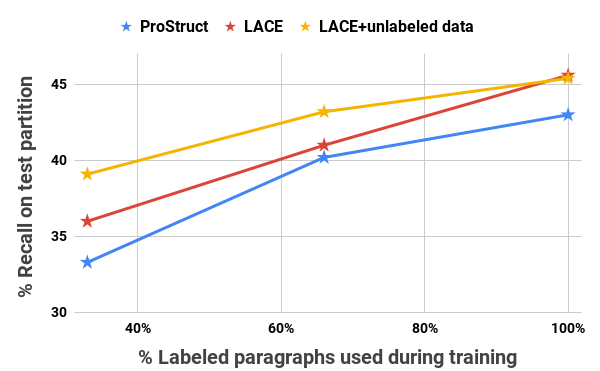
Figure 5: Comparing LaCE vs. ProStruct based on Recall on the test partition, by varying amount of labeled paragraphs available per training topic

5.3 Implementation Details for LaCE

We implement our proposed model LaCE in PyTorch Paszke et al. (2017) using the AllenNLP Gardner et al. (2018) toolkit. We added a new data iterator that creates multiple batches per topic (Figure 3) which enables easy computation of consistency loss. We use 100D Glove embeddings Pennington et al. (2014), trained on Wikipedia 2014 and Gigaword 5 corpora (6B tokens, 400K vocab, uncased). Starting from glove embeddings appended by entity and verb indicators, we use bidirectional LSTM layer to create contextual representation for every word in a sentence. We use 100D hidden representations for the bidirectional LSTM Hochreiter and Schmidhuber (1997) shared between all inputs (each direction uses 50D hidden vectors). We use attention layer on top of BiLSTM, using a bilinear similarity function similar to Chen et al. (2016) to compute attention weights over the contextual embedding for each word in the sentence.

To compute the likelihood of all state changes individually, we use a single layer feedforward network with input dimension of 100 and output 4. In these experiments, we check if the supervised loss $\mathbb{L}_{sup}$ is less than a threshold (0.2 in our case) then we use equation 1 and $lambda=0.05$. All hyper-parameters are tuned on the dev data.

During training we use multiple paragraphs for a topic to optimize for both supervised and consistency loss. At test time, LaCE’s predictions are based on only one given paragraph. All the performance gains are due to the base model being more robust due to proposed training procedure. The code for LaCE model is published at https://github.com/allenai/propara.

5.4 Analysis and Discussion

We first discuss the predicted label consistency across paragraphs for LaCE vs. ProStruct. We then identify some of the limitations of LaCE.

Label Consistency

	Consistency Score (%)
	Train	Test
ProStruct	46.70	37.21
LaCE	54.39	38.36

Table 5: Consistency score comparison

LaCE attempts to encourage consistency between paragraphs about the same topic during training, and yield similar benefit at test time. To examine whether this happens in practice, we compute and report the consistency score between paragraphs about the same topic (Table 5). Specifically, for an entity that appears in two paragraphs about the same topic, we compare whether the summaries of state change predictions for each match. The results are shown in Table 5.

The table shows that LaCE achieves greater prediction consistency during training, and that this benefit plays out to some extent at test time even though label consistency is not enforced at test time (we do not assume that examples are grouped at test time, hence consistency between groups cannot be enforced as the grouping is unknown). As an illustration, for the topic describe the life cycle of a tree which is unseen at training time, for the three paragraphs on the topic, ProStruct predicts that tree is created; not-changed; and created respectively, while LaCE correctly predicts that tree is created; created; and created respectively. This illustrates a case where LaCE has learned to make predictions that are more consistent and correct.

Error Analysis for LaCE

To understand LaCE’s behavior further, we examined cases where LaCE’s and ProStruct’s predictions differ, and examined their agreement with gold labels. In this analysis we found three major sources of errors for LaCE:

• The label consistency assumption does not always hold: In Section 3.1, we explain that LaCE relies on summary labels being consistent across examples in the same group. We found that for some of the topics in our training dataset this assumption is sometimes violated. E.g., for the topic How does the body control its blood sugar level?, there are two different paragraphs; one of them describes the entity sugar as being Created and then Destroyed to create bloodsugar, while the other paragraph describes the same event in a different way by saying that the entity sugar is Created and then Moved to the blood. LaCE can thus goes wrong when trying to enforce consistency in such cases.

• Lexical variance between entities across paragraphs: Different paragraphs about the same topic may describe the procedure using different wordings, resulting in errors. For example, in paragraphs about the topic what happens during photosynthesis?, the same entity (carbon dioxide) is referred to by two different strings, CO₂ in one paragraph and carbon dioxide in another. Currently, LaCE does not take into account entity synonyms, so it is unable to encourage consistency here. An interesting line of future work would be to use the embedding space similarity between entity names, to help address this problem.

• LaCE can make incorrect predictions to improve consistency: For the topic Describe how to make a cake at training time, when presented with two paragraphs, LaCE tries to be consistent and incorrectly predicts that cake is Destroyed in both paragraphs. ProStruct does not attempt to improve prediction consistency, here resulting in less consistent but in this case more accurate predictions for this topic.

5.5 Directions For Enhancing LaCE

• Improve LaCE for ProPara: LaCE’s performance on ProPara can be improved further by a) soft matching of entities across paragraphs instead of current exact string match b) exploring more systematic ways (e.g., simulated annealing) to define adaptive loss c) using additional sources of unlabeled data (e.g., web, textbooks) weighed by their reliability.

• Apply LaCE on other tasks: Architecturally, LaCE is a way to train any existing structured prediction model for a given task to produce consistent labels across similar datapoints. Hence it can be easily applied to other tasks where parallel data is available (grouping function) and there is a way to efficiently compare predictions (summary labels) across parallel datapoints, e.g. event extraction from parallel news articles Chinchor (2002).

  Further, summary labels need not be action categories (e.g., Created, Destroyed). Consistency can also be computed for QA task where multiple parallel text is available for reading comprehension. We plan to explore this direction in the future.

6 Conclusion

Our goal is procedural text comprehension, a task that current systems still struggle with. Our approach has been to exploit the fact that, for many procedures, multiple independent descriptions exist, and that we expect some consistency between those descriptions. To do this, we have presented a task- and model-general learning framework, LaCE, that can leverage this expectation, allowing consistency bias to be built into the learned model. Applying this framework to procedural text, the resulting system obtains new state-of-the-art results on the ProPara dataset, an existing benchmark for procedural text comprehension. It also demonstrates the ability to benefit from unlabeled paragraphs (semi-supervised learning), something that prior systems for this task were unable to do. We have also identified several avenues for further improvement (Section 5.4), and are optimistic that further gains can be achieved.

Acknowledgements

Computations on beaker.org were supported in part by credits from Google Cloud.

References

- Berant et al. (2014) Jonathan Berant, Vivek Srikumar, Pei-Chun Chen, Abby Vander Linden, Brittany Harding, Brad Huang, Peter Clark, and Christopher D Manning. 2014. Modeling biological processes for reading comprehension. In Proc. EMNLP’14.
- Bosselut et al. (2018) Antoine Bosselut, Omer Levy, Ari Holtzman, Corin Ennis, Dieter Fox, and Yejin Choi. 2018. Simulating action dynamics with neural process networks. 6th International Conference on Learning Representations (ICLR).
- Chen et al. (2016) Danqi Chen, Jason Bolton, and Christopher D. Manning. 2016. A thorough examination of the cnn/daily mail reading comprehension task. CoRR, abs/1606.02858.
- Chen et al. (2018) Kevin Chen, Christopher B. Choy, Manolis Savva, Angel X. Chang, Thomas A. Funkhouser, and Silvio Savarese. 2018. Text2shape: Generating shapes from natural language by learning joint embeddings. CoRR, abs/1803.08495.
- Chinchor (2002) Nancy A. Chinchor. 2002. Message understanding conference ( muc ) tests of discourse processing.
- Clarke et al. (2001) Charles LA Clarke, Gordon V Cormack, and Thomas R Lynam. 2001. Exploiting redundancy in question answering. In Proceedings of the 24th annual international ACM SIGIR conference on Research and development in information retrieval. ACM.
- Dalvi et al. (2018) Bhavana Dalvi, Lifu Huang, Niket Tandon, Wen-tau Yih, and Peter Clark. 2018. Tracking state changes in procedural text: A challenge dataset and models for process paragraph comprehension. NAACL-HLT’18, arXiv preprint arXiv:1805.06975.
- Das et al. (2019) Rajarshi Das, Tsendsuren Munkhdalai, Xingdi Yuan, Adam Trischler, and Andrew McCallum. 2019. Building dynamic knowledge graphs from text using machine reading comprehension. ICLR. ArXiv:1810.05682.
- Dumais et al. (2002) Susan T. Dumais, Michele Banko, Eric Brill, Jimmy J. Lin, and Andrew Y. Ng. 2002. Web question answering: is more always better? In SIGIR.
- Ganchev et al. (2010) Kuzman Ganchev, João Graça, Jennifer Gillenwater, and Ben Taskar. 2010. Posterior regularization for structured latent variable models. Journal of Machine Learning Research, 11:2001–2049.
- Gardner et al. (2018) Matt Gardner, Joel Grus, Mark Neumann, Oyvind Tafjord, Pradeep Dasigi, Nelson Liu, Matthew Peters, Michael Schmitz, and Luke Zettlemoyer. 2018. Allennlp: A deep semantic natural language processing platform. arXiv preprint arXiv:1803.07640.
- Gupta and Durrett (2019) Aditya Gupta and Greg Durrett. 2019. Tracking discrete and continuous entity state for process understanding. arXiv preprint arXiv:1904.03518. (To appear in NAACL’19 workshop on Structured Prediction for NLP).
- Haeusser et al. (2017) Philip Haeusser, Alexander Mordvintsev, and Daniel Cremers. 2017. Learning by association-a versatile semi-supervised training method for neural networks. In IEEE Conference on Computer Vision and Pattern Recognition (CVPR), volume 3, page 6.
- Hangya et al. (2018) Viktor Hangya, Fabienne Braune, Alexander Fraser, and Hinrich Schütze. 2018. Two methods for domain adaptation of bilingual tasks: Delightfully simple and broadly applicable. In Proceedings of the 56th Annual Meeting of the Association for Computational Linguistics (Volume 1: Long Papers).
- Henaff et al. (2017) Mikael Henaff, Jason Weston, Arthur Szlam, Antoine Bordes, and Yann LeCun. 2017. Tracking the world state with recurrent entity networks. In ICLR.
- Hochreiter and Schmidhuber (1997) Sepp Hochreiter and Jürgen Schmidhuber. 1997. Long short-term memory. Neural computation, 9(8):1735–1780.
- Kiddon et al. (2015) Chloé Kiddon, Ganesa Thandavam Ponnuraj, Luke Zettlemoyer, and Yejin Choi. 2015. Mise en place: Unsupervised interpretation of instructional recipes. In Proc. EMNLP’15.
- Kiddon et al. (2016) Chloé Kiddon, Luke Zettlemoyer, and Yejin Choi. 2016. Globally coherent text generation with neural checklist models. In Proc. EMNLP’16.
- Kirkpatrick et al. (1988) Scott Kirkpatrick, C. D. Gelatt, and Mario P. Vecchi. 1988. Optimization by simulated annealing.
- Paszke et al. (2017) Adam Paszke, Sam Gross, Soumith Chintala, Gregory Chanan, Edward Yang, Zachary DeVito, Zeming Lin, Alban Desmaison, Luca Antiga, and Adam Lerer. 2017. Automatic differentiation in pytorch.
- Pennington et al. (2014) Jeffrey Pennington, Richard Socher, and Christopher Manning. 2014. Glove: Global vectors for word representation. In Proceedings of the 2014 conference on empirical methods in natural language processing (EMNLP), pages 1532–1543.
- Schütze et al. (2018) Hinrich Schütze, Fabienne Braune, Alexander M. Fraser, and Viktor Hangya. 2018. Two methods for domain adaptation of bilingual tasks: Delightfully simple and broadly applicable. In ACL.
- Seo et al. (2017) Minjoon Seo, Sewon Min, Ali Farhadi, and Hannaneh Hajishirzi. 2017. Query-reduction networks for question answering. In ICLR.
- Talukdar et al. (2008) Partha Pratim Talukdar, Joseph Reisinger, Marius Pasca, Deepak Ravichandran, Rahul Bhagat, and Fernando Pereira. 2008. Weakly-supervised acquisition of labeled class instances using graph random walks. In EMNLP.
- Tandon et al. (2018) Niket Tandon, Bhavana Dalvi Mishra, Joel Grus, Wen-tau Yih, Antoine Bosselut, and Peter Clark. 2018. Reasoning about actions and state changes by injecting commonsense knowledge. EMNLP’18, arXiv preprint arXiv:1808.10012.
- Weston et al. (2015) Jason Weston, Antoine Bordes, Sumit Chopra, Alexander M Rush, Bart van Merriënboer, Armand Joulin, and Tomas Mikolov. 2015. Towards AI-complete question answering: A set of prerequisite toy tasks. arXiv preprint arXiv:1502.05698.
- Zhou et al. (2003) Dengyong Zhou, Olivier Bousquet, Thomas Navin Lal, Jason Weston, and Bernhard Schölkopf. 2003. Learning with local and global consistency. In NIPS.
- Zhu et al. (2003) Xiaojin Zhu, Zoubin Ghahramani, and John D Lafferty. 2003. Semi-supervised learning using gaussian fields and harmonic functions. In Proceedings of the 20th International conference on Machine learning (ICML), pages 912–919.