Quasiexact Kondo Dynamics of Fermionic Alkaline-Earth-Like Atoms at Finite Temperatures

Abstract

A recent experiment has observed the antiferromagnetic interaction between the ground state ${}^{1}S_{0}$ and the metastable state ${}^{3}P_{0}$ of ¹⁷¹Yb atoms, which are fermionic. This observation combined with the use of state-dependent optical lattices allows for quantum simulation of the Kondo model. We propose that in this Kondo simulator the anomalous temperature dependence of transport, namely the Kondo effect, can be detected through quench dynamics triggered by the shift of a trap potential. For this purpose, we improve the numerical efficiency of the minimally entangled typical thermal states (METTS) algorithm by applying additional Trotter gates. Using the improved METTS algorithm, we compute the quench dynamics of the one-dimensional Kondo model at finite temperatures quasi-exactly. We find that the center-of-mass motion exhibits a logarithmic suppression with decreasing the temperature, which is a characteristic feature of the Kondo effect.

Orbital degrees of freedom are a fundamental element for understanding physics of various condensed matter systems, including heavy-fermion materials Steglich et al. (1979); Stewart (1984), transition metal oxides Falicov and Kimball (1969); Kugel and Khomskii (1980); Tokura and Nagaosa (2000), iron pnictides Kamihara et al. (2008); Kuroki et al. (2008); Si et al. (2016), and compound semiconductors Byrnes et al. (2014); Kuneš (2015). In these systems, the multiorbital character, together with the spin degrees of freedom and strong interparticle interactions, leads to the emergence of magnetism, superconductivity, excitonic condensation, and the Kondo effect. It is widely believed that the essence of some of these properties can be extracted by analyzing the two-orbital Anderson- and Kondo-type models, in which delocalized fermions in one orbital exchanges their spins with localized fermions in the other orbital. However, accurate simulation of these models with classical resources is in general intractable because of the exponential growth of the Hilbert space and the minus sign problem in quantum Monte Carlo simulations.

An alternative approach for analyzing the prototypical two-orbital models is analog quantum simulation Feynman (1982) using optical lattices loaded with ultracold gases Bloch et al. (2012); Gross and Bloch (2017); Hofstetter and Qin (2018). It has been proposed that optical-lattice quantum simulators (OLQSs) of the two-orbital models can be realized with use of fermionic alkaline-earth-like atoms (AEAs) Gorshkov et al. (2010); Foss-Feig et al. (2010); Nakagawa and Kawakami (2015); Zhang et al. (2016); Cheng et al. (2017), such as strontium DeSalvo et al. (2010) and ytterbium Fukuhara et al. (2007); Taie et al. (2010). A remarkable advantage of AEAs over alkali atoms is the existence of the electronically excited state ${}^{3}P_{0}$ or ${}^{3}P_{2}$ with long lifetime, which can be coupled to the ground state ${}^{1}S_{0}$ via an ultranarrow clock transition. Riegger et al. indeed have used a state-dependent optical lattice to create a two-orbital fermionic quantum gas of ¹⁷³Yb Riegger et al. (2018), in which atoms in ${}^{1}S_{0}$ (${}^{3}P_{0}$) state play a role of delocalized (localized) fermions. Moreover, Ono et al. have reported the observation of antiferromagnetic spin-exchange interaction between the ${}^{1}S_{0}$ and ${}^{3}P_{0}$ states of ¹⁷¹Yb Ono et al. (2019). Since ¹⁷¹Yb atoms in the ${}^{1}S_{0}$ state hardly interact with each other Kitagawa et al. (2008), their two-orbital system in a state-dependent optical lattice naturally simulates the Kondo model.

One of the most important targets of the OLQS of the Kondo model is the Kondo effect Kondo (1964); Abrikosov (1965); Yosida (1966); Anderson (1970); Wilson (1975); Andrei et al. (1983), in which a localized fermion forms a many-body spin-singlet state with delocalized fermions when the temperature is lowered. The formation of such Kondo singlets causes the anomalous increase of the resistance with decreasing the temperature. The Kondo effect is thought to be a key concept for understanding rich quantum phases and phase transitions of the Kondo lattice model represented by a Doniach phase diagram Doniach (1977). Since transport properties of trapped quantum gases have been often investigated by measuring their center-of-mass (COM) motion induced in response to a sudden displacement of the trapping potential Burger et al. (2001); Fertig et al. (2005); Strohmaier et al. (2007); McKay et al. (2008); Haller et al. (2010); Tanzi et al. (2016); Boéris et al. (2016), it is likely that the Kondo effect in the OLQS of the Kondo model will be detected via such simple transport measurements. However, accurate theoretical predictions on the COM dynamics have never been made because of the difficulties in calculating real-time evolution of the quantum many-body system with two orbitals at finite temperatures.

In this letter, we develop a numerical method that overcomes such difficulties in order to show that the Kondo effect of the Kondo OLQS can be indeed detected by measuring the COM motion of the delocalized fermions after the trap displacement. Specifically, we restrict ourselves to one-dimensional (1D) systems, in which matrix product states (MPS) serve as an efficient description of states with relatively low energy White (1992, 1993); Schollwöck (2011), and modify the finite-temperature algorithm using the minimally entangled typical thermal states (METTS) White (2009); Stoudenmire and White (2010). Our modified METTS algorithm includes additional Trotter gates and allows for efficient simulations of systems with an Abelian symmetry, such as the Hubbard and Kondo models. Using the modified METTS, we compute the finite temperature dynamics of the Kondo model with the antiferromagnetic interaction and find that when the temperature decreases, the maximum COM speed during the dynamics logarithmically decreases, i.e., the transport exhibits a logarithmic suppression, which is a characteristic feature of the Kondo effect. We also analyze the fully spin-polarized system and the ferromagnetic Kondo model, in which the Kondo effect does not occur Furusaki (2005), as references to be compared with the antiferromagnetic case. The logarithmic suppression of the transport is found to be absent in these two cases.

Model and method.— We consider an ultracold mixture of ¹⁷¹Yb atoms, which are fermionic, in the ${}^{1}S_{0}$ and ${}^{3}P_{0}$ states confined in a combined potential of optical lattices and a parabolic trap. We assume that the transverse optical lattice is sufficiently deep such that the system can be regarded to be spatially 1D. The longitudinal optical lattice is state dependent in a way that an atom in the ${}^{3}P_{0}$ state is localized at $j=0$ while the lattice for ${}^{1}S_{0}$ atoms is modestly deep for the tight-binding approximation to be valid but is shallow enough to make ${}^{1}S_{0}$ atoms delocalized. This system is well described by the 1D Kondo model Kasuya (1956); Kondo (1964) with a parabolic trap term,

$$\hat{H}= -J\sum^{L-1}_{i=-L}\sum_{\sigma}\left(\hat{c}^{\dagger}_{i\sigma}\hat{c}_{i+1\sigma}+\mathrm{H.c.}\right)+V\hat{\bm{s}}_{i=0}\cdot\hat{\bm{S}}_{\mathrm{imp}}$$ (1)

$$+w\sum^{L}_{i=-L}\sum_{\sigma}{(i-x_{\mathrm{c}}/a)}^{2}\hat{n}_{i\sigma},$$

and can be regarded as an OLQS of the model. The total number of sites is $2L+1$. Here, $\hat{c}^{\dagger}_{i\sigma}$ ($\hat{c}_{i\sigma}$) creates (annihilates) a ${}^{1}S_{0}$ fermion with spin $\sigma$ at site $i$, and $\hat{n}_{i\sigma}=\hat{c}^{\dagger}_{i\sigma}\hat{c}_{i\sigma}$. $\hat{\bm{s}}_{i}=(\hat{s}^{x}_{i},\hat{s}^{y}_{i},\hat{s}^{z}_{i})$ are spin operators of a ${}^{1}S_{0}$ fermion at site $i$ and each component is defined as $\hat{s}^{\gamma}=(1/2)\sum_{\alpha\beta}\hat{c}^{\dagger}_{i\alpha}\sigma^{\gamma}_{\alpha\beta}\hat{c}_{i\beta}$ with the Pauli matrices $\bm{\sigma}^{\gamma}$. $\hat{\bm{S}}_{\mathrm{imp}}=(\hat{S}^{x}_{\mathrm{imp}},\hat{S}^{y}_{\mathrm{imp}},\hat{S}^{z}_{\mathrm{imp}})$ are spin operators of the impurity fermion at site $0$. $J$ denotes the hopping amplitude of ${}^{1}S_{0}$ fermions, $V$ the spin-exchange interaction between ${}^{1}S_{0}$ and ${}^{3}P_{0}$ fermions, $w$ the amplitude of the trap, $x_{\mathrm{c}}$ the position of the trap center, and $a$ the lattice constant.

The interaction between ¹⁷¹Yb atoms in the ${}^{1}S_{0}$ state can be safely ignored because it is very small (the $s$-wave scattering length is $a_{s}=-0.15\,{\rm nm}$ Kitagawa et al. (2008)). It is worth noting that there exists direct interaction between ${}^{1}S_{0}$ and ${}^{3}P_{0}$ fermions, which is given by $V_{\mathrm{d}}(\sum_{\sigma}\hat{n}_{i=0\sigma})\hat{n}_{\mathrm{imp}}$ Ono et al. (2019). Since the number of a ${}^{3}P_{0}$ fermion $\hat{n}_{\mathrm{imp}}$ is fixed to be unity, the direct interaction is equivalent to a barrier potential at site $0$. We assume that a laser beam is focused on site 0 to cancel the direct interaction. Such control can be made in experiment, e.g., by using a digital micromirror device Parsons et al. (2016); Mazurenko et al. (2017). With this Hamiltonian (1), we calculate the time evolution of the COM position $\hat{x}_{\mathrm{G}}=\sum^{L}_{i=-L,\sigma}ia\hat{n}_{i\sigma}/N$ with total particle number of ${}^{1}S_{0}$ fermions $N=\sum_{i\sigma}\braket{\hat{n}_{i\sigma}}$ and the COM velocity $\hat{v}_{\mathrm{G}}=-\frac{\mathrm{i}}{\hbar}[\hat{x}_{\mathrm{G}},\hat{H}]$ followed by the shift of a trap center $x_{\mathrm{c}}$ from $3a$ to $0$ at finite temperatures as depicted in Fig. 1.

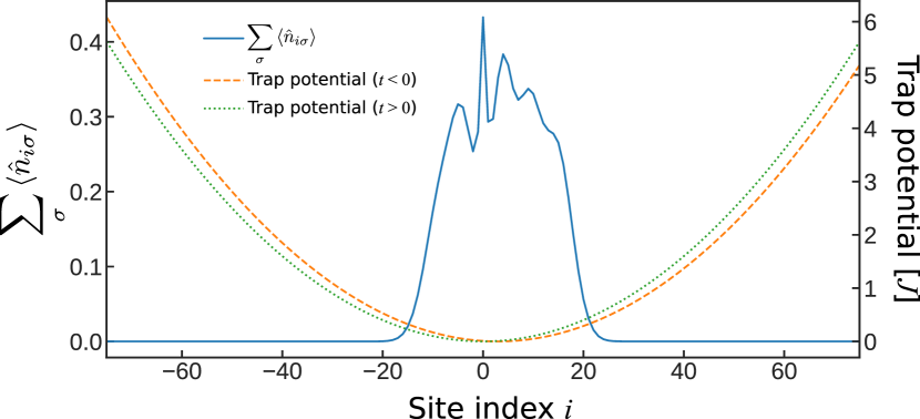
Figure 1: (Color online) The solid line represents the density distribution of the delocalized fermions of the Kondo model in the stationary state for $N=9$, total magnetization $M=0$, $V/J=1$, $x_{c}=3a$, and $\beta J=75$. The localized fermion is located at $i=0$. The dashed and dotted lines represent the parabolic trap potential before and after the displacement of its center.

In order to numerically simulate dynamics of quantum many-body systems at finite temperatures, we use MPS and the METTS algorithm. There is another option for computing such finite-temperature dynamics, namely, the purification method Verstraete et al. (2004); Feiguin and White (2005); Binder and Barthel (2015); Goto and Danshita (2017). However, since in the purification method the density matrix of a system is represented as a pure state by squaring the dimensions of local Hilbert spaces, it is not very efficient for our two-orbital system with large local Hilbert spaces.

In the METTS algorithm, thermal expectation value at an inverse temperature $\beta=1/k_{\mathrm{B}}T$ is calculated as

$$\braket{\hat{O}}_{\mathrm{\beta}} =\frac{\mathrm{Tr}\left[\mathrm{e}^{-\frac{\beta}{2}\hat{H}}\hat{O}\mathrm{e}^{-\frac{\beta}{2}\hat{H}}\right]}{Z}$$ (2)

$$=\sum_{i}\frac{\Braket{i}{\mathrm{e}^{-\beta\hat{H}}}{i}}{Z}\frac{\Braket{i}{\mathrm{e}^{-\frac{\beta}{2}\hat{H}}\hat{O}\mathrm{e}^{-\frac{\beta}{2}\hat{H}}}{i}}{\Braket{i}{\mathrm{e}^{-\beta\hat{H}}}{i}},$$

and the summation over orthonormal basis $\ket{i}$ is performed by the Markov-chain Monte Carlo (MCMC) sampling. In the ordinary METTS algorithm White (2009); Stoudenmire and White (2010), the transition probability of MCMC method from a state $\ket{i}$ to $\ket{j}$ is given by

$$p_{i\to j}=\frac{\left|\Braket{j}{\mathrm{e}^{-\frac{\beta}{2}\hat{H}}}{i}\right|^{2}}{\Braket{i}{\mathrm{e}^{-\beta\hat{H}}}{i}}$$ (3)

With this transition probability, the METTS algorithm suffers from a severe autocorrelation problem at high temperatures as easily inferred from the $\beta\to 0$ limit. This autocorrelation problem can be eliminated by breaking the total particle number conservation. However, the breaking of the conservation of particle number leads to significant increase of computation time in dynamics. Hence, we introduce the following transition probabilities for odd steps,

$$p^{\mathrm{odd}}_{i\to j}=\frac{\left|\Braket{j}{{\left[\hat{U}(\tau)\right]}^{n}\mathrm{e}^{-\frac{\beta}{2}\hat{H}}}{i}\right|^{2}}{\Braket{i}{\mathrm{e}^{-\beta\hat{H}}}{i}}$$ (4)

and

$$p^{\mathrm{even}}_{i\to j}=\frac{\left|\Braket{j}{\mathrm{e}^{-\frac{\beta}{2}\hat{H}}{\left[\hat{U}^{\dagger}(\tau)\right]}^{n}}{i}\right|^{2}}{\Braket{i}{{\left[\hat{U}(\tau)\right]}^{n}\mathrm{e}^{-\beta\hat{H}}{\left[\hat{U}^{\dagger}(\tau)\right]}^{n}}{i}}$$ (5)

for even steps. Here, $\tau$ is a parameter which characterizes the Trotter gates,

$$\hat{U}(\tau)=\mathrm{e}^{-\mathrm{i}\tau\hat{H}_{\mathrm{even}}}\mathrm{e}^{-\mathrm{i}\tau\hat{H}_{\mathrm{odd}}},$$ (6)

and $n$ is an integer. For $\hat{H}_{\mathrm{even}}$ and $\hat{H}_{\mathrm{odd}}$, one can take any hermitian operators as long as they respect the conservation of particle number. We use the products of local Hilbert states in some symmetric sector as the orthonormal basis $\ket{i}$. This approach is a variant of the symmetric METTS algorithm Binder and Barthel (2017) with symmetric bases $\ket{i}$ and ${\left[\hat{U}^{\dagger}(\tau)\right]}^{n}\ket{i}$, which are very flexible because of the parameter $\tau$ and the freedom to choose $\hat{H}_{\mathrm{even}}$ and $\hat{H}_{\mathrm{odd}}$. Moreover, the implementation of our approach is quite easy since it requires only the applications of the Trotter gates in addition to the ordinary METTS algorithm. With the transition probabilities, we can reduce the autocorrelation time by increasing $\tau$ and $n$ without breaking the conservation. However, since the bond dimensions of MPS increase with $\tau$ and $n$, some tuning of the parameters may be required for efficient simulations. The validity of our approach and some benchmark results are shown in Supplemental Material .

The dynamics of thermal expectation value is obtained by representing the operator $\hat{O}$ in the Heisenberg picture $\hat{O}(t)=\mathrm{e}^{\mathrm{i}t\hat{H}^{\prime}/\hbar}\hat{O}\mathrm{e}^{-\mathrm{i}t\hat{H}^{\prime}/\hbar}$ with the Hamiltonian $\hat{H}^{\prime}$ after a quench. Both imaginary and real time evolutions of MPS in this study are performed with the time-evolving block decimation method Vidal (2003, 2004); White and Feiguin (2004); Daley et al. (2004) using the optimized Forest-Ruth-like decomposition Omelyan et al. (2002). Throughout this study, we set $w/J=0.001$, the number of delocalized fermions $N$ to nine, $L=75$, $\tau=1.0/J$, $n=4$, and $\hat{H}_{\mathrm{even}}$ ($\hat{H}_{\mathrm{odd}}$) is the Hamiltonian linking even (odd) bonds of the Kondo model (1). On-site terms are equally divided to $\hat{H}_{\mathrm{even}}$ and $\hat{H}_{\mathrm{odd}}$. Truncation error is set to $10^{-10}$ in imaginary-time evolution and $10^{-8}$ in real-time evolution, and the bond dimensions are allowed to increase up to $4000$.

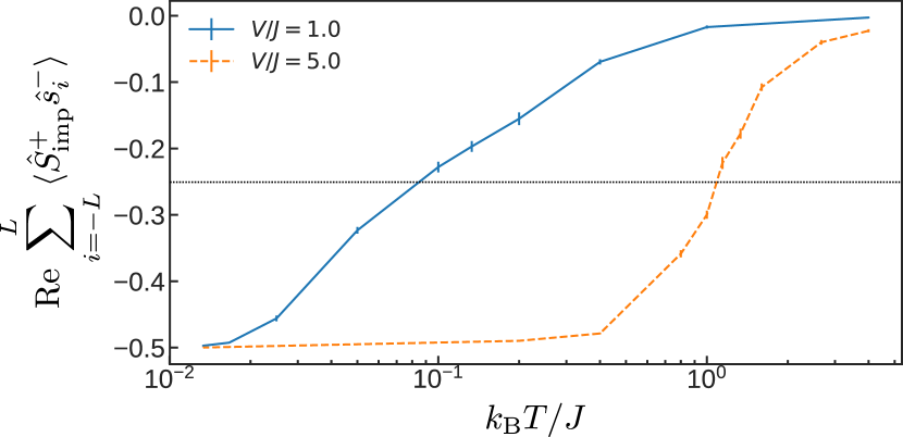
Figure 2: (Color online) The spin correlation versus temperature in steady states for $V/J=1$ (blue solid line) and $5$ (orange dashed line). Error bars indicate 1$\sigma$ uncertainty. The horizontal dotted line represents $\mathrm{Re}\sum_{i}\braket{\hat{S}^{+}_{\mathrm{imp}}\hat{s}^{-}_{i}}=-0.25$, the criterion we used to define the Kondo temperature. We set $M=0$ and $x_{\mathrm{c}}=0$.

Antiferromagnetic case.— We first consider the case that the spin exchange interaction is antiferromagnetic and the total magnetization is zero, i.e., $V>0$ and $M=\Braket{\hat{S}^{z}_{\mathrm{imp}}+\sum_{i}\hat{s}^{z}_{i}}=0$. In order to identify a temperature range in which the Kondo effect occurs, we show in Fig. 2 the spin correlation, $\mathrm{Re}\sum_{i}\braket{\hat{S}^{+}_{\mathrm{imp}}\hat{s}^{-}_{i}}=\sum_{i}\braket{\hat{S}^{x}_{\mathrm{imp}}\hat{s}^{x}_{i}+\hat{S}^{y}_{\mathrm{imp}}\hat{s}^{y}_{i}}$, for $V/J=1$ (blue solid line) and $5$ (orange dashed line), as a function of the temperature. It is clearly seen that when the temperature decreases, the spin correlation grows logarithmically, implying the formation of a many-body spin-singlet.

From these spin correlations, we can extract an important energy scale called Kondo temperature $T_{\mathrm{K}}$. At $T\lesssim T_{\mathrm{K}}$ the spin-singlet correlation grows such that it makes significant contributions to physical quantities. In this study, we define the Kondo temperature as a temperature at the spin correlation $\mathrm{Re}\sum_{i}\braket{\hat{S}^{+}_{\mathrm{imp}}\hat{s}_{i}}$ becomes $-0.25$, namely the half of the maximal singlet value. As discussed in Supplemental Material Note (1), the Kondo temperatures given by this definition behave similarly to the ordinary Kondo temperatures obtained by the perturbative renormalization group analysis Hewson (1997) at least around $V/J=1$. The Kondo temperature at $V/J=1$ is around $0.1J/k_{\mathrm{B}}$ and the estimated size of the Kondo screening cloud is around $10a$ Note (1); Sørensen and Affleck (1996). In the following calculations for real-time dynamics at $V/J=1$, we take $7.5\leq\beta J\leq 75.0$, which corresponds approximately to $0.1\leq T/T_{\mathrm{K}}\leq 1$. Moreover, itinerant atoms are distributed over 40 sites (See Fig. 1), which is sufficiently larger than the Kondo screening length. Thus, our setting is adequate for observing the Kondo physics.

Notice that the Kondo temperature $T_{\mathrm{K}}\sim 0.1J/k_{\mathrm{B}}$ at $V/J$ is remarkably lower than the lowest temperature, $T=0.25J/k_{\rm B}$, achieved in experiments with ultracold fermions Mazurenko et al. (2017). We emphasize that the Kondo temperature can be significantly lifted by increasing $V/J$. For instance, Fig. 2 shows that $T_{\mathrm{K}}$ at $V/J=5$ is well above $T=0.25J/k_{\rm B}$. Nevertheless, we set $V/J=1$ for computations of real-time dynamics because the numerical cost is much more expensive for higher temperatures.

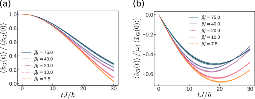
Figure 3: (Color online) Time evolution of the normalized COM positions (a) and velocities (b) for several temperatures. We set $V/J=1$ and $M=0$. The shaded regions are 1$\sigma$ uncertainty of trajectories.

Figure 3 shows the time evolution of the COM positions and velocities at several temperatures after the shift of the trap center from $x_{\mathrm{c}}=3a$ to $x_{\mathrm{c}}=0$. The COM positions and velocities are respectively normalized by $\braket{\hat{x}_{\rm G}(0)}$ and $\omega_{\rm f}\braket{\hat{x}_{\rm G}(0)}$, where $\omega_{\rm f}=2\sqrt{wJ}/\hbar$ denotes the dipole oscillation frequency of free particles Rey (2004). $\omega_{\rm f}\braket{\hat{x}_{\rm G}(0)}$ means the maximum speed during the undamped dipole oscillation starting with the position $\braket{\hat{x}_{\rm G}(0)}$. In Fig. 3, we see that the transport is significantly suppressed when the temperature decreases. This tendency is reminiscent of the Kondo effect, in which the resistance increases with decreasing the temperature.

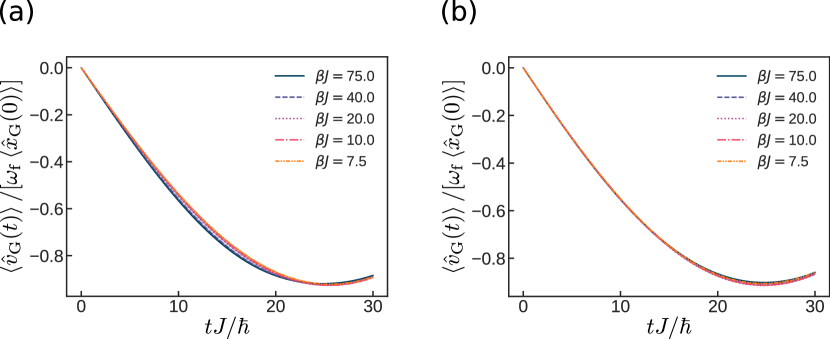
Figure 4: (Color online) Time evolution of the normalized COM velocities in the fully spin-polarized system with $V/J=1$ (a) and in the ferromagnetic Kondo model with $V/J=-1$ (b). 

Fully spin-polarized and ferromagnetic cases.— In order to support our argument that the suppression of transport is a manifestation of the Kondo effect, we also compute the quench dynamics of the following two systems, which are widely known NOT to exhibit the Kondo effect Furusaki (2005). The first example is a fully spin-polarized system ($M=5$), in which the spin-exchange interaction term in Eq. (1) acts as a simple potential barrier term. In this system, we completely prohibit spin-flip processes that are essential for the Kondo effect Kondo (1964). Figure 4 (a) represents the dynamics of the normalized COM velocities in the fully spin-polarized system. Except the total magnetization $M$, any other settings are equivalent to those of the dynamics shown in Fig. 3. In contrast to the $M=0$ case in Fig. 3 (b), the normalized velocities in Fig. 4 (a) does not show visible temperature dependence. This behavior is consistent with the formula of the resistance, $R\propto T^{2K-2}$, obtained from the Tomonaga-Luttinger (TL) liquid theory, where $K$ denotes the Luttinger parameter for the charge sector and $K=1$ for noninteracting fermions Kane and Fisher (1992); Kagan et al. (2000); Büchler et al. (2001); Danshita (2013).

The second example is the case that the spin-exchange interaction is ferromagnetic. Specifically, we take $V/J=-1$ and $M=0$. Notice that while there exists the ferromagnetic Kondo effect in 1D for $K<1$ Furusaki and Nagaosa (1994); Furusaki (2005), this is not the case for non-interacting delocalized fermions considered here. This happens because they are also described by the TL liquid theory with $K=1$. Figure 4 (b) shows the time dependence of the normalized COM velocities in the ferromagnetic Kondo model. Except the sign of $V/J$, any other settings are equivalent to the settings in Fig. 3. Likewise the fully spin-polarized case, the normalized COM velocities in the ferromagnetic Kondo model do not exhibit visible temperature dependence and this is also consistent with $R\propto T^{2K-2}$.

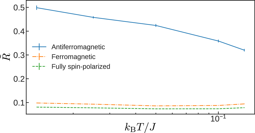
Figure 5: (Color online) Temperature dependence of $\tilde{R}=1-\max_{t}|\langle\hat{v}_{\rm G}(t)\rangle|/(\omega_{\rm f}\langle\hat{x}_{\rm G}(0)\rangle)$. The solid, dashed, dashed-dotted lines represent the antiferromagnetic Kondo ($M=0$ and $V/J=1$), fully spin-polarized ($M=5$ and $V/J=1$), and ferromagnetic Kondo ($M=0$ and $V/J=-1$) systems. Error bars indicate 1$\sigma$ uncertainty. 

In order to discuss the temperature dependence of the transport more quantitatively, we plot the quantity, $\tilde{R}=1-\max_{t}|\braket{\hat{v}_{\rm G}(t)}|/[\omega_{\rm f}\braket{\hat{x}_{\rm G}(0)}]$, in Fig. 5. As shown in the Supplemental Material Note (1), $\tilde{R}$ is approximately proportional to the resistance $R$ under the assumption that $\tilde{R}\ll 1$, and is suited to characterizing the transport. In Fig. 5, we see that the temperature dependence of the transport is only visible in the antiferromagnetic Kondo model with spin-flip processes (blue solid line). We emphasize that the horizontal axis of Fig. 5 is logarithmic scale; $\tilde{R}$ of the antiferromagnetic Kondo model exhibits a logarithmic growth with decreasing the temperature, which is a characteristic feature of the Kondo effect. Specifically, the “resistance” $\tilde{R}$ increases by around 1.7 times when the temperature decreases from $T\sim T_{\mathrm{K}}$ to $0.1T_{\mathrm{K}}$. Strictly speaking, we observe only the lower temperature side $0.1\lesssim T/T_{\mathrm{K}}\lesssim 1$ of the expected logarithmic dependence Costi (2000); Merker et al. (2013). For the higher temperature side $1\lesssim T/T_{\mathrm{K}}\lesssim 10$, it requires very expensive numerical cost. In this sense, corroborating the logarithmic dependence in the higher temperature region will be a suitable target of OLQS experiments. We suggest that observation of the logarithmic temperature dependence serves as a smoking-gun signature of the Kondo effect in the OLQS of the Kondo model.

Summary.— In order to propose an experimental way for observing the Kondo effect with ultracold alkaline-earth-like atoms in optical lattices, we numerically simulated the finite temperature dynamics of the one-dimensional Kondo model with using quasi-exact minimally entangled typical thermal states (METTS) algorithm based on matrix product states. We found that when the spin-exchange interaction is antiferromagnetic, the COM motion after a sudden displacement of the trap potential is suppressed logarithmically with decreasing the temperature. In contrast, it was shown that such suppression of the transport is absent in the ferromagnetic Kondo model or the fully spin-polarized system. These findings convincingly indicate that the Kondo effects in ultracold atoms are detectable via the simple transport measurement.

We also improved the numerical efficiency of the METTS algorithm without breaking the total particle number conservation by the applications of the Trotter gates. The modified METTS algorithm can be applied to other systems for accurately analyzing static and dynamical properties at finite temperatures, such as the spectral functions Coira et al. (2018) and the out-of-time ordered correlations Bohrdt et al. (2017).