Intrinsic Weight Learning Approach for Multi-view Clustering

Abstract

Exploiting different representations, or views, of the same object for better clustering has become very popular these days, which is conventionally called multi-view clustering. Generally, it is essential to measure the importance of each individual view, due to some noises, or inherent capacities in description. Many previous works model the view importance as weight, which is simple but effective empirically. In this paper, instead of following the traditional thoughts, we propose a new weight learning paradigm in context of multi-view clustering in virtue of the idea of re-weighted approach, and we theoretically analyze its working mechanism. Meanwhile, as a carefully achieved example, all of the views are connected by exploring a unified Laplacian rank constrained graph, which will be a representative method to compare with other weight learning approaches in experiments. Furthermore, the proposed weight learning strategy is much suitable for multi-view data, and it can be naturally integrated with many existing clustering learners. According to the numerical experiments, the proposed intrinsic weight learning approach is proved effective and practical to use in multi-view clustering.

1 Introduction

Many practical applications involve data obtained from multiple sources or collected with various extractors, usually known as views. Although each individual view can be directly used for any specific task, they are expected to work better when appropriately combined. Therefore, how to effectively cluster such kind of data has become a very hot topic.

Straightforwardly, one can choose to fuse multiple views into a single one (e.g., concatenation) in feature space and input it to a typical clustering algorithm, such as $k$-means or its kernel version [1], spectral clustering [2], affinity propagation [3], etc. However, this approach is not physically meaningful and prone to cause overfitting in the case of a small size training sample [4]. Multi-view clustering methods often model each particular view respectively and jointly optimize them to obtain the final clustering result. In most cases, they balance the the view efficiency and the view disagreement due to a potential assumption that multiple views are complementary as well as consistent [4, 5].

There are quantities of previous works that focus on clustering data with multiple representations in the last two decades. The co-training based multi-view clustering methods [6, 7, 8, 9] can be seen as the extension from the co-training classification to clustering context. The basic idea of this series works is that the views are on equal terms and they can teach each other. Therefore, the clustering results of different views may be inconsistent. For instance, even with the employed regularization, in [8], the authors suggest randomly selecting a view when the disagreement arises. For handy multiple views, to avert the aforementioned trouble, an intuitive way is to learn a unified representation after optimization. According to the literature, this thought is extensively achieved in graph-based clustering, such as joint matrix factorization approaches [10, 11, 12], graph integration [13, 14, 15], the CCA(canonical correlation analysis)-based [16, 17]. These methods succeed by exploiting a shared data structure which can better encode the relationships among the instances.

Actually, how to model the view importance is essential in multi-view clustering (or even in all of multi-view learning tasks). It is due to the fact that view variance widely exists in real multi-view data. There are two common conditions: 1) some views are corrupted by noise in different degree while others are clean; 2) some views are instinctively less powerful in description than others (E.g., color moments is to HOG (Histograms of Oriented Gradients) [18] in the family of image features). Many works model the view importance as weight and applies it on the clustering model level, which is very simple but effective. Therefore, different weight learning strategies have been developed these years, but all of them follow the same route that the view weight is explicitly defined in the objective and then it is optimized as a target variable. However, in this paper, we propose a new weight learning approach which naturally matches the multi-view clustering and significantly improves the clustering performance. What’s more, it is usually compact and light in form. Besides applying this weight learning approach in some recent clustering learners, we present that it is easily extended to more clustering method to multi-view context. The major contributions of this work are summarized as followings:

1. We propose a general intrinsic weight learning approach for multi-view clustering, whose working mechanism, convergence, and time complexity are carefully discussed in the paper.

2. Apart from theoretical comparison among different weight learning strategies for multi-view clustering, we achieve them in an identical base clustering learner and then their final clustering performances and learned weights are investigated in experiments.

3. We present that the proposed weight learning approach is easily integrated into more clustering methods, whose performances significantly outperform the baselines.

The rest of the paper is organized as follows: Section 2 revisits some previous methods that handle the view variance in different ways, in which we systematically summarize several representative automatical weight learning methods. In Sections 3 and 4, we describe the details of intrinsic weight learning approach and the relative theoretical analysis. Then we achieve an important example in Section 5, which combines the proposed weight learning approach with a recent graph-based clustering learner. Section 6 conducts numerous experiments to evaluate the proposed approach. Finally, Section 7 concludes this paper.

2 Related works

Many previous multi-view clustering methods have made attempts to address the view variance problem. In [9], the authors points out that learning the view importance is very necessary, but they simply resort to the extra prior knowledge in the paper. Some others, such as recent approaches [19, 20], tackle this problem by modeling the separated noise in each view and learn a shared clean data structure. However, this way is not able to cover the second case of view variance because of the gap of real noises and clustering errors by a weak view. As a matter of fact, measuring the view importance with the weight is direct and useful, and many works prefer this way. For convenience, [21] proposes to roughly compute the weights according to the proportion of the graph volume in each view. Obviously, this strategy is manually intervening and much shallow. Practically, most works would prefer to learn the weights automatically or adaptively. That means they usually optimize the objective and weights simultaneously. In the followings, we particularly introduce several types of how the previous works learn the weights which is closely related our work.

Suppose the clustering method for $i$-th view can be reduced to the minimization of the following objective function

$$\mathop{\min}\limits_{{x_{c}}\in{\mathcal{C}_{c}},{x_{s}}\in{\mathcal{C}_{s}}}\Phi_{i}\left({{x_{c}},{x_{s}}}\right),$$ (1)

where $x_{c},x_{s}$ denote the set of view-common variables and view-specific variables, $\mathcal{C}_{c},\mathcal{C}_{s}$ are the proxy constraints to $x_{c}$ and $x_{s}$ respectively. Noting that each view is coupled by $x_{c}$, for ease of notation, we instead adopt $x$ (Formally, let $x\in\mathcal{C}_{x}$) to represent the view-common variables and ignore the view-specific variables. Given a total of $M$ available views, one can derive a weighted multi-view clustering objective by minimizing a linear combination form of

$$\mathop{\min}\limits_{x,\alpha}\sum\limits_{v=1}^{M}{{\alpha_{v}}{\Phi_{v}}\left(x\right)}\quad s.t.\,\alpha\in\mathcal{C}_{\alpha},x\in\mathcal{C}_{x},$$ (2)

where $\alpha=\left[{{\alpha_{1}},{\alpha_{2}},...,{\alpha_{M}}}\right]$, $\mathcal{C}_{\alpha}$ denotes constraints ${\alpha_{v}}\geq 0,\alpha{{\bf{1}}_{M}}=1$ (${{\bf{1}}_{M}}$ is a $M$-dimensional column vector where each element is 1). It can be easily verified that Eq. (2) has the trivial solution: the weight of best view (which has the lowest value of objective in Eq. (1)) is assigned to 1 while others are 0s. This result is apparently contrary to the assumption that all of views are usually useful. In this perspective, the following prototypes are all designed for avoiding this over-sparse problem.

1. Norm Regularization (NR)

   To make the weight distribution flater, some works [22, 23, 24, 25] add a norm regularization term, and thus the objective comes to

   $$\mathop{\min}\limits_{x,\alpha}\sum\limits_{v=1}^{M}{{\alpha_{v}}{\Phi_{v}}\left(x\right)}{\rm{+}}\gamma_{1}\left\|\alpha\right\|_{2}^{2}\quad\,\,s.t.\,\alpha\in\mathcal{C}_{\alpha},x\in\mathcal{C}_{x},$$ (3)

   where $\gamma_{1}$ is a non-negative parameter which controls the degree of flatness. When $\gamma_{1}\to 0$, Eq. (3) reduces to Eq. (2) and the best view will be selected. On the contrary, when $\gamma_{1}\to\infty$, the equal weights will be obtained. Particularly, when $x$ is fixed, the derived subproblem is

   $$\mathop{\min}\limits_{\alpha}\left\|{\frac{\phi}{{2\gamma_{1}}}+\alpha}\right\|_{2}^{2}\quad s.t.\,\alpha\in{\mathcal{C}_{\alpha}},$$ (4)

   where $\phi=\left[{{\Phi_{1}}\left(x\right),{\Phi_{2}}\left(x\right),...,{\Phi_{M}}\left(x\right)}\right]$. This problem can be effectively solved by the algorithm in [26], and the obtained weights are usually sparse (see the discussion therein.).

2. Entropy Regularization (ER).

   An alternative to NR is to utilize the maximum entropy [27] to penalize the weights. It can be described as

   $$\mathop{\min}\limits_{x,\alpha}\sum\limits_{v=1}^{M}{\big{(}{\alpha_{v}}{\Phi_{v}}\left(x\right){\rm{+}}\gamma_{2}{\alpha_{v}}\log{\alpha_{v}}\big{)}}\quad s.t.\,\alpha\in{\mathcal{C}_{\alpha}},x\in{\mathcal{C}_{x}},$$ (5)

   where $\gamma_{2}$ has the identical effect with $\gamma_{1}$ in Eq. (3). Many previous works learn the weights in this way, such as [28, 29]. Similarly, when $x$ is fixed, we give the analytical solution to the corresponding subproblem as

   $${\alpha_{v}}=\frac{{\exp\left({{{\left({-{\gamma_{2}}-{\Phi_{v}}\left(x\right)}\right)}\mathord{\left/{\vphantom{{\left({-{\gamma_{2}}-{\Phi_{v}}\left(x\right)}\right)}{{\gamma_{2}}}}}\right.\kern-1.2pt}{{\gamma_{2}}}}}\right)}}{{\sum\limits_{u=1}^{M}{\exp\left({{{\left({-{\gamma_{2}}-{\Phi_{u}}\left(x\right)}\right)}\mathord{\left/{\vphantom{{\left({-{\gamma_{2}}-{\Phi_{j}}\left(x\right)}\right)}{{\gamma_{2}}}}}\right.\kern-1.2pt}{{\gamma_{2}}}}}\right)}}}\quad\forall 1\leq v\leq M,$$ (6)

   which is also known as Gibbs distribution as in [28]. According to Eq. (6), it can be observed that when ${{{\Phi_{v}}\left(x\right)}\mathord{\left/{\vphantom{{{\Phi_{i}}\left(x\right)}{{\gamma_{2}}}}}\right.\kern-1.2pt}{{\gamma_{2}}}}$ is very large, $\alpha$ will be very small. Thus, loosely speaking, this strategy also learns the sparse weights.

3. Exponent Flattening (EF).

   Another approach to smoothen the weight distribution is to introduce a parameter as the exponent of each $\alpha_{i}$

   $$\mathop{\min}\limits_{x,\alpha}\sum\limits_{v=1}^{M}{\alpha_{v}^{{\gamma_{3}}}{\Phi_{v}}\left(x\right)}\quad s.t.\,\alpha\in{\mathcal{C}_{\alpha}},x\in{\mathcal{C}_{x}},$$ (7)

   where ${\gamma_{3}}>1$. Due to the free of the regularization term, numerous multi-view clustering works [30, 31, 23, 29, 32] have adopted it. Fixing $x$, the solution of the subproblem can be given as

   $${\alpha_{v}}={{1\mathord{\left/{\vphantom{1{\sum\limits_{u=1}^{M}{\left({\frac{{{\Phi_{v}}\left(x\right)}}{{{\Phi_{u}}\left(x\right)}}}\right)}}}}\right.\kern-1.2pt}{\sum\limits_{u=1}^{M}{\left({\frac{{{\Phi_{v}}\left(x\right)}}{{{\Phi_{u}}\left(x\right)}}}\right)}}}^{\frac{1}{{{\gamma_{3}}-1}}}}\quad\forall 1\leq v\leq M.$$ (8)

3 Intrinsic Weight Learning Approach

Figure 1: (a): When $0<p\leq 2$, how $\Phi_{v}^{p/2}$ varies with the change of $\Phi_{v}$. (b) The weight $\alpha_{v}$ as a function of $\Phi_{v}$ and $p$.

It is observed that previous works learn the weights by introducing a view-specific weight factor for each view in the objective, then utilizing a hyper-parameter to constrain the weight distribution, and finally solving the weights as the target variables. However, empirical studies show that they are usually sensitive to the value of the hyper-parameter (we also verify this idea in our experiments). More importantly, these methods do not touch the multi-view weights in essence because they fail to dig out the view relation according to view efficiency. To alleviate above problems, we propose a novel intrinsic weight learning approach for multi-view clustering, whose objective is

$$\mathop{\min}\limits_{x}\sum\limits_{v=1}^{M}{\Phi_{v}^{\frac{p}{2}}\left(x\right)}\quad s.t.\,x\in{\mathcal{C}_{x}},$$ (9)

where $p$ satisfies $0<p\leq 2$. At the first sight, there is no weight explicitly defined in the objective, but we will see how this formulation learns intrinsic weights.

Let $\mathcal{G}(\Lambda,x)$ serve as the proxy of the constraints to $x$, and then the Lagrange function of Eq. (9) is

$$\mathop{\min}\limits_{x}\sum\limits_{v=1}^{M}{\Phi_{v}^{\frac{p}{2}}(x)}+\mathcal{G}\left(\Lambda,x\right),$$ (10)

where $\Lambda$ represents the Lagrange multiplier. Taking the derivative of Eq. (10) w.r.t $x$ and setting the derivative to zero, we have

$$\sum\limits_{v=1}^{M}{{\alpha_{v}}\frac{{\partial{\Phi_{v}}(x)}}{{\partial x}}}+\frac{{\partial\mathcal{G}\left({\Lambda,x}\right)}}{{\partial x}}=0,$$ (11)

where

$${\alpha_{v}}=\frac{p}{2}\Phi_{v}^{\frac{{p-2}}{2}}\left(x\right)\quad\forall 1\leq i\leq M.$$ (12)

Since the factors of the first term in Eq. (11) are coupled with each other, Eq. (11) cannot be directly solved. However, if $\alpha_{v}$ is fixed, then the solution of Eq. (11) is equal to solving a linearly combined multi-view clustering problem

$$\mathop{\min}\limits_{x}\sum\limits_{v=1}^{M}{{\alpha_{v}}{\Phi_{v}}(x)}\quad s.t.\,x\in{\mathcal{C}_{x}}.$$ (13)

This problem is easier to handle. Particularly, if ${\Phi_{v}}(x)$ is linear w.r.t $x$, Eq. (13) will be reduced to a single clustering model but with the fused feature as the input. Then, the calculated variable $x$ can be further used to update $\alpha_{v}$, which inspires us to solve the problem (9) by alternatively optimizing $x$ and $\alpha_{v}$ iteratively. Once this procedure converges, we find that Eq. (13) is the exact form what need to be learned, and the corresponding weights are naturally obtained. In other words, solving a general problem as Eq. (9), where the weights are not explicitly defined in the objective, actually induces a weighted linear combination of clustering models for different views. To distinguish with the aforementioned traditional weights learning methods, we call this multi-view weight learning strategy as Intrinsic Weight (IW) learning approach, which is summarized into Algorithm 1.

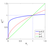
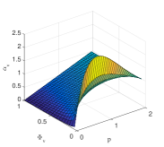
In Fig. 1(a), we present how the view clustering function value changes with the different powers (For ease of description, we use $\Phi_{v}$ as a variable when referring to $\Phi_{v}(x)$). When $p=2$, Eq. (9) is equal to average weight learning. When $p$ becomes smaller, the different $\Phi_{v}$ will be amplified in different degrees. In one-step optimization, the weight $\alpha_{v}$ is computed by Eq. (12), which is drawn into Fig. 1(b), where $\Phi_{v}$ is normalized to 0-1 range. Then this approach have the following properties:

(1) For $0<p\leq 2$, a view which has the smaller value of $\Phi_{v}$ will be assigned to a larger weight, and vice versa.

For Eq. (12), taking the partial derivative of $\alpha_{v}$ w.r.t $\Phi_{v}$, we obtain that

$$\frac{{\partial{\alpha_{v}}}}{{\partial{\Phi_{v}}}}=\frac{{p\left({p-2}\right)}}{4}\Phi_{v}^{\frac{{p-4}}{2}}\leq 0$$

holds for $0<p\leq 2$. It means that once $p$ is fixed, with the increasing of $\Phi_{v}$, $\alpha_{v}$ will be monotonically decreasing. This agrees with our knowledge, and guarantees the meaning of weights.

(2) The hyper-parameter $p$ control the smoothness of the learned weight distribution.

Obviously, when $p=2$, we come to the equal weights version. Now, we consider the conditions when $0<p<2$. Let ${\alpha_{v}}=f\left({p,{\Phi_{v}}}\right)=\frac{p}{2}\Phi_{v}^{\frac{{p-2}}{2}}$, ${\phi_{\max}}=\max\left\{{{\Phi_{v}}}\right\}_{v=1}^{M}=1$, and ${\phi_{\min}}=\min\left\{{{\Phi_{v}}}\right\}_{v=1}^{M}$, then the sharpest weight distribution can be approximately derived by choosing $p$ which is determined by

$$p=\mathop{\arg\max}\limits_{p}\left({f\left({p,{\phi_{\min}}}\right)-f\left({p,{\phi_{\max}}}\right)}\right).$$

Since $f\left({p,1}\right)=\frac{p}{2}\in\left({0,1}\right)$ and ${\left.{f\left({p,{\phi_{\min}}}\right)}\right|_{{\phi_{\min}}\to 0}}=\infty$, it can be concluded that ${{\phi_{\min}}}$ plays the dominant role in choosing the hyper-parameter $p$. Taking the partial derivative of $\alpha_{v}$ w.r.t $p$, and setting the derivative to zero, we obtain

$${\left.{\frac{{\partial{\alpha_{v}}}}{{\partial p}}}\right|_{{\Phi_{v}}={\phi_{\min}}}}={\phi_{\min}}^{\frac{{p-2}}{2}}\left({1+\frac{p}{2}\ln{\phi_{\min}}}\right)=0.$$

Thus, roughly speaking, we obtain the sharpest weight distribution when $p=\frac{{-2}}{{\ln{\phi_{\min}}}}$ .

Algorithm 1 Intrinsic weight learning approach to solve a general problem as Eq. (9)

0:  Hyperparameter $p$, other parameters needed for solving problem (1).Initialize the weight for each view (e.g., $\alpha_{v}=\frac{1}{M}$).

  repeat

     1. Calculate $x$ by solving Eq. (13).

     2. Update $\alpha_{v}$ by using Eq. (12).

  until converge

  $x$ used for clustering, $\alpha_{v}$ for each view.

(3) The proposed approach learns the weights by passing the information through view-common variables.

In each iteration in Algorithm 1, given the value of $p$, it is noted from Eq. (12) that the weight $\alpha_{i}$ only relies on $\Phi_{v}$. However, according to Eq. (13), we find any $\Phi_{j}$ $(j\neq i)$ and $\alpha_{i}$ are correlated by the view-common variables, which is quite different from traditional weight learning approaches (see Eqs. (4), (6), and (8)). In other words, the aforementioned weight learning approaches are not specialized for multi-view learning, such as [24], while this intrinsic weight learning approach is digging out the actual view relation under the view coupling assumption.

The most related works about this weight learning paradigm is re-weighed theories [33, 34, 35]. [33] firstly propose the re-weight approach to solve the linear least maximum approximation problem. Later, this idea is successfully applied in compressive sensing [36], sparse recovery [37], and robust feature selection [38], etc. Different from the original re-weight theory, where the weight is employed to each single instance, [35] extends the re-weight approach to a more general sense, i.e., utilizing the supergradients of concave functions to iteratively re-weight the concave functions. In this paper, we introduce re-weight approach into multi-view learning, but the key point stressed here is to provide a compact form to learn the view weights in multi-view clustering and demonstrate the weights efficiency.

4 Theory Analysis

This section presents the analysis of intrinsic weight learning approach in two aspects. We first prove the convergence of Algorithm 1, and then analyze its time complexity.

4.1 Convergence

In this part, we prove that alternatively update $x$ and $\alpha_{v}$ in Algorithm 1 will monotonically decrease the objective of Eq. (9) in each iteration. First, we introduce the following lemma.

Lemma 1: When $0<p\leq 2$, for any positive number $u$ and $v$, the following inequality holds:

$${u^{p}}-\frac{p}{2}\frac{{{u^{2}}}}{{{v^{2-p}}}}\leq{v^{p}}-\frac{p}{2}\frac{{{v^{2}}}}{{{v^{2-p}}}}.$$ (14)

Proof: Let $h\left(t\right)={t^{p}}-\frac{p}{2}{t^{2}}+\frac{p}{2}-1$, then we have.

$${h^{{}^{\prime}}}\left(t\right)=p{t^{p-1}}-pt=pt\left({{t^{p-2}}-1}\right).$$

It is apparent that when $t>0$ and $0<p\leq 2$, $t=1$ is the only zero point of ${h^{{}^{\prime}}}\left(t\right)$. Seeing that ${h^{{}^{\prime}}}\left(t\right)>0$ $(0<t<1)$ and ${h^{{}^{\prime}}}\left(t\right)<0$ $\left({t>1}\right)$, $t=1$ is the maximum point. Since $h(1)=0$, when $t>0$ and $0<p\leq 2$, $h(t)\leq 0$. Therefore, let ${t^{*}}={u\mathord{\left/{\vphantom{uv}}\right.\kern-1.2pt}v}$ in $h(t)$, then $h({u\mathord{\left/{\vphantom{uv}}\right.\kern-1.2pt}v})\leq 0$. That is to say

$${\left({\frac{u}{v}}\right)^{p}}-\frac{p}{2}{\left({\frac{u}{v}}\right)^{2}}+\frac{p}{2}-1\leq 0.$$

After a transposition, we arrive at Eq. (14). $\Box$

Theorem 1: When $0<p\leq 2$, Algorithm 1 will monotonically decrease the objective in Eq. (9) in each iteration until the convergence.

Proof: In the $k$th iteration

$$\begin{split}{x_{k+1}}&=\mathop{\arg\min}\limits_{x}\sum\limits_{v=1}^{M}{{\alpha_{v}}{\Phi_{v}}\left(x\right)}\\ &=\mathop{\arg\min}\limits_{x}\sum\limits_{v=1}^{M}{\frac{p}{2}\Phi_{v}^{\frac{{p-2}}{2}}\left({{x_{k}}}\right){\Phi_{v}}\left(x\right)},\end{split}$$ (15)

which means

$$\sum\limits_{v=1}^{M}{\frac{p}{2}\Phi_{v}^{\frac{{p-2}}{2}}\left({{x_{k}}}\right){\Phi_{v}}\left({{x_{k+1}}}\right)}\leq\sum\limits_{v=1}^{M}{\frac{p}{2}\Phi_{v}^{\frac{{p-2}}{2}}\left({{x_{k}}}\right){\Phi_{v}}\left({{x_{k}}}\right)}.$$ (16)

Let $u=\Phi_{v}^{\frac{1}{2}}\left({{x_{k+1}}}\right)$ and $v=\Phi_{v}^{\frac{1}{2}}\left({{x_{k}}}\right)$, then according to Lemma 1, we obtain

$$\begin{split}\sum\limits_{v=1}^{M}{\left({\Phi_{v}^{\frac{p}{2}}\left({{x_{k+1}}}\right)-\frac{p}{2}\frac{{{\Phi_{v}}\left({{x_{k+1}}}\right)}}{{\Phi_{v}^{\frac{{2-p}}{2}}\left({{x_{k}}}\right)}}}\right)}\\ \leq\sum\limits_{v=1}^{M}{\left({\Phi_{v}^{\frac{p}{2}}\left({{x_{k}}}\right)-\frac{p}{2}\frac{{{\Phi_{v}}\left({{x_{k}}}\right)}}{{\Phi_{v}^{\frac{{2-p}}{2}}\left({{x_{k}}}\right)}}}\right)}.\end{split}$$ (17)

Summing Eq. (16) and Eq. (17) in both two sides, we arrive at

$$\sum\limits_{v=1}^{M}{\Phi_{v}^{\frac{p}{2}}\left({{x_{k+1}}}\right)}\leq\sum\limits_{v=1}^{M}{\Phi_{v}^{\frac{p}{2}}\left({{x_{k}}}\right)}.$$ (18)

Thus, Algorithm 1 will monotonically decrease the objective of the problem (9) in each iteration. Obviously, since the objective must have a lower bound, the whole procedure will converge. $\Box$

4.2 Time Complexity

Denote the time complexity of solving the subproblem (13) is $\sigma$, then the time complexity of Algorithm 1 is $\mathcal{O}\left({T\left({\sigma+M\varepsilon}\right)}\right)$, where $\varepsilon$ is the time complexity of updating each $\alpha_{v}$ by Eq. (12), and $T$ represents the number of needed iterations. Generally speaking, as $\sigma\gg M\varepsilon$, the total time complexity can be roughly equal to $T\sigma$. Previous work [35] empirically showed the $T$ is no more than 50. Thus, the final time complexity is determined by the employed single clustering model.

5 An Example CLR-IW

In this section, we apply the intrinsic weight learning approach to a recent graph-based clustering method, where the specific details about the whole procedure will be presented. On the one hand, this section presents how to combine a single clustering model with the proposed weight learning strategy. One the other hand, the accomplishment helps to more accurately compare with the traditional weight learning approaches in the experiment part.

5.1 The Base Learner Introduction

Given $N$ samples which can be partitioned into $C$ clusters, graph-based clustering methods usually first construct a similarity matrix to represent the affinities of all the instances. A great number of early works have studied how to design a similarity matrix with high quality, such as [39, 40]. Then, they will be input to graph-based clustering methods, e.g., spectral clustering. Finally, some postprocessings like $k$-means is employed to obtain the discrete clustering results. However, an ideal similarity matrix $S\in\mathbb{R}^{N\times N}$ is supposed to exactly have $c$ connected components, by which way, $S$ is able to be directly used for the clustering task. Recently, [41, 42, 43, 44] have leveraged this prpperty in different ways. We briefly introduce the Constrained Laplacian Rank (CLR) method [44] therein, which is easier to understand and will be the base learner here.

Given an arbitrary input similarity matrix $A\in\mathbb{R}^{N\times N}$, the target similarity matrix can be learned by minimizing the following problem

$$\mathop{\min}\limits_{{s_{i}}{{\bf{1}}_{N}}=1,{s_{ij}}\geq 0,S\in\mathcal{C}}{{\left\|{S-{A}}\right\|}_{F}^{2}},$$ (19)

where $S$ is nonnegative, whose each row sums up to 1, and $\mathcal{C}$ represents the set of $N$ by $N$ square matrices with $C$ connected components. According to the graph theory in [45, 46], the connectivity constraint can be replaced with a rank constraint, and thus Eq. (19) is specified as

$$\mathop{\min}\limits_{{s_{i}}{{\bf{1}}_{N}}=1,{s_{ij}}\geq 0,rank({L_{S}})=N-C}{{\left\|{S-{A}}\right\|}_{F}^{2}},$$ (20)

where $rank(L_{S})$ means the rank of $L_{S}$. The Laplacian matrix $L_{S}=D_{S}-{{\left({{S^{T}}+S}\right)}\mathord{\left/{\vphantom{{\left({{S^{T}}+S}\right)}2}}\right.\kern-1.2pt}2}$, where the degree matrix $D_{S}\in{\mathbb{R}^{N\times N}}$ is defined as a diagonal matrix whose $i$-th diagonal element is $\sum\nolimits_{j}{{{\left({{s_{ij}}+{s_{ji}}}\right)}\mathord{\left/{\vphantom{{\left({{s_{ij}}+{s_{ji}}}\right)}2}}\right.\kern-1.2pt}2}}$. In this way, once the target similarity matrix is solved and we can directly use it for clustering.

5.2 The Proposed Method

Figure 2: A three-view clustering task example. Given $A^{(1)}$, $A^{(2)}$ and $A^{(3)}$ three input views, the target similarity matrix is supposed to have the minimum of the sum of weighted distance between every input view. Simultaneously, $S$ should be guaranteed to lie in the constraint space.

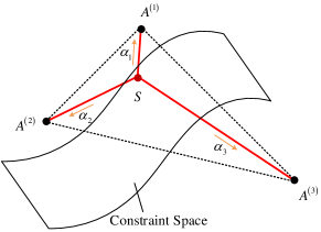
As we stated before, it is useful to assign a weight to each view to measure its importance. Eq. (20) means that the target similarity matrix is expected to be as near as possible to the input one $A$. Therefore, in multi-view context, we expect to learn $S$ to be the centroid of each input $A_{i}$ but with the different confidence for each view. This idea is presented as in Fig. 2. We sum up each single view clustering model with the power of $p$ as indicated in Eq. (9). The objective is written as

$$\mathop{\min}\limits_{{s_{i}}{{\bf{1}}_{N}}=1,{s_{ij}}>0,rank\left({{L_{S}}}\right)=N-C}\sum\limits_{v=1}^{M}{\left\|{S-{A^{\left(v\right)}}}\right\|_{F}^{p}},$$ (21)

where ${{A^{\left(v\right)}}}$ is the $v$-th input similarity matrix, and $0<p\leq 2$. We donate this method as CLR-IW in the following of this paper for better illustration. Following Algorithm 1, we can directly write the two alternative steps of solving the problem (21): solving the following linear combined CLR clustering subproblem

$$\mathop{\min}\limits_{{s_{i}}{{\bf{1}}_{N}}=1,{s_{ij}}>0,rank\left({{L_{S}}}\right)=N-C}\sum\limits_{v=1}^{M}{{\alpha_{v}}\left\|{S-{A^{\left(v\right)}}}\right\|_{F}^{2}},$$ (22)

and updating the $\alpha_{v}$ by

$${\alpha_{v}}=\frac{p}{2}\left\|{S-{A^{\left(v\right)}}}\right\|_{F}^{p-2}.$$ (23)

It is obvious that updating $\alpha_{v}$ is quite simple, while solving the subproblem as Eq. (22) needs further calculations.

To solve Eq. (22), we first let ${\rho_{k}}\left({{L_{S}}}\right)$ to represent $k$-th smallest eigenvalue of $L_{S}$. Seeing that $L_{S}$ is positive semi-definite, ${\rho_{k}}\left({{L_{S}}}\right)>0$. Given a large value of $\lambda$, the rank constraint in Eq. (22) can be eliminated and Eq (22) is equal to the following form

$$\mathop{\min}\limits_{{s_{i}}{{\bf{1}}_{N}}=1,{s_{ij}}>0}\sum\limits_{v=1}^{M}{{\alpha_{v}}\left\|{S-{A^{\left(v\right)}}}\right\|_{F}^{2}}+2\lambda\sum\limits_{k=1}^{C}{{\rho_{k}}\left({{L_{S}}}\right)}$$ (24)

When $\lambda$ is large enough, note that ${\rho_{k}}\left({{L_{S}}}\right)>0$ for each $k$, thus the optimal solution $S$ will make $\sum\limits_{k=1}^{C}{{\rho_{k}}\left({{L_{S}}}\right)}$ to zero and the constraint ${rank\left({{L_{S}}}\right)=N-C}$ will be satisfied. Moreover, according to Ky Fan’s Theory [47], the following equation holds

$$\sum\limits_{k=1}^{C}{{\rho_{k}}\left({{L_{S}}}\right)}=\mathop{\min}\limits_{F\in{R^{N\times C}},{F^{T}}F=I}Tr\left({{F^{T}}{L_{S}}F}\right).$$ (25)

Thus, according to Eq. (25), Eq. (24) is further written to

$$\begin{split}&\mathop{\min}\limits_{S,F}\sum\limits_{v=1}^{M}{{\alpha_{v}}\left\|{S-{A^{\left(v\right)}}}\right\|_{F}^{2}}+2\lambda Tr\left({{F^{T}}{L_{S}}F}\right)\\ &s.t.\,{s_{i}}{{\bf{1}}_{n}}=1,{s_{ij}}>0,F\in{R^{N\times C}},{F^{T}}F=I.\end{split}$$ (26)

We solve this problem by alternatively optimizing variable $F$ and $S$ iteratively as follows.

i. When $S$ is fixed, Eq. (26) becomes

$$\mathop{\min}\limits_{F\in{\mathbb{R}^{N\times C}},{F^{T}}F=I}Tr\left({{F^{T}}{L_{S}}F}\right).$$ (27)

It is known that the optimal solution of $F$ is formed by the $C$ eigenvectors of $L_{S}$ corresponding to the $C$ smallest eigenvalues.

ii. When $F$ is fixed, Eq. (26) can be written as

$$\small\mathop{\min}\limits_{{s_{i}}{{\bf{1}}_{N}}=1,{s_{ij}}\geq 0}\sum\limits_{v=1}^{M}{{\alpha_{v}}\sum\limits_{i,j=1}^{N}{{{\left({{s_{ij}}-a_{ij}^{\left(v\right)}}\right)}^{2}}}}+\lambda\sum\limits_{i,j=1}^{N}{\left\|{{f_{i}}-{f_{j}}}\right\|_{2}^{2}{s_{ij}}}.$$ (28)

Since Eq. (28) is independent for different $i$, we turn to solve the following problem separately for each $i$:

$$\small\mathop{\min}\limits_{{s_{i}}{{\bf{1}}_{N}}=1,{s_{ij}}\geq 0}\sum\limits_{j=1}^{N}{\sum\limits_{v=1}^{M}{{\alpha_{v}}{{\left({{s_{ij}}-a_{ij}^{\left(v\right)}}\right)}^{2}}}}+\lambda\sum\limits_{j=1}^{N}{\left\|{{f_{i}}-{f_{j}}}\right\|_{2}^{2}{s_{ij}}}.$$ (29)

For ease of presentation, we denote ${v_{ij}}=\left\|{{f_{i}}-{f_{j}}}\right\|_{2}^{2}$ and $v_{i}$ is a row vector with $j$-th element equal to $v_{ij}$ (and similarly for $s_{i}$ and $a_{i}$), Eq. (29) is further written in vector form as

$$\mathop{\min}\limits_{s_{i}{\bf{1}}_{N}=1,{s_{ij}}\geq 0}\left\|{{s_{i}}-{{\left({\sum\limits_{v=1}^{M}{{\alpha^{\left(v\right)}}a_{i}^{\left(v\right)}}-\frac{\lambda}{2}{v_{i}}}\right)}\mathord{\left/{\vphantom{{\left({\sum\limits_{v=1}^{M}{{w^{\left(v\right)}}a_{i}^{\left(v\right)}}-\frac{\lambda}{2}{v_{i}}}\right)}{\sum\limits_{v=1}^{M}{{w^{\left(v\right)}}}}}}\right.\kern-1.2pt}{\sum\limits_{v=1}^{M}{{\alpha_{v}}}}}}\right\|_{2}^{2}.$$ (30)

This problem is solved just like Eq. (4). To accelerate the computing, we can choose to update $t$ (One can set $t$ as a const, such as 10) neighbors of $i$-th data. Thus, $S$ is totally sparse and the scale of Eq. (30) becomes smaller. We summarize this solving process into Algorithm 2.

Algorithm 2 The algorithm of solving Eq. (21)

0:  SMs for $M$ views $\left\{{{A^{\left(1\right)}},{A^{\left(2\right)}},...,{A^{\left(M\right)}}}\right\}$ and ${A^{\left(v\right)}}\in{\mathbb{R}^{N\times N}}$, number of clusters $C$.Initialize the weight for each view (e.g., $\alpha_{v}=\frac{1}{M}$). and Let $S{{}^{\prime}}=\sum\limits_{v=1}^{M}{{\alpha_{v}}{A^{\left(v\right)}}}$.

  repeat

     repeat

        i. $S=S{{}^{\prime}}$. Update $F\in{R^{N\times C}}$ which is formed by the $C$ eigenvectors of $L_{S}$ ( ${L_{S}}={D_{S}}-{{\left({{S^{T}}+S}\right)}\mathord{\left/{\vphantom{{\left({{S^{T}}+S}\right)}2}}\right.\kern-1.2pt}2}$ ) corresponding to the $C$ smallest eigenvalues.

        ii. Update $S$ by solving Eq. (30) using the algorithm proposed in [26].

     until $S$ has exactly $C$ connected compenents $S{{}^{\prime}}=S$. Update $\alpha_{v}$ by using Eq. (23).

  until converge

  $S\in\mathbb{R}^{N\times N}$ with exactly $C$ connected components, and the instances in each component belongs to a cluster.

6 Experiments

In this section, we firstly rely on the generated method CLR-IW to verify the effectiveness of the proposed intrinsic weight approach. Specifically, this method is compared with some primary baselines on a synthetic dataset, such as conducting CLR on each individual view, and simply assigning equal weight to every CLR model in multi-view context. Then, all of aforementioned weight learning paradigm in Section 2 are horizontally compared on various multi-view datasets, where the parameter robustness and weight distribution is carefully discussed. Finally, we show that it is natural to extend the intrinsic weight learning approach to more clustering techniques.

For each method which needs to construct a graph, we use the graph building approach proposed in [44], since it obtains a normalized graph and only involves one parameter, the number of nearest neighbors, which is simply set as 20 in all the experiments. What’s more, three standard clustering metrics, i.e., ACC [40], NMI [40], Purity [48], are used throughout all the experiments.

6.1 Toy Examples

(a) View 1, e = 0.6, 0.8

(b) View 1, e = 0.6, 0.8

Figure 3: This synthetic data set contains two views (a,b) which are generally complementary but with different noises.

(a) View1

(b) $S$ learned form view 1

(c) View2

(d) $S$ learned form view 2

Figure 4: Two-view synthetic dataset and the learned similarity matrix $S$ corresponding each individual input view.

TABLE I: Clustering results and the learned view weights

	Single view learning		CLR-IW iterative results
	View1	View2	$k=1$	$k=2$	$k=3$
ACC/NMI/Purity	0.950/0.732/0.950	0.889/0.497/0.889	0.976/0.838/0.976	0.982/0.873/0.982	0.985/0.889/0.985
View weights	1/0	0/1	0.5/0.5	0.515/0.485	0.538/0.462

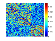
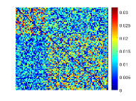
The first toy example is used to explain why we prefer multi-view learning rather than simply selecting a good view. We design a two-view synthetic dataset where each view is a 90 $\times$ 90 matrix with three 30 $\times$ 30 block matrices diagonally arranged. Without loss of generality, the data within each block denotes the affinity of two corresponding points in one cluster, while the data outside all of blocks denotes noise. Each element in all blocks is randomly generated in the range of 0 and 1, while the noise data is randomly generated in the range of 0 and e, where e is set as 0.6 in the 1st matrix, and 0.7 in the 2nd matrix. Following the complementary principle, in view 1 we increase the noise between the first and second block data to $e=0.8$, and increase the noise between the second and third block data to $e=1.0$. Then they are normalized to be that the sum of each row is 1. The original input graphs are shown in Figure 3. By performing CLR on each individual graph, their clustering performance are : ACC(Purity) of view 1 and 2 are 0.663/0.635, NMI of view 1 and 2 are 0.580/0.580. However, when CLR-IW is used to integrate these two complementary graphs, we recover the perfectly clean block diagonal matrix and the learned weights are 0.528/0.472, which indicates effectiveness of multi-view learning.

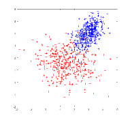
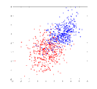
The second toy example works on a synthetic dataset given by [8] which contains two views that are showed as Fig. 4 (a) and (c) respectively. It can be observed that two-class samples are more discriminative in view 1 than they are in view 2. Thus, when each of them is applied to CLR, the similarity matrix $S$ learned by the former is more cleaner (See Fig. 4 (b) and (d). For better presentation, we normalize each similarity matrix by binaryzation in gray style). Table I shows the results of both single view clustering and iterative results using CLR-IW. It is seen that the ”$k=3$” obtains the best clustering result, whose ACC, NMI, and Purity reach up to 0.985, 0.889, and 0.985. Moreover, each single view learning results and ”$k=1$” being the baselines in this experiment, the generated CLR-IW has a noticeable improvement to them. Interestingly, since view 1 is stronger than view 2, the finally learned normalized weights are 0.538/0.462, which exactly agrees with our prior knowledge.

6.2 Datasets

The Datasets used in the following experiments are very popular in multi-view learning tasks, which are MSRC-v1 [49], Caltech101 [50], Handwritten numerals [51], NUS-WIDE Animals [52] and MNIST [53]. The brief description of each dataset is introduced as follows:

1) MSRC-v1: This collection is a scene recognition dataset which contains 240 images. Following [54], we select 7 classes which are composed of tree, building, airplane, cow, face, car, bicycle, and each class has 30 images. We extracted five visual features for each image: 24 Color Moment, 576 HOG, 512 GIST, 256 LBP, and 254 CENTRIST.

2) Caltech101: This dataset contains 8677 images which can be divided into 101 classes. We use two regular subsets Caltech101-7 and Caltech101-20 in our experiments. Six extracted features can be used, and they are 48 Gabor, 40 Wavelet Moments (WM), 254 CENTRIST, 1984 HOG, 512 GIST, 928 LBP.

3) Handwritten Numerals: This dataset is about handwritten numerals (0-9) extracted from a collection of Dutch utility maps. There are 2000 patterns and 200 for each class. These digits are represented as six public features: 76 Fourier coefficients of the character shapes (FOU), 216 profile correlations (FAC), 64 Karhunen-love coefficients (KAR), 240 pixel averages in 2 $\times$ 3 windows (PIX), 47 Zernike moment (ZER) and morphological (MOR) features.

4) NUS-WIDE: The dataset contains 269,648 images of 81 concepts. In our experiments, 12 categories about animal concept are selected and each contains 200 images. They are cat, cow, dog, elk, hawk, horse, lion, squirrel, tiger, whales, wolf, and zebra. Each image is represented by six type low-level features: 64 color histogram, 144 color correlogram, 73 edge direction histogram, 128 wavelet texture, 225 block-wise color moment and 500 bag of words based on SIFT descriptions.

5) MNIST: The dataset of handwritten digits (0-9) from Yann LeCun’s MNIST page has a test set of 10000 samples. There digits are described by three features: 30 isometric projection, 9 linear discriminant analysis and 30 neighborhood preserving embedding.

The statistics of these datasets are summarized in Table II, where MNIST is only for graph-free methods, since graph-based clustering method is time-consuming when datasize is very large. For the space limitation, we use the abbreviations (MSRC, Cal-7, Cal-20, HN, and NUS) for the name of each dataset.

TABLE II: Statistics of four datasets

Datasets	# of data	# of view	# of cluster
MSRC-v1	210	5	7
Caltech101	1474(2386)	6	7(20)
Handwritten Numerals	2000	6	10
NUS-WIDE	2400	6	12
MNIST	10000	3	10

6.3 Weight Learning Comparison

TABLE III: Summaries of formulations which are generated by employing different weight learning approaches for CLR learner, where the target variable $S$ is constrained as it is in Eq. (21), and $\alpha$ is constrained by $\mathcal{C}_{\alpha}$.

Methods	Objectives	Hyper-parameter (Grid search)	Referred work
CLR-NR	$\mathop{\min}\limits_{S,\alpha}\sum\limits_{v=1}^{M}{{\alpha_{v}}\left\|{S-{A^{(v)}}}\right\|_{F}^{2}}+{\gamma_{1}}\left\|\alpha\right\|_{2}^{2}$	${\gamma_{1}}\geq 0$, $[1,5,10,50,100,500,1000]$	[22, 23, 24, 25]
CLR-ER	$\mathop{\min}\limits_{S,\alpha}\sum\limits_{v=1}^{M}{\big{(}{{\alpha_{v}}\left\|{S-{A^{(v)}}}\right\|_{F}^{2}+{\gamma_{2}}{\alpha_{v}}\log{\alpha_{v}}}\big{)}}$	$\gamma_{2}\geq 0$, $[1,5,10,50,100,500,1000]$	[28, 29]
CLR-EF	$\mathop{\min}\limits_{S,\alpha}\sum\limits_{v=1}^{M}{\alpha_{v}^{{\gamma_{3}}}\left\|{S-{A^{\left(v\right)}}}\right\|_{F}^{2}}$	$\gamma_{3}\geq 1$, $[1.5,2.0,2.5,3.0,3.5,4.0]$	[30, 31, 23, 29, 32]
CLR-IW	$\mathop{\min}\limits_{S}\sum\limits_{v=1}^{M}{\left\|{S-{A^{\left(v\right)}}}\right\|_{F}^{p}}$	$0<p\leq 2$, $[0.1,0.4,0.7,1.0,1.3,1.7]$	-

(a) ACC

(b) NMI

(c) Purity

Figure 5: Clustering performance of the generated methods listed in Table III on various datasets.

(a) CLR-NR

(b) CLR-ER

(c) CLR-EF

(d) CLR-IW

Figure 6: Standard deviation of view weights for different methods on various datasets.

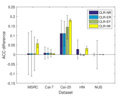
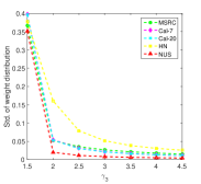
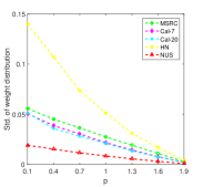
To quantitatively investigate the differences among all of aforementioned weight learning approaches, we do crosswise comparison by achieving each of them on CLR model rather than directly include any particular previous method. Their names, objectives, the corresponding parameters, and the referred work are showed in Table III. As a convention in [24, 23, 29, 31], grid search is adopted here to try the different values of the hyper-parameter for each compared method. Although it is known that the wider and denser the grid is, the better clustering performance will be, it is very hard to set the proper range and step size of them in practical applications. In this paper, we empirically set them as in third column of Table III after several small tests.

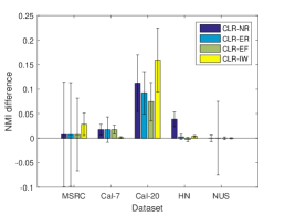
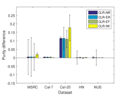
According to the analysis in Section 2, we easily come to the algorithm for each problem, which is ignorant in this part. It is obvious that each of them models a non-convex problem, since the rank constraint is always supposed to be satisfied. Considering that in most cases every view contributes to the final clustering results, we initialize each algorithm with the equal weights. Fig. 5 reports the clustering results on various datasets in terms of aforementioned three standard evaluation metrics respectively. Multi-view equal weights CLR is the potential baseline in this experiment, and the magnitude of a bar denotes how many improvements of each method makes. The standard deviation for each method is also presented by attaching the top of a bar.

At the first sight of Fig. 5, except NUS dataset, on which each method obtains the very close clustering results with equal weights version, it is observed that almost every method achieves better performance than the baseline, which indicates the weight learning does work for multi-clustering. More importantly, the best clustering results of CLR-IW most times are higher than others in compared schemes. It is because that the hyper-parameter for the intrinsic weight learning approach is searched in a interval with two-side boundary. On this event, grid search is often effective. Furthermore, from the standard deviation of each method, we know that the different values of hyper-parameter have an significant impact on the final clustering performance, and CLR-IW is robuster than any competing method.

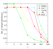
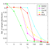
Another point which we concern is the learned view weights. Standard deviation (Std) is used to describe the smoothness of the learned weights as in Fig. 6. Generally, with the increase of the hyper-parameter in each compared method, Std is dropping sustainedly with a lower bound zero, which indicates the weights distributions are getting smoother. Particularly, when Std is zero, all of view weights become equal. In addition, we find that NR has the similar weight distributions with ER, which is apparently due the parallel type regularization form. As we analyze before, they both can learn the sparse weights, thus when the weight of regularization is small, it comes to very high Std. For EF, Std decreases dramatically when $\gamma_{3}$ varies form 1.5 to 2. As the adopted grid search is following [31], we do not subdivide this range any longer. Interestingly, when $\gamma_{3}>0$, EF is much similar with IW, i.e., they have the close values of Std and consistent order of datasets on each hyper-parameter point. The reason of this phenomenon can be simply explained as:

When Algorithm 1 converges, according to Eq. (12), we know that the normalized weight $\widetilde{\alpha_{v}}$ (like constraint $\mathcal{C}_{\alpha}$) can be represented as $\widetilde{{\alpha_{v}}}=\frac{{\frac{p}{2}\Phi_{v}^{\frac{{p-2}}{2}}}}{{\frac{p}{2}\sum\limits_{u=1}^{M}{\Phi_{u}^{\frac{{p-2}}{2}}}}}=\frac{1}{{\sum\limits_{u=1}^{M}{{{\left({\frac{{{\Phi_{v}}}}{{{\Phi_{u}}}}}\right)}^{\frac{2}{{p-2}}}}}}}$, which is identical with Eq. (8) when $p=2\gamma_{3}$.

Noting that the peak value in IW is not as large as other methods, which shows that IW actually prefers the smooth weight distribution.

6.4 Extension to Other Clustering Tasks

TABLE IV: Summaries of formulations which are generated by employing intrinsic weight learning approach for NMF and SC clustering model, where $0<p\leq 2$.

Methods	Objectives	Constriants
SC-IW	$\mathop{\min}\limits_{G}\sum\limits_{v=1}^{M}{{{\left({Tr\left({{G^{T}}LG}\right)}\right)}^{\frac{p}{2}}}}$	${G^{T}}G=I$, or ${G^{T}}DG=I$
NMF-IW	$\mathop{\min}\limits_{F^{(v)},G}\sum\limits_{v=1}^{M}{\left\|{{X^{{{(v)}}}}^{T}-G{F^{(v)}}^{T}}\right\|_{F}^{p}}$	${G_{ic}}\in\left\{{0,1}\right\},\sum\limits_{c=1}^{C}{{G_{ic}}}=1,\forall i=1,2,...,N$

Besides the recent clustering method CLR, the proposed intrinsic weight learning approach is easily extended to some other basic clustering approaches which produces more new multi-view clustering methods. Here we firstly introduce two base learners.

1. Spectral Clustering (SC) method is a representative paradigm for nonlinear data clustering. Given the adjacent matrix $W\in\mathbb{R}^{N\times N}$ (The corresponding degree matrix and Laplacian matrix is $D$ and $L$), the clustering objective is

   $$\mathop{\min}\limits_{G}Tr\left({{G^{T}}LG}\right).$$

   If the constraint to $G$ is $G^{T}G=I$, it will come to Ratio Cut (RC) problem, while if the constraint is $G^{T}DG=I$, it becomes Normalized Cut (NC) problem.

2. Previous work [55] proved that the G-orthogonal non-negative matrix factorization (NMF) is equivalent to relaxed $K$-means clustering, and the following objective which is formalized by NMF but embedding $K$-means is a popular clustering learner

   $$\begin{split}&\mathop{\min}\limits_{F,G}\left\|{{X^{T}}-G{F^{T}}}\right\|_{F}^{2}\\ s.t.\,{G_{ic}}\in&\left\{{0,1}\right\},\sum\limits_{c=1}^{C}{{G_{ic}}}=1,\forall i=1,2,...,N,\end{split}$$

   where $X\in\mathbb{R}^{d\times N}$ is the input data matrix with $N$ samples and $d$-dimensional feature, $F\in\mathbb{R}^{d\times C}$ is the cluster centroid matrix, and $G\in\mathbb{R}^{N\times C}$ is the cluster assignment matrix and whose each row is the 1-of-$C$ coding scheme.

By employing the proposed weight learning strategy to above two base learners, we obtain two multi-view clustering methods in Table IV. The optimization procedure for SC-IW is quite simple while it is not direct for NMF-IW. So we show the detailed steps for NMF-IW in Appendix. The clustering results on various datasets are presented in Tables V and VI, where we report the improvements of the best clustering performance relative to baselines. Since there are three metrics, we sum them up and find the largest one during the grid search.

Overall, we can see that with the use of intrinsic weight learning paradigm, the obtained clustering results apparently outperform baselines which does not take the discriminative view weights. Interestingly, it is observed that when intrinsic weight learning is applied in different base learners, the improvements sometimes discord. For instance, CLR-IW does not work well on NUS but SC-IW and NMF-IW do. This indicates that view weights are not absolute and actually much related to the specific model presentation capacity.

TABLE V: Improvements of SC-IW with multi-view equal weights SC being the baseline. (%)

		MSRC	Cal-7	Cal-20	HN	NUS
RC-IW	ACC	+0.48	+8.35	+8.22	+11.00	-1.30
	NMI	+1.40	+5.69	+3.82	+6.42	-1.37
	Purity	+4.29	-9.32	-3.18	+17.55	+14.17
NC-IW	ACC	+0.47	+6.31	-1.00	+2.35	-1.75
	NMI	+0.15	+1.77	+2.04	+2.61	-1.16
	Purity	+4.28	-6.55	+9.30	+9.85	+22.08

TABLE VI: Improvements of NMF-IW with multi-view equal weights NMF being the baseline. (%)

	MSRC	Cal-7	Cal-20	HN	NUS	MNIST
ACC	+9.00	+0.80	+3.23	+16.85	+6.00	+7.53
NMI	+4.90	+0.80	-0.58	+12.10	+3.48	+7.32
Purity	+8.60	+0.20	-1.34	+16.85	+6.34	+7.24

7 Conclusion

In this paper, we present a new weight learning strategy named Intrinsic Weight Learning Approach for multi-view clustering task. By comparing with several classical weight learning approaches both in theory and experiments, we conclude that the proposed intrinsic weight learning is robuster to hyper-parameter and easy to obtain the better results. Moreover, we show that the proposed weight learning approach can be naturally used in other basic clustering learners. Extensive experiments have shown that this weight learning approach significantly improves the clustering performance and practical to use. In the future work, like [56] we will consider formulating a general framework which can also work in semi-supervised context.

[The optimization procedure of solving NMF-IW problem] According to Algorithm 1, we know that the key step to address the NMF-IW problem is to solve the following subproblem

$$\mathop{\min}\limits_{\alpha,G,{F^{\left(v\right)}}}\sum\limits_{v=1}^{M}{{\alpha_{v}}\left\|{\mathop{{X^{\left(v\right)}}}\nolimits^{T}-G\mathop{{F^{\left(v\right)}}}\nolimits^{T}}\right\|}_{F}^{2},$$ (31)

where $\alpha$ is fixed. This problem can be solved by alternatively update $F^{(v)}$ and $G$ in each iteration. When $G$ is fixed, taking the derivative of Eq. (31) w.r.t $F^{(v)}$ and setting the derivatives to zeros, for each $1\leq v\leq M$, we have

$$\begin{split}&{\alpha_{v}}{\left({\mathop{{X^{\left(v\right)}}}\nolimits^{T}-G}\right)^{T}}\left({-G}\right)={\bf{0}}\\ \Rightarrow&{F^{\left(v\right)}}=XG{\left({{G^{T}}G}\right)^{-1}}.\end{split}$$ (32)

When $G$ is fixed, Eq. (31) can be split into $n$ smaller subproblems, each of which can be written as ($1\leq i\leq N$)

$$\mathop{\min}\limits_{{g_{i}}}\sum\limits_{v=1}^{M}{\left\|{{x^{i}}-{g_{i}}\mathop{{F^{\left(v\right)}}}\nolimits^{T}}\right\|_{2}^{2}}\quad{g_{i}}\in\left\{{0,1}\right\},\sum\limits_{c=1}^{C}{{g_{ic}}}=1.$$ (33)

Seeing that $g_{i}$ satisfied $1$-$of$-$C$ coding scheme, there are $C$ candidates to be the solution of Eq. (33), each of which is the $c$-th row of matrix ${I_{C}}=\left[{{{\bf{e}}_{1}};{{\bf{e}}_{2}};...;{{\bf{e}}_{C}}}\right]$. This problem can be effectively solved by exhaustively searching strategy if $C$ is not very large.

References

- [1] B. Schölkopf, A. J. Smola, and K. Müller, “Nonlinear component analysis as a kernel eigenvalue problem,” Neural Computation, vol. 10, no. 5, pp. 1299–1319, 1998.
- [2] J. Shi and J. Malik, “Normalized cuts and image segmentation,” IEEE Trans. Pattern Anal. Mach. Intell., vol. 22, no. 8, pp. 888–905, 2000.
- [3] B. J. Frey and D. Dueck, “Clustering by passing messages between data points,” science, vol. 315, no. 5814, pp. 972–976, 2007.
- [4] C. Xu, D. Tao, and C. Xu, “A survey on multi-view learning,” CoRR, vol. abs/1304.5634, 2013.
- [5] C.-D. Wang, J.-H. Lai, and S. Y. Philip, “Multi-view clustering based on belief propagation,” IEEE Transactions on Knowledge and Data Engineering, vol. 28, no. 4, pp. 1007–1021, 2016.
- [6] S. Bickel and T. Scheffer, “Multi-view clustering.” in ICDM, vol. 4, 2004, pp. 19–26.
- [7] P. Muthukrishnan, D. Radev, and Q. Mei, “Edge weight regularization over multiple graphs for similarity learning,” in Data Mining (ICDM), 2010 IEEE 10th International Conference on. IEEE, 2010, pp. 374–383.
- [8] A. Kumar, P. Rai, and H. Daume, “Co-regularized multi-view spectral clustering,” in Advances in neural information processing systems, 2011, pp. 1413–1421.
- [9] A. Kumar and H. Daumé, “A co-training approach for multi-view spectral clustering,” in Proceedings of the 28th International Conference on Machine Learning (ICML-11), 2011, pp. 393–400.
- [10] W. Tang, Z. Lu, and I. S. Dhillon, “Clustering with multiple graphs,” in Data Mining, 2009. ICDM’09. Ninth IEEE International Conference on. IEEE, 2009, pp. 1016–1021.
- [11] T. Xia, D. Tao, T. Mei, and Y. Zhang, “Multiview spectral embedding,” IEEE Transactions on Systems, Man, and Cybernetics, Part B (Cybernetics), vol. 40, no. 6, pp. 1438–1446, 2010.
- [12] J. Liu, C. Wang, J. Gao, and J. Han, “Multi-view clustering via joint nonnegative matrix factorization,” in Proceedings of the 2013 SIAM International Conference on Data Mining. SIAM, 2013, pp. 252–260.
- [13] X. Cai, F. Nie, H. Huang, and F. Kamangar, “Heterogeneous image feature integration via multi-modal spectral clustering,” in Computer Vision and Pattern Recognition (CVPR), 2011 IEEE Conference on. IEEE, 2011, pp. 1977–1984.
- [14] H.-C. Huang, Y.-Y. Chuang, and C.-S. Chen, “Affinity aggregation for spectral clustering,” in Computer Vision and Pattern Recognition (CVPR), 2012 IEEE Conference on. IEEE, 2012, pp. 773–780.
- [15] Y. Li, F. Nie, H. Huang, and J. Huang, “Large-scale multi-view spectral clustering via bipartite graph.” in AAAI, 2015, pp. 2750–2756.
- [16] M. B. Blaschko and C. H. Lampert, “Correlational spectral clustering,” in Computer Vision and Pattern Recognition, 2008. CVPR 2008. IEEE Conference on. IEEE, 2008, pp. 1–8.
- [17] K. Chaudhuri, S. M. Kakade, K. Livescu, and K. Sridharan, “Multi-view clustering via canonical correlation analysis,” in Proceedings of the 26th annual international conference on machine learning. ACM, 2009, pp. 129–136.
- [18] N. Dalal and B. Triggs, “Histograms of oriented gradients for human detection,” in Computer Vision and Pattern Recognition, 2005. CVPR 2005. IEEE Computer Society Conference on, vol. 1. IEEE, 2005, pp. 886–893.
- [19] R. Xia, Y. Pan, L. Du, and J. Yin, “Robust multi-view spectral clustering via low-rank and sparse decomposition.” in AAAI, 2014, pp. 2149–2155.
- [20] Y. Wang, W. Zhang, L. Wu, X. Lin, M. Fang, and S. Pan, “Iterative views agreement: An iterative low-rank based structured optimization method to multi-view spectral clustering,” in Proceedings of the Twenty-Fifth International Joint Conference on Artificial Intelligence, IJCAI 2016, New York, NY, USA, 9-15 July 2016, 2016, pp. 2153–2159.
- [21] Y. Cheng and R. Zhao, “Multiview spectral clustering via ensemble,” in Granular Computing, 2009, GRC’09. IEEE International Conference on. IEEE, 2009, pp. 101–106.
- [22] H. Cai, P. Ruan, M. Ng, and T. Akutsu, “Feature weight estimation for gene selection: a local hyperlinear learning approach,” BMC bioinformatics, vol. 15, no. 1, p. 70, 2014.
- [23] Y.-M. Xu, C.-D. Wang, and J.-H. Lai, “Weighted multi-view clustering with feature selection,” Pattern Recognition, vol. 53, pp. 25–35, 2016.
- [24] A. Kumar and B. Raj, “Unsupervised fusion weight learning in multiple classifier systems,” arXiv preprint arXiv:1502.01823, 2015.
- [25] M. Karasuyama and H. Mamitsuka, “Multiple graph label propagation by sparse integration,” IEEE transactions on neural networks and learning systems, vol. 24, no. 12, pp. 1999–2012, 2013.
- [26] J. Duchi, S. Shalev-Shwartz, Y. Singer, and T. Chandra, “Efficient projections onto the -ball for learning in high dimensions,” in Proceedings of the 25th international conference on Machine learning. ACM, 2008, pp. 272–279.
- [27] E. T. Jaynes, “Information theory and statistical mechanics,” Physical review, vol. 106, no. 4, p. 620, 1957.
- [28] T. Lange and J. M. Buhmann, “Fusion of similarity data in clustering,” in NIPS, 2005, pp. 723–730.
- [29] G.-Y. Zhang, D. Huang, C.-D. Wang, and W.-S. Zheng, “Weighted multi-view on-line competitive clustering,” in Big Data Computing Service and Applications (BigDataService), 2016 IEEE Second International Conference on. IEEE, 2016, pp. 286–292.
- [30] Z. Xue, G. Li, S. Wang, C. Zhang, W. Zhang, and Q. Huang, “Gomes: A group-aware multi-view fusion approach towards real-world image clustering,” in Multimedia and Expo (ICME), 2015 IEEE International Conference on. IEEE, 2015, pp. 1–6.
- [31] G. Tzortzis and A. Likas, “Kernel-based weighted multi-view clustering,” in Data Mining (ICDM), 2012 IEEE 12th International Conference on. IEEE, 2012, pp. 675–684.
- [32] G. F. Tzortzis and A. C. Likas, “Multiple view clustering using a weighted combination of exemplar-based mixture models,” IEEE Transactions on neural networks, vol. 21, no. 12, pp. 1925–1938, 2010.
- [33] C. L. Lawson, Contributions to the theory of linear least maximum approximation. University of California, 1961.
- [34] A. E. Beaton and J. W. Tukey, “The fitting of power series, meaning polynomials, illustrated on band-spectroscopic data,” Technometrics, vol. 16, no. 2, pp. 147–185, 1974.
- [35] F. Nie, J. Yuan, and H. Huang, “Optimal mean robust principal component analysis,” in Proceedings of the 31st international conference on machine learning (ICML-14), 2014, pp. 1062–1070.
- [36] R. Chartrand and W. Yin, “Iteratively reweighted algorithms for compressive sensing,” in Acoustics, speech and signal processing, 2008. ICASSP 2008. IEEE international conference on. IEEE, 2008, pp. 3869–3872.
- [37] I. Daubechies, R. DeVore, M. Fornasier, and C. S. Güntürk, “Iteratively reweighted least squares minimization for sparse recovery,” Communications on Pure and Applied Mathematics, vol. 63, no. 1, pp. 1–38, 2010.
- [38] F. Nie, H. Huang, X. Cai, and C. H. Ding, “Efficient and robust feature selection via joint -norms minimization,” in Advances in neural information processing systems, 2010, pp. 1813–1821.
- [39] L. Zelnik-Manor and P. Perona, “Self-tuning spectral clustering,” 2005.
- [40] D. Cai, X. He, and J. Han, “Document clustering using locality preserving indexing,” Knowledge and Data Engineering, IEEE Transactions on, vol. 17, no. 12, pp. 1624–1637, 2005.
- [41] F. Nie, X. Wang, and H. Huang, “Clustering and projected clustering with adaptive neighbors,” in The 20th ACM SIGKDD International Conference on Knowledge Discovery and Data Mining, KDD ’14, New York, NY, USA - August 24 - 27, 2014, 2014, pp. 977–986.
- [42] J. Feng, Z. Lin, H. Xu, and S. Yan, “Robust subspace segmentation with block-diagonal prior,” in Proceedings of the IEEE Conference on Computer Vision and Pattern Recognition, 2014, pp. 3818–3825.
- [43] J. Chen and J. Dy, “A generative block-diagonal model for clustering,” in Proceedings of the Thirty-Second Conference on Uncertainty in Artificial Intelligence, UAI 2016, June 25-29, 2016, New York City, NY, USA, 2016.
- [44] F. Nie, X. Wang, M. I. Jordan, and H. Huang, “The constrained laplacian rank algorithm for graph-based clustering.” in AAAI. Citeseer, 2016, pp. 1969–1976.
- [45] B. Mohar, Y. Alavi, G. Chartrand, and O. Oellermann, “The laplacian spectrum of graphs,” Graph theory, combinatorics, and applications, vol. 2, no. 871-898, p. 12, 1991.
- [46] F. R. Chung, Spectral graph theory. American Mathematical Soc., 1997, vol. 92.
- [47] K. Fan, “On a theorem of weyl concerning eigenvalues of linear transformations ii,” Proceedings of the National Academy of Sciences, vol. 36, no. 1, pp. 31–35, 1950.
- [48] R. Varshavsky, M. Linial, and D. Horn, “Compact: A comparative package for clustering assessment,” in Parallel and Distributed Processing and Applications-ISPA 2005 Workshops. Springer, 2005, pp. 159–167.
- [49] J. M. Winn and N. Jojic, “LOCUS: learning object classes with unsupervised segmentation,” in 10th IEEE International Conference on Computer Vision (ICCV 2005), 17-20 October 2005, Beijing, China, 2005, pp. 756–763.
- [50] L. Fei-Fei, R. Fergus, and P. Perona, “Learning generative visual models from few training examples: An incremental bayesian approach tested on 101 object categories,” Computer Vision and Image Understanding, vol. 106, no. 1, pp. 59–70, 2007.
- [51] A. Asuncion and D. Newman, “Uci machine learning repository,” 2007.
- [52] T.-S. Chua, J. Tang, R. Hong, H. Li, Z. Luo, and Y. Zheng, “Nus-wide: a real-world web image database from national university of singapore,” in Proceedings of the ACM international conference on image and video retrieval. ACM, 2009, p. 48.
- [53] Y. LeCun, C. Cortes, and C. J. Burges, “Mnist handwritten digit database,” AT&T Labs [Online]. Available: http://yann. lecun. com/exdb/mnist, vol. 2, 2010.
- [54] K. Grauman and T. Darrell, “Unsupervised learning of categories from sets of partially matching image features,” in Computer Vision and Pattern Recognition, 2006 IEEE Computer Society Conference on, vol. 1. IEEE, 2006, pp. 19–25.
- [55] C. Ding, X. He, and H. Simon, “Nonnegative lagrangian relaxation of k-means and spectral clustering,” Machine Learning: ECML 2005, pp. 530–538, 2005.
- [56] F. Nie, J. Li, X. Li et al., “Parameter-free auto-weighted multiple graph learning: A framework for multiview clustering and semi-supervised classification.” in IJCAI, 2016, pp. 1881–1887.