Sparse Spectrum Gaussian Process for Bayesian Optimization

Abstract

We propose a novel sparse spectrum approximation of Gaussian process (GP) tailored for Bayesian optimization. Whilst the current sparse spectrum methods provide desired approximations for regression problems, it is observed that this particular form of sparse approximations generates an overconfident GP, i.e. it produces less epistemic uncertainty than the original GP. Since the balance between predictive mean and the predictive variance is the key determinant to the success of Bayesian optimization, the current sparse spectrum methods are less suitable for it. We derive a new regularized marginal likelihood for finding the optimal frequencies to fix this over-confidence issue, particularly for Bayesian optimization. The regularizer trades off the accuracy in the model fitting with targeted increase in the predictive variance of the resultant GP. Specifically, we use the entropy of the global maximum distribution from the posterior GP as the regularizer that needs to be maximized. Since this distribution cannot be calculated analytically, we first propose a Thompson sampling based approach and then a more efficient sequential Monte Carlo based approach to estimate it. Later, we also show that the Expected Improvement acquisition function can be used as a proxy for the maximum distribution, thus making the whole process further efficient. Experiments show considerable improvement to Bayesian optimization convergence rate over the vanilla sparse spectrum method and over a full GP when its covariance matrix is ill-conditioned due to the presence of large number of observations.

1 Introduction

Bayesian optimization (BO) is a leading method for global optimization for expensive black-box functions [1, 2, 3, 4]. It is widely used in hyperparameter tuning of massive neural networks [5, 6], some of which can take days to train. It has also been used for optimization of physical products and processes [7] where one experiment can cost days, and experiments can also be expensive in terms of material cost. However, there could be scenarios when a large number of observations is available from priors or during the experiments. For example, in transfer learning, where many algorithms [8, 9, 10] pool existing observations from source tasks together for use in the optimization of a target task. Then even though the target function is expensive, the number of observations can be large if the number of source tasks is large and/or the number of observations from each source is large. Another scenario where we may have a large number of observations is when we deal with optimization of objective functions which are not very costly. For example, consider the cases when Bayesian optimization is performed using simulation software. They are often used in the early stage of a product design process to reduce a massive search space to a manageable one before real products are made. Whilst evaluation, a few thousands may be feasible, but millions are not because each evaluation can still take from several minutes to hours. We term this problem as a semi-expensive optimization problem. Such problems cannot be handled by the traditional global optimizers which often require more than thousands of evaluations. Bayesian optimization will also struggle, because its main ingredient, Gaussian process (GP) does not scale well beyond few hundreds of observations. In this paper, we address the scalability issue of GP for Bayesian optimization for such scenarios where a large number of observations appear naturally.

The scalability issue for Bayesian optimization has been previously addressed in two main ways: 1) by replacing GP with a more scalable Bayesian model, e.g. using Bayesian neural network [11] or random forest [12], or 2) by making sparse approximation of the full GP. The latter is often desirable as it still maintains the principled Bayesian formalism of GP. There are many sparse models in the literature, such as fully independent training conditional (FITC) [13, 14] which induces pseudo inputs to approximate the full GP, and variational approximation [15] which learns inducing inputs and hyperparameters by minimizing the KL divergence between the true posterior GP and an approximate one. Another line of work involves approximating a stationary kernel function using a sparse set of frequencies in its spectrum domain representation, e.g. sparse spectrum Gaussian process (SSGP) [16]. These methods suffer from either variance under-estimation (i.e., over-confidence) [13, 16] or over-estimation [15] and thus may hamper BO as the balance between predictive mean and variance is important to the success of BO. Recently, [17] has proposed variational Fourier features (VFF), which combines variational approximation and spectral representation of GP together and plausibly can approximate both mean and variance well. However, it is difficult to extend VFF to multiple dimensional problems, since a) the number of inducing variables grows exponentially with dimensions if the Kronecker kernel is used, or b) the correlation between dimensions would be ignored if an additive kernel is used.

In this paper, we aim to develop a sparse GP model tailored for Bayesian optimization. We propose a novel modification to the sparse spectrum Gaussian process approach to make it more suitable for Bayesian optimization. The main intuition that drives our solution is that while being over-confident at some regions is not very critical to Bayesian optimization when those regions have both low predictive value and low predictive variance. However, being over-confident in the regions where either predictive mean or predictive variance is high would be quite detrimental to Bayesian optimization. Hence, a targeted fixing may be enough to make the sparse models suitable for BO. An overall measure of goodness of GP approximation for BO would be to look at the global maximum distribution (GMD) [18, 19] from the posterior GP and check its difference to that of the full GP. Fixing over-confidence in the important regions may be enough to make the GMD of the sparse GP closer to that of the full GP. The base method in our work (SSGP) is known to under-estimate variance, which is why we need maximizing the entropy of GMD. Following this idea, we add entropy of the maximum distribution as a new regularization term that is to be maximized in conjunction with the marginal likelihood so that the optimal sparse set of the frequencies are not only benefit for model fitting, but also fixes the over-confidence issue from the perspectives of the Bayesian optimization.

We first provide a Thompson sampling approach to estimate the maximum distribution for the sparse GP, and then propose a more efficient sequential Monte Carlo based approach. This approach provides efficiency as many Monte Carlo samples can be reused during the optimization for the optimal frequencies. Moreover, the maximum distribution also does not change much between two consecutive iterations of Bayesian optimization as the GP differs by only one observation. Later, we empirically show that Expected Improvement acquisition function can be used as a proxy of the maximum distribution, significantly improving the computational efficiency. We demonstrate our method on two synthetic functions and two real world problems, one involving hyperparameter optimization in a transfer learning setting and another involving alloy design using a thermodynamic simulator. In all the experiments our method provides superior convergence rate over standard sparse spectrum methods. Additionally, our method also performs better than the full GP when the covariance matrix faces ill-conditioning due to large number of observations placed close to each other.

2 Background

We consider the maximization problem $\boldsymbol{x}^{*}=\text{argmax}_{\boldsymbol{x}\in\mathcal{X}}f(\boldsymbol{x})$, where $f:\boldsymbol{x}\rightarrow\mathbb{R}$, $\mathcal{X}$ is a compact subspace in $\mathbb{R}^{d}$, and $\boldsymbol{x}^{*}$ is the global maximizer.

2.1 Bayesian optimization

Bayesian optimization includes two main components. It first uses a probabilistic model, typically a GP, to model the latent function and then constructs a surrogate utility function, or acquisition function which encapsulates optimistic estimate of the goodness about the next query.

Gaussian process [20] provides a distribution over the space of functions and it can be specified by a mean function $\mu(\boldsymbol{x})$ and a covariance function $k(\boldsymbol{x},\boldsymbol{x}^{\prime})$. A sample from a GP is a function $f(\boldsymbol{x})\sim\mathcal{GP}(\mu(\boldsymbol{x}),k(\boldsymbol{x},\boldsymbol{x}^{\prime}))$. Without loss of generality, we often assume that the prior mean function is zero function and thus GP can be fully defined by $k(\boldsymbol{x},\boldsymbol{x}^{\prime})$. The squared exponential kernel and the Mat$\acute{e}$rn kernel are popular choices of $k$.

In GP, the joint distribution for any finite set of random variables are multivariate Gaussian distribution. Given a set of noisy observations $\mathcal{D}_{t}=\{\boldsymbol{x}_{i},y_{i}\}_{i=1}^{t}$, where $y_{i}=f_{i}+\varepsilon_{i}$ with $\varepsilon_{i}\sim\mathcal{N}(0,\sigma_{n}^{2})$, the predictive distribution of $y_{t+1}$ in GP follows a normal distribution $p(f_{t+1}|\mathcal{D}_{t},\boldsymbol{x}_{t+1})=\mathcal{N}(\mu(\boldsymbol{x}_{t+1}),\sigma^{2}(\boldsymbol{x}_{t+1}))$ with

$$\mu(\boldsymbol{x}_{t+1}) =\mathbf{k}^{T}\left[\mathbf{K}+\sigma_{n}^{2}\mathbf{I}\right]^{-1}\boldsymbol{Y}$$ (1)

$$\sigma^{2}(\boldsymbol{x}_{t+1}) =k(\boldsymbol{x}_{t+1},\boldsymbol{x}_{t+1})-\mathbf{k}^{T}\left[\mathbf{K}+\sigma_{n}^{2}\mathbf{I}\right]^{-1}\mathbf{k}\text{,}$$ (2)

where $\mathbf{k}=\left[k(\boldsymbol{x}_{t+1},\boldsymbol{x}_{1}),k(\boldsymbol{x}_{t+1},\boldsymbol{x}_{2}),\cdots,k(\boldsymbol{x}_{t+1},\boldsymbol{x}_{t})\right]$, $\boldsymbol{Y}=\{y_{i}\}_{i=1}^{t}$and $\mathbf{K}$ is the Gram matrix.

The posterior computation of GP involves the inversion of the Gram matrix and it would be very costly for a large number of observations. Sparse approximation is the usual way to reduce the computational cost with slight reduction in modeling accuracy. In this paper we focus on the SSGP for optimization purpose due to its simplification and scalability, details of which is discussed in the following subsection.

Once the GP has been built to model the latent function, we can construct acquisition functions by combining the predictive mean and variance of the posterior GP to find the next query. Some popular acquisition functions include expected improvement (EI), and GP-UCB [21, 29] . We use EI function since it can work well. The EI is defined as the expected improvement over the current maximal value $f(\boldsymbol{x}^{+})$. The analytic form of EI can be derived as [1]

$$\alpha_{EI}(\boldsymbol{x})=\begin{cases}\sigma(\boldsymbol{x})Z\Phi(Z)+\sigma(\boldsymbol{x})\phi(Z)&\sigma(\boldsymbol{x})>0\\ 0&\sigma(\boldsymbol{x})=0\end{cases},$$

where $Z=\left[\mu(\boldsymbol{x})-f(\boldsymbol{x}^{+})\right]/\sigma(\boldsymbol{x}).$ $\Phi(Z)$ and $\phi(Z)$ are the cumulative distribution function and probability density function of the standard normal distribution, respectively.

2.2 Sparse spectrum Gaussian process

Sparse Gaussian process often introduce inducing points to approximate the posterior mean and variance of full GP whilst sparse spectrum Gaussian process uses optimal spectrum frequencies to approximate the kernel function. Briefly, according to the Bochner’s theorem [22], any stationary covariance function can be represented as the Fourier transform of some finite measure $\sigma_{f}^{2}p(\mathbf{s})$ with $p(\mathbf{s})$ a probability density as

$$k(\boldsymbol{x}_{i},\boldsymbol{x}_{j})=\int_{\mathbb{R}^{D}}e^{2\pi i\mathbf{\boldsymbol{s}}^{T}(\boldsymbol{x}_{i}-\boldsymbol{x}_{j})}\sigma_{f}^{2}p(\mathbf{s})d\mathbf{s},$$ (3)

where the frequency vector $\mathbf{s}$ has the same length $D$ as the input vector $\boldsymbol{x}$. In other words, a spectral density entirely determines the properties of a stationary kernel. Furthermore, Eq.(3) can be computed and approximated as

$$k(\boldsymbol{x}_{i},\boldsymbol{x}_{j}) =\sigma_{f}^{2}\mathbb{E}_{p(\mathbf{s})}\left[e^{2\pi i\mathbf{s}^{T}\boldsymbol{x}_{i}}(e^{2\pi i\mathbf{s}^{T}\boldsymbol{x}_{j}})^{*}\right]$$

$$\simeq\frac{\sigma_{f}^{2}}{m}\stackrel{{\scriptstyle[}}{{r}}=1]{m}{\mathbf{\boldsymbol{\sum}}}\mathrm{cos}\left[2\pi\boldsymbol{s}_{r}^{T}(\boldsymbol{x}_{i}-\boldsymbol{x}_{j})\right]$$ (4)

$$=\frac{\sigma_{f}^{2}}{m}\phi(\boldsymbol{x}_{i})^{T}\phi(\boldsymbol{x}_{j}).$$ (5)

The Eq.(4) is obtained by Monte Carlo approximation with symmetric sets $\{\mathbf{s}_{r},-\mathbf{s}_{r}\}_{r=1}^{m}$ sampled from $\mathbf{s}_{r}\sim p(\mathbf{s})$, where $m$ is the number of spectral frequencies (features). To obtain the Eq.(5), we use the setting

$$\phi(\boldsymbol{x})=[\mathrm{cos}(2\pi\boldsymbol{s}_{1}^{T}\boldsymbol{x}),\,\mathrm{sin}(2\pi\boldsymbol{s}_{1}^{T}\boldsymbol{x}),\cdots,\\ \,\mathrm{cos}(2\pi\boldsymbol{s}_{m}^{T}\boldsymbol{x}),\,\mathrm{sin}(2\pi\boldsymbol{s}_{m}^{T}\boldsymbol{x})]^{T},$$ (6)

which is a column vector of length 2$m$ containing the evaluation of the $m$ pairs of trigonometric functions at $\boldsymbol{x}$. Then, it is straightforward to compute the posterior mean and variance of SSGP

$$\mu(\boldsymbol{x}_{t+1}) =\phi(\boldsymbol{x}_{t+1})^{T}\mathbf{A}^{-1}\boldsymbol{\Phi}\boldsymbol{Y}$$ (7)

$$\sigma^{2}(\boldsymbol{x}_{t+1}) =\sigma_{n}^{2}+\sigma_{n}^{2}\phi(\boldsymbol{x}_{t+1})^{T}\mathbf{A}^{-1}\phi(\boldsymbol{x}_{t+1}),$$ (8)

where $\boldsymbol{\Phi}=[\phi(\boldsymbol{x}_{1}),\ldots\,,\phi(\boldsymbol{x}_{t})]\in\mathbb{R}^{2m\times t}$ and $\mathbf{A}=\boldsymbol{\Phi}\boldsymbol{\Phi}^{T}+\frac{m\sigma_{n}^{2}}{\sigma_{f}^{2}}\mathbf{I}_{2m}$. To select optimal frequencies, we can maximize the log marginal likelihood $\mathrm{log}p(\boldsymbol{Y}|\varTheta)$, where $\varTheta$ is the set of all hyperparameters in the kernel function and the spectrum frequencies,

$$\mathrm{log}p(\boldsymbol{Y}|\varTheta) =-\frac{1}{2\sigma_{n}^{2}}[\boldsymbol{Y}^{T}\boldsymbol{Y}-\boldsymbol{Y}^{T}\boldsymbol{\Phi}^{T}\mathbf{A}^{-1}\boldsymbol{\Phi}\boldsymbol{Y}]$$

$$-\frac{1}{2}\mathrm{log}|\mathbf{A}|+m\mathrm{log}\frac{m\sigma_{n}^{2}}{\sigma_{f}^{2}}-\frac{t}{2}\mathrm{log}2\pi\sigma_{n}^{2}.$$ (9)

The SSGP, therefore, uses $m$ optimal frequencies to approximate the full GP, which reduces the computational complexity to $\mathcal{O}(tm^{2})$, and provides computational efficiency if $m\ll t$.

(a) full GP

(b) SSGP

(c) RSSGP

(d) RSSGP using EI as a proxy

Figure 1: (a)-(c) The visualization of overconfidence of SSGP on the GMD. The upper graphs show 200 posterior samples of Sinc function, modeled by (a) full GP, (b) SSGP with 30 optimal frequencies, and (c) RSSGP with 30 optimal frequencies. The red circle denotes observation and the blue circle denotes the maximum location of a posterior sample. The lower graphs illustrate the resultant GMD respectively. The $\mathrm{\mathbb{H}}\left[\mathrm{GMD}\right]$ is the entropy of the GMD. We can see the GMD of RSSGP is closer to that of full GP than SSGP. (d) RSSGP with 30 optimal frequencies by using the EI function as a proxy to the regularization. Its GMD is at the middle and the EI function is at the bottom.

3 Bayesian optimization using regularized sparse spectrum Gaussian process

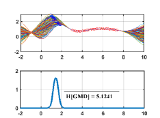
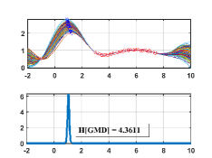
The naive SSGP can be directly used for Bayesian optimization by replacing the full GP. However, the SSGP was designed for a regression task, which means that it assigns modeling resources equally over the whole support space. Moreover, it leads to overconfidence on the GMD of interest in BO. We illustrate the overconfidence of the SSGP in Figure 1a-1b, where the GMD of SSGP in 1b (bottom) is narrower and sharper than that in the 1a, which is the GMD of the full GP.

To overcome this overconfidence, we propose a novel and scalable sparse spectrum Gaussian procesprobability of improvement,s model tailoring for BO. Our approach involves maximizing a new loss function to select the optimal spectrum frequencies. We design the loss function to include the marginal likelihood in the SSGP and a regularization term, which has the goal of minimizing the difference between the GMD of the full GP and that of the proposed sparse approximation. We denote our proposed sparse spectrum model as the regularized SSGP (RSSGP). For the sake of convenience, we denote the GMD of the full GP as $p(\boldsymbol{x}^{*})$ and that of RSSGP as $q(\boldsymbol{x}^{*})$.

We first discuss the choice for the regularization term. Whilst the KL divergence $D_{KL}(q\,||\,p)$ seems to be the solution to measure difference between two distributions, it is not feasible in our scenario as we cannot access $p(\boldsymbol{x}^{*})$. Nevertheless, the property that the SSGP tends to be over-fitting implies that the entropy for the GMD in SSGP would be smaller than that of the full GP.Therefore, we can use the entropy of $q(\boldsymbol{x}^{*})$, or $\mathrm{\mathbb{H}}[q(\boldsymbol{x}^{*})]$ as the regularization term in the loss function that needs to be maximized. In this way, the resultant sparse GP would minimize the difference between $q(\boldsymbol{x}^{*})$ and $p(\boldsymbol{x}^{*})$. Formally, the loss function in RSSGP is defined as

$$\mathcal{L}=\mathrm{log}p(\boldsymbol{Y}|\varTheta)+\lambda\mathrm{log}\mathrm{\mathbb{H}}\left[q(\boldsymbol{x}^{*})\right],$$ (10)

where the first term is the log marginal likelihood as Eq.(9) in SSGP, the second term is the entropy for the posterior distribution of the global maximizer $q(\boldsymbol{x}^{*})$ and $\lambda$ is the trade-off parameter. Now we can obtain $\varTheta$ by maximizing the loss function

$$\varTheta=\mathrm{argmax}\mathrm{log}p(\boldsymbol{Y}|\varTheta)+\lambda\mathrm{log}\mathrm{\mathbb{H}}\left[q(\boldsymbol{x}^{*})\right].$$ (11)

The questions break down to that how $q(\boldsymbol{x}^{*})$ can be computed and how $q(\boldsymbol{x}^{*})$ is relevant to the spectrum frequencies. Next, knowing there is no analytical form for $q(\boldsymbol{x}^{*})$, we propose two methods to estimate $q(\boldsymbol{x}^{*})$. One is Thompson sampling and the other is a sequential Monte Carlo approach that takes less computation. We also propose a significantly computationally-efficient approximation by treating the EI acquisition function as a proxy of $q(\boldsymbol{x}^{*})$.

3.1 Thompson sampling based approach

In this section we demonstrate how to approximate $q(\boldsymbol{x}^{*})$ by following the work of [19]. In Thompson sampling (TS), one uses a linear model to approximate the function $f(\boldsymbol{x})=\phi(\boldsymbol{x})^{T}\bar{\boldsymbol{\theta}}$ where $\bar{\boldsymbol{\theta}}\backsim\mathcal{N}(\boldsymbol{0},\mathbf{I})$ is a standard Gaussian. Giving observed data $\mathcal{D}_{t}$, the posterior of $\bar{\boldsymbol{\theta}}$ conditioning $\mathcal{D}_{t}$ is a normal $\mathcal{N}(\mathbf{A}^{-1}\boldsymbol{\Phi}^{T}\boldsymbol{Y},\mathbf{A}^{-1}\sigma_{n}^{2})$, where $\mathbf{A}$ and $\boldsymbol{\Phi}$ have already been defined in Eq.(7). Note that $\phi(\boldsymbol{x})$ is a set of random Fourier features in the traditional TS while $\phi(\boldsymbol{x})$ is a set of $m$ pairs of symmetric Fourier features in our framework.

To estimate the global maximum distribution in RSSGP, we let $\phi_{i}$ and $\bar{\boldsymbol{\theta}}_{i}$ be a random set of $m$ pairs of features and corresponding posterior weights. Both are sampled according to the generative process above and they can be used to construct a sampled function $f_{i}(\boldsymbol{x})=\phi_{i}(\boldsymbol{x})^{T}\bar{\boldsymbol{\theta}_{i}}$. We can maximize this function to obtain a sample $\boldsymbol{x}_{i}^{*}$. Once we have acquired sufficient samples, we use histogram based method to obtain the probability mass function (PMF) over all $\boldsymbol{x}^{*}$, denoted as $F(\boldsymbol{x}^{*})$. Then we estimate the entropy via $\mathrm{\mathbb{H}}\left[q(\boldsymbol{x}^{*})\right]=-\sum_{i=1}^{L}F(\boldsymbol{x}_{i}^{*})\,\mathrm{log}F(\boldsymbol{x}_{i}^{*})$, where $L$ is the number of samples. Since our RSSGP uses Fourier features $\phi(\boldsymbol{x})$ to approximate a stationary kernel function, and $q(\boldsymbol{x}^{*})$ also changes with applying different Fourier features, therefore we can obtain the optimal features by maximizing the combined term $\mathcal{L}$ in Eq.(10). As a result, the selected optimal frequencies in RSSGP are not only take care of posterior mean approximation, but also maximize the entropy of $q(\boldsymbol{x}^{*})$. This is the key reason why we choose SSGP as our base sparse method. Sparse models like FITC and VFE are not capable with this idea since we cannot relate their sparse sets to their GMDs due to the insufficient researches in this area.

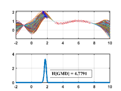
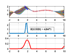
We illustrate the GMD of RSSGP in Figure 1c. We can see that it is closer to the GMD of the full GP than that of SSGP. All the GMDs in Figure 1 are estimated via TS.

(a) MC performance

(b) TS performance

Figure 2: MC approach vs TS approach. The blue lines show the reference $p(\boldsymbol{x}^{*})$ distribution, while the red lines illustrate the approximation using MC (a) and TS (b) given the same running time.

3.2 Monte Carlo based approach

The estimation of $q(\boldsymbol{x}^{*})$ by TS often requires thousands of samples (e.g, $L$), one of which involves the inversion of a $m\times m$ matrix. Inspired by a recent work [23] employing sequential Monte Carlo algorithm to approximate the GMD, we develop an intensive approach to estimate $q(\boldsymbol{x}^{*})$ in RSSGP with significantly less computation.

We start with $n_{p}$ particles at positions $\boldsymbol{\bar{x}}^{1},\ldots,\boldsymbol{\bar{x}}^{n_{p}}$. Then we assign each particle a corresponding weight $\omega_{1},\ldots,\omega_{n_{p}}$. Ultimately, these particles are supposed to converge to the maximum distribution. At each iteration, we can approximate the $q(\boldsymbol{x}^{*})$ through kernel density estimation

$$q(\boldsymbol{x}^{*}=\boldsymbol{x})\thickapprox\frac{\sum_{i=1}^{n_{p}}\omega_{i}k(\boldsymbol{x},\boldsymbol{\bar{x}}^{i})}{\sum_{i=1}^{n_{p}}\omega_{i}},$$ (12)

where $k(\boldsymbol{x},\boldsymbol{\bar{x}}^{i})$ is the approximated covariance function using $m$ features as in Eq.(5).

All the particles are sampled from the flat density distribution $v(\boldsymbol{x})=\beta$ at the beginning, so that they are randomly distributed across the input space and the constant $\beta$ is nonzero. To obtain the maximum position, we will challenge existing particles. We first sample a number of $n_{c}$ challenger particles from a proposal distribution $v^{\prime}(\boldsymbol{x})$ and denote them as $\boldsymbol{\bar{x}}_{C_{1}},\ldots,\boldsymbol{\bar{x}}_{C_{n_{c}}}$. To challenge an existing particle e.g. $\boldsymbol{\bar{x}}^{i}$, we need to set up the joint distribution over $\boldsymbol{\bar{x}}^{i}$and all challenger particles, which is a multivariate Gaussian distribution [23]. We can subsequently generate a sample $[\bar{f_{i}},\bar{f}_{C_{1}},\cdots,\bar{f}_{C_{n_{c}}}]^{T}$ from the joint distribution. If the maximum value in the sample is greater than $\bar{f_{i}}$, we replace $\boldsymbol{\bar{x}}^{i}$ with the corresponding challenger particle. Otherwise, we retain the existing particle.

The challenger particle has an associated weight, which is often set as the ratio of the initial distribution over the proposal distribution. To speed up converge, we use the proposal distribution $v^{\prime}(\boldsymbol{x})$ that is the mixture of the initial distribution and the current particle distribution,

$$v^{\prime}(\boldsymbol{x})=(1-\alpha)v(\boldsymbol{x})+\alpha q(\boldsymbol{x}^{*}=\boldsymbol{x})$$ (13)

where $q(\boldsymbol{x}^{*}=\boldsymbol{x})$ is estimated through Eq.(12) and $\alpha$ is trade-off parameter (e.g., $0.5$ in our experiments). To generate a challenger particle $\boldsymbol{\bar{x}}_{C_{1}}^{i}$, we first select one of the existing particles e.g. $\boldsymbol{\bar{x}}^{i}$ according to the particle weights. Based on Eq.(13), we then can sample $\boldsymbol{\bar{x}}_{C_{1}}^{i}$ from $k(\boldsymbol{x},\boldsymbol{\bar{x}}^{i})$ with the probability $\alpha$ or from the flat density distribution $v(\boldsymbol{x})$ with the probability $1-\alpha$. Hence, the challenger particle has a weight as

$$\omega_{C_{j}}^{i}=\frac{v(\bar{\boldsymbol{x}}_{C_{j}}^{i})}{\alpha k(\boldsymbol{\bar{x}}_{C_{j}}^{i},\boldsymbol{\bar{x}}^{k})+(1-\alpha)v(\bar{\boldsymbol{x}}_{C_{j}}^{i})}.$$ (14)

Based on this information, we will challenge every particle once. After each round, the systematic re-sampling [24] will be employed to make sure that all particles have the same weight for the next round. This process stops till sufficient rounds. Thereafter, we calculate the PMF of the particles and then estimate its entropy.

The Monte Carlo (MC) approach does not require a large matrix inversion or nonlinear function optimization for the purpose of $q(\boldsymbol{x}^{*})$ approximation. Moreover, during the optimization process of optimal features, $q(\boldsymbol{x}^{*})$ does not vary a lot with the change of $\varTheta$. Therefore, most of the particles can be reused in optimization process, significantly reducing computation cost.

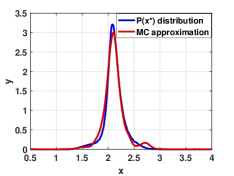
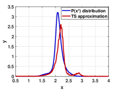
We demonstrate the superiority in Figure 2. We denote the GMD estimated from 50,000 TS samples of a full GP posterior on a 1$d$ function as our reference $p(\boldsymbol{x}^{*})$, showing as blue lines in Figure 2a and Figure 2b. We give the same running time ($0.5s$) to TS and MC approaches to approximate the reference $p(\boldsymbol{x}^{*})$ respectively, showing as red lines in Figure 2a and Figure 2b. We can see that our MC approach successfully approximate the reference $p(\boldsymbol{x}^{*})$ while TS is not desirable.

3.3 Expected improvement acquisition function as a proxy

To further reduce the computation, we propose to use EI function as a proxy for $q(\boldsymbol{x}^{*})$. This choice is reasonable in sense that they both measure the belief about the location of the global maximum, and it can be seen from Figure 1d that the GMD of full GP and the EI resembles closely. In this setting of RSSGP, we can expect similar performance of capturing $q(\boldsymbol{x}^{*})$ information compare to the example showing in Figure 1c. Since EI is a function, so we shall firstly use histogram based method to acquire the PMF of EI and then to calculate the entropy. Although it may inaccurate, in most of the cases we find it to work satisfactorily.

We use stochastic gradient descent to optimize Eq.(11) although alternatives are available. The proposed method is described in Algorithm 1.

Algorithm 1 Regularised Sparse Spectrum Gaussian Process for Bayesian Optimization

1:$\mathbf{for}$ $n$ = $1$, $2$,…$t$ $\mathbf{do}$

2:     Optimize Eq.(11) to obtain hyerpararameters and optimal features

3:     Fit the data $\mathcal{D}_{t}$ with RSSGP,

4:   Suggest the next point $\boldsymbol{x}_{t+1}$ by maximising $\boldsymbol{x}_{t+1}$ = $\text{argmax}\alpha_{EI}(\boldsymbol{x}|\mathcal{D})$,

5:     Evaluate the function value $y_{t+1}$,

6:     Augment the observations$\mathcal{D}_{t}=\mathcal{D}_{t}\cup(\boldsymbol{x}_{t+1},y_{t+1})$.

7: $\mathbf{end}$ $\mathbf{for}$

4 Experiments

In this section, we evaluate our methods on optimizing benchmark functions, an alloy design problem and hyperparameter tuning of machine learning problems using transfer learning. We compare the following probabilistic models used for Bayesian optimization:

• Full Gaussian process (Full GP)

• Sparse spectrum Gaussian process (SSGP)

• Our method 1: Regularized sparse spectrum Gaussian process with MC estimation for $q(\boldsymbol{x}^{*})$ (RSSGP-MC)

• Our method 2: Regularized sparse spectrum Gaussian process with EI approximation for $q(\boldsymbol{x}^{*})$ (RSSGP-EI)

• Variational Fourier features for Gaussian process using additive kernel (VFF-AK)

• Variational Fourier features for Gaussian process using Kronecker kernel (VFF-KK)

In all settings, we use EI as the acquisition function in Bayesian optimization and use the optimiser DIRECT [25] to maximize the EI function. We include both RSSGP-MC and RSSGP-EI in synthetic experiments. We later only use RSSGP-EI due to its computational advantage and the similar performance with RSSGP-MC. Given $d$-dimensional optimization problems and $m$ frequencies, the size of inducing variables would be $(2m)*d$ for VFF-AK and $(2m)^{d}$ for VFF-KK [17]. Thus, VFF-KK becomes almost prohibitively expensive for $d>2$ and a large $m$.

(a) 2d-Ackley

(b) 6d-Hartmann

Figure 3: Simple regret vs iterations for the optimization of (a) 2$d$ Ackley and (b) 6$d$ Hartmann. The plots show the mean of minimum reached and its standard error at each iteration.

4.1 Optimizing benchmark functions

We test on the following two benchmark functions:

• 2$d$ Ackley function. Its global minimum is $f(\boldsymbol{x}^{\ast})=0$ and the search space is $[-10,10]^{2}$;

• 6$d$ Hartmann function. Its global minimum is $f(\boldsymbol{x}^{\ast})=-3.32237$ and the search space is $[0,1]^{6}$;

We run each method for 50 trials with different initializations and report the average simple regret along with standard errors. The simple regret is defined as $r_{t}=f(\boldsymbol{x}^{*})-f(\boldsymbol{x}^{+})$, where $f(\boldsymbol{x}^{*})$ is the global maximum and $f(\boldsymbol{x}^{+})=\max{}_{\boldsymbol{x}\in\{\boldsymbol{x}_{1:t}\}}f(\boldsymbol{x})$ is the best value till iteration $t$. In terms of kernel parameters, we use the isotropic length scale, $\rho_{l}=0.5,\forall l$, signal variance$\sigma_{f}^{2}=2$, and noise variance $\sigma_{n}^{2}=(0.01)^{2}$. We empirically find that the proposed algorithms perform well when the regularization term has the more or less scale with the log marginal likelihood. Therefore, we set the trade-off parameter $\lambda=10$ for all of our methods.

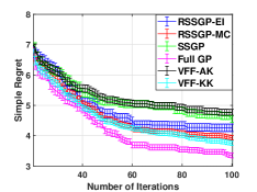
For the 2$d$ Ackley function, we start with 20 initial observations and use 20 frequencies in all spectrum GP models. The experimental result is shown in Figure 3a. BO using FullGP performs best. Both of our approaches (e.g., RSSGP-MC and RSSGP-EI) perform better than SSGP. RSSGP-EI performs slightly worse than RSSGP-MC since it only provides a rough approximation to the true global maximum distribution but holds simplicity. VFF-KK performs well in a low dimensional problem whilst VFF-AK performs worst. The use of additive kernel which does not capture the correlation between dimensions may cause a bad performance of VFF-AK.

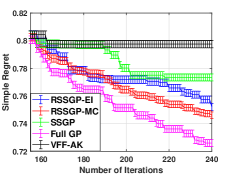
For the 6$d$ Hartmann function, we start with 150 initial observations and use 50 frequency features in all spectrum GP models. Similar results as the 2$d$ Ackley function can be seen in Figure 3b. We did not run VFF-KK on this 6$d$ function optimization due to a huge size of inducing variables mentioned before.

Figure 4: Alloy optimization-FCC at 15-dimensions.

4.2 Alloy optimization

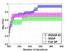
In the joint project with our metallurgist collaborators, we aim to design an alloy with a micro-structure that contains as much fraction of FCC phase as possible. We use a thermodynamic simulator called ThermoCalc [26]. Given a composition of an alloy, the simulator can compute thermodynamic equilibrium and predict the micro-structure of the resultant alloy using CALPHAD [27] methodology. In this experiment, the search space is a 15 dimensional combination of the elements: Fe, Ni, Cr, Ti, Co, Al, Mn, Cu, Si, Nb, Mo, W, Ta, C, N. For each composition, ThermoCalc provides the amount of FCC in terms of volume fraction. The best value of volume fraction is 1. Since ThermoCalc takes around 10 minutes per composition to compute volume fraction, it fits perfectly in our notion of semi-expensive functions. We use 500 initial points and 50 sparse features and run 5 different trials with different initial points. The results in Figure 4 shows BO with RSSGP-EI performs the best over all three methods. We found that the covariance matrix of the full GP easily became ill-conditioned in the presence of a large number of observations, and hence, fails to be inverted properly, being ended up harming the BO.

(a) LiverDisorders as Target

(b) Madelon as Target

(c) Mushroom as Target

(d) BreastCancer as Target

Figure 5: Hyperparameters tuning for SVM classifier by transfer learning. The plots show the maximal accuracy reached till the current iteration by RSSGP-EI (blue), SSGP (green) and by FullGP (mauve). Error bar indicates the standard error.

4.3 Transfer learning on hyperparameter tuning

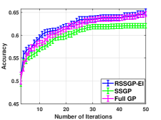
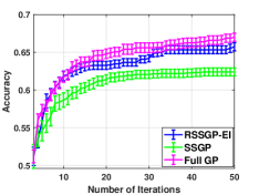
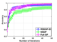
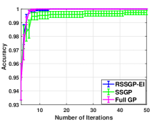
Transfer learning in the context of Bayesian optimization pools together observations from the sources and the target to build a covariance matrix in the GP. In this case when the number of sources is large or/and the number of existing observations per source is large, the resultant covariance matrix can be quite huge, demanding a sparse approximation. We conduct experiments for tuning hyperparameters of Support vector machine (SVM) classifier in a transfer learning setting. We use the datasets: LiverDisorders, Madelon, Mushroom and BreastCancer from UCI repository [28] and construct four transfer learning scenarios. For each scenario, we use 3 out of 4 datasets as the source tasks, and the rest one as the target task. We randomly generate 900 samples of hyperparameters and the corresponding accuracy values from each source task. We also randomly generate 3 initial samples from the target task. As a result, we have 2703 initial observations to build the combined covariance matrix. Following the framework [10] where source points are considered as noisy observations for the target function, we add a higher noise variance (3 times of that in target observations) to 2700 source observations . This allows us to use the same covariance function to capture the similarity between the observations from both source and target tasks. We optimize two hyperparameters in SVM which are the cost parameter ($C$) and the width of the RBF kernel ($\gamma$). The search bounds for the two hyperparameters are $C$ =$10^{\lambda}$ where $\lambda\in[-3,3]$, and $\gamma=10^{\omega}$ with $\omega\in[-3,0]$, respectively, and we optimize $\lambda$ and $\omega$. We run each scenario 30 trials with different initializations. The results are showed in Figure 5. We can see that in all scenarios BO with RSSGP-EI outperforms the naive SSGP. We note that the covariance matrix of full GP for transfer learning tasks does not always suffer from ill-conditioning since the source observations have a higher noise. Therefore, we can see BO with the full GP works well from the results.

5 Conclusion

In this paper we proposed a new regularized sparse spectrum Gaussian process method to make it more suitable for Bayesian optimization applications. The original formulation results in an over-confident GP. BO using such an over-confident GP may fare poorly as the correct uncertainty prediction is crucial for the success of BO. We propose a modification to the original marginal likelihood based estimation by adding the entropy of the global maximum distribution induced by the posterior GP as a regularizer. By maximizing the entropy of that distribution along with the marginal likelihood, we aim to obtain a sparse approximation which is more aligned with the goal of BO. We show that an efficient formulation can be obtained by using a sequential Monte Carlo approach to approximate the global maximum distribution. We also experimented with the expected improvement acquisition function as a proxy to the global maximum distribution. Experiments on benchmark functions and two real world problems show superiority of our approach over the vanilla SSGP method at all times and even better than the usual full GP based approach at certain scenarios.

References

- [1] D. R. Jones, M. Schonlau, W. J. Welch, Efficient global optimization of expensive black-box functions, Journal of Global optimization 13 (4) (1998) 455–492.
- [2] E. Brochu, V. M. Cora, N. De Freitas, A tutorial on bayesian optimization of expensive cost functions, arXiv preprint arXiv:1012.2599.
- [3] B. Shahriari, K. Swersky, Z. Wang, R. P. Adams, N. De Freitas, Taking the human out of the loop: A review of bayesian optimization, Proceedings of the IEEE 104 (1) (2015) 148–175.
- [4] A. Yang, C. Li, S. Rana, S. Gupta, S. Venkatesh, Efficient bayesian optimisation using derivative meta-model, in: The 15th Pacific Rim International Conference on Artificial Intelligence, 2018, 2018.
- [5] J. Snoek, H. Larochelle, R. P. Adams, Practical bayesian optimization of machine learning algorithms, in: NeurIPS, 2012, pp. 2951–2959.
- [6] J. T. Springenberg, A. Klein, S. Falkner, F. Hutter, Bayesian optimization with robust bayesian neural networks, in: NeurIPS, 2016, pp. 4134–4142.
- [7] C. Li, D. R. de Celis Leal, S. Rana, S. Gupta, A. Sutti, S. Greenhill, T. Slezak, M. Height, S. Venkatesh, Rapid bayesian optimisation for synthesis of short polymer fiber materials, Scientific Reports 7.
- [8] S. J. Pan, Q. Yang, A survey on transfer learning, IEEE Transactions on knowledge and data engineering 22 (10) (2009) 1345–1359.
- [9] M. Long, J. Wang, G. Ding, J. Sun, P. S. Yu, Transfer feature learning with joint distribution adaptation, in: Proceedings of the IEEE international conference on computer vision, 2013, pp. 2200–2207.
- [10] T. T. Joy, S. Rana, S. Gupta, S. Venkatesh, A flexible transfer learning framework for bayesian optimization with convergence guarantee, Expert Systems with Applications 115 (2019) 656–672.
- [11] J. Snoek, O. Rippel, K. Swersky, R. Kiros, N. Satish, N. Sundaram, M. Patwary, M. Prabhat, R. Adams, Scalable bayesian optimization using deep neural networks, in: ICML, 2015, pp. 2171–2180.
- [12] F. Hutter, H. H. Hoos, K. Leyton-Brown, Sequential model-based optimization for general algorithm configuration, in: LION, Springer, 2011, pp. 507–523.
- [13] E. Snelson, Z. Ghahramani, Sparse gaussian processes using pseudo-inputs, in: NeurIPS, 2006, pp. 1257–1264.
- [14] A. Yang, C. Li, S. Rana, S. Gupta, S. Venkatesh, Sparse approximation for gaussian process with derivative observations, in: Australasian Joint Conference on Artificial Intelligence, Springer, 2018, pp. 507–518.
- [15] M. Titsias, Variational learning of inducing variables in sparse gaussian processes, in: Artificial Intelligence and Statistics, 2009, pp. 567–574.
- [16] M. Lazaro Gredilla, J. Quinonero Candela, C. E. Rasmussen, A. R. Figueiras Vidal, et al., Sparse spectrum gaussian process regression, Journal of Machine Learning Research 11 (Jun) (2010) 1865–1881.
- [17] J. Hensman, N. Durrande, A. Solin, et al., Variational fourier features for gaussian processes., Journal of Machine Learning Research 18 (151) (2017) 1–151.
- [18] P. Hennig, C. J. Schuler, Entropy search for information-efficient global optimization, Journal of Machine Learning Research 13 (Jun) (2012) 1809–1837.
- [19] J. M. Hernández, M. W. Hoffman, Z. Ghahramani, Predictive entropy search for efficient global optimization of black-box functions, in: NeurIPS, 2014, pp. 918–926.
- [20] C. E. Rasmussen, C. K. Williams, Gaussian processes for machine learning, Vol. 1, MIT press Cambridge, 2006.
- [21] J. Mockus, Application of bayesian approach to numerical methods of global and stochastic optimization, Journal of Global Optimization 4 (4) (1994) 347–365.
- [22] S. Bochner, Lectures on Fourier integrals, Princeton University Press, 1959.
- [23] H. Bijl, T. B. Schön, J.-W. van Wingerden, M. Verhaegen, A sequential monte carlo approach to thompson sampling for bayesian optimization, arXiv preprint arXiv:1604.00169.
- [24] G. Kitagawa, Monte carlo filter and smoother for non-gaussian nonlinear state space models, Journal of computational and graphical statistics 5 (1) (1996) 1–25.
- [25] D. E. Finkel, Direct optimization algorithm user guide, CRSC.
- [26] J.-O. Andersson, T. Helander, L. Höglund, P. Shi, B. Sundman, Thermo-calc & dictra, computational tools for materials science, Calphad 26 (2) (2002) 273–312.
- [27] N. Saunders, A. P. Miodownik, CALPHAD (calculation of phase diagrams): a comprehensive guide, Vol. 1, Elsevier, 1998.
-
[28]
D. Dheeru, E. Karra Taniskidou, UCI
machine learning repository (2017).
URL http://archive.ics.uci.edu/ml