A Performance and Cost Assessment of Machine Learning Interatomic Potentials

Abstract

Machine learning of the quantitative relationship between local environment descriptors and the potential energy surface of a system of atoms has emerged as a new frontier in the development of interatomic potentials (IAPs). Here, we present a comprehensive evaluation of ML-IAPs based on four local environment descriptors — Behler-Parrinello symmetry functions, smooth overlap of atomic positions (SOAP), the Spectral Neighbor Analysis Potential (SNAP) bispectrum components, and moment tensors — using a diverse data set generated using high-throughput density functional theory (DFT) calculations. The data set comprising bcc (Li, Mo) and fcc (Cu, Ni) metals and diamond group IV semiconductors (Si, Ge) is chosen to span a range of crystal structures and bonding. All descriptors studied show excellent performance in predicting energies and forces far surpassing that of classical IAPs, as well as predicting properties such as elastic constants and phonon dispersion curves. We observe a general trade-off between accuracy and the degrees of freedom of each model, and consequently computational cost. We will discuss these trade-offs in the context of model selection for molecular dynamics and other applications.

I Introduction

A fundamental input for atomistic simulations of materials is a description of the potential energy surface (PES) as a function of atomic positions. While quantum mechanics-based descriptions, such as those based on Kohn-Sham density functional theory (DFT)Kohn and Sham (1965); Sham and Schlüter (1983), are accurate and transferable across chemistries, their high cost and poor scaling (typically $O(n_{e}^{3})$ or higher, where $n_{e}$ is the number of electrons)Zhang et al. (2011, 2009); Ji et al. (2013) limits simulations to $\sim$ 1000 atoms and hundreds of picoseconds. Hence, large-scale and long-time simulations traditionally rely on interatomic potentials (IAPs), which to date are in most cases empirical parameterizations of the PES based on physical functional forms that depend only on the atomic degrees of freedom.Rappe et al. (1992); Mayo et al. (1990); Van Duin et al. (2001) IAPs gain linear scaling with respect to the number of atoms at the cost of accuracy and transferability.

In recent years, a modern alternative has emerged in the form of machine-learned IAPs (ML-IAPs), where the PES is described as a function of local environment descriptors that are invariant to translation, rotation and permutation of homonuclear atomsBehler (2016); Bartók et al. (2013). Examples of such potentials include the high-dimensional neural network potential (NNP)Behler and Parrinello (2007); Behler (2011a), the Gaussian approximation potential (GAP)Bartók et al. (2013); Szlachta et al. (2014); Dragoni et al. (2018), the Spectral Neighbor Analysis Potential (SNAP)Thompson et al. (2015); Chen et al. (2017); Li et al. (2018); Deng et al. (2019), moment tensor potentials (MTP),Shapeev (2016); Podryabinkin and Shapeev (2017); Gubaev et al. (2019) among othersBotu and Ramprasad (2015a, b); Botu et al. (2017); Kruglov et al. (2017); Li et al. (2015); Chmiela et al. (2017); Brockherde et al. (2017); Rupp (2015); Huang et al. (2019); Shapeev (2017). A typical approach to training such potentials involves the generation of a sufficiently large and diverse data set of atomic configurations with corresponding energies, forces and stresses from DFT calculations, which are then used in the training of the ML-IAP based on one or several target metrics, such as minimizing the mean absolute or squared errors in predicted energies, forces, stresses or derived properties (e.g. elastic constants). ML-IAPs have been shown to be a remarkable improvement over traditional IAPs, in general, achieving near-DFT accuracy in predicting energies and forces across diverse chemistries and atomic configurations. Nevertheless, a critical gap that remains is a rigorous assessment of the relative strengths and weaknesses of ML-IAPs across a standardized data set, similar to what has been done for classical IAPs.Balamane et al. (1992); O’connor and Biersack (1986); Godet et al. (2003).

In this work, we present a comprehensive performance comparison of four major ML-IAPs — GAP, MTP, NNP and SNAP. The four IAPs were evaluated in terms of their accuracy in reproducing DFT energies and forces, as well as material properties such as the equations of state, lattice parameter and elastic constants. An attempt was also made to assess the training data requirements of each ML-IAP and the relative computational cost based on the best-available current implementations. To ensure a fair comparison, standardized DFT data sets of six elements (Li, Mo, Cu, Ni, Si and Ge) with the same training/test sampling and similar fitting approaches was used. The elements were chosen to span diverse chemistries and bonding, e.g., bcc and fcc metals, main group and transition metals, and group IV semiconductors.

II Methods

II.1 Machine learning interatomic potentials

The four ML-IAPs investigated in this work have already been extensively discussed in previous works and reviewsBehler and Parrinello (2007); Behler (2016, 2011a, 2015, 2017); Bartók et al. (2013); Szlachta et al. (2014); Dragoni et al. (2018); Mocanu et al. (2018); Thompson et al. (2015); Chen et al. (2017); Li et al. (2018); Deng et al. (2019); Wood et al. (2019); Shapeev (2016); Podryabinkin and Shapeev (2017); Gubaev et al. (2019). All ML-IAPs express the potential energy as a sum of atomic energies that are a function of the local environment around each atom, but differ in the descriptors for these local environments and the ML approach/functional expression used to map the descriptors to the potential energy. The detailed formalism of all four ML-IAPs are provided in the Supplementary Information. Here, only a concise summary of the key concepts and model parameters behind the ML-IAPs in chronological order of development, is provided to aid the reader in following the remainder of this paper.

1. High-dimensional neural network potential (NNP). The NNP uses atom-centered symmetry functions (ACSF)Behler (2011b) to represent the atomic local environments and fully connected neural networks to describe the PES with respect to symmetry functionsBehler and Parrinello (2007); Behler (2011a). A separate neural network is used for each atom. The neural network is defined by the number of hidden layers and the nodes in each layer, while the descriptor space is given by the following symmetry functions:

   $$G_{i}^{\rm atom,\rm rad} = \sum_{j\neq i}^{N_{\rm atom}}e^{-\eta(R_{ij}-R_{s})^{2}}\cdot f_{c}(R_{ij}),$$ (1)

   $$G_{i}^{\rm atom,\rm ang} = 2^{1-\zeta}\sum_{j,k\neq i}^{N_{\rm atom}}(1+\lambda\cos\theta_{ijk})^{\zeta}\cdot e^{-\eta^{\prime}(R_{ij}^{2}+R_{ik}^{2}+R_{jk}^{2})}\cdot f_{c}(R_{ij})\cdot f_{c}(R_{ik})\cdot f_{c}(R_{jk}),$$ (2)

   where $R_{ij}$ is the distance between atom $i$ and neighbor atom $j$, $\eta$ is the width of the Gaussian and $R_{s}$ is the position shift over all neighboring atoms within the cutoff radius $R_{c}$, $\eta^{\prime}$ is the width of the Gaussian basis and $\zeta$ controls the angular resolution. $f_{c}(R_{ij})$ is a cutoff function, defined as follows:

   $$f_{c}(R_{ij})=\begin{cases}\ 0.5\cdot[\cos{(\frac{\pi R_{ij}}{R_{c}})}+1],&\text{for }R_{ij}\leq R_{c}\\ \ 0.0,&\text{for }R_{ij}>R_{c}.\end{cases}$$ (3)

   These hyperparameters were optimized to minimize the mean absolute errors of energies and forces for each chemistry. The NNP model has shown great performance for SiBehler and Parrinello (2007), TiO2Artrith and Urban (2016), waterMorawietz et al. (2016) and solid-liquid interfacesQuaranta et al. (2017), metal-organic frameworksEckhoff and Behler (2019), and has been extended to incorporate long-range electrostatics for ionic systems such as ZnOArtrith et al. (2011) and Li3PO4Li et al. (2017).

2. Gaussian Approximation Potential (GAP). The GAP calculates the similarity between atomic configurations based on a smooth-overlap of atomic positions (SOAP)Bartók et al. (2010, 2013) kernel, which is then used in a Gaussian process model. In SOAP, the Gaussian-smeared atomic neighbor densities $\rho_{i}(\bm{R})$ are expanded in spherical harmonics as follows:

   $$\rho_{i}(\bm{R})=\sum_{j}f_{c}(R_{ij})\cdot\exp(-\frac{|\bm{R}-\bm{R}_{ij}|^{2}}{2\sigma_{\rm atom}^{2}})=\sum_{nlm}c_{nlm}\ g_{n}(R)Y_{lm}(\hat{\bm{R}}),$$ (4)

   The spherical power spectrum vector, which is in turn the square of expansion coefficients,

   $$p_{n_{1}n_{2}l}(\bm{R}_{i})=\sum_{m=-l}^{l}c_{n_{1}lm}^{\ast}c_{n_{2}lm},$$ (5)

   can be used to construct the SOAP kernel while raised to a positive integer power $\zeta$ (which is 4 in present case) to accentuate the sensitivity of the kernelBartók et al. (2013),

   $$\bm{K}(\bm{R},\bm{R^{\prime}})=\sum_{n_{1}n_{2}l}(p_{n_{1}n_{2}l}(\bm{R})p_{n_{1}n_{2}l}(\bm{R^{\prime}}))^{\zeta},$$ (6)

   In the above equations, $\sigma_{\rm atom}$ is a smoothness controlling the Gaussian smearing, and $n_{\text{max}}$ and $l_{\text{max}}$ determine the maximum powers for radial components and angular components in spherical harmonics expansion, respectivelyBartók et al. (2013). These hyperparameters, as well as the number of reference atomic configurations used in Gaussian process, are optimized in the fitting procedure to obtain optimal performance. The GAP has been developed for transition metalsSzlachta et al. (2014); Dragoni et al. (2018), main group elementsDeringer et al. (2018a); Deringer and Csányi (2017); Rowe et al. (2018), diamond semiconductorsBartók et al. (2018); Deringer et al. (2018b) as well as multi-component systemsMocanu et al. (2018).

3. Spectral Neighbor Analysis Potential (SNAP). The SNAP uses the coefficients of the bispectrum of the atomic neighbor density functionsBartók et al. (2013) as descriptors. In the original formulation of SNAP, a linear model between energies and bispectrum components is assumedThompson et al. (2015). Recently, a quadratic model (denoted as qSNAP in this work)Wood and Thompson (2018) has been developed, which extends the linear SNAP energy model to include all distinct pairwise products of bispectrum components. In this work, both linear and quadratic SNAP models were investigated. The key hyperparameters influencing model performance are the cutoff radius and $J_{\text{max}}$, which limits the indices $j_{1}$, $j_{2}$, $j$ in Clebsch-Gordan coupling coefficients $H\begin{subarray}{c}jmm\prime\\ j_{1}m_{1}m_{1}^{\prime}\\ j_{2}m_{2}m_{2}^{\prime}\end{subarray}$ in construction of the bispectrum components:

   $$\begin{split}B_{j_{1},j_{2},j}&=\sum_{m_{1},m_{1}^{\prime}=-j_{1}}^{j_{1}}\sum_{m_{2},m_{2}^{\prime}=-j_{2}}^{j_{2}}\sum_{m,m^{\prime}=-j}^{j}(u_{m,m^{\prime}}^{j})^{\ast}\\ &\times H\begin{subarray}{c}jmm\prime\\ j_{1}m_{1}m_{1}^{\prime}\\ j_{2}m_{2}m_{2}^{\prime}\end{subarray}u_{m_{1},m_{1}^{\prime}}^{j_{1}}u_{m_{2},m_{2}^{\prime}}^{j_{2}},\end{split}$$ (7)

   where $u_{m,m^{\prime}}^{j}$ are coefficients in 4-dimensional hyper-spherical harmonics expansion of neighbor density function:

   $$\rho_{i}(\textbf{R})=\sum_{j=0}^{\infty}\sum_{m,m^{\prime}=-j}^{j}u_{m,m^{\prime}}^{j}U_{m,m^{\prime}}^{j},$$ (8)

   The SNAP model as well as qSNAP model has demonstrated great success in transition metalsThompson et al. (2015); Chen et al. (2017); Li et al. (2018); Wood and Thompson (2018) as well as binary systemsLi et al. (2018); Deng et al. (2019); Wood et al. (2019).

4. Moment Tensor Potential (MTP). The MTPShapeev (2016) devises rotationally-covariant tensors

   $$M_{\mu,\nu}(\bm{R})=\sum_{j}f_{\mu}(R_{ij})\ \underbrace{\bm{R}_{ij}\otimes\dots\otimes\bm{R}_{ij}}_{\nu\ times},$$ (9)

   to describe the atomic local environments. Here $f_{\mu}$ are the radial functions, and $\bm{R}_{ij}\otimes\dots\otimes\bm{R}_{ij}$ are tensors of rank $\nu$ encoding angular information about the atomic environment. The rank $\nu$ can be large enough to approximate any arbitrary interactions. MTP then contracts these tensors to a scalar yields rotationally-invariant basis functions, and applies linear regression to correlate the energies with the basis functions. The performance of MTP is controlled by the polynomial power-like metric, which defines what tensors and how many times are contracted. The MTP model has been successfully applied to metalsShapeev (2016); Podryabinkin and Shapeev (2017); Novoselov et al. (2019), boronPodryabinkin et al. (2019), binary and ternary alloysGubaev et al. (2019) as well as gas-phase chemical reactionsNovikov et al. (2018).

II.2 DFT Data Sets

A comprehensive DFT data set was generated for six elements - Li, Mo, Ni, Cu, Si and Ge. These elements were chosen to span a variety of chemistries (main group metal, transition metal and semiconductor), crystal structures (bcc, fcc, and diamond) and bonding types (metallic and covalent). For each element, we generated a set of structures with diverse coverage of atomic local environment space, as follows:

1. The ground-state crystal for each element.

2. Strained structures constructed by applying strains of $-10\%$ to 10% at 2% intervals to the bulk supercell in six different modes, as described in the work by de Jong et al. (2015). The supercells used are the $3\times 3\times 3$, $3\times 3\times 3$ and $2\times 2\times 2$ of the conventional bcc, fcc and diamond unit cells, respectively.

3. Slab structures up to a maximum Miller index of three, including (100), (110), (111), (210), (211), (310), (311), (320), (321), (322), (331), and (332), as obtained from the Crystalium databaseTran et al. (2016); http://crystalium.materialsvirtuallab.org (2016).

4. NVT ab initio molecular dynamics (AIMD) simulations of the bulk supercells (similar to those in (2)) performed at 300 K and $0.5\times$, $0.9\times$, $1.5\times$, $2.0\times$ of the melting point of each element. A total of 20 snapshots were obtained from each AIMD simulation at an interval of 0.1 ps, unless otherwise stated.

5. NVT AIMD simulations of the bulk supercells (similar to those in (2)) with a single vacancy performed at 300 K and $2.0\times$ of the melting point of each element. A total of 40 snapshots were obtained from each AIMD simulation at an interval of 0.1 ps, unless otherwise stated.

All DFT calculations were carried out using the Vienna ab initio simulation package (VASP)Kresse and Furthmüller (1996) version 5.4.1 within the projector augmented wave approachBlöchl (1994). The Perdew-Burke-Ernzerhof (PBE) generalized gradient approximation (GGA)Perdew et al. (1996) was adopted for the exchange-correlation functional. The kinetic-energy cutoff was set to 520 eV and the $k$-point mesh was $4\times 4\times 4$ for the Mo, Ni, Cu, Si and Ge supercells, and $3\times 3\times 3$ for the Li supercells. The electronic energy and atomic force components were converged to within $10^{-5}$ eV and 0.02 eV/Å, respectively, in line with previous worksChen et al. (2017); Li et al. (2018). The AIMD simulations were carried out with a single $\Gamma$ k point and were non-spin-polarized, but static calculations using the same parameters as the rest of the data were carried out on the snapshots to obtain consistent energies and forces. All structure manipulations and analyses of DFT computations were carried out using Python Materials Genomics (Pymatgen)Ong et al. (2013) library, and the automation of calculations was performed using the Fireworks softwareJain et al. (2015).

II.3 Optimization scheme

Figure 1: Machine-learning interatomic potential development workflow.

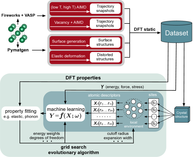
Figure 1 provides an overview of the general data generation and potential development scheme. The training data set was first generated via DFT static calculations on the four categories of structures. The optimization procedure comprised two loops. In the inner loop, sampled structures in the database were transformed into atomic descriptors (e.g., bispectrum components for SNAP and symmetry functions for NNP), which were then fed into the corresponding ML model together with the DFT energies, forces, and stresses as the targets of training. The data was apportioned into training and test sets with a 90:10 split. The parameters of the ML models were optimized during the training process. In the outer loop, the ML model trained in the inner loop was used to predict basic material properties (e.g., elastic tensors), and the differences between the predicted and reference values were then used to determine the optimal hyperparameters for each ML-IAPs. In this work, we adopted a combination of the grid search algorithm and differential evolution algorithm to perform hyperparameters optimization for different ML-IAPs.

II.4 Data and code availability

To facilitate the reuse and reproduction of our results, the code, data and optimized ML models in this work are published open-source on Github (https://github.com/materialsvirtuallab/mlearn). The code includes high-level Python interfaces for ML-IAPs development as well as LAMMPS material properties calculators.

III Results

III.1 Optimized model parameters

The optimized coefficients and hyperparameters for each ML-IAP are reported in Supplementary Information (see Table S1–Table S10). Here, we will limit our discussions to a parameter that is common to all ML-IAPs - the cutoff radius - and present a convergence study of each ML-IAP with the number of degrees of freedom of the model.

The cutoff radius determines the maximum range of interatomic interactions, and hence, has a critical effect on the prediction performance of ML-IAPs. Table 1 provides the optimized cutoff radii of different ML-IAPs across different chemistries. Different ML-IAPs yield similar optimized cutoff radii for the same elemental system. The optimized cutoff radii are between the second nearest neighbor (2NN) and 3NN distance for fcc elements (Cu, Ni), between 3NN and 4NN distances for the bcc (Li, Mo) and diamond (Ge and Si) elements. These observations are consistent with those from previous traditional and ML IAP development efforts, where typically 2NN interactions are found to suffice for fcc metals,Lee et al. (2003); Foiles et al. (1986) while contributions from 3NN cannot be ignored for bcc metalsSong et al. (1999); Adams and Foiles (1990); Szlachta et al. (2014); Shapeev (2016); Podryabinkin and Shapeev (2017) and diamond systemsDe et al. (2016); Baskes et al. (1989).

	fcc		bcc		diamond
cutoff radius (Å)	Ni	Cu	Li	Mo	Si	Ge
GAP	3.9	3.9	4.8	5.2	5.4	5.4
MTP	4.0	3.9	5.1	5.2	4.7	5.1
NNP	3.9	4.1	5.2	5.2	5.2	5.6
SNAP	3.9	4.1	5.1	4.6	4.9	5.5
qSNAP	3.8	3.9	5.1	5.2	4.8	4.9

Table 1: Optimized cutoff radius for each element for each ML-IAP.

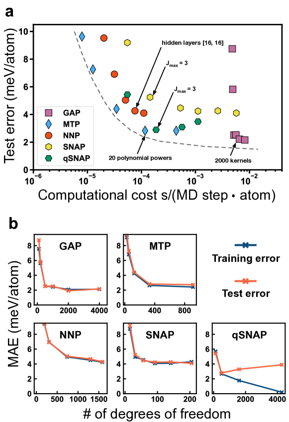
The number of degrees of freedom (DOF), e.g., the number of weights and biases for the NNP and number of representative points in GAP, has a strong effect on the accuracy and computational cost of each ML-IAP. Figure 2 illustrates the trade-off between computational cost and test error under varying DOFs for each fitted Mo ML-IAP. Similar results are obtained for other systems (see Figure S7–Figure S11). It should be noted that the relative computational costs are based on the most efficient available implementationsSingraber et al. (2019); Bartók et al. (2013); Shapeev (2016); Thompson et al. (2015); Wood and Thompson (2018) of each ML-IAP at this time in LAMMPSPlimpton (1995) and performed on a single CPU core of Intel i7-6850k 3.6 GHz with $18\times 18\times 18$ bulk supercell containing 23,328 atoms for Mo system. Future implementations may improve on these results. A Pareto frontier is drawn in Figure 2a to represent points at which better accuracy can only be attained at the price of greater computational costHuang et al. (2017), and the black arrows indicate “optimal” configurations for each model in terms of the trade-off between test error and computational cost. These “optimal” configurations were used for subsequent accuracy comparisons in energies, forces and properties. We find that the “optimal” MTP, NNP, SNAP and qSNAP models tend to be two orders of magnitude less computationally expensive than the “optimal” GAP model. The MTP models generally lie close to the Pareto frontier, exhibiting an excellent balance between model accuracy and computational efficiency. For the SNAP and qSNAP models, the descriptor space (i.e., bispectrum components) is determined by the parameter $J_{max}$. We find that the rate-limiting step is the calculation of bispectrum and the computation of quadratic terms in qSNAP has only a small effect on the computational cost.Wood and Thompson (2018). However, we find that the substantial expansion in the number of fitted coefficients in the qSNAP model results in a greater likelihood of over-fitting, especially for $J_{\text{max}}>3$ (see Figure 2b). For the GAP model, the computational cost is linearly related to the number of kernels used in Gaussian process regression.Szlachta et al. (2014).

Figure 2: (a) Test error versus computational cost for the Mo system. The black dash line indicates a Pareto frontier representing an optimal trade-off between accuracy and computational cost. Timings were performed by LAMMPS calculations on a single CPU core of Intel i7-6850k 3.6 GHz. Black arrows denote the “optimal” configuration for each ML-IAP that was used in subsequent comparisons. (b) Plots of the training and test errors versus the number of degrees of freedom for each ML-IAP.

III.2 Accuracy in energies and forces

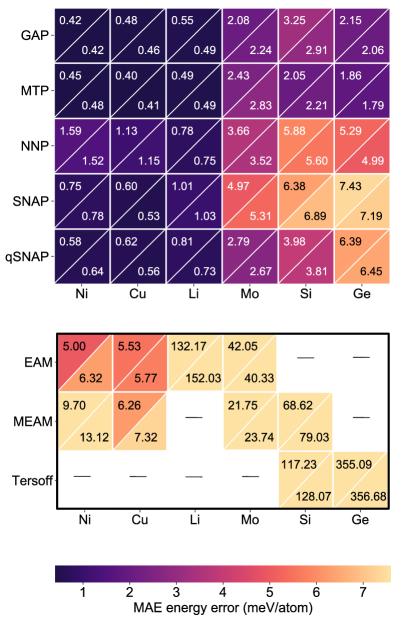
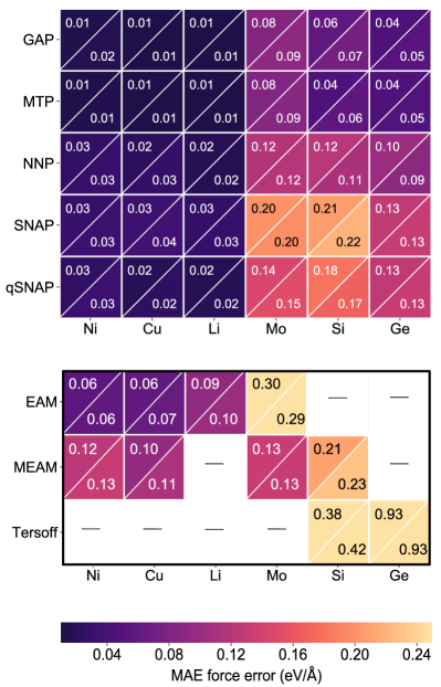
Figure 3 provides a comparison of the MAEs in energies and forces for the four ML-IAPs and best-available classical IAPs relative to DFT. All ML-IAPs show extremely good performance across all elements studied, achieving MAEs in energies and forces that are far lower than best-available traditional IAPs for each element. It should be noted that differences in MAEs between ML-IAPs are on the scale of meV atom^-1 in energies and 0.1 eV Å^-1 in forces; hence, any subsequent discussion on the relative performances of the ML-IAPs should be viewed in the context that even the largest differences in accuracy between the ML-IAPs are already close to the limits of DFT error. In all cases, the training and test errors are similar, indicating no over-fitting for the optimized ML-IAPs.

The GAP and MTP models generally have the lowest MAEs in energies and forces. The highest MAEs in energies are observed for the SNAP models and NNP models. It is well-known that neural network-based models often require larger data sets for best performance; previous NNP models have been trained on thousands or tens of thousands of structuresNguyen et al. (2018); Cheng et al. (2019), while only hundreds of structures are used in training the current ML-IAPs. Nevertheless, the NNP models still show surprisingly good performance for bcc systems. The qSNAP models’ performances are between those of the GAP and NNP. In general, the qSNAP models have moderately lower MAEs than the linear SNAP, though at the expense of a large expansion in the number of parameters.

In terms of chemistries, we find that the lowest MAEs in energies are observed for the fcc systems, followed by the bcc systems, and the highest MAEs are observed for the diamond systems. Very low MAEs in forces are observed across all ML IAPs for Cu, Ni and Li, while significantly higher MAEs in forces are observed for Mo, a metal with higher modulus and larger force distributions. Higher MAEs in forces are also observed for the diamond semiconductors. These trends are generally consistent across all ML-IAPs studied.

(a) Mean absolute errors in predicted energies

(b) Mean absolute errors in predicted forces

Figure 3: Mean absolute errors in (a) predicted energies (b) predicted forces for all four ML-IAPs as well as traditional IAPs (EAMZhou et al. (2004); Nichol and Ackland (2016), MEAMAsadi et al. (2015); Park et al. (2012); Lenosky et al. (2000), TersoffKumagai et al. (2007); Mahdizadeh and Akhlamadi (2017)). The upper left and lower right triangles within each cell represent training and test errors, respectively.

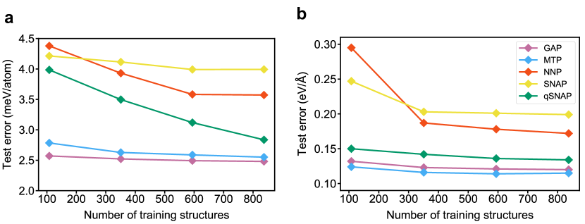
We have also performed a study of the convergence of the ML-IAPs with training data size using Mo as the benchmark system given that it is a bcc metal (for which traditional IAPs tend to perform poorly) with large force distributions. Here, the length of the AIMD simulations were increased four-fold, and more training structures were sampled at the same time interval. The convergence results are shown in Figure 4. While the prediction errors of all models decrease with increase in the number of training structures, the most substantial improvements in accuracy, especially in predicted energies, are observed for the NNP and qSNAP models. The SNAP Mo model appears to have converged in energy and force at a training data size of $\sim 600$ and $\sim 400$ structures, respectively. For the NNP, additional training structures offer modest improvements in force accuracy, but large improvements in energy accuracy. Indeed, it is possible that the NNP and qSNAP Mo models have not been converged with respect to accuracy in energies even at $\sim$ 800 training structures. We have not attempted to further converge these models in view of the computational expense involved.

Figure 4: MAE in predicted (a) energies (b) forces of the test set versus the size of the training data for the ML-IAP Mo models.

III.3 Accuracy in material properties

The accuracy in predicting basic material properties is critical for evaluating the performance of ML-IAPs. Here, we perform the climbing-image nudged elastic band (CI-NEB) methodHenkelman and Jónsson (2000) as well as molecular dynamics (MD) with ML-IAPs to obtain the cubic lattice parameter, elastic constants, migration energies and vacancy formation energies. The comparison of these predicted material properties with respect to the DFT values is provided in Table LABEL:table:elastic. The performances of all ML-IAPs are generally excellent, with lattice parameters within 0.1-2.0% of the DFT values and elastic constants that are typically within 10% of DFT values. It should be noted that the large percentage error in Li for elastic constants is due to the small reference values. The MTP, SNAP and qSNAP models perform well on elastic constants on fcc and bcc systems, but exhibit slightly higher prediction errors in the diamond systems. A possible explanation for the slightly poorer prediction of elastic constants of the NNP model could be the limitation of the size of training data, which restrict the potential of a fully connected neural network. However, it should be noted that despite the slightly higher prediction errors of elastic components for the NNP model, its prediction errors of Voigt-Reuss-Hill approximated bulk modulusHill (1952) across various elemental systems are in good agreement with DFT reference values.

In terms of diffusion properties, the GAP and MTP models perform well across different chemistries, with most of the prediction errors within 10% of DFT values, albeit with a moderate underestimate of the migration energy for diamond systems, in line with the previous studyBartók et al. (2018). While SNAP and qSNAP models show high accuracy in predicting diffusion properties for fcc systems, they considerably underestimate the vacancy formation energy as well as activation barrier for diamond systems. It is noteworthy that all ML-IAPs overestimate the migration energy of Mo system by more than 20%, which has also been observed in a previous workChen et al. (2017).

Table 2: Calculated cubic lattice parameter $a$, elastic constants ($c_{ij}$), Voigt-Reuss-Hill bulk modulus $B_{\text{VRH}}$, migration energy ($E_{m}$), vacancy formation energy ($E_{m}$) as well as activation barrier for vacancy diffusion ($E_{a}=E_{v}+E_{m}$) with DFT and the four ML-IAPs. Lowest absolute errors with respect to DFT for each property are bolded for ease of reference. Error percentages with respect to DFT values are shown in parentheses.

	DFT	GAP	MTP	NNP	SNAP	qSNAP
Ni
$a$ (Å)	3.508	3.523 (0.4%)	3.522 (0.4%)	3.523 (0.4%)	3.522 (0.4%)	3.521 (0.4%)
$c_{11}$ (GPa)	276	281 (1.8%)	284 (2.9%)	274 (-0.8%)	283 (2.5%)	267 ($-3.3\%$)
$c_{12}$ (GPa)	159	159 (0.0%)	172 (8.2%)	169 (6.3%)	168 (5.7%)	155 ($-2.5\%$)
$c_{44}$ (GPa)	132	126 ($-4.5\%$)	127 (-3.8%)	113 ($-14.4\%$)	129 (-2.3%)	125 ($-5.3\%$)
$\textit{B}_{\text{VRH}}$ (GPa)	198	200 (1.0%)	209 ($5.6\%$)	204 (3.0%)	206 (4.0%)	193 ($-2.5\%$)
$E_{v}$ (eV)	1.49	1.46 ($-2.0\%$)	1.43 ($-4.0\%$)	1.65 (10.7%)	1.47 (-1.3%)	1.47 (-1.3%)
$E_{m}$ (eV)	1.12	1.14 (1.8%)	1.11 ($-0.9\%$)	1.14 (1.8%)	1.12 (0.0%)	1.05 ($-6.3\%$)
$E_{a}$ (eV)	2.61	2.60 (-0.4%)	2.54 ($-2.7\%$)	2.79 (6.9%)	2.59 ($-0.8\%$)	2.52 ($-3.4\%$)
Cu
$a$ (Å)	3.621	3.634 (0.4%)	3.636 (0.4%)	3.637 (0.4%)	3.634 (0.4%)	3.636 (0.4%)
$c_{11}$ (GPa)	173	175 (1.2%)	177 (2.3%)	182 (5.2%)	178 (2.9%)	178 (2.9%)
$c_{12}$ (GPa)	133	120 ($-9.8\%$)	120 ($9.8\%$)	125 ($-6.0\%$)	126 ($-5.3\%$)	124 ($-6.8\%$)
$c_{44}$ (GPa)	88	82 ($-6.8\%$)	81 ($-8.0\%$)	76 ($-13.6\%$)	86 (-2.3%)	82 ($-6.8\%$)
$\textit{B}_{\text{VRH}}$ (GPa)	146	138 ($-5.5\%$)	139 ($-4.8\%$)	144 ($-1.4\%$)	143 (-2.1%)	142 ($-2.7\%$)
$E_{v}$ (eV)	1.15	1.05 ($-8.7\%$)	1.10 ($-4.3\%$)	1.23 (7.0%)	1.19 (3.5%)	1.15 (0.0%)
$E_{m}$ (eV)	0.79	0.76 ($-3.8\%$)	0.77 (-2.5%)	0.77 (-2.5%)	0.82 (3.8%)	0.74 ($-6.3\%$)
$E_{a}$ (eV)	1.94	1.81 ($-6.7\%$)	1.87 ($-3.6\%$)	2.00 (3.1%)	2.01 (3.6%)	1.89 (-2.6%)
Li
$a$ (Å)	3.427	3.450 (0.7%)	3.446 (0.6%)	3.434 (0.2%)	3.506 (2.3%)	3.469 (1.2%)
$c_{11}$ (GPa)	15	18 (20.0%)	14 ($-6.7\%$)	17 (13.3%)	18 (20.0%)	12 ($-20.0\%$)
$c_{12}$ (GPa)	13	14 (7.7%)	13 (0.0%)	12 (-7.7%)	7 ($-46.2\%$)	6 ($-53.8\%$)
$c_{44}$ (GPa)	11	12 (9.1%)	11 (0.0%)	12 (9.1%)	10 ($-9.1\%$)	11 (0.0%)
$\textit{B}_{\text{VRH}}$ (GPa)	14	15 (7.1%)	13 (-7.1%)	13 (-7.1%)	11 ($-21.4\%$)	8 ($-42.9\%$)
$E_{v}$ (eV)	0.62	0.56 ($-9.7\%$)	0.53 ($-14.5\%$)	0.50 ($-19.4\%$)	0.63 (1.6%)	0.58 ($-6.5\%$)
$E_{m}$ (eV)	0.06	0.06 (0.0%)	0.08 (33.3%)	0.05 ($-16.7\%$)	0.09 (50.0%)	0.09 (50.0%)
$E_{a}$ (eV)	0.68	0.62 ($-8.8\%$)	0.61 ($-10.3\%$)	0.55 ($-19.1\%$)	0.72 (5.9%)	0.67 (-1.5%)
Mo
$a$ (Å)	3.168	3.168 (0.0%)	3.169 (0.0%)	3.165 ($-0.1\%$)	3.169 (0.0%)	3.170 (0.1%)
$c_{11}$ (GPa)	472	481 (1.9%)	472 (0.0%)	441 ($-6.6\%$)	457 ($-3.2\%$)	436 ($-7.6\%$)
$c_{12}$ (GPa)	158	169 (7.0%)	154 (-2.5%)	192 (21.5%)	158 (0.0%)	166 (5.1%)
$c_{44}$ (GPa)	106	112 (5.7%)	103 ($-2.8\%$)	114 (7.5%)	109 (2.8%)	104 (-1.9%)
$\textit{B}_{\text{VRH}}$ (GPa)	263	271 (3.8%)	260 (-1.1%)	266 (1.1%)	258 ($-1.9\%$)	256 ($-2.7\%$)
$E_{v}$ (eV)	2.70	2.68 (-0.7%)	2.61 ($-3.3\%$)	2.94 (8.9%)	2.72 (0.7%)	2.79 (3.3%)
$E_{m}$ (eV)	1.22	1.60 (31.1%)	1.51 (23.8%)	1.59 (30.3%)	1.49 (22.1%)	1.50 (23.0%)
$E_{a}$ (eV)	3.92	4.28 (9.2%)	4.12 (5.1%)	4.53 (15.6%)	4.21 (7.4%)	4.29 (9.4%)
Si
$a$ (Å)	5.469	5.458 ($-0.2\%$)	5.465 (-0.1%)	5.459 ($-0.2\%$)	5.466 (0.1%)	5.464 (-0.1%)
$c_{11}$ (GPa)	156	168 (7.7%)	155 (-0.6%)	130 ($-9.7\%$)	141 ($-9.6\%$)	155 (-0.6%)
$c_{12}$ (GPa)	65	62 (-4.6%)	76 (16.9%)	77 ($18.5\%$)	61 ($-6.2\%$)	58 ($-10.8\%$)
$c_{44}$ (GPa)	76	69 ($-9.2\%$)	75 (-1.3%)	64 ($-15.8\%$)	71 ($-6.6\%$)	69 ($-9.2\%$)
$\textit{B}_{\text{VRH}}$ (GPa)	95	97 (2.1%)	102 (7.4%)	95 (0.0%)	93 ($-2.1\%$)	90 ($-5.3\%$)
$E_{v}$ (eV)	3.25	3.04 ($-6.5\%$)	3.11 (-4.3%)	2.63 ($-19.1\%$)	2.71 ($-16.6\%$)	2.37 ($-27.1\%$)
$E_{m}$ (eV)	0.21	0.21 (0.0%)	0.16 ($-23.8\%$)	0.25 (19.0%)	0.26 (23.8%)	0.20 ($-4.7\%$)
$E_{a}$ (eV)	3.46	3.25 ($-6.1\%$)	3.27 (-5.5%)	2.88 ($-16.8\%$)	2.97 ($-14.2\%$)	2.57 ($-25.7\%$)
Ge
$a$ (Å)	5.763	5.777 (0.2%)	5.770 (0.1%)	5.751 ($-0.5\%$)	5.773 (0.2%)	5.775 (0.2%)
$c_{11}$ (GPa)	116	127 (9.5%)	106 ($-8.6\%$)	101 ($-12.9\%$)	101 ($-12.9\%$)	121 (4.3%)
$c_{12}$ (GPa)	48	45 ($-6.3\%$)	54 (12.5%)	46 (-4.2%)	41 ($-14.6\%$)	43 ($-10.4\%$)
$c_{44}$ (GPa)	58	54 ($-6.9\%$)	55 (-5.2%)	46 ($-20.7\%$)	54 ($-6.9\%$)	50 ($-13.8\%$)
$\textit{B}_{\text{VRH}}$ (GPa)	71	72 (1.4%)	71 (0.0%)	69($-2.8\%$)	61 ($-14.1\%$)	69 ($-2.8\%$)
$E_{v}$ (eV)	2.19	2.10 (-4.1%)	1.98 ($-9.6\%$)	1.98 ($-9.6\%$)	1.77 ($-19.2\%$)	1.67 ($-23.7\%$)
$E_{m}$ (eV)	0.19	0.17 ($-10.5\%$)	0.17 ($-10.5\%$)	0.20 (5.3%)	0.28 (47.4%)	0.18 (-5.3%)
$E_{a}$ (eV)	2.38	2.27 (-4.6%)	2.15 ($-9.7\%$)	2.18 ($-8.4\%$)	2.05 ($-13.9$)	1.85 ($-22.3\%$)

III.4 Accuracy in equations of state

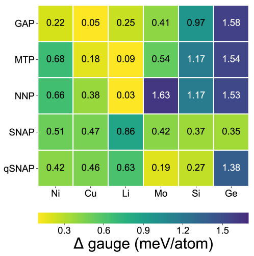
To provide an evaluation of the performance of ML-IAPs far from equilibrium, we have computed a pairwise comparison of the equation of state (EOS) curves for all elements studied using the $\Delta_{\text{EOS}}$ gauge of Lejaeghere et al.Lejaeghere et al. (2014); Csonka et al. (2009); Staroverov et al. (2004) The $\Delta_{\text{EOS}}$ gauge, which has been used to evaluate accuracy differences between DFT codes, is the root-mean-square difference between two EOS curves over a $\pm 6\%$ interval around the equilibrium volume, defined as follows:

$$\Delta_{\rm EOS}=\sqrt{\frac{\int_{0.94V_{0}}^{1.06V_{0}}[E^{\text{a}}(V)-E^{\text{b}}(V)]^{2}dV}{0.12V_{0}}}$$ (10)

where $E^{\text{a}}$ and $E^{\text{b}}$ denote energies computed using methods a and b, respectively.

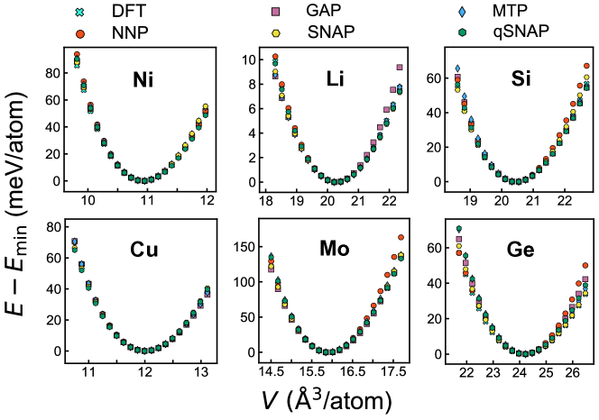
Figure 5(b) shows the $\Delta_{\text{EOS}}$ values of various machine learning models with respect to DFT reference data for different elemental systems as well as the EOS curves of these ML-IAPs. In all cases, the $\Delta_{\text{EOS}}$ for all ML-IAPs for all elements are within 2 meV/atom, which is the threshold for “indistinguishable EOS” previously used in evaluating different DFT codesLejaeghere et al. (2016). It is noteworthy that despite the relatively high prediction errors of SNAP models presented in Figure 3(a), they perform considerably better in predicting the EOS curves, with all the $\Delta_{\text{EOS}}$ lower than 1 meV/atom across different chemistries. The NNP models deviate slightly from DFT curves at both tensile and compressive strains for fcc systems, while for diamond systems, the deviation of the NNP models from DFT curve is comparable with those of GAP and MTP models, as evidenced in $\Delta$ gauge comparison. In general, it is more challenging to give highly accurate predictions of EOS in diamond system than in fcc and bcc systems. In addition to the DFT-level accuracy in equations of state prediction, the predicted phonon dispersion curves by all ML-IAPs investigated in this work are in excellent agreement with the DFT reference (see Figure S1–Figure S6 in the Supplementary Information).

(a) $\Delta$ gauge comparisons between ML-IAPs with respect to DFT

(b) Energy vs volume curves

Figure 5: Assessment of accuracy of ML-IAPs in predicting equation of state. (a) $\Delta$ gauge comparison provides quantitative estimate of deviation between the EOS curve from each ML-IAP with that of DFT. (b) EOS curves for all six elements using DFT and the four ML-IAPs.

III.5 Accuracy in molecular dynamics (MD) trajectories

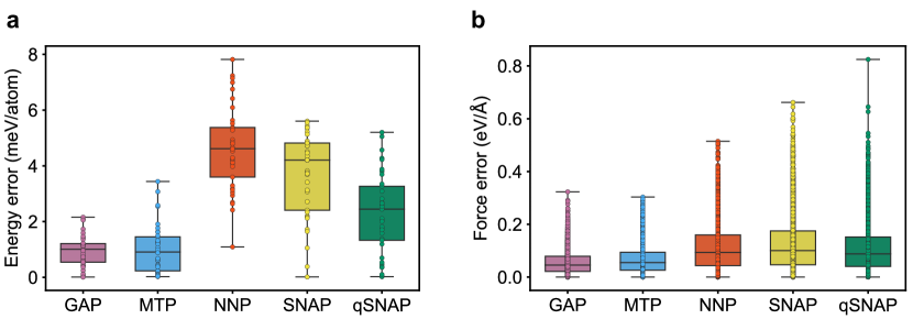
One of the principal applications of ML-IAPs is in molecular dynamics (MD) simulations. To assess the ability of the ML-IAPs to provide stable MD trajectories, we carried out $NVT$ MD simulations at 1,300 K ($0.5\times$ melting point) on a $3\times 3\times 3$ 54-atoms supercell of bulk Mo for 0.25 ns using LAMMPS with the different ML-IAPs. A total of 40 snapshots at an interval of 2.5 ps were then sampled from each MD trajectory, and DFT static calculations were performed on these snapshots. Figure 6 shows the distribution of the errors in the energies and forces of sampled structures. In line with the previous results, the GAP and MTP models generally exhibit smaller errors in the energies and forces than the NNP, SNAP and qSNAP models. The GAP model not only have the lowest median, but also the smallest interquartile range (IQR) in the errors in energies and forces. Somewhat interestingly, the NNP model has higher energy errors, but smaller force errors than SNAP and qSNAP. For consistency of comparison, all models shown here are the “optimal” models based on $\sim 100$ training structures. It is likely that a larger training set would improve the performance of the NNP and qSNAP models. (Figure 4).

Figure 6: Error distributions in (a) predicted energies (b) predicted forces for sampled structures from MD simulations using each ML-IAP. The rectangular box indicates the interquartile range (IQR), while the line within the box indicates the median.

III.6 Accuracy in polymorphic energy differences

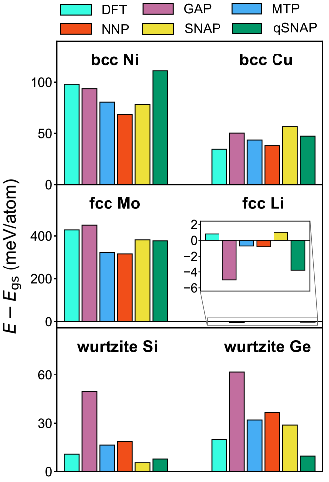
To evaluate the ability of the ML-IAPs to extrapolate to unseen data, we have computed the energy differences between the DFT ground state polymorph and a low-energy polymorph for each element, presented in Figure 7. The low-energy polymorphs correspond to the bcc, fcc, and wurtzite (hexagonal diamond) structures for the fcc, bcc, and diamond systems, respectively. It should be noted that only the ground state structures were used in training the ML-IAPs, and these low-energy polymorphs were not present in the training structures. Except for Li which has an extremely small energy difference between the fcc and bcc structures in DFT, all ML-IAPs are able to reproduce qualitatively the energy difference between polymorphs. For most systems, the ML-IAPs are able to reproduce energy differences between the polymorphs to within 10-20 meV/atom; the main exception is Mo, which exhibits a large energy difference between the fcc and bcc structures. One notable observation is that the GAP model shows the largest error in predicting the energy difference between the wurtzite and diamond structures in Si and Ge compared to the other ML-IAPs, despite having relatively low MAE in predicted energies in these systems (see Figure 3(a)). We believe that this may be due to fact that the GAP may be more sensitive to missing reference configurations, while the other IAPs are able to extrapolate the interactions to this unseen configuration more effectively. Somewhat surprisingly, the linear SNAP model exhibits among the best performance in reproducing the polymorphic energy differences across all systems, outperforming even the GAP and MTP for Mo, Si and Ge, despite having substantially larger MAEs in energies and forces.

Figure 7: Calculated energetic differences between the typical low energy polymorph and ground-state polymorph of each elemental system. The inset shows the magnified bar chart for Li system due to its relatively small range. The typical low energy polymorph is indicated with the label above each bar chart.

IV Conclusions

We have performed a comprehensive unbiased evaluation of the GAP, MTP, NNP, SNAP, and qSNAP ML-IAP models using consistently-generated DFT data on six elemental systems spanning different crystal structures (fcc, bcc, and diamond), chemistries (main group metals, transition metals and semiconductors) and bonding (metallic and covalent). This evaluation is carried out across three key metrics that are of critical importance for any potential user of these ML-IAPs:

1. Accuracy in predicted energies, forces and properties for both seen and unseen structures;

2. Training data requirements, which influence the number of expensive DFT computations that have to performed to train a ML-IAP to a given accuracy; and

3. Computational cost, which influence the size of the systems on which computations can be performed for a given computing budget.

These three metrics are inextricably linked - for all the four ML-IAPs, an increase in number of degrees of freedom (with increase in computational cost) and increase in training structures generally leads to higher accuracy. We demonstrate the application of the Pareto frontier as a means to identify the optimal trade-offs between these metrics. For all ML-IAPs, we find that there is an “optimal” configuration at which further expansion of the number of degrees of freedom yield little improvement in accuracy with increases in computational cost.

We find that all ML-IAPs are able to achieve near-DFT accuracy in predicting energies, forces and material properties, substantially outperforming traditional IAPs. The GAP and MTP models exhibit the smallest MAEs in energies and forces. However, the GAP models are among the most computationally expensive for a given accuracy (based on current implementations) and show poor extrapolability to higher energy polymorphs in the diamond systems. Indeed, the simple linear SNAP model, which has among the highest MAEs in predicted energies and forces, show the best extrapolability to higher energy polymorphs as well as reproducing the equation of state for the diamond systems. The NNP and qSNAP models show relatively high MAEs in energies with small data sizes, but these can be mitigated with increases in training data.

Another somewhat surprising conclusion is also that even with relatively small training data sets of $\sim$100-200 structures, the GAP, MTP and SNAP models appear to be reasonably well-converged to meV atom^-1 accuracy in energies and 0.01 eV Å^-1 accuracy in forces. The NNP and qSNAP models can be further improved with larger training data sets, but the MAEs even at $\sim 100$ structures are not excessively high. We attribute this performance to the training data generation procedure, which is aimed at sampling a diversity of structures from both ground state and multi-temperature AIMD simulations. In other words, diversity of training data is arguably a more important consideration than quantity.

Finally, we note that one limitation of this study is that we have not attempted to combine the different local environment descriptors (symmetry functions, SOAP, bispectrum, moment tensors) with different ML frameworks (e.g., linear regression versus gaussian process regression versus neural network). The choice of descriptor affects how efficiently diverse local environments can be encoded, while the choice of ML framework determines the functional flexibility in mapping the relationship between descriptors and energies/forces. Different descriptor-model choices may yield better tradeoffs between accuracy and cost for a particular application.

V Acknowledgments

This work was primarily supported by the Office of Naval Research (ONR) Young Investigator Program (YIP) under Award No. N00014-16-1-2621. The authors also acknowledge computational resources provided by Triton Shared Computing Cluster (TSCC) at the University of California, San Diego, the National Energy Research Scientific Computing Center (NERSC), and the Extreme Science and Engineering Discovery Environment (XSEDE) supported by the National Science Foundation under Grant No. ACI-1053575. J. Behler thanks the Deutsche Forschungsgemeinschaft for a Heisenberg professorship (Be3264/11-2, project number 329898176). A. V. Shapeev was supported by the Russian Science Foundation under Grant No. 18-13-00479.

A. Thompson and M. Wood are employees of Sandia National Laboratories, a multimission laboratory managed and operated by National Technology and Engineering Solutions of Sandia, LLC, a wholly owned subsidiary of Honeywell International Inc., for the U.S. Department of Energy’s National Nuclear Security Administration under contract DE-NA0003525. This paper describes objective technical results and analysis. Any subjective views or opinions that might be expressed in the paper do not necessarily represent the views of the U.S. Department of Energy or the United States Government.

References

- Kohn and Sham (1965) W. Kohn and L. J. Sham, Physical Review 140, A1133 (1965).
- Sham and Schlüter (1983) L. J. Sham and M. Schlüter, Physical Review Letters 51, 1888 (1983).
- Zhang et al. (2011) I. Y. Zhang, X. Xu, Y. Jung, and W. A. Goddard, Proceedings of the National Academy of Sciences 108, 19896 (2011).
- Zhang et al. (2009) Y. Zhang, X. Xu, and W. A. Goddard, Proceedings of the National Academy of Sciences 106, 4963 (2009).
- Ji et al. (2013) H. Ji, Y. Shao, W. A. Goddard, and Y. Jung, Journal of Chemical Theory and Computation 9, 1971 (2013).
- Rappe et al. (1992) A. K. Rappe, C. J. Casewit, K. S. Colwell, W. A. Goddard, and W. M. Skiff, Journal of the American Chemical Society 114, 10024 (1992).
- Mayo et al. (1990) S. L. Mayo, B. D. Olafson, and W. A. Goddard, The Journal of Physical Chemistry 94, 8897 (1990).
- Van Duin et al. (2001) A. C. T. Van Duin, S. Dasgupta, F. Lorant, and W. A. Goddard, The Journal of Physical Chemistry A 105, 9396 (2001).
- Behler (2016) J. Behler, The Journal of Chemical Physics 145, 170901 (2016), https://doi.org/10.1063/1.4966192 .
- Bartók et al. (2013) A. P. Bartók, R. Kondor, and G. Csányi, Physical Review B 87, 184115 (2013).
- Behler and Parrinello (2007) J. Behler and M. Parrinello, Physical Review Letters 98, 146401 (2007).
- Behler (2011a) J. Behler, Physical Chemistry Chemical Physics 13, 17930 (2011a).
- Szlachta et al. (2014) W. J. Szlachta, A. P. Bartók, and G. Csányi, Physical Review B 90, 104108 (2014).
- Dragoni et al. (2018) D. Dragoni, T. D. Daff, G. Csányi, and N. Marzari, Physical Review Materials 2, 013808 (2018).
- Thompson et al. (2015) A. Thompson, L. Swiler, C. Trott, S. Foiles, and G. Tucker, Journal of Computational Physics , 15 (2015).
- Chen et al. (2017) C. Chen, Z. Deng, R. Tran, H. Tang, I.-H. Chu, and S. P. Ong, Physical Review Materials 1, 043603 (2017).
- Li et al. (2018) X.-G. Li, C. Hu, C. Chen, Z. Deng, J. Luo, and S. P. Ong, Physical Review B 98, 094104 (2018).
- Deng et al. (2019) Z. Deng, C. Chen, X.-G. Li, and S. P. Ong, npj Computational Materials 5, 75 (2019).
- Shapeev (2016) A. V. Shapeev, Multiscale Modeling & Simulation 14, 1153 (2016).
- Podryabinkin and Shapeev (2017) E. V. Podryabinkin and A. V. Shapeev, Computational Materials Science 140, 171 (2017).
- Gubaev et al. (2019) K. Gubaev, E. V. Podryabinkin, G. L. W. Hart, and A. V. Shapeev, Computational Materials Science 156, 148 (2019), 1806.10567 .
- Botu and Ramprasad (2015a) V. Botu and R. Ramprasad, International Journal of Quantum Chemistry 115, 1074 (2015a).
- Botu and Ramprasad (2015b) V. Botu and R. Ramprasad, Physical Review B 92, 094306 (2015b).
- Botu et al. (2017) V. Botu, R. Batra, J. Chapman, and R. Ramprasad, The Journal of Physical Chemistry C 121, 511 (2017).
- Kruglov et al. (2017) I. Kruglov, O. Sergeev, A. Yanilkin, and A. R. Oganov, Scientific Reports 7, 8512 (2017).
- Li et al. (2015) Z. Li, J. R. Kermode, and A. De Vita, Physical Review Letters 114, 096405 (2015).
- Chmiela et al. (2017) S. Chmiela, A. Tkatchenko, H. E. Sauceda, I. Poltavsky, K. T. Schütt, and K.-R. Müller, Science Advances 3, e1603015 (2017).
- Brockherde et al. (2017) F. Brockherde, L. Vogt, L. Li, M. E. Tuckerman, K. Burke, and K.-R. Müller, Nature Communications 8, 872 (2017).
- Rupp (2015) M. Rupp, International Journal of Quantum Chemistry 115, 1058 (2015).
- Huang et al. (2019) Y. Huang, J. Kang, W. A. Goddard, and L.-W. Wang, Physical Review B 99, 064103 (2019).
- Shapeev (2017) A. Shapeev, Computational Materials Science 139, 26 (2017).
- Balamane et al. (1992) H. Balamane, T. Halicioglu, and W. A. Tiller, Phys. Rev. B 46, 2250 (1992).
- O’connor and Biersack (1986) D. O’connor and J. Biersack, Nuclear Instruments and Methods in Physics Research Section B: Beam Interactions with Materials and Atoms 15, 14 (1986).
- Godet et al. (2003) J. Godet, L. Pizzagalli, S. Brochard, and P. Beauchamp, Journal of Physics: Condensed Matter 15, 6943 (2003).
- Behler (2015) J. Behler, International Journal of Quantum Chemistry 115, 1032 (2015).
- Behler (2017) J. Behler, Angewandte Chemie International Edition 56, 12828 (2017).
- Mocanu et al. (2018) F. C. Mocanu, K. Konstantinou, T. H. Lee, N. Bernstein, V. L. Deringer, G. Csányi, and S. R. Elliott, The Journal of Physical Chemistry B 122, 8998 (2018).
- Wood et al. (2019) M. A. Wood, M. A. Cusentino, B. D. Wirth, and A. P. Thompson, arXiv:1902.09395 [cond-mat, physics:physics] (2019), arXiv:1902.09395 [cond-mat, physics:physics] .
- Behler (2011b) J. Behler, The Journal of Chemical Physics 134, 074106 (2011b).
- Artrith and Urban (2016) N. Artrith and A. Urban, Computational Materials Science 114, 135 (2016).
- Morawietz et al. (2016) T. Morawietz, A. Singraber, C. Dellago, and J. Behler, Proceedings of the National Academy of Sciences 113, 8368 (2016).
- Quaranta et al. (2017) V. Quaranta, M. Hellström, and J. Behler, The journal of physical chemistry letters 8, 1476 (2017).
- Eckhoff and Behler (2019) M. Eckhoff and J. Behler, Journal of chemical theory and computation (2019).
- Artrith et al. (2011) N. Artrith, T. Morawietz, and J. Behler, Physical Review B 83, 153101 (2011).
- Li et al. (2017) W. Li, Y. Ando, E. Minamitani, and S. Watanabe, The Journal of Chemical Physics 147, 214106 (2017).
- Bartók et al. (2010) A. P. Bartók, M. C. Payne, R. Kondor, and G. Csányi, Physical Review Letters 104, 136403 (2010).
- Deringer et al. (2018a) V. L. Deringer, C. J. Pickard, and G. Csányi, Physical Review Letters 120, 156001 (2018a).
- Deringer and Csányi (2017) V. L. Deringer and G. Csányi, Physical Review B 95, 094203 (2017).
- Rowe et al. (2018) P. Rowe, G. Csányi, D. Alfè, and A. Michaelides, Physical Review B 97, 054303 (2018).
- Bartók et al. (2018) A. P. Bartók, J. Kermode, N. Bernstein, and G. Csányi, Physical Review X 8, 041048 (2018).
- Deringer et al. (2018b) V. L. Deringer, N. Bernstein, A. P. Bartók, M. J. Cliffe, R. N. Kerber, L. E. Marbella, C. P. Grey, S. R. Elliott, and G. Csányi, The Journal of Physical Chemistry Letters 9, 2879 (2018b).
- Wood and Thompson (2018) M. A. Wood and A. P. Thompson, The Journal of Chemical Physics 148, 241721 (2018).
- Novoselov et al. (2019) I. Novoselov, A. Yanilkin, A. Shapeev, and E. Podryabinkin, Computational Materials Science 164, 46 (2019).
- Podryabinkin et al. (2019) E. V. Podryabinkin, E. V. Tikhonov, A. V. Shapeev, and A. R. Oganov, Physical Review B 99, 064114 (2019), 1802.07605 .
- Novikov et al. (2018) I. S. Novikov, Y. V. Suleimanov, and A. V. Shapeev, Physical Chemistry Chemical Physics 20, 29503 (2018), 1805.11924 .
- de Jong et al. (2015) M. de Jong, W. Chen, T. Angsten, A. Jain, R. Notestine, A. Gamst, M. Sluiter, C. Krishna Ande, S. van der Zwaag, J. J. Plata, C. Toher, S. Curtarolo, G. Ceder, K. A. Persson, and M. Asta, Scientific Data 2, 150009 (2015).
- Tran et al. (2016) R. Tran, Z. Xu, B. Radhakrishnan, D. Winston, W. Sun, K. A. Persson, and S. P. Ong, Scientific Data 23, 1 (2016).
- http://crystalium.materialsvirtuallab.org (2016) http://crystalium.materialsvirtuallab.org (2016), .
- Kresse and Furthmüller (1996) G. Kresse and J. Furthmüller, Physical Review B 54, 11169 (1996).
- Blöchl (1994) P. E. Blöchl, Physical Review B 50, 17953 (1994).
- Perdew et al. (1996) J. P. Perdew, K. Burke, and M. Ernzerhof, Physical Review Letters 77, 3865 (1996).
- Ong et al. (2013) S. P. Ong, W. D. Richards, A. Jain, G. Hautier, M. Kocher, S. Cholia, D. Gunter, V. L. Chevrier, K. A. Persson, and G. Ceder, Computational Materials Science 68, 314 (2013).
- Jain et al. (2015) A. Jain, S. P. Ong, W. Chen, B. Medasani, X. Qu, M. Kocher, M. Brafman, G. Petretto, G.-M. Rignanese, G. Hautier, D. Gunter, and K. A. Persson, Concurrency and Computation: Practice and Experience 27, 5037 (2015).
- Lee et al. (2003) B.-J. Lee, J.-H. Shim, and M. I. Baskes, Physical Review B 68, 144112 (2003).
- Foiles et al. (1986) S. M. Foiles, M. I. Baskes, and M. S. Daw, Physical Review B 33, 7983 (1986).
- Song et al. (1999) Y. Song, R. Yang, D. Li, W. T. Wu, and Z. X. Guo, Physical Review B 59, 14220 (1999).
- Adams and Foiles (1990) J. B. Adams and S. M. Foiles, Physical Review B 41, 3316 (1990).
- De et al. (2016) S. De, A. P. Bartók, G. Csányi, and M. Ceriotti, Physical Chemistry Chemical Physics 18, 13754 (2016).
- Baskes et al. (1989) M. I. Baskes, J. S. Nelson, and A. F. Wright, Physical Review B 40, 6085 (1989).
- Singraber et al. (2019) A. Singraber, J. Behler, and C. Dellago, Journal of Chemical Theory and Computation 15, 1827 (2019).
- Plimpton (1995) S. Plimpton, Journal of Computational Physics 117, 1 (1995).
- Huang et al. (2017) J. Huang, V. Rathod, C. Sun, M. Zhu, A. Korattikara, A. Fathi, I. Fischer, Z. Wojna, Y. Song, S. Guadarrama, and K. Murphy (IEEE, Honolulu, HI, 2017) pp. 3296–3297.
- Nguyen et al. (2018) T. T. Nguyen, E. Székely, G. Imbalzano, J. Behler, G. Csányi, M. Ceriotti, A. W. Götz, and F. Paesani, The Journal of Chemical Physics 148, 241725 (2018).
- Cheng et al. (2019) B. Cheng, E. A. Engel, J. Behler, C. Dellago, and M. Ceriotti, Proceedings of the National Academy of Sciences 116, 1110 (2019).
- Zhou et al. (2004) X. W. Zhou, R. A. Johnson, and H. N. G. Wadley, Physical Review B 69, 144113 (2004).
- Nichol and Ackland (2016) A. Nichol and G. J. Ackland, Phys. Rev. B 93, 184101 (2016).
- Asadi et al. (2015) E. Asadi, M. Asle Zaeem, S. Nouranian, and M. I. Baskes, Acta Materialia 86, 169 (2015).
- Park et al. (2012) H. Park, M. R. Fellinger, T. J. Lenosky, W. W. Tipton, D. R. Trinkle, S. P. Rudin, C. Woodward, J. W. Wilkins, and R. G. Hennig, Physical Review B 85, 214121 (2012).
- Lenosky et al. (2000) T. J. Lenosky, B. Sadigh, E. Alonso, V. V. Bulatov, T. D. de la Rubia, J. Kim, A. F. Voter, and J. D. Kress, Modelling and Simulation in Materials Science and Engineering 8, 825 (2000).
- Kumagai et al. (2007) T. Kumagai, S. Izumi, S. Hara, and S. Sakai, Computational Materials Science 39, 457 (2007).
- Mahdizadeh and Akhlamadi (2017) S. J. Mahdizadeh and G. Akhlamadi, Journal of Molecular Graphics and Modelling 72, 1 (2017).
- Henkelman and Jónsson (2000) G. Henkelman and H. Jónsson, The Journal of chemical physics 113, 9978 (2000).
- Hill (1952) R. Hill, Proceedings of the Physical Society. Section A 65, 349 (1952).
- Lejaeghere et al. (2014) K. Lejaeghere, V. Van Speybroeck, G. Van Oost, and S. Cottenier, Critical Reviews in Solid State and Materials Sciences 39, 1 (2014).
- Csonka et al. (2009) G. I. Csonka, J. P. Perdew, A. Ruzsinszky, P. H. T. Philipsen, S. Lebègue, J. Paier, O. A. Vydrov, and J. G. Ángyán, Physical Review B 79, 155107 (2009).
- Staroverov et al. (2004) V. N. Staroverov, G. E. Scuseria, J. Tao, and J. P. Perdew, Physical Review B 69, 075102 (2004).
- Lejaeghere et al. (2016) K. Lejaeghere, G. Bihlmayer, T. Bjorkman, P. Blaha, S. Blugel, V. Blum, D. Caliste, I. E. Castelli, S. J. Clark, A. Dal Corso, S. de Gironcoli, T. Deutsch, J. K. Dewhurst, I. Di Marco, C. Draxl, M. Du ak, O. Eriksson, J. A. Flores-Livas, K. F. Garrity, L. Genovese, P. Giannozzi, M. Giantomassi, S. Goedecker, X. Gonze, O. Granas, E. K. U. Gross, A. Gulans, F. Gygi, D. R. Hamann, P. J. Hasnip, N. A. W. Holzwarth, D. Iu an, D. B. Jochym, F. Jollet, D. Jones, G. Kresse, K. Koepernik, E. Kucukbenli, Y. O. Kvashnin, I. L. M. Locht, S. Lubeck, M. Marsman, N. Marzari, U. Nitzsche, L. Nordstrom, T. Ozaki, L. Paulatto, C. J. Pickard, W. Poelmans, M. I. J. Probert, K. Refson, M. Richter, G.-M. Rignanese, S. Saha, M. Scheffler, M. Schlipf, K. Schwarz, S. Sharma, F. Tavazza, P. Thunstrom, A. Tkatchenko, M. Torrent, D. Vanderbilt, M. J. van Setten, V. Van Speybroeck, J. M. Wills, J. R. Yates, G.-X. Zhang, and S. Cottenier, Science 351, aad3000 (2016).