Abstract

Evolution strategies (es) are a powerful class of blackbox optimization techniques that recently became a competitive alternative to state-of-the-art policy gradient (pg) algorithms for reinforcement learning (rl). We propose a new method for improving accuracy of the ES algorithms, that as opposed to recent approaches utilizing only Monte Carlo structure of the gradient estimator, takes advantage of the underlying Markov decision process (mdp) structure to reduce the variance. We observe that the gradient estimator of the ES objective can be alternatively computed using reparametrization and pg estimators, which leads to new control variate techniques for gradient estimation in es optimization. We provide theoretical insights and show through extensive experiments that this rl-specific variance reduction approach outperforms general purpose variance reduction methods.

1 Introduction

Evolution strategies (es) have regained popularity through their successful application to modern reinforcement learning (rl). es are a powerful alternative to policy gradient (pg) methods. Instead of leveraging the Markov decision process (mdp) structure of a given rl problem, es cast the rl problem as a blackbox optimization. To carry out this optimization, es use gradient estimators based on randomized finite difference methods. This presents a trade-off: es are better at handling long term horizons and sparse rewards than pg methods, but the es gradient estimator may exhibit prohibitively large variance.

Variance reduction techniques can make both methods more practical. Control variates (also known as baseline functions) that leverage Markovian (Mnih et al., 2016; Schulman et al., 2015b, 2017) and factorized policy structures (Gu et al., 2016; Liu et al., 2017; Grathwohl et al., 2018; Wu et al., 2018), help to improve pg methods. In contrast to these structured approaches, variance reduction for es has been focused on general-purpose Monte Carlo (mc) techniques, such as antithetic sampling (Salimans et al., 2017; Mania et al., 2018), orthogonalization (Choromanski et al., 2018), optimal couplings (Rowland et al., 2018) and quasi-mc sampling (Choromanski et al., 2018; Rowland et al., 2018).

Main idea. We propose a variance reduction technique for es that leverages the underlying mdp structure of rl problems. We begin with a simple re-parameterization of the problem that uses pg estimators computed via backpropagation. We follow by constructing a control variate using the difference of two gradient estimators of the same objective. The result is a rl-specific variance reduction technique for es that achieves better performance across a wide variety of rl problems.

Figure 1 summarizes the performance of our proposal over 16 rl benchmark tasks. Our method consistently improves over vanilla es baselines and other state-of-the-art, general purpose mc variance reduction methods. Moreover, we provide theoretical insight into why our algorithm achieves more variance reduction than orthogonal es (Choromanski et al., 2018) when the policy itself is highly stochastic. (Section 3 presents a detailed analysis.)

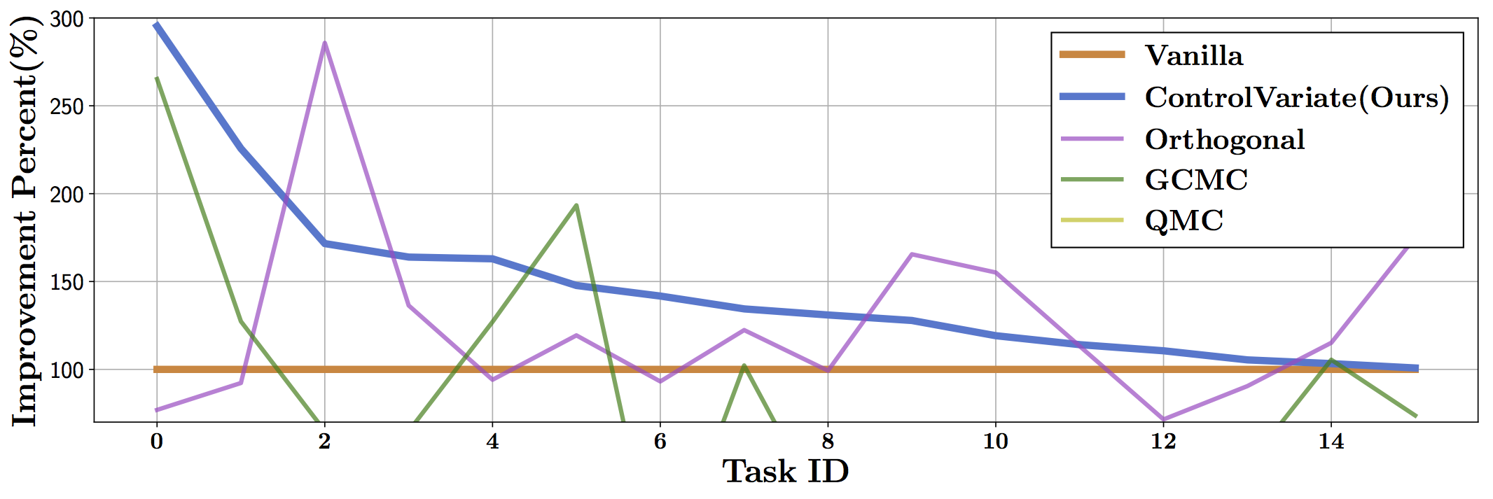
Figure 1: Percentile improvement over 16 benchmark tasks. The metric is calculated for each task as $(r_{\text{cv}}-r_{\text{random}})/(r_{\text{es}}-r_{\text{random}})$, where $r_{\text{cv}},r_{\text{es}},r_{\text{random}}$ are the final rewards for the rl tasks obtained with our control variate, vanilla es, and random policy methods respectively. We see that our proposal consistently improves over vanilla es for all tasks, and over all compared variance reduction methods for 10 out of 16 tasks. Section 4 provides additional details.

Related Work. Control variates are commonly used to reduce the variance of mc-based estimators (Ross, 2002). In black-box variational inference algorithms, carefully designed control variates can reduce the variance of mc gradient updates, leading to faster convergence (Paisley et al., 2012; Ranganath et al., 2014). In rl, pg methods apply state-dependent baseline functions as control variates (Mnih et al., 2016; Schulman et al., 2015b, 2017). While action-dependent control variates (Gu et al., 2017; Liu et al., 2017; Grathwohl et al., 2018; Wu et al., 2018) have been proposed to achieve further variance reduction, Tucker et al. (2018) recently showed that the reported performance gains may be due to subtle implementation details, rather than better baseline functions.

To leverage the mdp structure in developing a rl-specific control variate for es, we derive a gradient estimator for the es objective based on reparameterization (Kingma and Welling, 2014) and the pg estimator. The control variate is constructed as a difference between two alternative gradient estimators. Our approach is related to a control variate techniques developed for modeling discrete latent variables in variational inference (Tucker et al., 2017). The idea is to relax the discrete model into a differentiable one and construct the control variate as the difference between the score function gradient estimator and reparameterized gradient estimator of the relaxed model. We expand on this connection in Section 3.3.

2 Policy Optimization in Reinforcement Learning

Sequential decision making problems are often formulated as a mdp s. Consider an episode indexed by time. At any given time $t\geq 0$, an agent is in a state $s_{t}\in\mathcal{S}$. The agent then takes an action $a_{t}\in\mathcal{A}$, receives an instant reward $r_{t}=r(s_{t},a_{t})\in\mathbb{R}$, and transitions to the next state $s_{t+1}\sim p(\cdot\mid s_{t},a_{t})$, where $p$ is a distribution determining transitional probabilities. Define the policy $\pi:\mathcal{S}\mapsto\mathcal{P}(\mathcal{A})$ as a conditional distribution over actions $\mathcal{A}$ given a state $s\in\mathcal{S}$. Rl seeks to maximize the expected cumulative rewards over a given time horizon $T$,

$$J^{\gamma}(\pi) =\mathbb{E}_{\pi}\left[\sum_{t=0}^{T-1}r_{t}\gamma^{t}\right],$$ (1)

where $\gamma\in(0,1]$ is a discount factor and the expectation is with respect to randomized environment and outputs of the policy $\pi$.

Ideally, we would like to work with an infinite horizon and no discount factor. In practice, horizon $T$ is bounded by sample collection (Brockman et al., 2016) while directly optimizing the undiscounted objective $J^{1}(\pi)$ admits unusably high variance gradient estimators (Schulman et al., 2015b). As a result, modern rl algorithms tackle the problem through a discount factor $\gamma<1$, which reduces the variance of the gradient estimators but introduces bias (Schulman et al., 2015b, 2017; Mnih et al., 2016). At evaluation time, the algorithms are evaluated with finite horizons $T<\infty$ and undiscounted returns $\gamma=1$ (Schulman et al., 2015b, 2017; Mnih et al., 2016). We follow this setup here as well.

Consider parameterizing the policy as $\pi_{\theta}$ where $\theta\in\mathbb{R}^{d}$. The goal is to optimize Equation 1 with respect to policy parameters. A natural approach is to use exact gradient methods. Regrettably, this objective function does not admit an analytic gradient. Thus, we turn to stochastic gradient techniques (Robbins and Monro, 1951) and seek to construct approximations to the true gradient $g_{\theta}^{\gamma}=\nabla_{\theta}J^{\gamma}(\pi_{\theta})$.

2.1 Evolution Strategies for Policy Optimization

Evolution strategies (es) (Salimans et al., 2017) take a black-box optimization approach to maximizing Equation 1. To do so, the first step is to ensure that the objective function is differentiable with respect to the policy parameters. To this end, es begin by convolving the original objective $J^{\gamma}(\pi_{\theta})$ with a multivariate isotropic Gaussian distribution of mean $\theta$ and variance $\sigma^{2}$:

$$F^{\sigma,\gamma}(\theta) =\mathbb{E}_{\theta^{\prime}\sim\mathcal{N}(\theta,\sigma^{2}\mathbb{I})}\left[J^{\gamma}(\pi_{\theta^{\prime}})\right].$$ (2)

es maximize this smooth objective as a proxy to maximizing the original objective $J^{\gamma}(\pi_{\theta})$. The convolved objective $F$ enjoys the advantage of being differentiable with respect to the policy. In the limit $\sigma\rightarrow 0$, an optimal point of $F^{\sigma,\gamma}(\theta)$ is also optimal with respect to $J^{\gamma}(\pi_{\theta})$. The next step is to derive a gradient of Equation 2. Consider the score function gradient,

$$\nabla_{\theta}F^{\sigma,\gamma}(\theta) =\mathbb{E}_{\theta^{\prime}\sim\mathcal{N}(\theta,\sigma^{2}\mathbb{I})}\left[J^{\gamma}(\pi_{\theta^{\prime}})\frac{\theta^{\prime}-\theta}{\sigma^{2}}\right].$$ (3)

This gradient can be computed by sampling $\theta_{i}^{\prime}\sim\mathcal{N}(\theta,\sigma^{2}\mathbb{I})$ and computing unbiased estimates of each $J^{\gamma}(\pi_{\theta_{i}^{\prime}})$ using a single roll-out trajectory of $\pi_{\theta_{i}^{\prime}}$ in the environment. The resulting score function gradient estimator has the following form:

$$\hat{g}^{\textsc{es},\gamma}_{\theta}=\frac{1}{N}\sum_{i=1}^{N}J^{\gamma}(\pi_{\theta_{i}^{\prime}})\frac{\theta_{i}^{\prime}-\theta}{\sigma^{2}}.$$ (4)

This gradient estimator is biased with respect to the original objective. However, in practice this bias does not hinder optimization; on the contrary, the smoothed objective landscape is often more amenable to gradient-based optimization (Leordeanu and Hebert, 2008). We also make clear that though the es gradient is defined for any $\gamma\in(0,1]$, in practice parameters are updated with the gradient of the undiscounted objective $\hat{g}_{\theta}^{\text{ES},1}$ (Salimans et al., 2017; Mania et al., 2018; Choromanski et al., 2018).

2.2 Policy Gradient Methods for Policy Optimization

Policy gradient (pg) (Sutton et al., 2000) methods take a different approach. Instead of deriving the gradient through a parameter level perturbation as in es, the core idea of pg is to leverage the randomness in the policy itself. Using a standard procedure from stochastic computational graphs (Schulman et al., 2015a), we compute the gradient of Equation 1 as follows

$$\nabla_{\theta}J^{\gamma}(\pi_{\theta}) =\mathbb{E}_{\pi_{\theta}}\left[\sum_{t=0}^{T-1}\left(\sum_{t^{\prime}=t}^{T-1}r_{t^{\prime}}\right)\gamma^{t}\nabla_{\theta}\log\pi_{\theta}(a_{t}|s_{t})\right].$$ (5)

Unbiased estimators $\hat{g}^{\textsc{pg},\gamma}_{\theta}$ of this gradient can be computed using sampling as above for the es method. In practice, the sample estimate of Equation 5 often has large variance which destabilizes the updates. To alleviate this issue, one convenient choice is to set $\gamma<1$ so that the long term effects of actions are weighted down exponentially. This reduces the variance of the estimator, but introduces bias with respect to the original undiscounted objective $J^{1}(\pi_{\theta})$.

Es and pg are two alternative methods for deriving gradient estimators with respect to the policy parameters. On an intuitive level, these two methods complement each other for variance reduction: pg leverages the mdp structure and achieves lower variance when the policy is stochastic; es derives the gradient by injecting noise directly into the parameter space and is characterized by lower variance when the policy itself is near-deterministic. Our goal in this paper is to develop a single estimator that benefits from both approaches. We formalize this intuition in the next section.

3 Variance Reduction via Structured Control Variates

We seek a control variate for the es gradient estimator in Equation 4. Recall that this gradient is with respect to a smoothed objective: $F^{\sigma,\gamma}(\theta)$ with $\gamma\in(0,1]$.

3.1 Reparameterized Gradients of the Smoothed Objective

The es gradient estimator in Equation 4 leverages the derivative of the logarithm. We can also apply the reparameterization technique (Kingma and Welling, 2014) to the distribution $\theta^{\prime}\sim\mathcal{N}(\theta,\sigma^{2}\mathbb{I})$ to obtain:

$$\nabla_{\theta}F^{\sigma,\gamma}(\theta) =\nabla_{\theta}\mathbb{E}_{\theta^{\prime}\sim\mathcal{N}(\theta,\sigma^{2}\mathbb{I})}[J^{\gamma}(\pi_{\theta^{\prime}})]$$

$$=\nabla_{\theta}\mathbb{E}_{\epsilon\sim\mathcal{N}(0,\mathbb{I})}[J^{\gamma}(\pi_{\theta+\epsilon\cdot\sigma})]$$

$$=\mathbb{E}_{\epsilon\sim\mathcal{N}(0,\mathbb{I})}[\nabla_{\theta+\epsilon\cdot\sigma}J^{\gamma}(\pi_{\theta+\epsilon\cdot\sigma})],$$ (6)

where $\nabla_{\theta+\epsilon\cdot\sigma}J^{\gamma}(\pi_{\theta+\epsilon\cdot\sigma})$ can be computed by pg estimators for the discounted objective (5). To estimate (6), we sample $\epsilon_{i}\sim\mathcal{N}(0,\sigma^{2}\mathbb{I})$ and construct perturbed policies $\theta_{i}^{\prime}=\theta+\epsilon_{i}\cdot\sigma$. Then an unbiased estimate $\hat{g}^{\textsc{pg},\gamma}_{\theta+\epsilon_{i}\cdot\sigma}$ of the policy gradient $\nabla_{\theta+\epsilon_{i}\cdot\sigma}J^{\gamma}(\pi_{\theta+\epsilon_{i}\cdot\sigma})$ can be computed from a single rollout trajectory using $\pi_{\theta+\epsilon_{i}\cdot\sigma}$. Finally the reparameterized gradient is computed by averaging:

$$\hat{g}^{\textsc{re},\gamma}_{\theta}=\frac{1}{N}\sum_{i=1}^{N}\hat{g}^{\textsc{pg},\gamma}_{\theta+\epsilon_{i}\cdot\sigma}.$$ (7)

3.2 Evolution Strategies with Structured Control Variates

For the discounted objective $F^{\sigma,\gamma}(\theta)$ we have two alternative gradient estimators. One is constructed using the score function gradient estimator (see: Equation 4). The other uses the re-parameterization techqniue along with policy gradient estimators (see: Equation 7). Combining these two estimators with the vanilla es gradient for the undiscounted objective $\hat{g}^{\textsc{es},1}_{\theta}$, we get:

$$\hat{g}^{\textsc{cv}}_{\theta}=\hat{g}^{\textsc{es},1}_{\theta}+\eta\odot(\hat{g}^{\textsc{es},\gamma}_{\theta}-\hat{g}^{\textsc{re},\gamma}_{\theta}),$$ (8)

where $\eta$ is a vector of same dimension of $\theta$ and $\odot$ denotes an element-wise product. This scaling parameter $\eta$ controls the relative importance of the two terms in (8). As discussed below, we can adapt the discount factor $\gamma$ and the scaling parameter $\eta$ to minimize the variance over time.

Discount factor $\gamma$.

As in Choromanski et al. (2018), for a vector $g\in\mathbb{R}^{n}$, we define its variance as the sum of its component variances $\mathbb{V}[g]\coloneqq\sum_{i=1}^{n}\mathbb{V}[g_{i}]$. We then adapt the discount factor $\gamma\leftarrow\gamma-\alpha_{\gamma}\nabla_{\gamma}\mathbb{V}[\hat{g}_{\theta}^{\textsc{cv}}]$ for some learning rate $\alpha_{\gamma}>0$. Since $\mathbb{E}[\hat{g}_{\theta}^{\textsc{cv}}]$ does not depend on $\gamma$, we have equivalently $\nabla_{\gamma}\mathbb{V}[\hat{g}_{\theta}^{\textsc{cv}}]=\nabla_{\gamma}\mathbb{E}[(\hat{g}_{\theta}^{\textsc{cv}})^{2}]$. The gradient $\nabla_{\gamma}\mathbb{E}[(\hat{g}_{\theta}^{\textsc{cv}})^{2}]$ can be itself estimated using backpropagation on mini-batches but this tends to be unstable because each term in (5) involves $\gamma^{t}$. Alternatively, we build a more robust estimator of $\nabla_{\gamma}\mathbb{E}[(\hat{g}_{\theta}^{\textsc{cv}})^{2}]$ using es: in particular, sample $\epsilon_{i}\sim\mathcal{N}(0,1)$ and let $v_{i}$ be the evaluation of $\mathbb{E}[(\hat{g}_{\theta}^{\textsc{cv}})^{2}]$ under $\gamma+\sigma_{\gamma}\epsilon_{i}$ for some $\sigma_{\gamma}>0$. The gradient estimator for $\gamma$ is $\hat{g}_{\gamma}=\frac{1}{N}\sum_{i=1}^{N}v_{i}\frac{\epsilon_{i}}{\sigma_{\gamma}}$.

Though the full estimator (8) is defined for all discount factors $\gamma\in(0,1]$, in general we find it better to set $\gamma<1$ to stablize the pg components of the control variate.

Coefficient $\eta$.

Since $\eta$ is a vector with the same dimensionality as $\theta$, we can update each component of $\eta$ to reduce the variance of each component of $\hat{g}_{\theta}^{\textsc{cv}}$. Begin by computing, $\nabla_{\eta}\mathbb{V}[\hat{g}_{\theta}^{\textsc{cv}}]$ as follows:

$$\nabla_{\eta}\mathbb{V}\bigg{[}\hat{g}_{\theta}^{\textsc{cv}}\bigg{]} =2\eta\odot\mathbb{E}\bigg{[}\big{(}\hat{g}^{\textsc{es},\gamma}_{\theta}-\hat{g}^{\textsc{re},\gamma}_{\theta}\big{)}^{2}\bigg{]}+$$

$$2\mathbb{E}\bigg{[}\big{(}\hat{g}^{\textsc{es},\gamma}_{\theta}-\hat{g}^{\textsc{re},\gamma}_{\theta}\big{)}\odot\hat{g}_{\theta}^{\textsc{es},1}\bigg{]}.$$ (9)

Then, estimate this gradient using mc sampling. Finally, adapt $\eta$ by running online gradient descent: $\eta\leftarrow\eta-\alpha_{\eta}\nabla_{\eta}\mathbb{V}[\hat{g}_{\theta}^{\textsc{cv}}]$ with some $\alpha_{\eta}>0$.

Practical considerations.

Certain practical techniques can be applied to stabilize the es optimization procedure. For example, Salimans et al. (2017) apply a centered rank transformation to the estimated returns $J^{\gamma}(\pi_{\theta_{i}^{\prime}})$ to compute the estimator of the gradient in Equation 4. This transformation is compatible with our proposal. The construction becomes $\hat{g}_{\theta}^{\textsc{cv}}=\hat{g}_{\theta}+\eta(\hat{g}^{\textsc{es},\gamma}_{\theta}-\hat{g}^{\textsc{re},\gamma}_{\theta})$ where $\hat{g}_{\theta}$ can be computed through the rank transformation.

Stochastic policies.

While many prior works (Salimans et al., 2017; Mania et al., 2018; Choromanski et al., 2018; Rowland et al., 2018) focus on deterministic policies for continuous action spaces, our method targets stochastic policies, as required by the pg computation. Estimating pg for a deterministic policy requires training critic functions and is in general biased (Silver et al., 2014). We leave the investigation of deterministic policies to future work.

3.3 Relationship to REBAR

REBAR (Tucker et al., 2017) considers variance reduction of gradient estimators for probabilistic models with discrete latent variables. The discrete latent variable model has a relaxed model version, where the discrete sampling procedure is replaced by a differentiable function with reparameterized noise. This relaxed model usually has a temperature parameter $\tau$ such that when $\tau\rightarrow 0$ the relaxed model converges to the original discrete model. To optimize the discrete model, the baseline approach is to use score function gradient estimator, which is unbiased but has high variance. Alternatively, one could use the reparameterized gradient through the relaxed model, which has lower variance, but the gradient is biased for finite $\tau>0$ (Jang et al., 2017; Maddison et al., 2017). The bias and variance of the gradient through the relaxed model is controlled by $\tau$. REBAR proposes to use the difference between the score function gradient and reparameterized gradient of the relaxed model as a control variate. Their difference has expectation zero and should be highly correlated with the reinforced gradient of the original discrete model, leading to potentially large variance reduction.

A similar connection can be found in es for rl context. We can interpret the non-discounted objective, namely $F^{\sigma,\gamma}(\pi_{\theta})$ with $\gamma=1$, as the original model which gradient we seek to estimate. When $\gamma<1$, we have the relaxed model which gradient becomes biased but has lower variance (with respect to the non-discounted objective). Similar to REBAR, our proposal is to construct the score function gradient (es estimator) $\hat{g}_{\theta}^{\textsc{es},\gamma}$ and reparameterized gradient (pg estimator) $\hat{g}_{\theta}^{\textsc{re},\gamma}$ of the general discounted objective $\gamma<1$ (relaxed model), such that their difference $\hat{g}_{\theta}^{\textsc{es},\gamma}-\hat{g}_{\theta}^{\textsc{re},\gamma}$ serves as a control variate. The variance reduction from REBAR applies here, $\hat{g}_{\theta}^{\textsc{es},\gamma}-\hat{g}_{\theta}^{\textsc{re},\gamma}$ should be highly correlated with $\hat{g}_{\theta}^{\textsc{es},1}$, which leads to effective variance reduction.

3.4 How much variance reduction is possible?

How does the variance reduction provided by control variate compare to that of general purpose methods, such as orthogonalization (Choromanski et al., 2018)? In this section, we build on a simple example to illustrate the different variance reduction properties of these approaches. Recall that we define the variance of a vector $g\in\mathbb{R}^{d}$ as the sum of the variance of its components $\mathbb{V}[g]=\sum_{i=1}^{d}\mathbb{V}[g_{i}]$ following notation from prior literature (Choromanski et al., 2018; Rowland et al., 2018).

Consider a one-step mdp problem where the agent takes only one action $a$ and receives a reward $r(a)=\alpha^{T}a$ for some $\alpha\in\mathbb{R}^{d}$. We choose the reward function to be linear in $a$, as a local approximation to a potentially nonlinear reward function landscape. Let the policy be a Gaussian with mean $\mu$ and diagonal covariance matrix $\Sigma=\sigma_{2}^{2}\mathbb{I}$ with fixed $\sigma_{2}$. Here the policy parameter contains only the mean $\theta=\mu$. The rl objective is $J(\pi_{\mu})=\mathbb{E}_{a\sim\mathcal{N}(\mu,\Sigma)}[r(a)]$. To compute the gradient, es smoothes the objective with the Gaussin $\mathcal{N}(\mu,\sigma_{1}^{2}\mathbb{I})$ for a fixed $\sigma_{1}$. While vanilla es generates i.i.d. perturbations $\epsilon_{i}$, orthogonal es couples the perturbations such that ${\epsilon_{i}^{\prime}}^{T}\epsilon_{j}^{\prime}=0,i\neq j$.

Denote $d$ as the dimensionality of the parameter space $\mu\in\mathbb{R}^{d}$ and let $\rho=\nicefrac{{\sigma_{2}}}{{\sigma_{1}}}$. Let $\hat{J}(\pi_{\mu 1})$ be a one-sample noisy estimate of $J(\pi_{\mu})$. Recall that es gradient takes the form $\hat{g}_{\mu}^{\textsc{es}}=\nicefrac{{1}}{{N}}\sum_{i=1}^{N}\hat{J}(\pi_{\mu+\sigma_{1}\epsilon_{i}})\>\nicefrac{{\epsilon_{i}}}{{\sigma_{1}}}$ (eq. 4). The orthogonal es gradient takes the same form, but with orthogonal perturbations $\hat{g}_{\mu}^{\text{ort}}=\nicefrac{{1}}{{N}}\sum_{i=1}^{N}\hat{J}(\pi_{\mu+\sigma_{1}\epsilon_{i}^{\prime}})\>\nicefrac{{\epsilon_{i}^{\prime}}}{{\sigma_{1}}}$. Finally, the es with control variate produces an estimator of the form (8). We are now ready to provide the following theoretical result.

Theorem 1.

In the one-step mdp described above, the ratio of the variance of the orthogonal es to the variance of the vanilla es, and the corresponding ratio for the control variate es satisfy respectively:

$$\ \ \ \ \ \ \ \ \ \frac{\mathbb{V}[\hat{g}_{\mu}^{\text{ort}}]}{\mathbb{V}[\hat{g}_{\mu}^{\textsc{es}}]} =1-\frac{N-1}{(1+\rho^{2})d+1},$$

$$\ \ \frac{\mathbb{V}[\hat{g}_{\mu}^{\textsc{cv}}]}{\mathbb{V}[\hat{g}_{\mu}^{\textsc{es}}]} \leq 1-\frac{\rho^{2}[d((1+\rho^{2})-4]}{[(1+\rho^{2})d+1](1+\rho^{2})}.$$

As a result, there exists a threshold $\rho_{0}$ such that when $\rho\geq\rho_{0}$, we always have $\mathbb{V}[\hat{g}_{\mu}^{\textsc{cv}}]\leq\mathbb{V}[\hat{g}_{\mu}^{\text{ort}}]$. (See: Appendix for details). Importantly, when $d$ is large enough, we have $\rho_{0}\rightarrow\sqrt{\nicefrac{{N}}{{d}}}$.

Some implications of the above theorem: (1) For orthogonal es, the variance reduction depends explicitly on the sample size $N$. In cases where $N$ is small, the variance gain over vanilla es is not significant. On the other hand, $\mathbb{V}[\hat{g}_{\mu}^{\textsc{cv}}]$ depends implicitly on $N$ because in practice $\eta^{\ast}$ is approximated via gradient decent and large sample size $N$ leads to more stable updates; (2) The threshold $\rho_{0}$ is useful in practice. In high-dimensional applications where sample efficiency is important, we have large $d$ and small $N$. This implies that for a large range of the ratio $\rho=\frac{\sigma_{2}}{\sigma_{1}}\geq\rho_{0}$, we could expect to achieve more variance reduction than orthogonal es. (3) The above derivation is based on the simplification of the general multi-step mdp problem. The practical performance of the control variate can also be influenced by how well $\eta^{\ast}$ is estimated. Nevertheless, we expect this example to provide some guideline as to how the variance reduction property of es with control variate depends on $\rho$ and $N$, in contrast to orthogonal es; (4) The theoretical guarantee for variance reduction of orthogonal es (Choromanski et al., 2018) relies on the assumption that $\hat{J}(\pi_{\theta^{\prime}})$ can be simulated without noise , which does not hold in practice. In fact, in rl the noise of the reward estimate heavily depends on the policy $\pi_{\theta^{\prime}}$ (intuitively the more random the policy is, the more noise there is in the estimate). On the other hand, es with control variate depends less on such assumptions but rather relies on finding the proper scalar $\eta$ using gradient descent. We will see in the experiments that this latter approach reliably improves upon the es baseline.

4 Experiments

In the experiments, we aim to address the following questions: (1): Does the control variate improve downstream training through variance reduction? (2): How does it compare with other recent variance reduction techniques for es?

To address these questions, we compare our control variate to general purpose variance reduction techniques on a wide range of high-dimensional rl tasks with continuous action space.

Antithetic sampling:

See Salimans et al. (2017). Let $\epsilon_{i},1\leq i\leq N$ be the set of perturbation directions. Antithetic sampling perturbs the policy parameter with a set of antithetic pairs $(\epsilon_{i},\epsilon_{i}^{\prime}),1\leq i\leq N$ where $\epsilon_{i}^{\prime}=-\epsilon_{i}$.

Orthogonal directions (ORTHO):

See Choromanski et al. (2018). The set of perturbations $\epsilon_{i},1\leq i\leq N$ applied to the policy parameter are generated such that they have the same marginal Gaussian distributions but are orthogonal to each other $\epsilon_{i}^{T}\epsilon_{j}=0,i\neq j$.

Geometrically coupled MC sampling (GCMC):

See Rowland et al. (2018). For each antithetic pair $(\epsilon_{i},\epsilon_{i}^{\prime})$, GCMC couples their length such that $F_{R}(\|\epsilon_{i}\|)+F_{R}(\|\epsilon_{i}^{\prime}\|)=1$ where $F_{R}$ is the CDF of the norm of a standard Gaussian with the same dimension as $\epsilon_{i}$.

Quasi Monte-Carlo (QMC):

See Choromanski et al. (2018); Rowland et al. (2018). QMC first generates a low-discrepancy Halton sequence $\{r_{i}\}_{i=1}^{N}$ in $[0,1]^{d}$ with $N$ elements where $d$ is the dimension of parameter $\theta$. Then apply the inverse CDF $F_{g}^{-1}$ of a standard univariate Gaussian elementwise to the sequence $\epsilon_{i}=F_{g}^{-1}(r_{i})$ to generate perturbation vectors.

We find that our rl-specific control variate achieves outperforms these general purpose variance reduction techniques. In addition to the above baseline comparison, we also compare CV with more advanced policy gradient algorithms such as TRPO / PPO (Schulman et al., 2015b, 2017), as well as deterministic policy $+$ es baseline (Mania et al., 2018).

Implementation details. Since antithetic sampling is the most commonly applied variance reduction method, we combine it with the control variate, ORTHO, GCMC and QMC. The policy $\pi_{\theta}$ is parameterized as a neural network with 2 hidden layers each with 32 units and relu activation function. The output is a vector $\mu_{\theta}\in\mathbb{R}^{K}$ used as a Gaussian mean, with a separately parameterized diagonal vector $\sigma_{0}\in\mathbb{R}^{K}$ independent of state. The action is sampled the Gaussian $a\sim\mathcal{N}(\mu_{\theta}(s),\text{diag}(\sigma^{2}))$. The backpropagation pipeline is implemented with Chainer (Tokui et al., 2015). The learning rate is $\alpha=0.01$ with Adam optimizer (Kingma and Ba, 2014), the perturbation standard deviation $\sigma=0.02$. At each iteration we have $N=5$ distinct perturbations $\epsilon_{i}$ ($2N$ samples in total due to antithetc sampling). For the control variate (8), the discount factor is initialized to be $\gamma=0.99$ and updated with es, we introduce the details in the Appendix. The control variate scaling factor $\eta$ is updated with learning rate selected from $\alpha_{\eta}\in\{10^{-3},10^{-4},10^{-5}\}$. As commonly practiced in prior works (Salimans et al., 2017; Mania et al., 2018; Choromanski et al., 2018), in order to make the gradient updates less sensitive to the reward scale, returns are normalized before used for computing the gradients. We adopt this technique and discuss the details in the Appendix. Importantly, we do not normalize the observations (as explained in (Mania et al., 2018)) to avoid additional biasing of the gradients.

Benchmark tasks and baselines. To evaluate how variance reduction impacts downstream policy optimization, we train neural network policies over a wide range of high-dimensional continuous control tasks, taken from OpenAI gym (Brockman et al., 2016), Roboschool (Schulman et al., 2017) and DeepMind Control Suites (Tassa et al., 2018). We introduce their details below. We also include a LQR task suggested in (Mania et al., 2018) to test the stability of the gradient update for long horizons ($T=2000$). Details of the tasks are in the Appendix. The policies are trained with five variance reduction settings: Vanilla es baseline; es with orthogonalization (ORTHO); es with GCMC (GCMC); es with Quasi-mc (QMC); and finally our proposed es with control variate (CV).

Results.

In each subplot of Figure 2, we present the learning curves of each variance reduction technique, with average performance over 5 random seeds and the shaded areas indicate standard deviations.

We make several observations regarding each variance reduction technique: (1) Though ORTHO and GCMC significantly improve the learning progress over the baseline es under certain settings (e.g. ORTHO in Swimmer and GCMC), their improvement is not very consistent. In certain cases, adding such techniques even makes the performance worse than the baseline es. We speculate that this is because the variance reduction conditions required by these methods are not satisfied, e.g. the assumption of noiseless estimate of returns. Overall, ORTHO is more stable than GCMC and QMC; (2) QMC performs poorly on most tasks. We note that similar results have been reported in (Rowland et al., 2018) where they train a navigation policy using QMC and show that the agent does not learn at all. We speculate that this is because the variance reduction achieved by QMC is not worth the bias in the rl contexts; (3) No variance reduction technique performs uniformly best across all tasks. However, CV performs the most consistently and achieves stable gains over the vanilla es baseline, while other methods can underperform the vanilla es baseline.

To make clear the comparison of final performance, we record the final performance (mean $\pm$ std) of all methods in Table 1. Best results across each task are highlighted in bold font. For a fair presentation of the results, in cases where multiple methods achieve statistically similar performance, we highlight all such methods. CV consistently achieves the top results across all reported tasks.

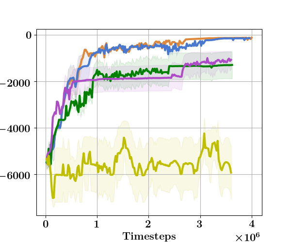
(a) LQR

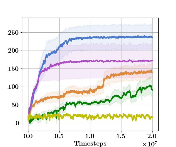
(b) Swimmer

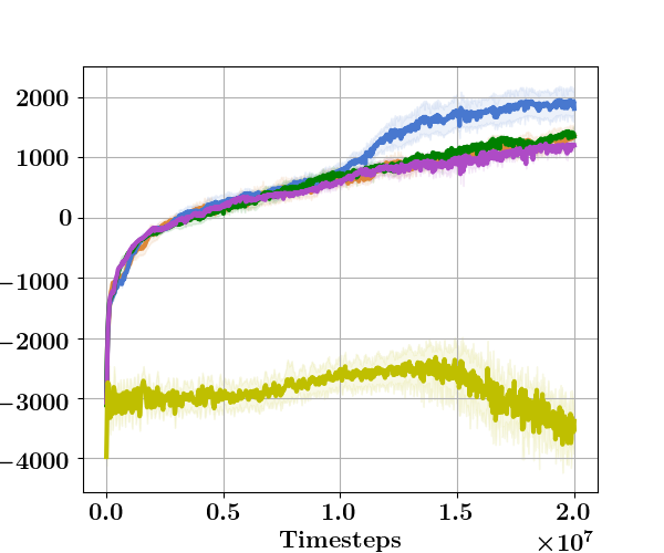
(c) HalfCheetah

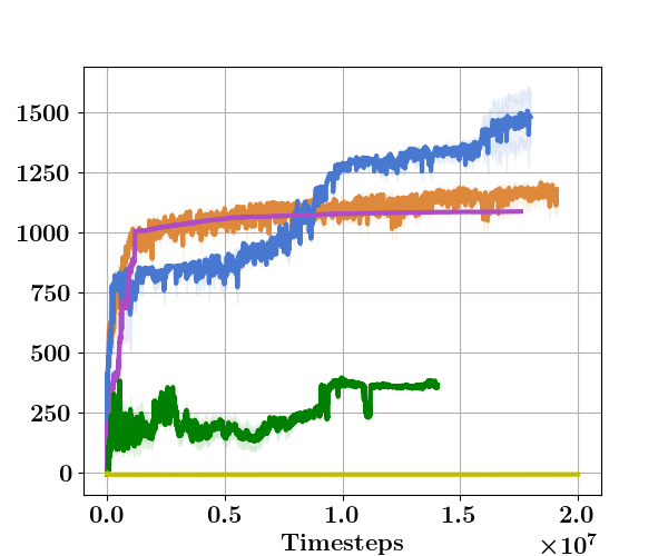
(d) Walker

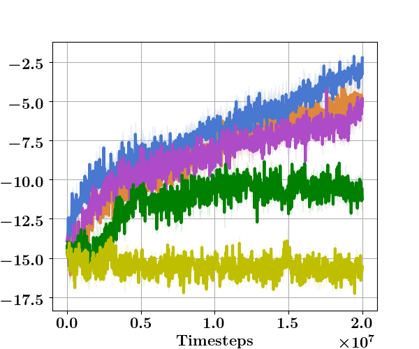
(e) RoboschoolPong

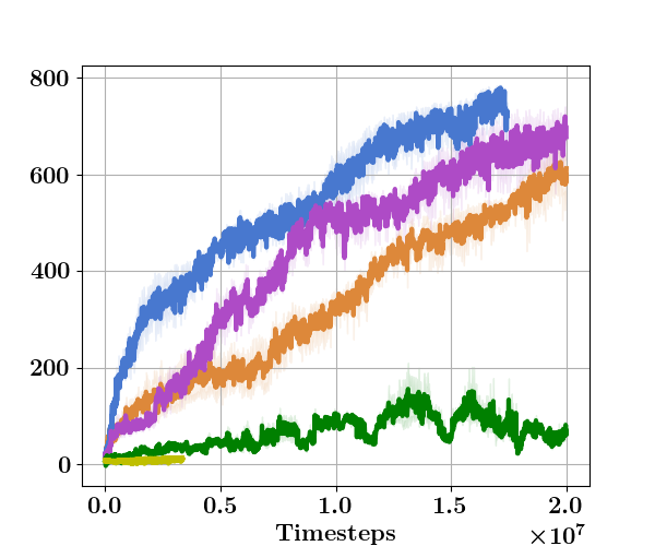
(f) RoboschoolCheetah

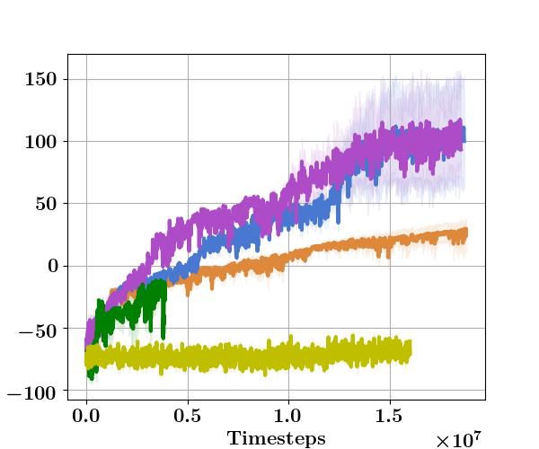
(g) BipedalWalker

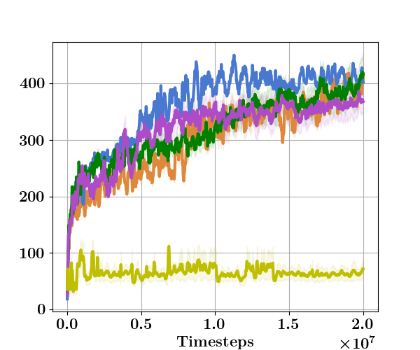
(h) Swingup (DM)

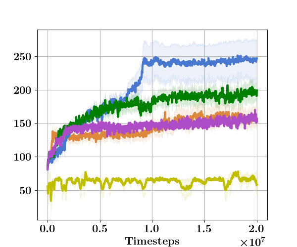
(i) TwoPoles (DM)

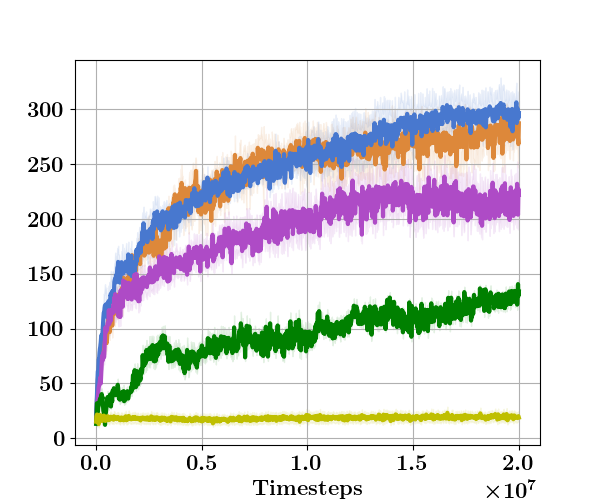
(j) CheetahRun (DM)

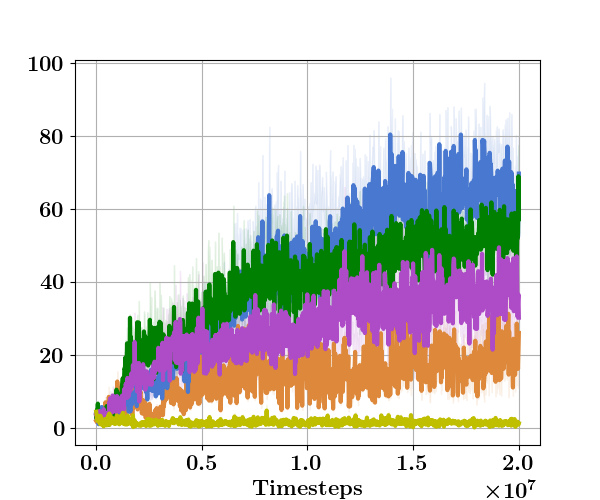
(k) HopperStand (DM)

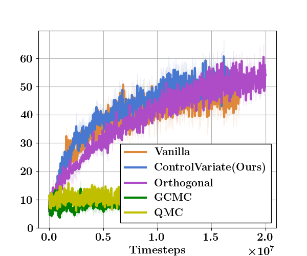
(l) AntEscape(DM)

Figure 2: Training performance on Continuous Control Benchmarks: Swimmer, HalfCheetah, CartPole $+$ $\{\text{Swingup},\text{TwoPoles},\text{Balance}\}$, Pendulum Swingup, Cheetah Run and Hopper. Tasks with DM stickers are from the DeepMind Control Suites. We compare five alternatives: baseline ES (orange), CV (blue, ours), ORTHO (marron), GCMC (green) and QMC (yellow). Each task is trained for $2\cdot 10^{7}$ time steps (LQR is trained for $4\cdot 10^{6}$ steps) and the training curves show the mean $\pm$ std cumulative rewards across 5 random seeds.

Table 1: Final performance on benchmark tasks. The policy is trained for a fixed number of steps on each task. The result is $\text{mean}\pm\text{std}$ across 5 random seeds. The best results are highlighted in bold font. We highlight multiple methods if their results cannot be separated ($\text{mean}\pm\text{std}$ overlap). CV (ours) achieves consistent gains over the baseline and other variance reduction methods. We also include a pg baseline.

Tasks	Vanilla ES	Orthogonal	GCMC	QMC	CV (Ours)	PG
LQR	$-176\pm 12$	$-1337\pm 573$	$-1246\pm 502$	$-5634\pm 1059$	$\mathbf{-143\pm 4}$	$-7243\pm 275$
Swimmer	$141\pm 20$	$171\pm 47$	$94\pm 19$	$16\pm 2$	$\mathbf{237\pm 33}$	$-132\pm 5$
HalfCheetah	$1339\pm 178$	$1185\pm 76$	$1375\pm 58$	$-3466\pm 338$	$\mathbf{1897\pm 232}$	$-180\pm 4$
Walker	$1155\pm 34$	$1087\pm 1$	$360\pm 4$	$6\pm 0$	$\mathbf{1476\pm 112}$	$282\pm 25$
Pong(R)	$-5.0\pm 0.8$	$-5.5\pm 0.3$	$-10.6\pm 0.4$	$-15.6\pm 0.3$	$\mathbf{-3.0\pm 0.3}$	$-17\pm 0.2$
HalfCheetah(R)	$\mathbf{595\pm 42}$	$\mathbf{685\pm 34}$	$68\pm 8$	$11\pm 2$	$\mathbf{709\pm 16}$	$12\pm 0$
BipedalWalker	$25\pm 9$	$\mathbf{107\pm 31}$	$-19\pm 5$	$-70\pm 3$	$\mathbf{105\pm 40}$	$-82\pm 12$
Cheetah(DM)	$281\pm 15$	$217\pm 15$	$129\pm 4$	$18\pm 5$	$\mathbf{296\pm 15}$	$25\pm 6$
Pendulum(DM)	$20\pm 3$	$\mathbf{54\pm 17}$	$25\pm 8$	$11\pm 2$	$\mathbf{43\pm 1}$	$3\pm 1$
TwoPoles(DM)	$159\pm 13$	$158\pm 2$	$196\pm 12$	$62\pm 12$	$\mathbf{245\pm 29}$	$14\pm 1$
Swingup(DM)	$\mathbf{394\pm 15}$	$\mathbf{369\pm 22}$	$\mathbf{414\pm 31}$	$67\pm 14$	$\mathbf{406\pm 26}$	$55\pm 10$
Balance(DM)	$692\pm 57$	$771\pm 41$	$\mathbf{995\pm 1}$	$223\pm 32$	$\mathbf{847\pm 71}$	$401\pm 12$
HopperHop(DM)	$\mathbf{5.7\pm 2.1}$	$\mathbf{6.8\pm 0.7}$	$0.3\pm 0.1$	$0.0\pm 0.0$	$\mathbf{6.5\pm 1.5}$	$0.1\pm 0.0$
Stand(DM)	$21\pm 5$	$36\pm 10$	$\mathbf{54\pm 4}$	$1.0\pm 0.2$	$\mathbf{60\pm 11}$	$0.5\pm 0.1$
AntWalk(DM)	$\mathbf{200\pm 19}$	$\mathbf{234\pm 10}$	$82\pm 11$	$133\pm 9$	$\mathbf{239\pm 10}$	$100\pm 11$
AntEscape(DM)	$\mathbf{47\pm 3}$	$\mathbf{52\pm 3}$	$8\pm 2$	$10\pm 1$	$\mathbf{51\pm 2}$	$6\pm 1$

Table 2: Final performance on benchmark tasks. The setup is the same as in Table 2. CV (ours) achieves consistent gains over deterministic policy $+$ es as well as more advanced baselines such as TRPO and PPO. We also include a pg baseline for easy comparison. In the following, ’Det’ denotes the deterministic policies.

Tasks	PPO	TRPO	Det	CV (Ours)	PG
Swimmer	$11\pm 7$	$11\pm 7$	$191\pm 100$	$\mathbf{237\pm 33}$	$-132\pm 5$
HalfCheetah	$-175\pm 20$	$-174\pm 16$	$1645\pm 1298$	$\mathbf{1897\pm 232}$	$-180\pm 4$
Walker	$657\pm 291$	$657\pm 292$	$1588\pm 744$	$\mathbf{1476\pm 112}$	$282\pm 25$
Pong(R)	$-17.1\pm 0.4$	$-15.0\pm 2.6$	$-10.4\pm 5.4$	$\mathbf{-3.0\pm 0.3}$	$-17\pm 0.2$
HalfCheetah(R)	$14\pm 2$	$13\pm 3$	$502\pm 199$	$\mathbf{709\pm 16}$	$12\pm 0$
BipedalWalker	$-66\pm 39$	$-66\pm 38$	$1\pm 2$	$\mathbf{105\pm 40}$	$-82\pm 12$
Pendulum(DM)	$0.6\pm 0.5$	$7.5\pm 4.8$	$40\pm 16$	$\mathbf{43\pm 1}$	$3\pm 1$
Balance(DM)	$264\pm 46$	$515\pm 42$	$692\pm 250$	$\mathbf{847\pm 71}$	$401\pm 12$
HopperHop(DM)	$0.2\pm 0.2$	$0.0\pm 0.0$	$4.6\pm 6.2$	$\mathbf{6.5\pm 1.5}$	$0.1\pm 0.0$
AntWalk(DM)	$96\pm 36$	$180\pm 41$	$192\pm 20$	$\mathbf{239\pm 10}$	$100\pm 11$

Comparison with Policy Gradients.

A natural question is what happens when we update the policy just based on the pg estimator? We show the complete comparison in Table 1, where we find pure pg to be mostly outperformed by the other es baselines. We speculate that this is because the vanilla pg are themselves quite unstable, as commonly observed in prior works on pg which aim to alleviate the instability by introducing bias in exchange for smaller variance (Schulman et al., 2015b; Mnih et al., 2016; Schulman et al., 2017). We provide a detailed review in the Appendix. This comparison also implies that a careful control variate scheme can extract the benefit of pg estimators for variance reduction in es, instead of completely relying on pg.

To assess the impact of our method, we also compare with trust-region based on-policy pg algorithms: TRPO (Schulman et al., 2015b) and PPO (Schulman et al., 2017). Instead of a batched implementation as in the original paper, we adopt a fully on-line pg updates to align with the way es baselines are implemented. We list detailed hyper-parameters and implementations in the Appendix C. Due to space limit, the results of selected tasks are presented in table 2 and we leave a more comprehensive set of results in the Appendix.

We see that the trust-region variants lead to generally more stable performance than the vanilla pg. Nevertheless, the performance of these algorithms do not match those of the es baselines. There are several enhancements one can make to improve these pg baselines, all generally relying on biasing the gradients in exchange for smaller variance, e.g. normalizing the observations and considering a biased objective (Dhariwal et al., 2017). While here we consider only the ’unbiased’ pg methods, we discuss these methods in the Appendix.

Comparison with ES baselines.

As mentioned in Section 3, the CV is applicable only in cases where policies are stochastic. However, prior works consider mainly deterministic policy for continuous control (Mania et al., 2018; Choromanski et al., 2018). To assess the effects of policy choices, we adopt the same es baseline pipeline but with deterministic policies. The results of deterministic policies are reported in Table 2. We make several observations: (1) Deterministic policies generally perform better than stochastic policies when using es baselines. We speculate this is because the additional noise introduced by the stochastic policy is not worth the additional variance in the gradient estimation. Nevertheless, CV can leverage the variance reduction effects thanks to the stochastic policy, and maintain generally the best performance across tasks. Such comparison illustrates that it is beneficial to combine stochastic policies with es methods as long as there is proper variance reduction.

Practical Scalability.

In practical applications, the scalability of algorithms over large computational architecture is critical. Since CV blends ideas from es with pg, we require both distributed sample collection (Salimans et al., 2017; Mania et al., 2018) and distributed gradient computation (Dhariwal et al., 2017). Since both components can be optimally implemented over large architectures, we expect CV to properly scale. A more detailed discussion is in the Appendix.

5 Conclusion

We constructed a control variate for es that take advantage of the mdp structure of rl problems to improve on state-of-the-art variance reduction methods for es algorithms. Training algorithms using our control variate outperform those applying general-purpose mc methods for variance reduction. We provided theoretical insight into the effectiveness of our algorithm as well as exhaustive comparison of its performance with other methods on the set of over 16 rl benchmark tasks. In principle, this control variate can be combined with other variance reduction techniques; this may lead to further performance gains.

We leave as future work to study how similar structured control variates can be applied to improve the performance of state-of-the-art pg algorithms, in particular, cases where gradients have already been deliberately biased to achieve better performance such as in (Dhariwal et al., 2017).

Appendix A How Much Variance Reduction is Possible?

Recall in the main paper we consider a one-step MDP with action $a\in\mathbb{R}^{d}$. The reward function is $\alpha^{T}a$ for some $\alpha\in\mathbb{R}^{d}$. Consider a Gaussian policy with mean parameter $\mu$ and fixed covariance matrix $\Sigma=\sigma_{2}^{2}\mathbb{I}$. The action is sampled as $a\sim\mathcal{N}(\mu,\Sigma)$. ES convolves the reward objective with a Gaussian with covariance matrix $\sigma_{1}^{2}\mathbb{I}$. Let $\epsilon_{1}^{(i)},\epsilon_{2}^{(i)}\sim\mathcal{N}(0,\mathbb{I}),1\leq i\leq N$ be $N$ independent reparameterized noise, we can derive the vanilla ES estimator

$$\hat{g}_{\mu}^{\textsc{es}}=\frac{1}{N}\sum_{i=1}^{N}\hat{g}_{\mu,i}^{\textsc{es}}=\frac{1}{N}\sum_{i=1}^{N}\alpha^{T}(\mu+\sigma_{1}\epsilon_{1}^{(i)}+\sigma_{2}\epsilon_{2}^{(i)})\frac{\epsilon_{2}^{(i)}}{\sigma_{2}}$$

The orthogonal estimator is constructed by $N$ perturbations $\epsilon_{2,\text{ort}}^{(i)}$ such that $\langle\epsilon_{2,\text{ort}}^{(i)},\epsilon_{2,\text{ort}}^{(j)}\rangle=0$ for $i\neq j$, and each $\epsilon_{2}^{(i)}$ is still marginally $d$-dimensional Gaussian. The orthogonal estimator is

$$\hat{g}_{\mu}^{\text{ort}}=\frac{1}{N}\sum_{i=1}^{N}\hat{g}_{\mu,i}^{\text{ort}}=\frac{1}{N}\sum_{i=1}^{N}\alpha^{T}(\mu+\sigma_{1}\epsilon_{1}^{(i)}+\sigma_{2}\epsilon_{2,\text{ort}}^{(i)})\frac{\epsilon_{2,\text{ort}}^{(i)}}{\sigma_{2}}$$

Finally, we consider the ES gradient estimator with control variate. In particular, we have the reparameterized gradient as

$$\hat{g}_{\mu}^{\textsc{re}}=\frac{1}{N}\sum_{i=1}^{N}\hat{g}_{\mu,i}^{\textsc{re}}=\frac{1}{N}\sum_{i=1}^{N}\alpha^{T}(\mu+\sigma_{1}\epsilon_{1}^{(i)}+\sigma_{2}\epsilon_{2}^{(i)})\frac{\epsilon_{1}^{(i)}}{\sigma_{1}}$$

The general gradient estimator with control variate is

$$\hat{g}_{\mu}^{\textsc{cv}}=\hat{g}_{\mu}^{\textsc{es}}+\eta\odot(\hat{g}_{\mu}^{\textsc{re}}-\hat{g}_{\mu}^{\textsc{es}})$$

where $\eta\in\mathbb{R}^{d}$. Since $\eta$ can be indepdently chosen across dimensions, the maximal variance reduction is achieved by setting $\eta_{i}=-\frac{\text{cov}(X_{i},Y_{i})}{\mathbb{V}[Y_{i}]}$ where here $X=\hat{g}_{\mu}^{\textsc{es}},Y=\hat{g}_{\mu}^{\textsc{re}}-\hat{g}_{\mu}^{\textsc{es}}$.

Recall that for a vector $g$ of dimension $d$, its variance is defined as the sum of the variance of its components $\mathbb{V}[g]=\sum_{i=1}^{d}\mathbb{V}[g_{i}]$. For simplicity, let $\rho=\frac{\sigma_{2}}{\sigma_{1}}$. We derive the variance for each estimator below.

Vanilla ES.

For the vanilla ES gradient estimator, the variance is

$$\mathbb{V}[\hat{g}_{\mu}^{\textsc{es}}]=\frac{d+1}{N}\|\alpha\|_{2}^{2}$$

Orthogonal ES.

For the orthogonal ES gradient estimator, the variance is

$$\mathbb{V}[\hat{g}_{\mu}^{\text{ort}}]=\frac{(1+\rho^{2})d+2-N}{N}\|\alpha\|_{2}^{2}$$

ES with Control Variate.

For the ES gradient estimator with control variate, recall the above notation $X=\hat{g}_{\mu}^{\textsc{es}},Y=\hat{g}_{\mu}^{\textsc{re}}-\hat{g}_{\mu}^{\textsc{es}}$. We first compute $\rho(X_{p},Y_{p})^{2}=\frac{\text{cov}^{2}(X_{p},Y_{p})}{\mathbb{V}[X_{p}]\mathbb{V}[Y_{p}]}$ for each component $p$. Let $X_{p,i},Y_{p,i}$ be the $p$th component of $\hat{g}_{\mu,i}^{\textsc{es}}$ and $\hat{g}_{\mu,i}^{\textsc{re}}-\hat{g}_{\mu,i}^{\textsc{es}}$ respectively. We will detail how to compute $\text{cov}(X_{p},Y_{p}),\mathbb{V}[V_{p}]$ in the next section. With these components in hand, we have the final variance upper bound

$$\mathbb{V}[\hat{g}_{\mu}^{\textsc{cv}}] \leq\mathbb{V}[\hat{g}_{\mu}^{\textsc{es}}]\{1-\frac{(1+\rho^{2})[d((1+\rho^{2})-4]}{[(1+\rho^{2})d+1](2+\rho^{2}+\frac{1}{\rho^{2}})}\}.$$

Appendix B Derivation Details

Recall that for a vector $g$ of dimensioon $d$, we define its variance as $\mathbb{V}[g]=\sum_{i=1}^{d}\mathbb{V}[g_{i}]$ For simplicity, recall that $\rho=\frac{\sigma_{2}}{\sigma_{1}}$.

B.1 Variance of Orthogonal ES

We derive the variance of orthogonal ES based on the formula in the Appendix of (Choromanski et al., 2018). In particular, we can easily compute the $i$ sample estimate for the $p$th component of $X_{i,p}=[\hat{g}_{\mu,i}^{\text{ort}}]_{p}$

$$\mathbb{E}[X_{i,p}^{2}]=(1+\rho^{2})\|\alpha\|_{2}^{2}+\alpha_{p}^{2}$$

Hence the variance can be calculated as

$$\mathbb{V}[\hat{g}_{\mu}^{\text{ort}}]=\mathbb{V}[X]=\frac{(1+\rho^{2})d+2-N}{N}\|\alpha\|_{2}^{2}$$

B.2 Variance of Vanilla ES

When we account for the cross product terms as in (Choromanski et al., 2018), we can easily derive

$$\mathbb{V}[\hat{g}_{\mu}^{\textsc{es}}]=\mathbb{V}[X]=\frac{(1+\rho^{2})d+1}{N}\|\alpha\|_{2}^{2}.$$

We can also easily derive the variance per component $\mathbb{V}[X_{p}]=\frac{1}{N}((1+\rho)^{2}\|\alpha\|_{2}^{2}+\alpha_{p}^{2})$.

B.3 Variance of ES with Control Variate

Recall the definition $X_{p}=X^{T}e_{p},Y_{p}=Y^{T}e_{p}$ where $e_{p}$ is a one-hot vector with $[e_{p}]_{i}=\delta_{ip}$. For simplicity, we fix $p$ and denote $x_{i}=X_{p,i},y_{i}=X_{p,i}-Y_{p,i}$.

Step 1: Calculate $\text{cov}(X_{p},Y_{p})$.

The notation produces the covariance

$$\text{cov}(X_{p},Y_{p}) =\text{cov}(\frac{1}{N}\sum_{i=1}^{N}x_{i},\frac{1}{N}\sum_{i=1}^{N}(x_{i}-y_{i}))$$

$$=\frac{1}{N^{2}}\mathbb{E}[\sum_{i,j}x_{i}x_{j}-x_{i}y_{j}].$$

We identify some necessary components. Let $i\neq j$, then

$$\mathbb{E}[x_{i}^{2}] =\mathbb{E}[(\alpha^{T}(\sigma_{1}\epsilon_{1}+\sigma_{2}\epsilon_{2})\frac{\epsilon_{1,p}}{\sigma_{1}})^{2}]$$

$$=\mathbb{E}[(\alpha^{T}\epsilon_{1})^{2}\epsilon_{1,p}^{2}+(\alpha^{T}\epsilon_{2})^{2}\rho^{2}]$$

$$=(1+\rho^{2})\|\alpha\|_{2}^{2}+2\alpha_{p}^{2}$$

$$\mathbb{E}[x_{i}x_{j}] =\mathbb{E}[x_{i}y_{j}]=\alpha_{p}^{2}$$

$$\mathbb{E}[x_{i}y_{i}] =\mathbb{E}[(\alpha^{T}(\sigma_{1}\epsilon_{1}+\sigma_{2}\epsilon_{2})^{2}\frac{\epsilon_{1,p}\epsilon_{2,p}}{\sigma_{1}\sigma_{2}}]$$

$$=\mathbb{E}[2\alpha^{T}\epsilon_{1}\alpha^{T}\epsilon_{2}\epsilon_{1,p}\epsilon_{2,p}]=2\alpha_{p}^{2}$$

We can hence derive

$$\text{cov}(X_{p},Y_{p}) =\frac{1}{N^{2}}[\sum_{i=1}^{N}\mathbb{E}[x_{i}^{2}-x_{i}y_{i}]+\sum_{i\neq j}\mathbb{E}[x_{i}x_{j}-x_{i}y_{j}]]$$

$$=\frac{1}{N}[(1+\rho^{2})\|\alpha\|_{2}^{2}-2\alpha_{p}^{2}]$$

Step 2: Calculate $\mathbb{V}[Y_{p}]$.

We only need to derive $\mathbb{E}[Y_{p,i}^{2}]=\mathbb{E}[(\alpha^{T}(\sigma_{1}\epsilon_{1}+\sigma_{2}\epsilon_{2})(\frac{\epsilon_{1,p}}{\sigma_{1}}-\frac{\epsilon_{2,p}}{\sigma_{2}})^{2}]$. After expanding all the terms, we can calculate

$$\mathbb{E}[(\alpha^{T}(\sigma_{1}\epsilon_{1}+\sigma_{2}\epsilon_{2})(\frac{\epsilon_{1,p}}{\sigma_{1}}-\frac{\epsilon_{2,p}}{\sigma_{2}})^{2}] =(2+\rho^{2}+\frac{1}{\rho^{2}})\|\alpha\|_{2}^{2}$$

Step 3: Combine all components.

We finally combine all the previous elements into the main result on variance reduction. Assuming that the scaling factor of the control variate $\eta$ is optimally set, the maximum variance reduction leads to the following resulting variance of component $p$. Using the above notations

$$\mathbb{V}[[\hat{g}_{\mu}^{\textsc{cv}}]_{p}] =\mathbb{V}[X_{p}]-\frac{\text{cov}^{2}(X_{p},Y_{p})}{\mathbb{V}[Y_{p}]}$$

$$=\frac{(1+\rho)^{2}\|\alpha\|_{2}^{2}+\alpha_{p}^{2}}{N}-\frac{1}{N}\frac{[(1+\rho)^{2}\|\alpha\|_{2}^{2}-2\alpha_{p}^{2}]^{2}}{(2+\rho^{2}+\frac{1}{\rho^{2}})\|\alpha\|_{2}^{2}}.$$

We can lower bound the right hand side and sum over $d$ dimensions,

$$\mathbb{V}[\hat{g}_{\mu}^{\textsc{cv}}] =\sum_{p=1}^{d}\mathbb{V}[[\hat{g}_{\mu}^{\textsc{cv}}]_{p}]\leq\mathbb{V}[X]-$$

$$\frac{d}{N}\frac{(1+\rho^{2})^{2}}{2+\rho^{2}+\frac{1}{\rho^{2}}}\|\alpha\|_{2}^{2}+\frac{4}{N}\frac{1+\rho^{2}}{2+\rho^{2}+\frac{1}{\rho^{2}}}$$

Finally, we plug in $\mathbb{V}[X]$ and calculate the variance ratio with respect to the vanilla ES

$$\frac{\mathbb{V}[\hat{g}_{\mu}^{\textsc{cv}}]}{\mathbb{V}[\hat{g}_{\mu}^{\textsc{es}}]}\leq 1-\frac{\rho^{2}[d((1+\rho^{2})-4]}{[(1+\rho^{2})d+1](1+\rho^{2})}.$$

As a comparison, we can calculate the variance ratio of the orthogonal ES

$$\frac{\mathbb{V}[\hat{g}_{\mu}^{\text{ort}}]}{\mathbb{V}[\hat{g}_{\mu}^{\textsc{es}}]}=\frac{(1+\rho^{2})d+2-N}{(1+\rho^{2})d+1}.$$

When does the control variate achieve lower variance?

We set the inequality $\mathbb{V}[\hat{g}_{\mu}^{\text{ort}}]\geq\mathbb{V}[\hat{g}_{\mu}^{\textsc{cv}}]$ and calculate the following condition

$$\rho\geq\rho_{0}=\sqrt{\frac{N+3-d+\sqrt{(d-N-3)^{2}+4(N-1)d}}{2d}}.$$ (12)

The expression (12) looks formidable. To simplify the expression, consider the limit $N\rightarrow\infty$ while maintaining $\frac{N}{d}\in[0,1]$. Taking this limit allows us to drop certain constant terms on the right hand side, which produces $\rho_{0}=\sqrt{\frac{N}{d}}$.

Appendix C Additional Experiment Details

C.1 Updating Discount Factor $\gamma$

The discount factor $\gamma$ is updated using es methods. Specifically, at each iteration $t$, we maintain a current $\gamma_{t}$. The aim is to update $\gamma_{t}$ such that the empirical estimate of $\mathbb{V}[\hat{g}_{\theta}^{\textsc{cv}}]$ is minimized. For each value of $\gamma$ we can calculate a $\hat{g}_{\theta}^{\textsc{cv}}(\gamma)$, here we explicitly note its dependency on $\gamma$. For this iteration, we setup a blackbox function as $F(\gamma)=\sum_{i=1}^{d}[\hat{g}_{\theta}^{\textsc{cv}}(\gamma)]_{i}^{2}$ where $d$ is the dimension of parameter $\theta$. Then the es update for $\gamma$ is $\gamma_{t+1}=\gamma_{t}-\alpha_{\gamma}\hat{g}_{\gamma}$, where

$$\hat{g}_{\gamma}=\frac{1}{N_{\gamma}}\sum_{i=1}^{N_{\gamma}}\frac{F(\gamma_{t}+\sigma_{\gamma}\epsilon_{i})}{\sigma_{\gamma}}\epsilon_{i},\ \epsilon_{i}\sim\mathcal{N}(0,1).$$ (13)

As mentioned in the paper, to ensure $\gamma\in(0,1]$ we parameterize $\gamma=1-\exp(\phi)$ in our implementation. We optimize $\phi$ using the same es scheme but in practice we set $\alpha_{\phi},\sigma_{\phi},N_{\phi}$. Here we have $\alpha_{\phi}\in\{10^{-4},10^{-5},10^{-6}\}$, $\sigma_{\phi}=0.02$ and $N_{\phi}=10$. Sometimes we find it effective to just set $\gamma$ to be the initial constant, because the control variate scalar $\eta$ is also adjusted to minimize the variance.

C.2 Normalizing the gradients

Vanilla stochastic gradient updates are sensitive to the scaling of the objective function, which in our case are the reward functions. Recall the vanilla es estimator $\hat{g}_{\theta}^{\text{es}}=\frac{1}{N}\sum_{i=1}^{N}\frac{J(\pi_{\theta+\sigma\cdot\epsilon_{i}})}{\sigma}\epsilon_{i}$ where $J(\pi_{\theta})$ is the return estimate under policy $\pi_{\theta}$. To ensure that the gradent is properly normalized, the common practice (Salimans et al., 2017; Mania et al., 2018; Choromanski et al., 2018) is to normalize the returns $\tilde{J}\leftarrow\frac{J-\bar{J}}{\sigma(J)}$, where $\bar{J},\sigma(J)$ are the mean/std of the estimated returns of the batch of $N$ samples. The normalized returns $\tilde{J}$ are used in place of the original returns in calculating the gradient estimators. In fact, we can interpret the normalization as subtracting a moving average baseline (for variance reduction) and dividing by a rough estimate of the local Lipchitz constant of the objective landscape. These techniques tend to make the algorithms more stable under reward functions with very different scales.

The same technique can be applied to the control variate. We divide the original control variate by $\sigma(J)$ to properly scale the estimators.

Details on policy gradient methods.

pg methods are implemented following the general algorithmic procedure as follows: collect data using a previous policy $\pi_{\theta_{t-1}}$, construct loss function and update the policy parameter using gradient descent $\theta_{t}\leftarrow$ to arrive at $\pi_{\theta_{t}}$, then iterate. We consider three baselines: vanilla pg, TRPO and PPO. In our implementation, these three algorithms differ in the construction of the loss function. For vanilla pg, the loss function is $L=-\mathbb{E}_{s,a}[{\frac{\pi_{\theta}(a|s)}{\pi_{\theta_{\text{old}}}}(a|s)}A(s,a)]$ where $A(s,a)$ is the advantage estimtion and $\theta_{\text{old}}$ is the prior policy iterate. For PPO, the loss function is $L=-\mathbb{E}_{s,a}[{\text{clip}\{\frac{\pi_{\theta}(a|s)}{\pi_{\theta_{\text{old}}}}(a|s)},1-\epsilon,1+\epsilon\}A(s,a)]$ where $\text{clip}\{x,a,b\}$ is to clip $x$ between $a$ and $b$ and $\epsilon=0.2$. In practice, we go one step further and implement the action dependent clipping strategy as in (Schulman et al., 2017). For TRPO, we implement the dual optimization objective of the original formulation (Schulman et al., 2015b) and set the loss function $L=-\mathbb{E}_{s,a}[{\frac{\pi_{\theta}(a|s)}{\pi_{\theta_{\text{old}}}}(a|s)}A(s,a)]+\eta\mathbb{E}_{s}\big{[}\mathbb{KL}[\pi_{\theta}(\cdot|s)||\pi_{\theta_{\text{old}}}(\cdot|s)]\big{]}$ where we select $\eta\in\{0.1,1.0\}$.

When collecting data, we collect $2N$ full episodic trajectories as with the es baselines. This is different from a typical implementation (Dhariwal et al., 2017), where pg algorithms collect a fixed number of samples per iteration. Also, we take only one gradient descent on the surrogate objective per iteration, as opposed to multiple updates. This reduces the policy optimization procedure to a fully on-line fashion as with the es methods.

Appendix D Additional Experiments

D.1 Additional Baseline Comparison

Due to space limit, we omit the baseline comparison result on four control tasks from the main paper. We show their results in Figure 3. The setup is exactly the same as in the main paper.

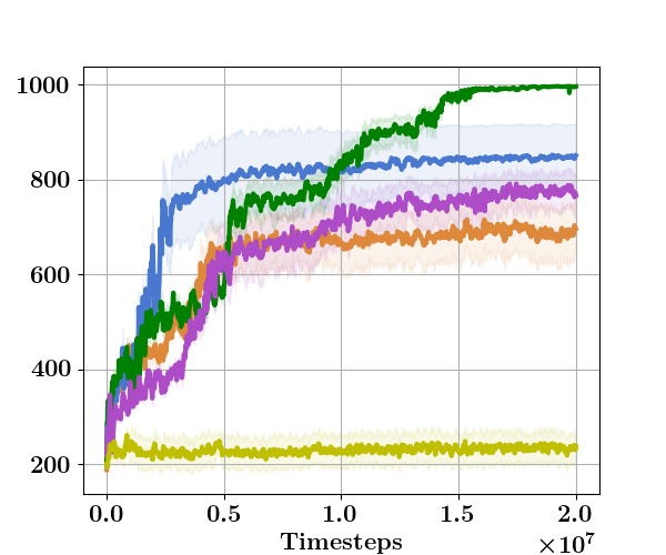
(a) Balance (DM)

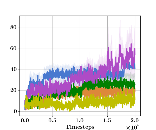
(b) Pendulum (DM)

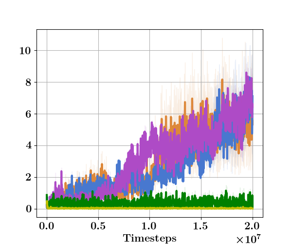
(c) HopperHop (DM)

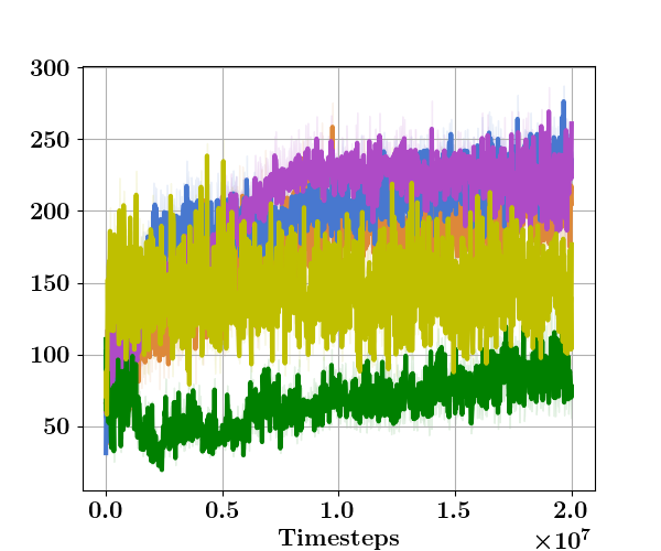
(d) AntWalk(DM)

Figure 3: Training performance on Continuous Control Benchmarks: Swimmer, HalfCheetah, CartPole $+$ $\{\text{Swingup},\text{TwoPoles},\text{Balance}\}$, Pendulum Swingup, Cheetah Run and Hopper. Tasks with DM stickers are from the DeepMind Control Suites. We compare five alternatives: baseline ES (orange), CV (blue, ours), ORTHO (marron), GCMC (green) and QMC (yellow). Each task is trained for $2\cdot 10^{7}$ time steps (LQR is trained for $4\cdot 10^{6}$ steps) and the training curves show the mean $\pm$ std cumulative rewards across 5 random seeds.

D.2 Discussion on Policy Gradient Methods

Instability of pg.

It has been observed that the vanilla pg estimators are not stable. Even when the discount factor $\gamma<1$ is introduced to reduce the variance, vanilla pg estimators can still have large variance due to the long horizon. As a result in practice, the original form of the pg (5) is rarely used. Instead, prior works and practical implementations tend to introduce bias into the estimators in exchange for lower variance: e.g. average across states intsead of trajectories (Dhariwal et al., 2017), clipping based trust region (Schulman et al., 2017) and biased advantage estimation (Schulman et al., 2016). These techniques stabilize the estimator and lead to state-of-the-art performance, however, their theoretical property is less clear (due to their bias). We leave the study of combining such biased estimators with es as future work.

D.3 Additional Results with TRPO/PPO and Deterministic Policies

We provide additional comparison results against TRPO/PPO and deterministic policies in Table 3. We see that generally TRPO/PPO achieve better performance, yet are still under-performed by CV. On the other hand, though deterministic policies tend to outperform stochastic policies when combined with the es baselines, they are not as good as stochastic policies with CV.

Comparison of implementation variations of pg algorithms.

Note that for fair comparison, we remove certain functionalities of a full fledged pg implementation as in (Dhariwal et al., 2017). We identify important differences between our baseline and the full fledged implementation and evaluate their effects on the performance in Table 4. Our analysis focuses on PPO. These important implementation differences are

• S: Normalization of observations.

• A: Normalization of advantages.

• M: Multiple gradient updates (in particular, $10$ gradient updates), instead of $1$ for our baseline.

To understand results in Table 4, we start with the notations of variations of PPO implementations. The PPO denotes our baseline for comparison; the PPO+S denotes our baseline with observation normalization. Similarly, we have PPO+A and PPO+M. Notations such as PPO+S+A denote the composition of these implementation techniques. We evaluate these implementation variations on a subset of tasks and compare their performance in Table 4.

We make several observations: (1) Multiple updates bring the most significant for pg. While conventional es implementations only consider one gradient update per iteration (Salimans et al., 2017), it is likely that they coudl also benefit from this modification; (2) Even when considering these improvements, our proposed CV method still outperforms pg baselines on a number of tasks.

Appendix E Discussion on Scalability

es easily scale to a large distributed architecture for the trajectory collection (Salimans et al., 2017; Mania et al., 2018). Indeed, the bottleneck of most es applications seem to be the sample collection, which can be conveniently distributed across multiple cores (machines). Fortunately, many open source implementations have provided high-quality packages via efficient inter-process communications and various techniques to reduce overheads (Salimans et al., 2017; Mania et al., 2018).

On the other hand, distributing pg requires more complicated software design. Indeed, distributed pg involve both distributed sample collection and gradient computations. The challenge lies in how to construct gradients via multiple processes and combine them into a single update, without introducing costly overheads. Open source implementations such as (Dhariwal et al., 2017) have achieved synchronized distributed gradient computations via MPI.

To scale CV, we need to combine both distributed sample collection from es and distributed gradient computation from pg. Since both of the above two components have been implemented with high quality via open source packages, we expect it not to be a big issue to scale CV, in particular to combine scalable gradient computation with es. However, this requires additional efforts - as these two parts have never been organically combined before and there is so far little (open source) engineering effort into this domain. We leave this as future work.

Table 3: Final performance on benchmark tasks. The policy is trained for a fixed number of steps on each task. The result is $\text{mean}\pm\text{std}$ across 5 random seeds. The best results are highlighted in bold font. We highlight multiple methods if their results cannot be separated ($\text{mean}\pm\text{std}$ overlap). CV (ours) achieves consistent gains over the baseline and other variance reduction methods. We also include a pg baseline.

Tasks	PPO	TRPO	Det	CV (Ours)	PG
Swimmer	$11\pm 7$	$11\pm 7$	$191\pm 100$	$\mathbf{237\pm 33}$	$-132\pm 5$
HalfCheetah	$-175\pm 20$	$-174\pm 16$	$1645\pm 1298$	$\mathbf{1897\pm 232}$	$-180\pm 4$
Walker	$657\pm 291$	$657\pm 292$	$1588\pm 744$	$\mathbf{1476\pm 112}$	$282\pm 25$
Pong(R)	$-17.1\pm 0.4$	$-15.0\pm 2.6$	$-10.4\pm 5.4$	$\mathbf{-3.0\pm 0.3}$	$-17\pm 0.2$
HalfCheetah(R)	$14\pm 2$	$13\pm 3$	$502\pm 199$	$\mathbf{709\pm 16}$	$12\pm 0$
BipedalWalker	$-66\pm 39$	$-66\pm 38$	$1\pm 2$	$\mathbf{105\pm 40}$	$-82\pm 12$
Cheetah(DM)	$20\pm 20$	$36\pm 32$	$241\pm 47$	$\mathbf{296\pm 15}$	$25\pm 6$
Pendulum(DM)	$0.6\pm 0.5$	$7.5\pm 4.8$	$40\pm 16$	$\mathbf{43\pm 1}$	$3\pm 1$
TwoPoles(DM)	$264\pm 46$	$42\pm 52$	$190\pm 58$	$\mathbf{245\pm 29}$	$14\pm 1$
Balance(DM)	$264\pm 46$	$515\pm 42$	$692\pm 250$	$\mathbf{847\pm 71}$	$401\pm 12$
HopperHop(DM)	$0.2\pm 0.2$	$0.0\pm 0.0$	$4.6\pm 6.2$	$\mathbf{6.5\pm 1.5}$	$0.1\pm 0.0$
AntWalk(DM)	$96\pm 36$	$180\pm 41$	$192\pm 20$	$\mathbf{239\pm 10}$	$100\pm 11$
AntEscape(DM)	$6\pm 3$	$10\pm 1$	$13\pm 8$	$\mathbf{51\pm 2}$	$6\pm 1$

Table 4: Evaluation of implementation variations of pg methods, with comparison to the CV. Below show the final performances on benchmark tasks. The policy is trained for a fixed number of steps on each task. The result below shows the mean performance averaged across 3 random seeds. The best results are highlighted in bold font. Notice below the table is transposed due to space.

Tasks	Swimmer	HalfCheetah	Pendulum	Balance	Hopper	AntWalk
PPO	$11$	$-175$	$0.6$	$264$	$0.2$	$96$
PPO+S	$30$	$126$	$2$	$308$	$0.5$	$80$
PPO+A	$33$	$67$	$26$	$278$	$0.4$	$117$
PPO+S+A	$31$	$192$	$1$	$386$	$0.6$	$106$
PPO+S+M	$110$	$1579$	$36$	$652$	$0.3$	$180$
PPO+A+M	$51$	$\mathbf{2414}$	$\mathbf{223}$	$771$	$46$	$173$
PPO+S+A+M	$106$	$1528$	$17$	$750$	$\mathbf{46.4}$	$144$
CV(Ours)	$\mathbf{237}$	$1897$	$43$	$\mathbf{847}$	$6.5$	$\mathbf{239}$

References

- Brockman et al. (2016) Brockman, G., Cheung, V., Pettersson, L., Schneider, J., Schulman, J., Tang, J., and Zaremba, W. (2016). Openai gym. arXiv preprint arXiv:1606.01540.
- Choromanski et al. (2018) Choromanski, K., Rowland, M., Sindhwani, V., Turner, R., and Weller, A. (2018). Structured evolution with compact architectures for scalable policy optimization. In Dy, J. and Krause, A., editors, Proceedings of the 35th International Conference on Machine Learning, volume 80 of Proceedings of Machine Learning Research, pages 970–978, Stockholmsmässan, Stockholm Sweden. PMLR.
- Dhariwal et al. (2017) Dhariwal, P., Hesse, C., Klimov, O., Nichol, A., Plappert, M., Radford, A., Schulman, J., Sidor, S., and Wu, Y. (2017). Openai baselines. https://github.com/openai/baselines.
- Grathwohl et al. (2018) Grathwohl, W., Choi, D., Wu, Y., Roeder, G., and Duvenaud, D. (2018). Backpropagation through the void: Optimizing control variates for black-box gradient estimation. In International Conference on Learning Representations.
- Gu et al. (2016) Gu, S., Levine, S., Sutskever, I., and Mnih, A. (2016). Muprop: Unbiased backpropagation for stochastic neural networks. In 4th International Conference on Learning Representations (ICLR).
- Gu et al. (2017) Gu, S., Lillicrap, T., Ghahramani, Z., Turner, R. E., and Levine, S. (2017). Q-prop: Sample-efficient policy gradient with an off-policy critic. In Proceedings International Conference on Learning Representations (ICLR). OpenReviews.net.
- Jang et al. (2017) Jang, E., Gu, S., and Poole, B. (2017). Categorical reparameterization with gumbel-softmax. In International Conference on Learning Representations.
- Kingma and Ba (2014) Kingma, D. P. and Ba, J. (2014). Adam: A method for stochastic optimization. arXiv preprint arXiv:1412.6980.
- Kingma and Welling (2014) Kingma, D. P. and Welling, M. (2014). Auto-encoding variational bayes. In International Conference on Learning Representations.
- Leordeanu and Hebert (2008) Leordeanu, M. and Hebert, M. (2008). Smoothing-based optimization. In 2008 IEEE Conference on Computer Vision and Pattern Recognition, pages 1–8. IEEE.
- Liu et al. (2017) Liu, H., Feng, Y., Mao, Y., Zhou, D., Peng, J., and Liu, Q. (2017). Action-depedent control variates for policy optimization via stein’s identity. arXiv preprint arXiv:1710.11198.
- Maddison et al. (2017) Maddison, C. J., Mnih, A., and Teh, Y. W. (2017). The concrete distribution: a continuous relaxation of discrete random variables. In International Conference on Learning Representations.
- Mania et al. (2018) Mania, H., Guy, A., and Recht, B. (2018). Simple random search of static linear policies is competitive for reinforcement learning. In Bengio, S., Wallach, H., Larochelle, H., Grauman, K., Cesa-Bianchi, N., and Garnett, R., editors, Advances in Neural Information Processing Systems 31, pages 1800–1809. Curran Associates, Inc.
- Mnih et al. (2016) Mnih, V., Badia, A. P., Mirza, M., Graves, A., Lillicrap, T., Harley, T., Silver, D., and Kavukcuoglu, K. (2016). Asynchronous methods for deep reinforcement learning. In International Conference on Machine Learning, pages 1928–1937.
- Paisley et al. (2012) Paisley, J. W., Blei, D. M., and Jordan, M. I. (2012). Variational bayesian inference with stochastic search. In ICML. icml.cc / Omnipress.
- Ranganath et al. (2014) Ranganath, R., Gerrish, S., and Blei, D. (2014). Black box variational inference. In Artificial Intelligence and Statistics, pages 814–822.
- Robbins and Monro (1951) Robbins, H. and Monro, S. (1951). A stochastic approximation method. The Annals of Mathematical Statistics.
- Ross (2002) Ross, S. (2002). Simulation, 2002.
- Rowland et al. (2018) Rowland, M., Choromanski, K. M., Chalus, F., Pacchiano, A., Sarlos, T., Turner, R. E., and Weller, A. (2018). Geometrically coupled monte carlo sampling. In Advances in Neural Information Processing Systems, pages 195–206.
- Salimans et al. (2017) Salimans, T., Ho, J., Chen, X., Sidor, S., and Sutskever, I. (2017). Evolution strategies as a scalable alternative to reinforcement learning. arXiv preprint arXiv:1703.03864.
- Schulman et al. (2015a) Schulman, J., Heess, N., Weber, T., and Abbeel, P. (2015a). Gradient estimation using stochastic computation graphs. In Advances in Neural Information Processing Systems, pages 3528–3536.
- Schulman et al. (2015b) Schulman, J., Levine, S., Abbeel, P., Jordan, M., and Moritz, P. (2015b). Trust region policy optimization. In International Conference on Machine Learning, pages 1889–1897.
- Schulman et al. (2016) Schulman, J., Moritz, P., Levine, S., Jordan, M., and Abbeel, P. (2016). High-dimensional continuous control using generalized advantage estimation. In Proceedings of the International Conference on Learning Representations (ICLR).
- Schulman et al. (2017) Schulman, J., Wolski, F., Dhariwal, P., Radford, A., and Klimov, O. (2017). Proximal policy optimization algorithms. arXiv preprint arXiv:1707.06347.
- Silver et al. (2014) Silver, D., Lever, G., Heess, N., Degris, T., Wierstra, D., and Riedmiller, M. (2014). Deterministic policy gradient algorithms. In ICML.
- Sutton et al. (2000) Sutton, R. S., McAllester, D. A., Singh, S. P., and Mansour, Y. (2000). Policy gradient methods for reinforcement learning with function approximation. In Advances in neural information processing systems, pages 1057–1063.
- Tassa et al. (2018) Tassa, Y., Doron, Y., Muldal, A., Erez, T., Li, Y., Casas, D. d. L., Budden, D., Abdolmaleki, A., Merel, J., Lefrancq, A., et al. (2018). Deepmind control suite. arXiv preprint arXiv:1801.00690.
- Tokui et al. (2015) Tokui, S., Oono, K., Hido, S., and Clayton, J. (2015). Chainer: a next-generation open source framework for deep learning. In Proceedings of workshop on machine learning systems (LearningSys) in the twenty-ninth annual conference on neural information processing systems (NIPS), volume 5, pages 1–6.
- Tucker et al. (2018) Tucker, G., Bhupatiraju, S., Gu, S., Turner, R., Ghahramani, Z., and Levine, S. (2018). The mirage of action-dependent baselines in reinforcement learning. In Dy, J. and Krause, A., editors, Proceedings of the 35th International Conference on Machine Learning, volume 80 of Proceedings of Machine Learning Research, pages 5015–5024, Stockholmsmässan, Stockholm Sweden. PMLR.
- Tucker et al. (2017) Tucker, G., Mnih, A., Maddison, C. J., Lawson, J., and Sohl-Dickstein, J. (2017). Rebar: Low-variance, unbiased gradient estimates for discrete latent variable models. In Advances in Neural Information Processing Systems, pages 2627–2636.
- Wu et al. (2018) Wu, C., Rajeswaran, A., Duan, Y., Kumar, V., Bayen, A. M., Kakade, S., Mordatch, I., and Abbeel, P. (2018). Variance reduction for policy gradient with action-dependent factorized baselines. In International Conference on Learning Representations.