Neural Stored-program Memory

Abstract

Neural networks powered with external memory simulate computer behaviors. These models, which use the memory to store data for a neural controller, can learn algorithms and other complex tasks. In this paper, we introduce a new memory to store weights for the controller, analogous to the stored-program memory in modern computer architectures. The proposed model, dubbed Neural Stored-program Memory, augments current memory-augmented neural networks, creating differentiable machines that can switch programs through time, adapt to variable contexts and thus resemble the Universal Turing Machine. A wide range of experiments demonstrate that the resulting machines not only excel in classical algorithmic problems, but also have potential for compositional, continual, few-shot learning and question-answering tasks.

1 Introduction

Recurrent Neural Networks (RNNs) are Turing-complete Siegelmann & Sontag (1995). However, in practice RNNs struggle to learn simple procedures as they lack explicit memory Graves et al. (2014); Mozer & Das (1993). These findings have sparked a new research direction called Memory Augmented Neural Networks (MANNs) that emulate modern computer behavior by detaching memorization from computation via memory and controller network, respectively. MANNs have demonstrated significant improvements over memory-less RNNs in various sequential learning tasks Graves et al. (2016); Le et al. (2018a); Sukhbaatar et al. (2015). Nonetheless, MANNs have barely simulated general-purpose computers.

Current MANNs miss a key concept in computer design: stored-program memory. The concept has emerged from the idea of Universal Turing Machine (UTM) Turing (1936) and further developed in Harvard Architecture Broesch (2009), Von Neumann Architecture von Neumann (1993). In UTM, both data and programs that manipulate the data are stored in memory. A control unit then reads the programs from the memory and executes them with the data. This mechanism allows flexibility to perform universal computations. Unfortunately, current MANNs such as Neural Turing Machine (NTM) Graves et al. (2014), Differentiable Neural Computer (DNC) Graves et al. (2016) and Least Recently Used Access (LRUA) Santoro et al. (2016) only support memory for data and embed a single program into the controller network, which goes against the stored-program memory principle.

Our goal is to advance a step further towards UTM by coupling a MANN with an external program memory. The program memory co-exists with the data memory in the MANN, providing more flexibility, reuseability and modularity in learning complicated tasks. The program memory stores the weights of the MANN’s controller network, which are retrieved quickly via a key-value attention mechanism across timesteps yet updated slowly via backpropagation. By introducing a meta network to moderate the operations of the program memory, our model, henceforth referred to as Neural Stored-program Memory (NSM), can learn to switch the programs/weights in the controller network appropriately, adapting to different functionalities aligning with different parts of a sequential task, or different tasks in continual and few-shot learning.

To validate our proposal, the NTM armed with NSM, namely Neural Universal Turing Machine (NUTM), is tested on a variety of synthetic tasks including algorithmic tasks from Graves et al. (2014), composition of algorithmic tasks and continual procedure learning. For these algorithmic problems, we demonstrate clear improvements of NUTM over NTM. Further, we investigate NUTM in few-shot learning by using LRUA as the MANN and achieve notably better results. Finally, we expand NUTM application to linguistic problems by equipping NUTM with DNC core and achieve competitive performances against state-of-the-arts in the bAbI task Weston et al. (2015).

Taken together, our study advances neural network simulation of Turing Machines to neural architecture for Universal Turing Machines. This develops a new class of MANNs that can store and query both the weights and data of their own controllers, thereby following the stored-program principle. A set of five diverse experiments demonstrate the computational universality of the approach.

2 Background

In this section, we briefly review MANN and its relations to Turing Machines. A MANN consists of a controller network and an external memory $\mathbf{M}\in\mathbb{R}^{N\times M}$, which is a collection of $N$ $M$-dimensional vectors. The controller network is responsible for accessing the memory, updating its state and optionally producing output at each timestep. The first two functions are executed by an interface network and a state network, respectively. Usually, the interface network is a Feedforward neural network whose input is $c_{t}$ - the output of the state network implemented as RNNs. Let $W^{c}$ denote the weight of the interface network, then the state update and memory control are as follows,

$$h_{t},c_{t}=RNN\left(\left[x_{t},r_{t-1}\right],h_{t-1}\right)$$ (1)

$$\xi_{t}=c_{t}W^{c}$$ (2)

where $x_{t}$ and $r_{t-1}$ are data from current input and the previous memory read, respectively. The interface vector $\xi_{t}$ then is used to read from and write to the memory $\mathbf{M}$. We use a generic notation $memory\left(\xi_{t},\mathbf{M}\right)$ to represent these memory operations that either update or retrieve read value $r_{t}$ from the memory. To support multiple memory accesses per step, the interface network may produce multiple interfaces, also known as control heads. Readers are referred to App. F and Graves et al. (2014; 2016); Santoro et al. (2016) for details of memory read/write examples.

A deterministic one-tape Turing Machine can be defined by 4-tuple $\left(Q,\Gamma,\delta,q_{0}\right)$, in which $Q$ is finite set of states, $q_{0}\in Q$ is an initial state, $\Gamma$ is finite set of symbol stored in the tape (the data) and $\delta$ is the transition function (the program), $\delta:Q\times\Gamma\rightarrow\Gamma\times\left\{-1,1\right\}\times Q$. At each step, the machine performs the transition function, which takes the current state and the read value from the tape as inputs and outputs actions including writing new values, moving tape head to new location (left/right) and jumping to another state. Roughly mapping to current MANNs, $Q$, $\Gamma$ and $\delta$ map to the set of the controller states, the read values and the controller network, respectively. Further, the function $\delta$ can be factorized into two sub functions: $Q\times\Gamma\rightarrow\Gamma\times\left\{-1,1\right\}$ and $Q\times\Gamma\rightarrow Q$, which correspond to the interface and state networks, respectively.

By encoding a Turing Machine into the tape, one can build a UTM that simulates the encoded machine Turing (1936). The transition function $\delta_{u}$ of the UTM queries the encoded Turing Machine that solves the considering task. Amongst 4 tuples, $\delta$ is the most important and hence uses most of the encoding bits. In other words, if we assume that the space of $Q$, $\Gamma$ and $q_{0}$ are shared amongst Turing Machines, we can simulate any Turing Machine by encoding only its transition function $\delta$. Translating to neural language, if we can store the controller network into a queriable memory and make use of it, we can build a Neural Universal Turing Machine. Using NSM is a simple way to achieve this goal, which we introduce in the subsequent section.

3 Methods

3.1 Neural Stored-program Memory

A Neural Stored-program Memory (NSM) is a key-value memory $\mathbf{M}_{p}\in\mathbb{R}^{P\times(K+S)}$, whose values are the basis weights of another neural network$-$the programs. $P$, $K$, and $S$ are the number of programs, the key space dimension and the program size, respectively. This concept is a hybrid between the traditional slow-weight and fast-weight Hinton & Plaut (1987). Like slow-weight, the keys and values in NSM are updated gradually by backpropagation. However, the values are dynamically interpolated to produce the working weight on-the-fly during the processing of a sequence, which resembles fast-weight computation. Let us denote $\mathbf{M}_{p}\left(i\right).k$ and $\mathbf{M}_{p}\left(i\right).v$ as the key and the program of the $i$-th memory slot. At timestep $t,$ given a query key $k_{t}^{p}$, the working program is retrieved as follows,

$$D\left(k_{t}^{p},\mathbf{M}_{p}(i).k\right)=\frac{k_{t}^{p}\cdot\mathbf{M}_{p}(i).k}{||k_{t}^{p}||\cdot||\mathbf{M}_{p}(i).k)||}$$ (3)

$$w_{t}^{p}\left(i\right)=\text{softmax}\left(\beta_{t}^{p}D\left(k_{t}^{p},\mathbf{M}_{p}(i).k\right)\right)$$ (4)

$$p_{t}=\stackrel{{\scriptstyle[}}{{i}}=1]{P}{\sum}w_{t}^{p}\left(i\right)\mathbf{M}_{p}\left(i\right).v$$ (5)

where $D\left(\cdot\right)$ is cosine similarity and $\beta_{t}^{p}$ is the scalar program strength parameter. The vector working program $p_{t}$ is then reshaped to its matrix form and ready to be used as the weight of other neural networks.

The key-value design is essential for convenient memory access as the size of the program stored in $\mathbf{M}_{p}$ can be millions of dimensions and thus, direct content-based addressing as in Graves et al. (2014; 2016); Santoro et al. (2016) is infeasible. More importantly, we can inject external control on the behavior of the memory by imposing constraints on the key space. For example, program collapse will happen when the keys stored in the memory stay close to each other. When this happens, $p_{t}$ is a balanced mixture of all programs regardless of the query key and thus having multiple programs is useless. We can avoid this phenomenon by minimizing a regularization loss defined as the following,

$$l_{p}=\stackrel{{\scriptstyle[}}{{i}}=1]{P}{\sum}\stackrel{{\scriptstyle[}}{{j}}=i+1]{P}{\sum}D\left(\mathbf{M}_{p}(i).k,\mathbf{M}_{p}(j).k\right)$$ (6)

3.2 Neural Universal Turing Machine

It turns out that the combination of MANN and NSM approximates a Universal Turing Machine (Sec. 2). At each timestep, the controller in MANN reads its state and memory to generate control signal to the memory via the interface network $W^{c}$, then updates its state using the state network $RNN$. Since the parameters of $RNN$ and $W^{c}$ represent the encoding of $\delta$, we should store both into NSM to completely encode an MANN. For simplicity, in this paper, we only use NSM to store $W^{c}$, which is equivalent to the Universal Turing Machine that can simulate any one-state Turing Machine.

In traditional MANN, $W^{c}$ is constant across timesteps and only updated slowly during training, typically through backpropagation. In our design, we compute $W_{t}^{c}$ from NSM for every timestep and thus, we need a program interface network$-$the meta network $P_{\mathscr{\mathcal{I}}}-$that generates an interface vector for the program memory: $\xi_{t}^{p}=P_{\mathscr{\mathcal{I}}}\left(c_{t}\right)$, where $\xi_{t}^{p}=\left[k_{t}^{p},\beta_{t}^{p}\right]$. Together with the $RNN$, $P_{\mathscr{\mathcal{I}}}$ simulates $\delta_{u}$ of the UTM and is implemented as a Feedforward neural network. The procedure for computing $W_{t}^{c}$ is executed by following Eqs. (3)-(5), hereafter referred to as $NSM\left(\xi_{t}^{p},\mathbf{M}_{p}\right)$. Figure 1 depicts the integration of NSM into MANN.

In this implementation, key-value NSM offers a more flexible learning scheme than direct attention, in which the meta-network can generate the weight $w_{t}^{p}$ directly without matching $k_{t}^{p}$ with $\mathbf{M}_{p}\left(i\right).k$. That is, only the meta-network learns the mapping from context $c_{t}$ to program. When it falls into some local-minima (generating suboptimal $w_{t}^{p}$), the meta-network struggles to escape. In our proposal, together with the meta-network, the memory keys are learnable. When the memory keys are slowly updated, the meta-network will shift its query key generation to match the new memory keys and possibly escape from the local-minima.

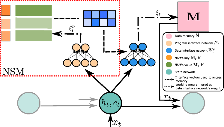
Figure 1: Introducing NSM into MANN. At each timestep, the program interface network ($P_{\mathscr{\mathcal{I}}}$) receives input from the state network and queries the program memory $\mathbf{M}_{p}$, acquiring the working weight for the interface network ($W_{t}^{c}$). The interface network then operates on the data memory $\mathbf{M}$.

For the case of multi-head NTM, we implement one NSM per control head and name this model Neural Universal Turing Machine (NUTM). One NSM per head is to ensure programs for one head do not interfere with other heads and thus, encourage functionality separation amongst heads. Each control head will read from (for read head) or write to (for write head) the data memory $\mathbf{M}$ via $memory\left(\xi_{t},\mathbf{M}\right)$ as described in Graves et al. (2014) . It should be noted that using multiple heads is unlike using multiple controllers per head. The former increases the number of accesses to the data memory at each timestep and employs a fixed controller to compute multiple heads, which may improve capacity yet does not enable adaptability. On the contrary, the latter varies the property of each memory access across timesteps by switching the controllers and thus potential for adaptation.

Other MANNs such as DNC Graves et al. (2016) and LRUA Santoro et al. (2016) can be armed with NSM in this manner. We also employ the regularization loss $l_{p}$ to prevent the programs from collapsing, resulting in a final loss as follows,

$$Loss=Loss_{pred}+\eta_{t}l_{p}$$ (7)

where $Loss_{pred}$ is the prediction loss and $\eta_{t}$ is annealing factor, reducing as the training step increases. The details of NUTM operations are presented in Algorithm 1.

1:a sequence $x=\left\{x_{t}\right\}_{t=1}^{T}$, a data memory $\mathbf{M}$ and $R$ program memories $\left\{\mathbf{M}_{p,n}\right\}_{n=1}^{R}$ corresponding to $R$ control heads

2:Initilize $h_{0}$, $r_{0}$

3:for $t=1,T$ do

4:     $h_{t},c_{t}=RNN([x_{t},r_{t-1}],h_{t-1})$ $\triangleright$ $RNN$ can be replaced by GRU/LSTM

5:     for $n=1,R$ do

6:         Compute the program interface $\xi_{t,n}^{p}\leftarrow P_{\mathscr{\mathcal{I}},n}\left(c_{t}\right)$

7:         Compute the program $W_{t,n}^{c}\leftarrow NSM\left(\xi_{t,n}^{p},\mathbf{M}_{p,n}\right)$

8:         Compute the data interface $\xi_{t,n}\leftarrow c_{t}W_{t,n}^{c}$

9:          Read $r_{t,n}$ from memory $\mathbf{M}$ (if read head) or update memory $\mathbf{M}$ (if write head) using $memory_{n}(\xi_{t,n},\mathbf{M})$

10:     end for

11:     $r_{t}\leftarrow\left[r_{t,1},...,r_{t,R}\right]$

12:end for

Algorithm 1 Neural Universal Turing Machine

3.3 On the Benefit of NSM to MANN: An Explanation from Multilevel Modeling

Learning to access memory is a multi-dimensional regression problem. Given the input $c_{t}$, which is derived from the state $h_{t}$ of the controller, the aim is to generate a correct interface vector $\xi_{t}$ via optimizing the interface network. Instead of searching for one transformation that maps the whole space of $c_{t}$ to the optimal space of $\xi_{t}$, NSM first partitions the space of $c_{t}$ into subspaces, then finds multiple transformations, each of which covers subspace of $c_{t}$. The program interface network $P_{\mathscr{\mathcal{I}}}$ is a meta learner that routes $c_{t}$ to the appropriate transformation, which then maps $c_{t}$ to the $\xi_{t}$ space. This is analogous to multilevel regression in statistics Andrew Gelman (2006). Practical studies have shown that multilevel regression is better than ordinary regression if the input is clustered Cohen et al. (2014); Huang (2018).

RNNs have the capacity to learn to perform finite state computations Casey (1996); Tiňo et al. (1998). The states of a RNN must be grouped into partitions representing the states of the generating automaton. As Turing Machines are finite state automata augmented with an external memory tape, we expect MANN, if learnt well, will organize its state space clustered in a way to reflect the states of the emulated Turing Machine. That is, $h_{t}$ as well as $c_{t}$ should be clustered. We realize that NSM helps NTM learn better clusterization over this space (see App. A), thereby improving NTM’s performances.

4 Results

4.1 NTM Single Tasks

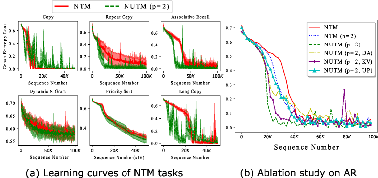
Figure 2: Learning curves on NTM tasks (a) and Associative Recall (AR) ablation study (b). Only mean is plotted in (b) for better visualization.

Task	Copy	R. Copy	A. Recall	D. N-grams	P. Sort	L. Copy
NTM	0.00	405.10	7.66	132.59	24.41	16.04
NUTM (p=2)	0.00	366.69	1.35	127.68	20.00	0.02

Table 1: Generalization performance of best models measured in average bit error per sequence (lower is better). For each task, we pick 1,000 longer sequences as test data.

In this section, we investigate the performance of NUTM on algorithmic tasks introduced in Graves et al. (2014) : Copy, Repeat Copy, Associative Recall, Dynamic N-Grams and Priority Sort. Besides these five NTM tasks, we add another task named Long Copy which doubles the length of training sequences in the Copy task. In these tasks, the model will be fed a sequence of input items and is required to infer a sequence of output items. Each item is represented by a binary vector.

In the experiment, we compare two models: NTM and NUTM with two programs. Although the tasks are atomic, we argue that there should be at least two memory manipulation schemes across timesteps, one for encoding the inputs to the memory and another for decoding the output from the memory. The two models are trained with cross-entropy objective function under the same setting as in Graves et al. (2014) . For fair comparison, the controller hidden dimension of NUTM is set smaller to make the total number of parameters of NUTM equivalent to that of NTM. The number of memory heads for both models are always equal and set to the same value as in the original paper (details in App. C).

We run each experiments five times and report the mean with error bars of training losses for NTM tasks in Fig. 2 (a). Except for the Copy task, which is too simple, other tasks observe convergence speed improvement of NUTM over that of NTM, thereby validating the benefit of using two programs across timesteps even for the single task setting. NUTM requires fewer training samples to converge and it generalizes better to unseen sequences that are longer than training sequences. Table 1 reports the test results of the best models chosen after five runs and confirms the outperformance of NUTM over NTM for generalization.

To illustrate the program usage, we plot NUTM’s program distributions across timesteps for Repeat Copy and Priority Sort in Fig. 3 (a) and (b), respectively. Examining the read head for Repeat Copy, we observe two program usage patterns corresponding to the encoding and decoding phases. As there is no reading in encoding, NUTM assigns the “no-read” strategy mainly to the “orange program”. In decoding, the sequential reading is mostly done by the “blue program” with some contributions from the “orange program” when resetting reading head. Similar behaviors can be found in the write head for Priority Sort. While the encoding “fitting writing” (see Graves et al. (2014) for explanation on the strategy) is often executed by the “blue program”, the decoding writing is completely taken by the “orange” program (more visualizations in App. B).

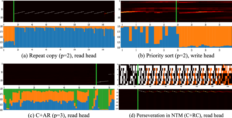
Figure 3: (a,b,c) visualizes NUTM’s executions in synthetic tasks: the upper rows are memory read (left)/write (right) locations; the lower rows are program distributions over timesteps. The green line indicates the start of the decoding phase. (d) visualizes perseveration in NTM: the upper row are input, output, predicted output with errors (orange bits); the lower row is reading location.

4.2 Ablation study on Associative Recall

In this section, we conduct an ablation study on Associative Recall (AR) to validate the benefit of proposed components that constitute NSM. We run the task with three additional baselines: NUTM using direct attention (DA), NUTM using key-value without regularization (KV), NUTM using fixed, uniform program distribution (UP) and a vanilla NTM with 2 memory heads ($h=2$). The meta-network $P_{\mathscr{\mathcal{I}}}$ in DA generates the attention weight $w_{t}^{p}$ directly. The KV employs key-value attention yet excludes the regularization loss presented in Eq. (6). The training curves over 5 runs are plotted in Fig. 2 (b). The results demonstrate that DA exhibits fast yet shallow convergence. It tends to fall into local minima, which finally fails to reach zero loss. Key-value attention helps NUTM converge completely with fewer iterations. The performance is further improved with the proposed regularization loss. UP underperforms NUTM as it lacks dynamic programs. The NTM with 2 heads shows slightly better convergence compared to the NTM, yet obviously underperforms NUTM ($p=2$) with 1 head and fewer parameters. This validates our argument on the difference between using multiple heads and multiple programs (Sec. 3.2).

4.3 NTM Sequencing Tasks

In neuroscience, sequencing tasks test the ability to remember a series of tasks and switch tasks alternatively Blumenfeld (2010). A dysfunctional brain may have difficulty in changing from one task to the next and get stuck in its preferred task (perseveration phenomenon). To analyze this problem in NTM, we propose a new set of experiments in which a task is generated by sequencing a list of subtasks. The set of subtasks is chosen from the NTM single tasks (excluding Dynamic N-grams for format discrepancy) and the order of subtasks in the sequence is dictated by an indicator vector put at the beginning of the sequence. Amongst possible combinations of subtasks, we choose {Copy, Repeat Copy}(C+RC), {Copy, Associative Recall} (C+AR), {Copy, Priority Sort} (C+PS) and all (C+RC+AC+PS). The learner observes the order indicator followed by a sequence of subtasks’ input items and is requested to consecutively produce the output items of each subtasks.

As shown in Fig. 4, some tasks such as Copy and Associative Recall, which are easy to solve if trained separately, become unsolvable by NTM when sequenced together. One reason is NTM fails to change the memory access behavior (perseveration). For examples, NTM keeps following repeat copy reading strategy for all timesteps in C+RC task (Fig. 3 (d)). Meanwhile, NUTM can learn to change program distribution when a new subtask appears in the sequence and thus ensure different accessing strategy per subtask (Fig. 3 (c)).

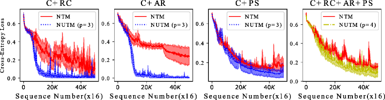
Figure 4: Learning curves on sequencing NTM tasks.

4.4 Continual Procedure Learning

In continual learning, catastrophic forgetting happens when a neural network quickly forgets previously acquired skills upon learning new skills French (1999). In this section, we prove the versatility of NSM by showing that a naive application of NSM without much modification can help NTM to mitigate catastrophic forgetting. We design an experiment similar to the Split MNIST Zenke et al. (2017) to investigate whether NSM can improve NTM’s performance. In our experiment, we let the models see the training data from the 4 tasks: Copy (C), Repeat Copy (RC), Associative Recall (AR) and Priority Sort (PS), consecutively in this order. Each task is trained in 20,000 iterations with batch size 16 (see App. C for task details). To encourage NUTM to spend exactly one program per task while freezing others, we force “hard” attention over the programs by replacing the softmax function in Eq. 5 with the Gumbel-softmax Jang et al. (2016). Also, to ignore catastrophic forgetting in the state network, we use Feedforward controllers in the two baselines.

After finishing one task, we evaluate the bit accuracy $-$measured by $1-$(bit error per sequence/total bits per sequence) over 4 tasks. As shown in in Fig. 5, NUTM outperforms NTM by a moderate margin (10-40% per task). Although NUTM also experiences catastrophic forgetting, it somehow preserves some memories of previous tasks. Especially, NUTM keeps performing perfectly on Copy even after it learns Repeat Copy. For other dissimilar task transitions, the performance drops significantly, which requires more effort to bring NSM to continual learning.

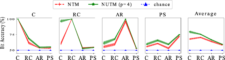
Figure 5: Mean bit accuracy with error bars for the continual algorithmic tasks. Each of the first four panels show bit accuracy on four tasks after finishing a task. The rightmost shows the average accuracy.

4.5 Few-shot Learning

Few-shot learning or meta learning tests the ability to rapidly adapt within a task while gradually capturing the way the task structure varies Thrun (1998). By storing sample-class bindings, MANNs are capable of classifying new data after seeing only few samples Santoro et al. (2016). As NSM gives flexible memory controls, it makes MANN more adaptive to changes and thus perform better in this setting. To verify that, we apply NSM to the LRUA memory and follow the experiments introduced in Santoro et al. (2016) , using the Omniglot dataset to measure few-shot classification accuracy. The dataset includes images of 1623 characters, with 20 examples of each character. During training, a sequence (episode) of images are randomly selected from $C$ classes of characters in the training set (1200 characters), where $C=5,10$ corresponding to sequence length of 50, 75, respectively. Each class is assigned a random label which shuffles between episodes and is revealed to the models after each prediction. After 100,000 episodes of training, the models are tested with unseen images from the testing set (423 characters). The two baselines are MANN and NUTM (both use LRUA core). For NUTM, we only tune $p$ and pick the best values: $p=2$ and $p=3$ for 5 classes and 10 classes, respectively.

Table 11 reports the classification accuracy when the models see characters for the second, third and fifth time. NUTM generally achieves better results than MANN, especially when the number of classes increases, demanding more adaptation within an episode. For the persistent memory mode, which demands fast forgetting old experiences in previous episodes, NUTM outperforms MANN significantly (10-20%). Readers are referred to App. D for more details on learning curves and more results of the models.

Model	Persistent	5 classes			10 classes
	memory	$2^{nd}$	$3^{rd}$	$5^{th}$	$2^{nd}$	$3^{rd}$	$5^{th}$
MANN (LRUA)*	No	82.8	91.0	94.9	-	-	-
MANN (LRUA)	No	82.3	88.7	92.3	52.7	60.6	64.7
NUTM (LRUA)	No	85.7	91.3	95.5	68.0	78.1	82.8
MANN (LRUA)	Yes	66.2	73.4	81.0	51.3	59.2	63.3
NUTM (LRUA)	Yes	77.8	85.8	89.8	69.0	77.9	82.7

Table 2: Test-set classification accuracy (%) on the Omniglot dataset after 100,000 episodes of training. * denotes available results from Santoro et al. (2016).

4.6 Text Question Answering

Reading comprehension typically involves an iterative process of multiple actions such as reading the story, reading the question, outputting the answers and other implicit reasoning steps Weston et al. (2015). We apply NUTM to the question answering domain by replacing the NTM core with DNC Graves et al. (2016). Compared to NTM’s sequential addressing, dynamic memory addressing in DNC is more powerful and thus suitable for NSM integration to solve non-algorithmic problems such as question answering. Following previous works of DNC, we use bAbI dataset Weston et al. (2015) to measure the performance of the NUTM with DNC core (three variants $p=1$, $p=2$ and $p=4$). In the dataset, each story is followed by a series of questions and the network reads all word by word, then predicts the answers. Although synthetically generated, bAbI is a good benchmark that tests 20 aspects of natural language reasoning including complex skills such as induction and counting,

We found that increasing number of programs helps NUTM improve performance. In particular, NUTM with 4 programs, after 50 epochs jointly trained on all 20 question types, can achieve a mean test error rate of 3.3% and manages to solve 19/20 tasks (a task is considered solved if its error <5%). The mean and s.d. across 10 runs are also compared with other results reported by recent works (see Table 3). Excluding baselines under different setups, our result is the best reported mean result on bAbI that we are aware of. More details are described in App. E.

Model	Error
DNCGraves et al. (2016)	16.7 ± 7.6
SDNCRae et al. (2016)	6.4 ± 2.5
ADNCFranke et al. (2018)	6.3 ± 2.7
DNC-MDCsordas & Schmidhuber (2019)	9.5 ± 1.6
NUTM (DNC core, p=1)	9.7 ± 3.5
NUTM (DNC core, p=2)	7.5 ± 1.6
NUTM (DNC core, p=4)	5.6 ± 1.9

Table 3: Mean and s.d. for bAbI error ($\%$).

5 Related Work

Previous investigations into MANNs mostly revolve around memory access mechanisms. The works in Graves et al. (2014; 2016) introduce content-based, location-based and dynamic memory reading/writing. Further, Rae et al. (2016) scales to bigger memory by sparse access; Le et al. (2019) optimizes memory operations with uniform writing; and MANNs with extra memory have been proposed Le et al. (2018b). However, these works keep using memory for storing data rather than the weights of the network and thus parallel to our approach. Other DNC modifications Csordas & Schmidhuber (2019); Franke et al. (2018) are also orthogonal to our work.

Another line of related work involves modularization of neural networks, which is designed for visual question answering. In module networks Andreas et al. (2016b; a), the modules are manually aligned with predefined concepts and the order of execution is decided by the question. Although the module in these works resembles the program in NSM, our model is more generic and flexible with soft-attention over programs and thus fully differentiable. Further, the motivation of NSM does not limit to a specific application. Rather, NSM aims to help MANN reach general-purpose computability.

If we view NSM network as a dynamic weight generator, the program in NSM can be linked to fast weight von der Malsburg (1981); Hinton & Plaut (1987); Schmidhuber (1993b). These papers share the idea of using different weights across timesteps to enable dynamic adaptation. Using outer-product is a common way to implement fast-weight Schmidhuber (1993a); Ba et al. (2016); Schlag & Schmidhuber (2017). These fast weights are directly generated and thus different from our programs, which are interpolated from a set of slow weights.

Tensor/Multiplicative RNN Sutskever et al. (2011) and Hypernetwork Ha et al. (2016) are also relevant related works. These methods attempt to make the working weight of RNNs dependent on the input to enable quick adaption through time. Nevertheless, they do not support modularity. In particular, Hypernetwork generates scaling factors for the single weight of the main RNN. It does not aim to use multiple slow-weights (programs) and thus, different from our approach. Tensor RNN is closer to our idea when the authors propose to store $M$ slow-weights, where $M$ is the number of input dimension, which is acknowledged impractical. Unlike our approach, they do not use a meta-network to generate convex combinations amongst weights. Instead, they propose Multiplicative RNN that factorizes the working weight to product of three matrices, which looses modularity. On the contrary, we explicitly model the working weight as an interpolation of multiple programs and use a meta-network to generate the coefficients. This design facilitates modularity because each program is trained towards some functionality and can be switched or combined with each other to perform the current task. Last but not least, while the related works focus on improving RNN with fast-weight, we aim to reach a neural simulation of Universal Turing Machine, in which fast-weight is a way to implement stored-program principle.

6 Conclusions

This paper introduces the Neural Stored-program Memory (NSM), a new type of external memory for neural networks. The memory, which takes inspirations from the stored-program memory in computer architecture, gives memory-augmented neural networks (MANNs) flexibility to change their control programs through time while maintaining differentiability. The mechanism simulates modern computer behavior, potential making MANNs truly neural computers. Our experiments demonstrated that when coupled with our model, the Neural Turing Machine learns algorithms better and adapts faster to new tasks at both sequence and sample levels. When used in few-shot learning, our method helps MANN as well. We also applied the NSM to the Differentiable Neural Computer and observed a significant improvement, reaching the state-of-the-arts in the bAbI task. Although this paper limits to MANN integration, other neural networks can also reap benefits from our proposed model, which will be explored in future works.

Appendix

A Clustering on The Latent Space

As previously mentioned in Sec. 3.3, MANN should let its states form clusters to well-simulate Turing Machine. Fig. 6 (a) and (c) show NTM actually organizes its $c_{t}$ space into clusters corresponding to processing states (e.g, encoding and decoding). NUTM, which explicitly partitions this space, clearly learn better clusters of $c_{t}$ (see Fig. 6 (b) and (d)). This contributes to NUTM’s outperformance over NTM.

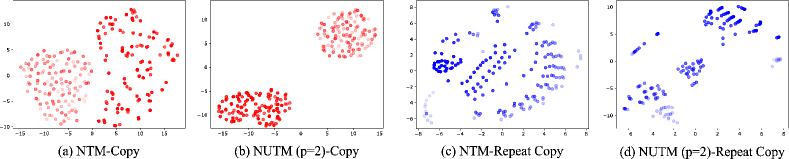
Figure 6: Visualization of the first two principal components of $c_{t}$ space in NTM (a,c) and NUTM (b,d) for Copy (red) and Repeat Copy (blue). Fader color denotes lower timestep in a sequence. Both can learn clusters of hidden states yet NUTM exhibits clearer partition.

B Program Usage Visualizations

B.1 and B.2 visualize the best inferences of NUTM on test data from single and sequencing tasks. Each plot starts with the input sequence and the predicted output sequence with error bits in the first row. The second and fourth rows depict the read and write locations on data memory, respectively. The third and fifth rows depict the program distribution of the read head and write head, respectively. B.3 visualizes random failed predictions of NTM on sequencing tasks. The plots follow previous pattern except for the program distribution rows.

B.1 Visualization on program distribution across timesteps (single tasks)

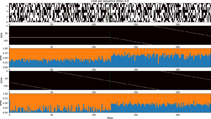
Figure 7: Copy (p=2).

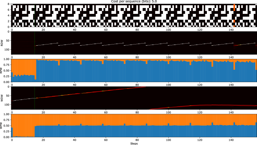
Figure 8: Repeat Copy (p=2).

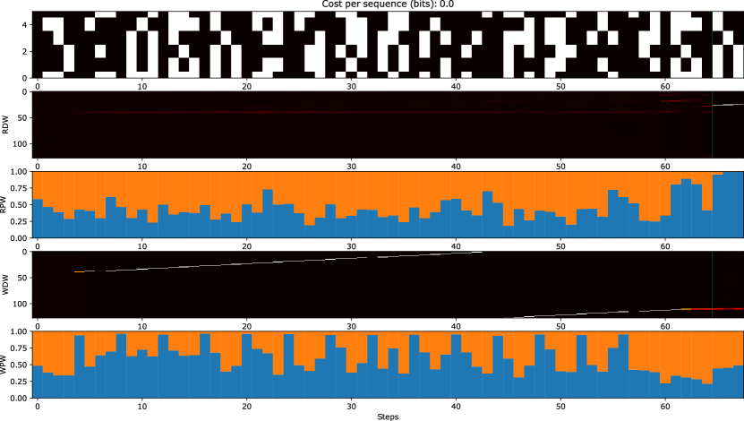
Figure 9: Associative Recall (p=2).

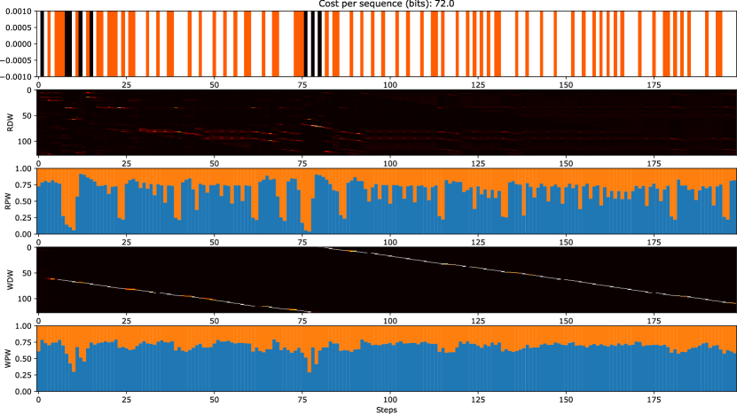
Figure 10: Dynamic N-grams (p=2).

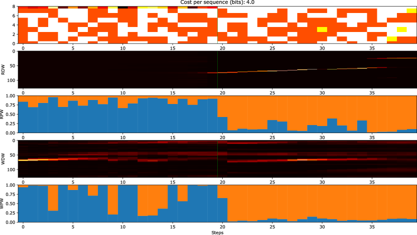
Figure 11: Priority Sort (p=2).

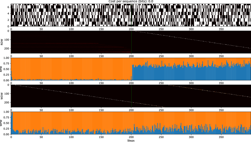
Figure 12: Long Copy (p=2).

B.2 Visualization on program distribution across timesteps (sequencing tasks)

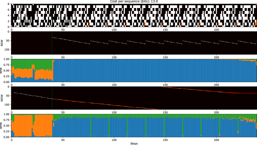
Figure 13: Copy+Repeat Copy (p=3).

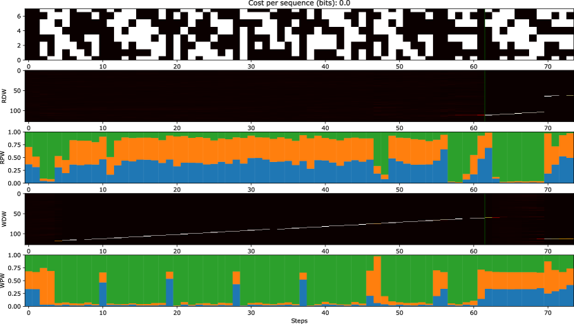
Figure 14: Copy+Associative Recall (p=3).

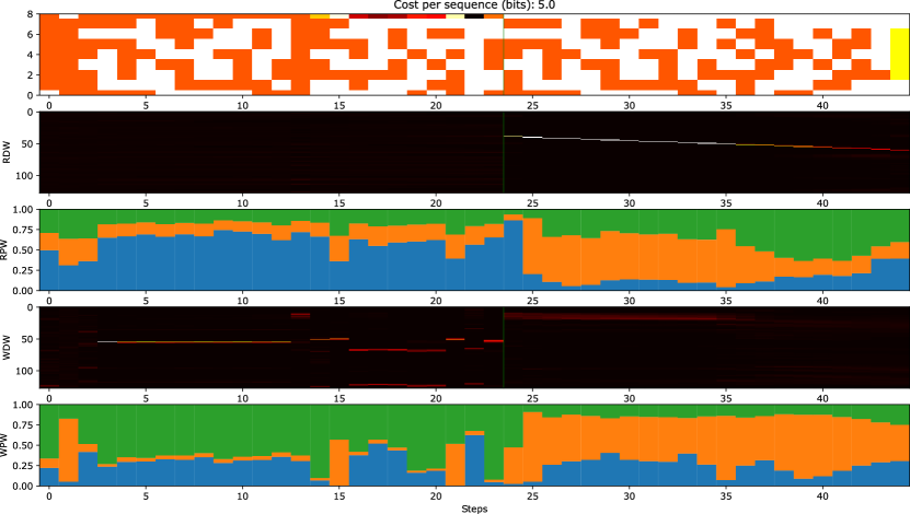
Figure 15: Copy+Priority Sort (p=3).

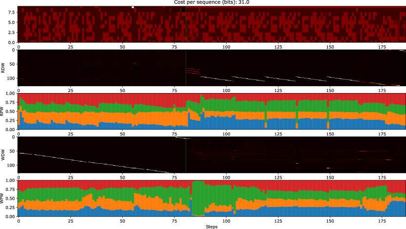
Figure 16: Copy+Repeat Copy+Associative Recall+Priority Sort (p=4).

B.3 Perseveration phenomenon in NTM (sequencing tasks)

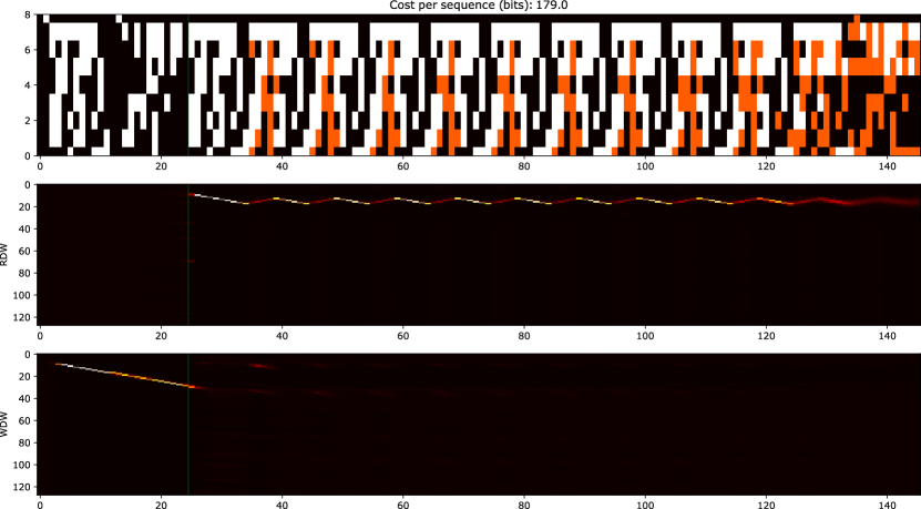
Figure 17: Copy+Repeat Copy perseveration (only Repeat Copy).

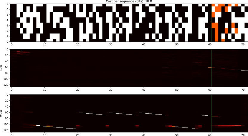
Figure 18: Copy+Associative Recall perseveration (only Copy).

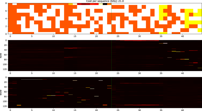
Figure 19: Copy+Priority Sort perseveration (only Copy).

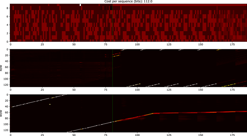
Figure 20: Copy+Repeat Copy+Associative Recall+Priority Sort perseveration (only Repeat Copy).

C Details on Synthetic Tasks

C.1 NTM single tasks

Tasks	#Read/Write Head		Controller Size		Memory Size		#Parameters
	NTM	NUTM	NTM	NUTM	NTM	NUTM	NTM	NUTM
Copy	1	1	100	80	128	128	63,260	52,206
Repeat Copy	1	1	100	80	128	128	63,381	52,307
Associative Recall	1	1	100	80	128	128	62,218	51,364
Dynamic N-grams	1	1	100	80	128	128	58,813	48,619
Priority Sort	5	5	200	150	128	128	344,068	302,398
Long Copy	1	1	100	80	256	256	63,260	52,206

Table 4: Model hyper-parameters (single tasks).

Tasks	Training	Testing
Copy	Sequence length range: [1, 20]	Sequence length: 120
Repeat Copy	Sequence length range: [1, 10]	Sequence length range: [10, 20]
	#Repeat range: [1, 10]	#Repeat range: [10, 20]
Associative Recall	#Item range: [2, 6]	#Item range: [6, 20]
	Item length: 3	Item length: 3
Dynamic N-grams	Sequence length: 50	Sequence length: 200
Priority Sort	#Item: 20	#Item: 20
	#Sorted Item: 16	#Sorted Item: 20
Long Copy	Sequence length range: [1, 40]	Sequence length: 200

Table 5: Task settings (single tasks).

C.2 NTM sequencing tasks

Tasks	#Read/Write Head		Controller Size		Memory Size		#Parameters
	NTM	NUTM	NTM	NUTM	NTM	NUTM	NTM	NUTM
C+RC	1	1	200	150	128	128	206,481	153,941
C+AR	1	1	200	150	128	128	206,260	153,770
C+PS	3	3	200	150	128	128	275,564	263,894
C+RC+AR+PS	3	3	250	200	128	128	394,575	448,379

Table 6: Model hyper-parameters (sequencing tasks).

Tasks	Training	Testing
C+RC	Sequence length range: [1, 10]	Sequence length range: [10, 20]
	#Repeat range: [1, 10]	#Repeat range: [10, 15]
C+AR	Sequence length range: [1, 10]	Sequence length range: [10, 20]
	#Item range: [2, 4]	#Item range: [4, 6]
	Item length: 8	Item length: 8
C+PS	Sequence length range: [1, 10]	Sequence length range: [10, 20]
	#Item: 10	#Item: 10
	#Sorted Item: 8	#Sorted Item: 10
C+RC+AR+PS	Sequence length range: [1, 10]	Sequence length range: [10, 20]
	#Repeat range: [1, 5]	#Repeat: 6
	#Item range: [2, 4]	#Item: 5
	Item length: 6	Item length: 6
	#Item: 10	#Item: 10
	#Sorted Item: 8	#Sorted Item: 10

Table 7: Task settings (sequencing tasks).

C.3 Continual procedure learning tasks

#Read/Write Head		Controller Size		Memory Size		#Parameters
NTM	NUTM	NTM	NUTM	NTM	NUTM	NTM	NUTM
1	1	200	150	128	128	206,444	196,590

Table 8: Model hyper-parameters (continual procedure learning tasks). NUTM uses 6 programs per head.

Tasks	Training	Testing
Copy	Sequence length range: [1, 10]	Sequence length range: [1, 10]
Repeat Copy	Sequence length range: [1, 5]	Sequence length range: [1, 5]
	#Repeat range: [1, 5]	#Repeat range: [1, 5]
Associative Recall	Sequence length: 3	Sequence length: 3
	#Item range: [2, 3]	#Item range: [2, 3]
	Item length: 3	Item length: 3
Priority Sort	#Item: 10	#Item: 10
	#Sorted Item: 8	#Sorted Item: 8

Table 9: Task settings (continual procedure learning tasks).

D Details on Few-shot Learning Task

We use similar hyper-parameters as in Santoro et al. (2016) , which are reported in Tab. 10.

Model	$p$	#Read Head	#Write Head	Controller Size	$N$	$M$	$\mathbf{M}_{p}.K$ Size
MANN (LRUA)	1	4	1	200	128	40	0
NUTM (LRUA)	2	4	1	180	128	40	2
NUTM (LRUA)	3	4	1	150	128	40	3

Table 10: Hyper-parameters for few-shot learning. All models use RMSprop optimizer with learning rate $10^{-4}$.

Testing accuracy through time is listed below,

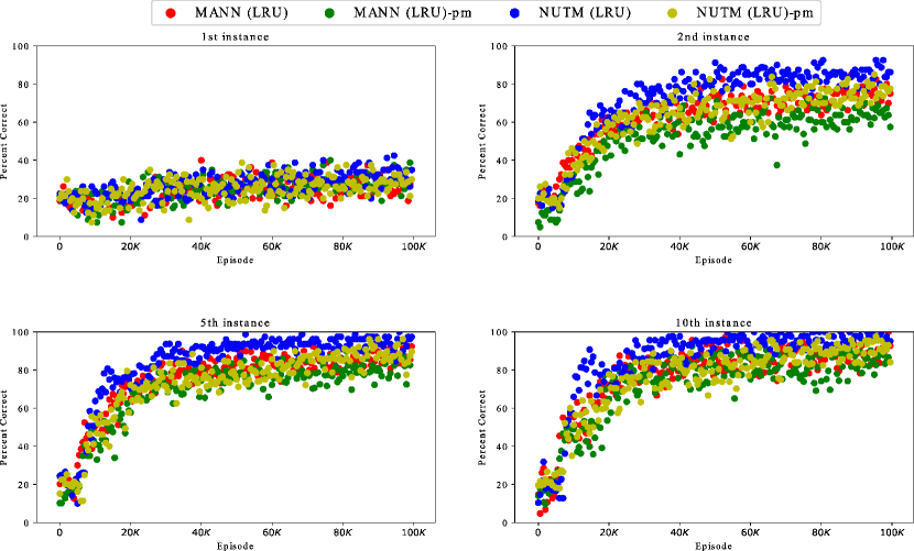
Figure 21: Testing accuracy during training (five random classes/episode, one-hot vector labels, of length 50).

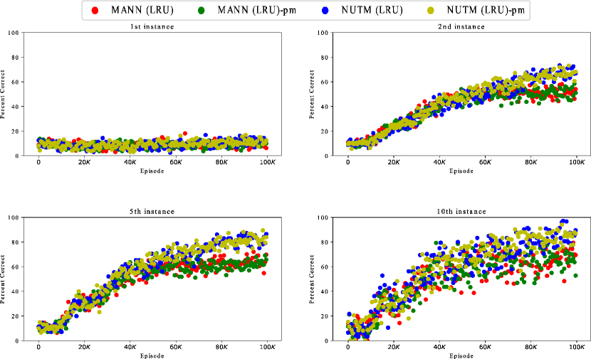
Figure 22: Testing accuracy during training (ten random classes/episode, one-hot vector labels, of length 75).

Model	Persistent	5 classes			10 classes
	memory	$2^{nd}$	$3^{rd}$	$5^{th}$	$2^{nd}$	$3^{rd}$	$5^{th}$
MANN (LRUA)*	No	82.8	91.0	94.9	-	-	-
MANN (LRUA)	No	82.3	88.7	92.3	52.7	60.6	64.7
NUTM (LRUA)	No	85.7	91.3	95.5	68.0	78.1	82.8
Human*	Yes	57.3	70.1	81.4	-	-	-
MANN (LRUA)*	Yes	$\approx 58.0$	-	$\approx 75.0$	$\approx 60.0$	-	$\approx 80.0$
MANN (LRUA)	Yes	66.2	73.4	81.0	51.3	59.2	63.3
NUTM (LRUA)	Yes	77.8	85.8	89.8	69.0	77.9	82.7

Table 11: Test-set classification accuracy (%) on the Omniglot dataset after 100,000 episodes of training. * denotes available results from Santoro et al. (2016) (some are estimated from plotted figures).

E Details on bAbI Task

We train the models using RMSprop optimizer with fixed learning rate of $10^{-4}$ and momentum of 0.9. The batch size is 32 and we adopt layer normalization Lei Ba et al. (2016) to DNC’s layers. Following Franke et al. (2018) practice, we also remove temporal linkage for faster training. The details of hyper-parameters are listed in Table 12. Full NUTM ($p=4$) results are reported in Table 13.

#Read Head	#Write Head	Controller Size	$N$	$M$	$p$	$\mathbf{M}_{p}.K$ Size	#Parameters
4	1	256	196	64	1	1	891,136
4	1	200	196	64	2	2	934,787
4	1	172	196	64	4	4	794,773

Table 12: NUTM hyper-parameters for bAbI.

Task	bAbI Best Results	bAbI Mean Results
1: 1 supporting fact	0.0	0.0 $\pm$ 0.0
2: 2 supporting facts	0.2	0.6 $\pm$ 0.3
3: 3 supporting facts	4.0	7.6 $\pm$ 3.9
4: 2 argument relations	0.0	0.0 $\pm$ 0.0
5: 3 argument relations	0.4	1.0 $\pm$ 0.4
6: yes/no questions	0.0	0.0 $\pm$ 0.0
7: counting	1.9	1.5 $\pm$ 0.8
8: lists/sets	0.6	0.3 $\pm$ 0.2
9: simple negation	0.0	0.0 $\pm$ 0.0
10: indefinite knowledge	0.1	0.1 $\pm$ 0.0
11: basic coreference	0.0	0.0 $\pm$ 0.0
12: conjunction	0.0	0.0 $\pm$ 0.0
13: compound coreference	0.1	0.0 $\pm$ 0.0
14: time reasoning	0.3	1.6 $\pm$ 2.2
15: basic deduction	0.0	2.6 $\pm$ 8.3
16: basic induction	49.3	52.0 $\pm$ 1.7
17: positional reasoning	4.7	18.4 $\pm$ 12.7
18: size reasoning	0.4	1.6 $\pm$ 1.1
19: path finding	4.3	23.7 $\pm$ 32.2
20: agent’s motivation	0.0	0.0 $\pm$ 0.0
Mean Error (%)	3.3	5.6 $\pm$ 1.9
Failed (Err. >5%)	1	3 $\pm$ 1.2

Table 13: NUTM ($p=4$) bAbI best and mean errors (%).

F Example of memory operation function in NTM

In NTM, $\xi_{t}=\left\{\beta_{t},k_{t},g_{t},s_{t},e_{t},v_{t}\right\}$. The memory addressing weight is initially computed by content-based attention,

$$w_{t}^{c}\left(i\right)=\frac{\exp\left(\beta_{t}m\left(k_{t},M_{t}\left(i\right)\right)\right)}{\stackrel{{\scriptstyle[}}{{j}}=1]{D}{\sum}\exp\left(\beta_{t}m\left(k_{t},M_{t}\left(j\right)\right)\right)}$$ (8)

Here, $w_{t}^{c}\in\mathbb{R}^{N}$ is the content-based weight, $\beta_{t}$ is a strength scalar, and $m$ is implemented as cosine similarity

$$m\left(k_{t},M_{t}(i)\right)=\frac{k_{t}\cdot M_{t}(i)}{||k_{t}||\cdot||M_{t}(i)||}$$ (9)

In addition, NTM supports location-based addressing started with an interpolation between content-based weight and the previous weight

$$w_{t}^{g}=g_{t}w_{t}^{c}+\left(1-g_{t}\right)w_{t}$$ (10)

where $g_{t}$ is the interpolation gate that determines to use (or ignore) content-based addressing. Then, NTM can shift the address to other rows by performing convolution shift modulo $R$,

$$\tilde{w_{t}}\left(i\right)=\stackrel{{\scriptstyle[}}{{j}}=0]{R}{\sum}w_{t}^{g}\left(i\right)s_{t}\left(i-j\right)$$ (11)

where $s_{t}$ is the shift weighting. To prevent the shifted weight from blurring, sharpening is applied

$$w_{t}\left(i\right)=\frac{\tilde{w_{t}}\left(i\right)^{\gamma}}{\underset{j}{\sum}\tilde{w_{t}}\left(j\right)^{\gamma}}$$ (12)

Then, the memory is updated as follows,

$$M_{t}^{erased}\left(i\right) =M_{t-1}\left(i\right)\left[1-w_{t}\left(i\right)e_{t}\right]$$ (13)

$$M_{t}\left(i\right) =M_{t}^{erased}\left(i\right)+w_{t}\left(i\right)v_{t}$$ (14)

where $e_{t}\in\mathbb{R}^{D}$ and $v_{t}\in\mathbb{R}^{D}$ are erase vector and update vector, respectively. The read value is computed using the same address weight as follows,

$$r=\stackrel{{\scriptstyle[}}{{i}}=1]{N}{\sum}w_{t}\left(i\right)M_{t}\left(i\right)$$ (15)

G Others

If we deliberately set the key dimension equal to the number of programs, we can even place an orthogonal basis constraint on the key space of NSM by minimizing the following loss,

$$l_{p_{2}}=\left\|\mathbf{M}_{p}.K\mathbf{M}_{p}.K^{T}-\mathbf{I}\right\|$$ (16)

where $\mathbf{M}_{p}.K$ and $\mathbf{I}$ denote the key part in NSM and the identity matrix, respectively.

Direct attention is one special case of key-value attention when the memory keys form orthogonal basis. When this happens, the generated key $k_{t}^{p}$ plays a direct role as the attention weight $w_{t}^{p}$. Thus, using key-value attention is more generic.

For all tasks, $\eta_{t}$ is fixed to $0.1$, reducing with decay rate of $0.9$.

Ablation study’s learning losses with mean and error bar are plotted in Fig. 23.

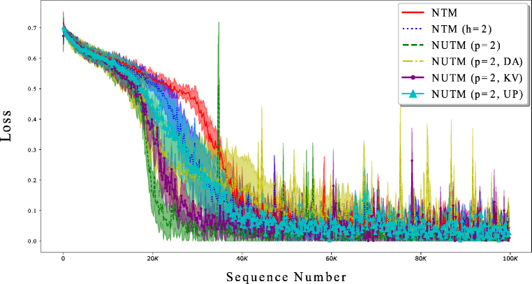
Figure 23: Learning curves on Associative Recall (AR) ablation study.

References

- Andreas et al. (2016a) Jacob Andreas, Marcus Rohrbach, Trevor Darrell, and Dan Klein. Learning to compose neural networks for question answering. In Proceedings of the 2016 Conference of the North American Chapter of the Association for Computational Linguistics: Human Language Technologies, pp. 1545–1554, 2016a. doi: 10.18653/v1/N16-1181. URL https://www.aclweb.org/anthology/N16-1181.
- Andreas et al. (2016b) Jacob Andreas, Marcus Rohrbach, Trevor Darrell, and Dan Klein. Neural module networks. In Proceedings of the IEEE Conference on Computer Vision and Pattern Recognition, pp. 39–48, 2016b.
- Andrew Gelman (2006) Jennifer Hill Andrew Gelman. Data Analysis Using Regression and Multilevel/Hierarchical Models. Cambridge University Press, 2006.
- Ba et al. (2016) Jimmy Ba, Geoffrey E Hinton, Volodymyr Mnih, Joel Z Leibo, and Catalin Ionescu. Using fast weights to attend to the recent past. In Advances in Neural Information Processing Systems, pp. 4331–4339, 2016.
- Blumenfeld (2010) Hal Blumenfeld. Neuroanatomy through Clinical Cases. Oxford University Press, 2010.
- Broesch (2009) James D. Broesch. Chapter 8 - digital signal processors. In James D. Broesch (ed.), Digital Signal Processing, Instant Access, pp. 135 – 146. Newnes, Burlington, 2009. ISBN 978-0-7506-8976-2. doi: https://doi.org/10.1016/B978-0-7506-8976-2.00008-0. URL http://www.sciencedirect.com/science/article/pii/B9780750689762000080.
- Casey (1996) Mike Casey. The dynamics of discrete-time computation, with application to recurrent neural networks and finite state machine extraction. Neural computation, 8(6):1135–1178, 1996.
- Cohen et al. (2014) Patricia Cohen, Stephen G West, and Leona S Aiken. Applied multiple regression/correlation analysis for the behavioral sciences. Psychology Press, 2014.
- Csordas & Schmidhuber (2019) Robert Csordas and Juergen Schmidhuber. Improving differentiable neural computers through memory masking, de-allocation, and link distribution sharpness control. In International Conference on Learning Representations, 2019. URL https://openreview.net/forum?id=HyGEM3C9KQ.
- Franke et al. (2018) Jörg Franke, Jan Niehues, and Alex Waibel. Robust and scalable differentiable neural computer for question answering. In Proceedings of the Workshop on Machine Reading for Question Answering, pp. 47–59. Association for Computational Linguistics, 2018. URL http://aclweb.org/anthology/W18-2606.
- French (1999) Robert M French. Catastrophic forgetting in connectionist networks. Trends in cognitive sciences, 3(4):128–135, 1999.
- Graves et al. (2014) Alex Graves, Greg Wayne, and Ivo Danihelka. Neural turing machines. arXiv preprint arXiv:1410.5401, 2014.
- Graves et al. (2016) Alex Graves, Greg Wayne, Malcolm Reynolds, Tim Harley, Ivo Danihelka, Agnieszka Grabska-Barwińska, Sergio Gómez Colmenarejo, Edward Grefenstette, Tiago Ramalho, John Agapiou, et al. Hybrid computing using a neural network with dynamic external memory. Nature, 538(7626):471–476, 2016.
- Ha et al. (2016) David Ha, Andrew Dai, and Quoc V Le. Hypernetworks. arXiv preprint arXiv:1609.09106, 2016.
- Hinton & Plaut (1987) Geoffrey E Hinton and David C Plaut. Using fast weights to deblur old memories. In Proceedings of the ninth annual conference of the Cognitive Science Society, pp. 177–186, 1987.
- Huang (2018) Francis L Huang. Multilevel modeling and ordinary least squares regression: how comparable are they? The Journal of Experimental Education, 86(2):265–281, 2018.
- Jang et al. (2016) Eric Jang, Shixiang Gu, and Ben Poole. Categorical reparameterization with gumbel-softmax. arXiv preprint arXiv:1611.01144, 2016.
- Le et al. (2018a) Hung Le, Truyen Tran, Thin Nguyen, and Svetha Venkatesh. Variational memory encoder-decoder. In Advances in Neural Information Processing Systems, pp. 1515–1525, 2018a.
- Le et al. (2018b) Hung Le, Truyen Tran, and Svetha Venkatesh. Dual memory neural computer for asynchronous two-view sequential learning. In Proceedings of the 24th ACM SIGKDD International Conference on Knowledge Discovery; Data Mining, KDD ’18, pp. 1637–1645, New York, NY, USA, 2018b. ACM. ISBN 978-1-4503-5552-0. doi: 10.1145/3219819.3219981. URL http://doi.acm.org/10.1145/3219819.3219981.
- Le et al. (2019) Hung Le, Truyen Tran, and Svetha Venkatesh. Learning to remember more with less memorization. In International Conference on Learning Representations, 2019. URL https://openreview.net/forum?id=r1xlvi0qYm.
- Lei Ba et al. (2016) Jimmy Lei Ba, Jamie Ryan Kiros, and Geoffrey E Hinton. Layer normalization. arXiv preprint arXiv:1607.06450, 2016.
- Mozer & Das (1993) Michael C Mozer and Sreerupa Das. A connectionist symbol manipulator that discovers the structure of context-free languages. In Advances in neural information processing systems, pp. 863–870, 1993.
- Rae et al. (2016) Jack Rae, Jonathan J Hunt, Ivo Danihelka, Timothy Harley, Andrew W Senior, Gregory Wayne, Alex Graves, and Tim Lillicrap. Scaling memory-augmented neural networks with sparse reads and writes. In Advances in Neural Information Processing Systems, pp. 3621–3629, 2016.
- Santoro et al. (2016) Adam Santoro, Sergey Bartunov, Matthew Botvinick, Daan Wierstra, and Timothy Lillicrap. Meta-learning with memory-augmented neural networks. In International conference on machine learning, pp. 1842–1850, 2016.
- Schlag & Schmidhuber (2017) Imanol Schlag and Jürgen Schmidhuber. Gated fast weights for on-the-fly neural program generation. In NIPS Metalearning Workshop, 2017.
- Schmidhuber (1993a) J Schmidhuber. Reducing the ratio between learning complexity and number of time varying variables in fully recurrent nets. In International Conference on Artificial Neural Networks, pp. 460–463. Springer, 1993a.
- Schmidhuber (1993b) Jürgen Schmidhuber. A self-referential weight matrix. In International Conference on Artificial Neural Networks, pp. 446–450. Springer, 1993b.
- Siegelmann & Sontag (1995) Hava T Siegelmann and Eduardo D Sontag. On the computational power of neural nets. Journal of computer and system sciences, 50(1):132–150, 1995.
- Sukhbaatar et al. (2015) Sainbayar Sukhbaatar, arthur szlam, Jason Weston, and Rob Fergus. End-to-end memory networks. In C. Cortes, N. D. Lawrence, D. D. Lee, M. Sugiyama, and R. Garnett (eds.), Advances in Neural Information Processing Systems, pp. 2440–2448. 2015. URL http://papers.nips.cc/paper/5846-end-to-end-memory-networks.pdf.
- Sutskever et al. (2011) Ilya Sutskever, James Martens, and Geoffrey E Hinton. Generating text with recurrent neural networks. In Proceedings of the 28th International Conference on Machine Learning (ICML-11), pp. 1017–1024, 2011.
- Thrun (1998) Sebastian Thrun. Lifelong learning algorithms. In Learning to learn, pp. 181–209. Springer, 1998.
- Tiňo et al. (1998) Peter Tiňo, Bill G Horne, C Lee Giles, and Pete C Collingwood. Finite state machines and recurrent neural networks–automata and dynamical systems approaches. In Neural networks and pattern recognition, pp. 171–219. Elsevier, 1998.
- Turing (1936) A.M Turing. On computable numbers, with an application to the entscheidungsproblem. In Proceedings of the London Mathematical Society, 1936.
- von der Malsburg (1981) Christoph von der Malsburg. The correlation theory of brain function, 1981. URL http://cogprints.org/1380/.
- von Neumann (1993) John von Neumann. First draft of a report on the edvac. IEEE Ann. Hist. Comput., 15(4):27–75, October 1993. ISSN 1058-6180. doi: 10.1109/85.238389. URL https://doi.org/10.1109/85.238389.
- Weston et al. (2015) Jason Weston, Antoine Bordes, Sumit Chopra, Alexander M Rush, Bart van Merriënboer, Armand Joulin, and Tomas Mikolov. Towards ai-complete question answering: A set of prerequisite toy tasks. arXiv preprint arXiv:1502.05698, 2015.
- Zenke et al. (2017) Friedemann Zenke, Ben Poole, and Surya Ganguli. Continual learning through synaptic intelligence. In Proceedings of the 34th International Conference on Machine Learning-Volume 70, pp. 3987–3995. JMLR. org, 2017.