A new, rotating hot corino in Serpens

Abstract

We have observed 29 transitions corresponding to 12 distinct species and 7 additional isotopologs toward the deeply embedded Class 0 young stellar object Ser-emb 1 with the Atacama Large Millimeter Array at $\sim$ 1 mm. The detected species include CH₃OH and two complex organic molecules, CH₃OCH₃ and CH₃OCHO. The emission of CH₃OH and the two COMs is compact, and the CH₃OH rotational temperature is 261 $\pm$ 46 K, implying that Ser-emb 1 hosts a hot corino. The derived CH₃OH, CH₃OCH₃ and CH₃OCHO column densities are at least (1.2 $\pm$ 0.4) $\times$ 10¹⁷ cm^-2, (9.2 $\pm$ 3.8) $\times$ 10¹⁶ cm^-2, and (9.1 $\pm$ 3.6) $\times$ 10¹⁶ cm^-2, respectively, comparable to the values found for other Class 0 hot corinos. In addition, we observe evidence of rotation at compact scales: two of the more strongly detected lines, corresponding to C¹⁸O and H₂CO present spatially resolved red- and blue-shifted compact emission orthogonal to the direction of a jet and outflow traced by CO, SiO, and several other molecules. The spatial coincidence of the hot corino emission and a possible disk in a compact region around the central protostar suggests that these structures may be physically and/or chemically related.

1 Introduction

In the early stages of star formation (i.e., Class 0/I sources, see, e.g., André et al., 1993; Robitaille et al., 2006) the central protostar is embedded in a dense envelope as the parental dense core gravitationally collapses. This cold dense envelope warms up close to the central protostar and, where the temperature is high enough, the ice mantles on the surfaces of dust grains sublimate. This leads to the formation of a chemically-rich hot core (around high-mass protostars) or hot corino (around low-mass protostars), although not all observed warm compact cores present a hot core/corino chemistry (see Herbst & van Dishoeck, 2009, and references therein). Hot cores and hot corinos are characterized by the presence of saturated, complex (6+ atoms) organic molecules (COMs) with abundances up to 10^-7 with respect to H₂, and rotational temperatures above 100 K (i.e., the water ice sublimation temperature). The typical size of hot corinos is about 100 au or less, with temperatures of around 100 K, while hot cores are warmer (T $\sim$300 K) and much larger (up to 10000 au, Herbst & van Dishoeck, 2009). Hot corinos are harder to detect than their more massive analogs, due to their lower envelope masses and luminosities leading to weaker lines, and only nine hot corinos have been detected to date: IRAS 16293-2422 (Cazaux et al., 2003), IRAS 4A (Bottinelli et al., 2004), IRAS 2 (Jørgensen et al., 2005), IRAS 4B (Bottinelli et al., 2007), HH 212 (Codella et al., 2016), B335 (Imai et al., 2016), L483 (Oya et al., 2017), B1b (Lefloch et al., 2018), and SVS13-A (the only Class I hot corino, Bianchi et al., 2019).

COM observations are not limited to hot cores and hot corinos. Marcelino et al. (2007) reported the detection of methanol and acetaldehyde in the cold prestellar core TMC-1, with abundances up to only a few $\times$ 10^-9; and more recently, COMs have been also observed in the prestellar core L1544 (Vastel et al., 2014; Jiménez-Serra et al., 2016). In star-forming regions, COMs have been also detected in outflows (Arce et al., 2008; Codella et al., 2017; Lefloch et al., 2018); and in the lukewarm and cold envelope around the B1b protostar (Öberg et al., 2010). These observations are consistent with a three-phases COM-formation scenario (see, e.g., Herbst & van Dishoeck, 2009). Roughly, during the cold phase of star formation (T $\sim$ 10 K, prior and during the isothermal collapse of the cold prestellar core), organics such as H₂CO and CH₃OH are mainly formed in the ice mantles on top of dust grains. The energetic processing of the ice mantles produce radicals such as HCO^. and CH₃O^. that are able to diffuse at lukewarm temperatures (T $>$ 20 K, once the protostar warms up the surrounding envelope) and react to form first-generation COMs like CH₃OCH₃ or CH₃OCHO (Garrod et al., 2006, 2008), while further gas-phase reactions lead to the formation of the second generation of COMs during the hot core/corino phase.

During the Class 0/I stages of star formation where hot corinos are detected, protostellar disks begin to form around the low-mass protostars due to conservation of angular momentum of the infalling-rotating envelope. Observations seem to show an evolutionary trend in protostellar disks (Yen et al., 2013) from slow pseudodisks (a flattened envelope), to Keplerian disks (disks rotating fast enough to become centrifugally supported). These disks further evolve to the protoplanetary disks observed around Class II/III T Tauri and Herbig Ae/Be protostars. Protostellar disks, and especially their chemistry, are harder to observe than the more evolved protoplanetary disks, mainly because of the difficulties in separating the emission from the disk and from the dense envelope in which it is embedded. Only a handful of protostellar disks have been confirmed toward Class 0 sources (namely, IRAS 4A2, L1527, VLA 1623A, L1448-mm, HH 212, IRS 7B, and Lupus 3MMS, see Choi et al., 2010; Tobin et al., 2012b; Murillo et al., 2013; Yen et al., 2013; Codella et al., 2014; Lindberg et al., 2014; Yen et al., 2017), with sizes around 50$-$150 au, similar to the typical size of a hot corino.

Previous works have tried to connect the presence of a hot corino with disk formation in Class 0/I sources. Jørgensen et al. (2005) had suggested a protostellar disk as a more dynamically stable location for the complex molecules in the IRAS 2A hot corino than the infalling envelope. Indeed, two of the nine detected sources with hot corinos (IRAS 4A2 and HH 212) show strong evidences of a protostellar disk, while the presence of such structure in a third hot corino source (IRAS 16293A) is also plausible. In IRAS 4A2, the NH₃ emission distribution from red- to blue-shifted velocities in the direction perpendicular to the bipolar jet was interpreted as a protostellar disk upon the fitting of the position-velocity (PV) diagram to a model of a disk with Keplerian rotation (Choi et al., 2010). A similar signature consistent with Keplerian rotation was found for the C¹⁷O line emission in HH 212 (Codella et al., 2014). More recently, Lee et al. (2017); Codella et al. (2018); Lee et al. (2019) have observed emission from a total of 9 COMs above and below the edge-on dusty disk traced by the continuum emission in HH 212, indicating that the hot corino in this source is actually a warm atmosphere of the disk. In other sources, though, the connection between hot corino emission and the protostellar disk is more tenuous. Oya et al. (2016) and Oya et al. (2017) have studied the kinematic structure of two other sources presenting hot corino chemistry: IRAS 16293-2422 and L483, respectively. They use a three-dimensional ballistic model (Oya et al., 2014) considering two physical components (a flattened infalling-rotating envelope and a Keplerian disk, separated by a centrifugal barrier) to simulate the emission of different molecular lines and reproduce their PV diagrams. In IRAS 16293A, they find that CH₃OH and CH₃OCHO are present in a ring-like structure around the centrifugal barrier with an inner radius of $\sim$55 au, interpreted as the evaporation from dust grains due to the accretion shocks expected in that region (Oya et al., 2016). Modelling of L483 in Oya et al. (2017) also indicates that the most likely location of the two detected COMs (NH₂CHO and CH₃OCHO) is the Keplerian disk formed within the centrifugal barrier. However, Jacobsen et al. (2019) ruled out the presence of a Keplerian disk in L483 down to at least 15 au, using higher spatial resolution observations, and concluded that the hot corino chemistry in this source is taking place at larger scales in the infalling-rotating envelope.

In this work, we explore the connection between hot corino emission and rotation in the Class 0 source Ser-emb 1. The Serpens molecular cloud is a star-forming cloud harboring 34 embedded protostars (9 Class 0 sources and 25 Class I sources, Enoch et al., 2009), located at a distance of $d$ = 436 $\pm$ 9 pc (Ortiz-León et al., 2018). Enoch et al. (2011) reported evidences for a compact disk component around seven of them (Ser-emb 1, Ser-emb 4, Ser-emb 6, Ser-emb 7, Ser-emb 8, Ser-emb 11, Ser-emb 15, and Ser-emb 17) based on the continuum emission detected at long uv baselines (and therefore coming from dust in compact regions around the central object). Among these seven sources, Ser-emb 1 is located in the Serpens Cluster B, and it is the least evolved protostar in the cloud according to its bolometric temperature (39 K). Its remaining envelope mass is 3.1 $M_{\odot}$, and the estimated disk mass is 0.28 $M_{\odot}$ (Enoch et al., 2011). However, spatially and spectrally resolved line observations are needed to confirm the presence of a rotationally supported disk.

We present ALMA Band 6 observations of Ser-emb 1 aimed at the study of the structure of the source, and the evaluation of its chemical richness. The paper is organized as follows: ALMA observations, calibration, and imaging strategies are described in Sect. 2. An overview of the different structural components observed in Ser-emb 1 is presented in Sect. 3.1. The molecular detections are presented in Sect. 3.2; and the evidences for a hot corino and a possible protostellar disk are shown in Sections 3.3 and 3.4, respectively, and discussed in Sect. 4. Section 5 presents the final conclusions.

2 Observations

The Ser-emb 1 observations analyzed in this paper were obtained within a larger ALMA project (#2015.1.00964.S) on chemistry in disks at different evolutionary stages. The observations were centered at $RA_{\rm J2000}$ = 18h 29min 09.09s, $DEC_{\rm J2000}$ = +00^∘ 31^′ 30.90^′′, and completed during Cycle 3 using two different Band 6 frequency settings. The first frequency setting consisted on eight spectral windows placed between 217 GHz and 233 GHz. Seven spectral windows have bandwidths of 58.6 or 117.2 MHz, and a spectral resolution of $\sim$0.16 km s^-1. The eighth spectral window has a bandwidth of 1.875 GHz, and a lower spectral resolution of $\sim$0.63 km s^-1. This frequency setting was observed on June 05 and 14, 2016, using 42 antennas (longest baseline of 772.8 m) for a total on source time of 19.2 min. The second frequency setting included seven spectral windows placed between 243 GHz and 262 GHz. Six spectral windows have a bandwidth of 117.2 MHz, and a spectral resolution of $\sim$0.14 km s^-1. The seventh spectral window has a bandwidth of 1.875 GHz, and a spectral resolution of $\sim$0.60 km s^-1. The observations of this frequency setting were carried out on May 15 and 16, 2016, using 41 antennas (longest baseline of 640.0 m) for a total on source time of 22.5 min. The observed spectral windows are listed in the Appendix.

2.1 Calibration

The observed visibilities were initially calibrated by ALMA staff with the Common Astronomy Software Applications (CASA) versions 4.5.3 and 4.7.0, using the sources J1751+0939, J1830+0619 as bandpass and phase calibrators, respectively, and Titan as the absolute flux calibrator. The continuum data of each spectral window (channel-averaged visibilities after flagging line emission channels) was further self-calibrated in 1-2 rounds, and the solutions were applied to the native resolution visibilities. The continuum was substracted from the self-calibrated visibilities in the $uv$ plane using line-free channels.

2.2 Generation of the source spectrum

Imaging of the self-calibrated, continuum-substracted data cubes at their native spectral resolution was performed with the CASA version 5.3.0 using the task TCLEAN with Brigss weighting of the baselines. During the imaging process, an auto-mask was applied independently to every channel of the self-calibrated data cubes, using the parameters sidelobethreshold = 2.5 $\times$ rms, noisethreshold = 3.0 $\times$ rms, minbeamfrac = 0.3, cutthreshold = 0.4, lownoisethreshold = 1.5 $\times$ rms, and growiterations = 75. For confirmation purposes, we imaged the C¹⁸O 2 $-$ 1 line manually masking every channel, and obtained the same result.

The robustness parameter was set to 0.5 for the Briggs weighting of the baselines during this first round of imaging. The rms per channel (averaged over ten line-free channels) is 5$-$9 mJy beam^-1 in the high-spectral resolution windows, and $\sim$2 mJy beam^-1 in the low-spectral resolution windows. The average synthesized beam was 0.57$\arcsec$ $\times$ 0.47$\arcsec$. The particular values for each spectral window can be found in Sect. A, where the exact frequency range covered and spectral resolution for each spectral window is also listed. The spectrum of the source at the central pixel, which corresponds to the position of the continuum peak, was then extracted from the FITS file generated by CASA for every cleaned data cube, and subsequently used to detect and identify molecular transitions (see Sect. 3.2 and Fig. 2).

2.3 Imaging of the individual lines

The identified transitions in the extracted spectrum (see Fig. 2 and Table 1) were individually re-imaged following the same process explained above, but using a robustness parameter of 0.0 to improve the angular resolution. The averaged rms of the image cubes per channel increased to 6 $-$ 12 mJy beam^-1 ($\sim$3 mJy beam^-1 for the low-resolution spectral window), while the average size of the synthesized beam decreased to $\sim$ 0.50$\arcsec$ $\times$ 0.42$\arcsec$ (values for each spectral window can be found in Table 4), which translates to a beam radius of $\sim$100 au at a distance of 436 pc. Two of the targeted lines, N₂D⁺ 3 $-$ 2 and C₂H 3 $-$ 2, were not observed in the extracted spectrum, but extended emission is present. These lines were imaged with a robustness parameter of 0.5 to enhance the signal-to-noise ratio. All images were corrected for the primary beam.

3 Results

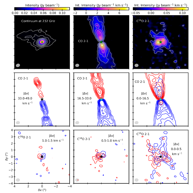
Figure 1: The top left panel shows the continuum map centered at 232 GHz along with the 3, 6, 12, 18, 24, 48, and 96$\sigma$ contours ($\sigma$ = 0.3 mJy beam^-1). The position of the continuum peak is indicated with a star in every panel. The middle and right top panels show the moment 0 maps along with the 3, 6, 9, 12, 15, 18, 24, and 30$\sigma$ contours for the CO and C¹⁸O 2 $-$ 1 transitions, respectively (maps are clipped at 1$\sigma$). The moment 0 rms is indicated in Table 1. The blue- and red-shifted moment 0 maps, split into three different velocity components are shown in the middle and bottom rows (only contours). The velocity range of every velocity component is indicated in every panel, and the size of the synthesized beam ($\sim$ 0.50$\arcsec$ $\times$ 0.42$\arcsec$) is also shown in the lower left of every panel (see also Sect. A)

3.1 Overview of the source

Figure 1 presents an overview of the Ser-emb 1 source structure, as traced by millimeter dust continuum emission, and CO 2 $-$ 1 and C¹⁸O 2 $-$ 1 line emission. The continuum map shown in the upper left panel was generated by combining all line-free channels in the wide-band spectral window centered at $\sim$232 GHz. The continuum peak is assumed to correspond to the position of the central protostar, and is marked in the remaining panels.

The integrated moment 0 map over the full line width of the CO 2 $-$ 1 emission is shown in the upper middle panel of Fig. 1, and traces a bipolar outflow in the north-east to south-west direction (NE$-$SW, position angle of PA = 12.2^∘) driven by the central protostar. The integrated blue- and red-shifted emission with respect to the systemic velocity of the source ($V_{LSR}$ $\sim$ 8.5 km s^-1) is represented in the middle row panels of Fig. 1, decomposed into three velocity components. The high-velocity emission ($|\Delta$v$|$ $>$ 33 km s^-1 with respect to $V_{LSR}$ of the source, middle left panel) traces a collimated jet, while the low-velocity emission ($|\Delta$v$|$ $<$ 16 km s^-1, middle right panel) shows a wide-angle, v-shaped slower outflow.

The top right panel of Fig. 1 shows the integrated moment 0 map of the C¹⁸O 2 $-$ 1 emission, which is limited to the core of the source and the slower outflow region traced by the low-velocity CO 2 $-$ 1 emission. The three bottom panels present the integrated blue- and red-shifted C¹⁸O emission, also split into high- ($|\Delta$v$|$ $>$ 1.0 km s^-1), mid- (0.5 $<$ $|\Delta$v$|$ $<$ 1.0 km s^-1), and low-velocities ($|\Delta$v$|$ $<$ 0.5 km s^-1, from left to right, respectively) components. We note that these three velocity components are all included in the low-velocity map of the much broader CO emission. The low-velocity component (bottom right panel) presents emission detected above the 3$\sigma$ level up to $\sim$2 $\arcsec$ from the central protostar ($\sim$800 au). The blueshifted emission is brighter on the west side, while the redshifted emission is predominantly seen in the east side of the source. A similar distribution for the HCO⁺ 4 $-$ 3 low velocity ($|\Delta$v$|$ $<$ 1.5 km s^-1) emission in HH 212 was interpreted as a rotation contribution to the infall motion of the flattened envelope in Lee et al. (2017). The high-velocity component (bottom left panel) is detected in a compact region within $\sim$0.5$\arcsec$ ($\sim$200 au) of the central protostar, and is thus marginally resolved with a beam size of $\sim$ 0.53$\arcsec$ $\times$ 0.46$\arcsec$ (Table 4). Therefore, the actual radius of this compact component could be $<$200 au. The emission shows a gradient from red- to blue-shifted velocities in the direction perpendicular to the CO jet (PA = -77.7^∘), indicating that rotation may dominate the motion of this component (see, e.g., Lee et al., 2017). The rotation could not be checked for the CO 2 $-$ 1 transition because of self-absorption at low velocities close to the continuum peak.

3.2 Molecular detections

Figure 2: Spectrum of the Ser-emb 1 source toward the continuum peak after continuum substraction, re-binned to a spectral resolution of 0.5 MHz. Tentative assignments are indicated in red. Unassigned lines above 4$\sigma$ are marked with a U.

Table 1: Identified molecular transitions toward Ser-emb 1. Tentative assignments are indicated with a ^∗.

Molecule	Transition	Frequency	log(Aul)	$g_{up}$	$E_{up}$	$V_{LSR}$	FWHM	Mom. 0 Int.(a)	Mom. 0 rms(a)
		(GHz)	(s-1)		(K)	(km s-1)		(mJy beam-1 km s-1)
CO	2 $-$ 1	230.538	-6.16	5	16.60	$\cdots$ (b)	$\cdots$ (b)	7719.4	277.5(c)
13CO	2 $-$ 1	220.399	-6.22	5	15.87	$\cdots$ (b)	$\cdots$ (b)	110.8	9.8
C18O	2 $-$ 1	219.560	-6.22	5	15.81	8.71	2.13	118.6	6.1
CS	5 $-$ 4	244.936	-3.52	11	35.27	8.68	2.66	366.4	7.9
SiO	6 $-$ 5	260.518	-3.04	13	43.74	$\cdots$ (b)	$\cdots$ (b)	16069.6	276.2(c)
DCN	3 $-$ 2	217.238	-3.49	33	20.85	8.48	5.33(d)	71.3	9.3
H13CN	32 $-$ 22	259.012	-3.34	33	24.86	8.95	5.51(d)	317.7	7.5
HC15N	3 $-$ 2	258.157	-3.09	7	24.78	8.89	3.78	60.3	5.4
HCC13CN∗	27 $-$ 26	244.589	-2.94	165	164.34	8.25	2.95	31.2	6.8
HNO∗	30,3 $-$ 20,2	244.364	-4.37	38	23.46	9.01	1.49(d)	26.4	7.6
N2D+	3 $-$ 2	231.322	-2.67	63	22.20	$\cdots$ (b)	$\cdots$ (b)	29.1	7.0
C2H	3 $-$ 2	262.208	-5.24	7	25.16	$\cdots$ (b)	$\cdots$ (b)	17.1	4.4
SO2	113,9 $-$ 112,10	262.257	-3.85	23	82.80	8.98	3.05	173.8	7.4
SO2	140,14 $-$ 131,13	244.254	-3.79	29	93.90	8.90	3.77	294.6	6.8
OCS	20 $-$ 19	243.218	-4.38	41	122.57	8.41	3.00	168.7	8.7
O13CS	18 $-$ 17	218.199	-4.52	37	99.49	8.74	3.02	47.8	4.9
H2CS∗	71,6 $-$ 61,5	244.048	-3.68	45	60.05	8.41	3.37	37.7	7.6
H2CO	30,3 $-$ 20,2	218.222	-3.55	7	20.96	8.81	3.88	214.5	5.4
H2CO	32,2 $-$ 22,1	218.476	-3.80	7	68.09	8.76	2.87	107.5	5.2
HDCO	42,2 $-$ 32,1	259.035	-3.43	9	62.86	8.75	2.56	62.7	5.1
CH3OH	5${}_{1^{-}}$ $-$ 4${}_{1^{-}}$	243.916	-4.22	11	49.66	8.64	3.33	115.6	8.5
CH3OH	10${}_{2^{+}}$ $-$ 9${}_{3^{+}}$	232.418	-4.73	21	165.40	8.45	2.77	55.2	7.4
CH3OH	10-3 $-$ 11-2	232.946	-4.67	21	190.37	8.58	3.56	46.5	6.5
CH3OH	183,+ $-$ 174,+	232.783	-4.66	37	446.53	8.70	2.77	28.31	7.2
CH2DOH	42,2,0 $-$ 41,3,0	244.841	-4.32	9	37.59	8.27	1.38	21.3	6.5
CH2DOH	52,3,0 $-$ 51,4,0	243.226	-4.18	11	48.40	8.94	4.21(e)	86.5(e)	10.3
CH2DOH	92,7,0 $-$ 91,8,0	231.969	-4.06	19	113.11	9.38	3.62	47.2	6.5
CH3OCH3	130,13 $-$ 121,12	231.988	-4.04	972	80.92	8.50	3.77(d)	93.0	7.2
CH3OCH3	235,18,3 $-$ 234,19,3	243.739	-4.10	1692	287.00	8.28	4.95(d)	82.2	8.5
CH3OCHO	194,16,1 $-$ 184,15,1	233.213	-3.74	78	123.21	8.34	2.76	36.9	6.5
CH3OCHO	204,17,1 $-$ 194,16,1	244.580	-3.68	82	134.99	7.97	2.78	33.6	5.1
CH3OCHO	204,17,0 $-$ 194,16,0	244.594	-3.68	82	134.99	8.13	4.11(e)	40.1(e)	7.6

• ^(a)The moment 0 peak intensities and rms correspond to the individual images cleaned with robust = 0.0 and integrated over the full line width (see Sect. 3.3, and Fig. 6), except for N₂D⁺ and C₂H, that were imaged with robust = 0.5 due to the low S/N of the lines.

• ^(b) The spectrum of the central pixel could not be fitted to a Gaussian due to the lack of emission at the protostar position (see Fig. 6).

• ^(c)Noise around the region where the emission is located (no line-free channels in the corresponding spectral windows).

• ^(d)Spectrally unresolved multiplets.

• ^(e)Possibly blended with other transitions.

The spectrum at the continuum peak (Sect. 2.2) is presented in Fig. 2. Lines were identified using the software MADCUBAIJ, which makes use of the Jet Propulsion Laboratory (JPL; Pickett et al., 1998) and the Cologne Database for Molecular Spectroscopy (CDMS; Müller et al., 2005) spectral catalogs. We attempted to assign every observed line with an intensity above 4$\sigma$ (the rms of the extracted spectra roughly corresponds to the Channel rms in Table 4) to a particular molecular transition, starting with the strong transitions which could unambiguously be assigned to small, abundant molecules. For weaker lines, we generally only found one plausible molecular candidate and tentatively assigned it. Then, for every putative assignment, we checked for competing identifications, and looked for all the detectable transitions of that particular molecule in our spectral range, ruling out that there were any missing lines in our data.

Of the 36 observed lines that fulfilled the above criteria, those molecules presenting at least two $>$4$\sigma$ lines (H₂CO, CH₃OH, CH₂DOH, CH₃OCH₃, CH₃OCHO, and SO₂), lines from more than one isotopolog (CO, ¹³CO, and C¹⁸O; HDCO; DCN, H¹³CN, and HC¹⁵N; O¹³CS and OCS), or one line intense enough ($>$10$\sigma$) to be unambiguously assigned (CS, SiO) are considered detections. Species with just one detected line below 10$\sigma$ are considered tentative detections (H₂CS, HNO, HC¹³CCN), and are indicated in red in Fig. 2. Only five lines with an intensity above 4$\sigma$ remained unassigned at 232.195, 232.230, 243.055, 243.085, and 244.145 GHz (marked with a U in Fig. 2).

A list of the identified molecular transitions in Fig. 2 (as well as the N₂D⁺ 3 $-$ 2 and C₂H 3 $-$ 2 lines, detected away from the continuum peak) is presented in Table 1, arranged by chemical families in ascending order of complexity. The line parameters were extracted from the JPL catalog, except for CH₃OCH₃, whose line parameters were extracted from the CDMS catalog. In particular, the values for CH₃OH, CH₂DOH, CH₃OCH₃, and CH₃OCHO used in Sect. 3.2.1 are extracted from Xu et al. (2008), Pearson et al. (2012), Endres et al. (2009), and Ilyushin et al. (2009), respectively. Among the detected molecules we note two H₂CO lines and four CH₃OH lines, as well as additional lines from the single-deuterated isotopologs HDCO (one line) and CH₂DOH (three lines). Formaldehyde and methanol are considered COM precursors, and often refered to as 0th generation COMs (see, e.g., Öberg et al., 2009; Herbst & van Dishoeck, 2009). Two COMs were also detected at the continuum peak position of Ser-emb 1: dimethyl eter (CH₃OCH₃) and methyl formate (CH₃OCHO). In particular, we detected two unresolved multiplets of CH₃OCH₃ with signal-to-noise ratios of 7 and 12, and three CH₃OCHO lines with signal-to-noise ratios of 5$-$6.

3.2.1 Rotational temperature and column densities

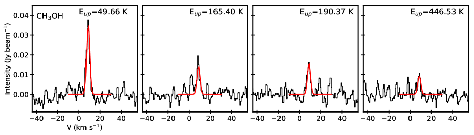
Figure 3: Gaussian fits in red to the observed CH₃OH lines in black (see Table 1) used to calculate the integrated flux density for Eq. B1

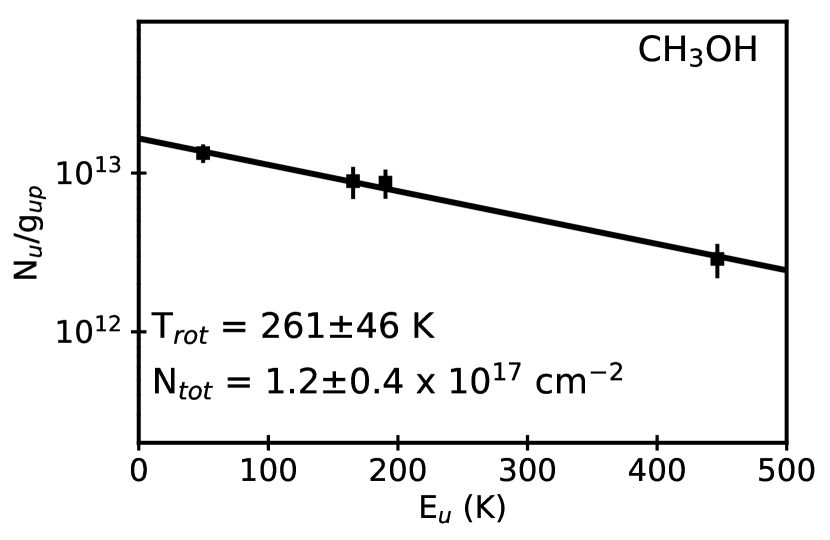
Figure 4: Rotational diagram for CH₃OH. The three squares correspond to the three detected transitions in our dataset (see Fig. 3). The plotted 1$\sigma$ errors include an additional 10% to the integrated flux density errors provided by the Gaussian fit to account for calibration errors, since we are using lines observed with two different frequency settings. The best fit to the data is represented by a solid line, and the derived rotational temperature and column density are indicated in the plot.

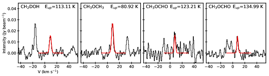
Figure 5: Gaussian fits in red to the observed CH₂DOH, and CH₃OCH₃, and CH₃OCHO lines (see Table 1) used to calculate the integrated flux density for Eq. B1.

For those species with more than one detected transition, the rotational diagram can be used to derive excitation temperatures and column densities (Goldsmith & Langer, 1999, , see Sect. B). Figure 4 shows the rotational diagram for CH₃OH using the spectrum extracted at the continuum peak. We attempted to perform similar calculations for other molecules, but a combination of low S/N and/or a lack of lines spanning a wide range of E_up resulted in unconstrained excitation temperatures and column densities.

To extract the CH₃OH line fluxes and flux uncertainties, we fitted a Gaussian to each observed CH₃OH line (see Fig. 3) using the Python function curve_fit with a fixed $V_{LSR}$ = 8.64 km s^-1, and FWHM = 3.33 km s^-1, corresponding to the position and width of the brightest methanol line detected. The integrated flux densities calculated from the Gaussian fits are roughly equal to the moment 0 peak intensities listed in Table 1. In Ser-emb 1, the methanol emission originates in a compact region around the protostar (see Sect. 3.3). For the images cleaned with a robustness parameter of 0.5 (where the spectrum has been extracted from), the size of the beam is $\Omega_{beam}$ = 0.55$\arcsec$ $\times$ 0.45$\arcsec$ (Table 4), while the size of the methanol emitting region is $\Omega_{source}$ $\leq$ (0.29 $\pm$ 0.15)$\arcsec$ $\times$ (0.12 $\pm$ 0.10)$\arcsec$. The source size was estimated with a 2D Gaussian fit of the 10_-3 $-$ 11_-2 moment 0 map after deconvolving the beam size. However, this estimated source size is the largest source size consistent with our observations, and the actual size of the methanol emitting region could be smaller. For the rotational diagram, we corrected the observed flux densities from beam dilution using the minimum filling factor of $\sim$7.5 in Eq. B1 that corresponds to the maximum source size. Therefore, the calculated column density should be considered a lower limit.

The rotational diagram fit was performed with the function curve_fit in Python. The derived column density for CH₃OH is $N_{T}$ = (1.2 $\pm$ 0.4) $\times$ 10¹⁷ cm^-2 (corresponding to the largest source size consistent with our observations), and the rotational temperature is $T_{rot}$ = 261 $\pm$ 46 K (i.e., $T_{rot}>$100 K, above the water ice desorption temperature). The optical thickness of the brightest detected line is $\tau$ = 0.1. Therefore, we expect the optically thin line assumption (Sect. B) to be valid for all observed transitions. We have also fitted the methanol rotational diagram excluding the brightest line (E_up = 49.66 K), and get the same column density and a rotational temperature. This suggests that the optical thickness of the 5_1- $-$ 4_1- line is not impacting the calculated column density. However, we note that these values should be considered lower limits, as stated above, since the actual size of the methanol emitting region could be smaller, increasing the column density up to a factor of 3 (Bergner et al., 2019). We therefore cannot completely exclude that the 5_1- $-$ 4_1- line is optically thick. Observations of more lines of CH₃OH and its isotopologs are needed to better constrain the methanol column density and address the optical depth issues.

We adopted the rotational temperature derived for CH₃OH to estimate the column densities of CH₂DOH and the two detected COMs, applying Eq. B2 to their brightest detected transition (see Fig. Fig. 5), and the same minimum filling factor as for CH₃OH, since we expect these species to emit from the same region (see Sect. 3.3). The results for CH₂DOH (using the 9_2,7,0 $-$ 9_2,7,0 transition), CH₃OCH₃ (treating the unresolved multiplet 13_0,13 $-$ 12_1,12 as a single line), and CH₃OCHO (averaging the total column density calculated from the two unblended transitions, since the strongest transition is blended) are presented in Table 2. We have corrected the CH₃OCHO column density by a factor of 2.1 (corresponding to a rotational temperature of 261 K) to take into account the higher torsional states that are not included in the partition function extracted from the JPL catalog (Favre et al., 2014). The estimated column densities are (4.8 $\pm$ 1.8) $\times$ 10¹⁶, (9.2 $\pm$ 3.8) $\times$ 10¹⁶, and (9.1 $\pm$ 3.6) $\times$ 10¹⁶, for CH₂DOH, CH₃OCH₃, and CH₃OCHO, respectively. Again, these values should be considered lower limits since we have used the minimum filling factor. These column densities imply a D/H ratio for methanol of 0.40, and CH₃OCH₃/CH₃OH and CH₃OCHO/CH₃OH ratios of 0.77 and 0.76, respectively. These ratios are high, and could be affected by the uncertainties in the estimation of the methanol column density explained above. If we instead used, for example, the D/H ratio recently reported for methanol in HH 212 (0.27, Lee et al., 2017), the CH₃OH column density would be 1.8 $\times$ 10¹⁷; while applying the D/H ratio found in B1b-S for methyl formate (0.02, Marcelino et al., 2018) to the CH₂DOH column density leads to a CH₃OH column density one order of magnitude higher (2.4 $\times$ 10¹⁸). In addition, we note that methanol emission often presents an extended component around protostars (see, e.g., Öberg et al., 2013), that could be filtered out in these kind of observations that lack short baselines, also leading to an underestimation of its column density. Therefore the reported ratios should be treated as upper limits.

Table 2: COMs column densities in the hot corino of Ser-emb 1.

Molecule	$N_{T}$	$N_{T}$/$N_{T}$(CH3OH)
	(molecules cm-2)
CH3OH	$\geq$(1.2 $\pm$ 0.4) $\times$ 1017	1.00
CH2DOH	$\geq$(4.8 $\pm$ 1.8) $\times$ 1016	0.40
CH3OCH3	$\geq$(9.2 $\pm$ 3.8) $\times$ 1016	0.77
CH3OCHO	$\geq$(9.1 $\pm$ 3.6) $\times$ 1016	0.76

Note. — These column densities are calculated assuming a maximum source size of $\Omega_{source}$ = (0.29 $\pm$ 0.15)$\arcsec$ $\times$ (0.12 $\pm$ 0.10)$\arcsec$, as extracted from a 2D Gaussian fit after deconvolving the beam size, and should therefore be considered lower limits (see text).

3.3 Spatial distributions

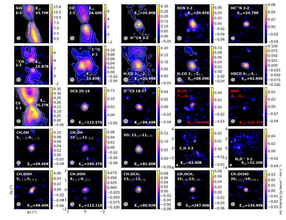
Figure 6: Integrated intensity (moment 0) maps, along with the 3, 6, 9, 12, 15, 18, 24, and 30$\sigma$ contours of some transitions identified toward the continuum peak of Ser-emb 1 (maps are clipped at 1$\sigma$). The rms for the contours is indicated in Table 1 for each line. The size of the synthesized beam ($\sim$ 0.50$\arcsec$ $\times$ 0.42$\arcsec$) is shown in the lower left of every panel (see also Sect. A).

To explore the spatial distributions of the detected molecules, the individual data cubes cleaned with a robustness parameter of 0.0 for a better angular resolution (Sect. 2.3) were integrated over the full line width of the emission lines. Fig. 6 shows the resulting integrated emission images (moment 0 maps) of all the molecules listed in Table 1. For molecules where multiple lines were detected with substantially different upper level energies, two lines are shown. The integrated intensity peaks and the moment 0 maps rms are listed in Table 1.

Among the small species (4 atoms or less) most, but not all, present emission extended over the the slow outflow region traced by the low-velocity CO 2 $-$ 1 emission (see Sect. 3.1), up to $\sim$4$\arcsec$ or $\sim$1600 au of the central protostar in the case of CS or H₂CO. The exceptions are, on one hand, N₂D⁺, whose emission is extended to the outer cold envelope where CO molecules are frozen onto the dust grains (see, e.g., Bergin et al., 2001), with no emission detected within $\sim$1$\arcsec$ or $\sim$400 au from the central protostar; and on the other hand, OCS and SO₂ that present only compact, barely resolved emission. By contrast, the emission of all organic molecules with 5 or more atoms is unresolved in a compact region around the protostar. CH₃OH and CH₂DOH are detected within $\sim$0.4$\arcsec$ or $\sim$160 au from the central protostar. The size of the emitting region for the 5_1,-,0 $-$ 4_1,-,0 methanol line, obtained with a 2D Gaussian fit after deconvolving the beam size, is (0.26 $\pm$ 0.08)$\arcsec$ x (0.12 $\pm$ 0.11)$\arcsec$ (this is actually the maximum source size consistent with the data, see Sect. 3.2.1). Methanol would be thus emitting within a radius of $\sim$50 au from the central protostar. The emission from CH₃OCH₃ and CH₃OCHO is contained within the beam size and it could not be deconvolved from the beam. The detection of these organic molecules in a compact region around the protostar is not only a matter of sensitivity, since the peak integrated intensity of some lines presenting only compact emission (e.g., CH₃OH 5_1,-,0 $-$ 4_1,-,0) is higher than that of some lines showing extended emission (e.g., H₂CO 3_2,2 $-$ 2_2,1, see Table 1). Therefore, CH₃OH and the two COMs CH₃OCH₃ and CH₃OCHO are present in a compact (the beam radius is $\sim$100 au, see Sect. 2.3), high-temperature region around the central protostar. This is consistent with the high excitation temperature of CH₃OH derived in the previous section.

3.4 Rotation signature

In Fig. 1, we show that the high-velocity C¹⁸O 2 $-$ 1 emission is compact, and spatially distributed from red- to blue-shifted velocities orthogonally to the direction of the outflow, which could be an indication of rotation of this molecule around the central object. We similarly plotted all detected lines and found a comparable velocity gradient in the H₂CO 3_0,3 $-$ 2_0,2 high-velocity map (Fig. 7). We note that the emission originating from CH₃OH and the CH₃OCH₃ and CH₃OCHO COMs appears unresolved, and a similar velocity pattern on smaller scales cannot be excluded.

A priori, a velocity gradient across a protostar can have several different origins: outflows (see Fig. 1), infall, and rotation. In the latter case, it is not given that rotation automatically implies the presence of a Keplerian (rotationally supported) disk around the central protostar, since it also trace the rotating motion of the infalling envelope. In Ser-emb 1, several aspects of the observed emission may point to the former as the origin of the velocity gradient. First, there is no sign of protostellar multiplicity and thus reason to expect a second outflow associated with this source Second, the velocity gradient is orthogonal to the observed outflow, which is assumed to be the axis of rotation of a potential protostellar disk. Third, the high-velocity emission showing the velocity gradient is very compact, i.e. only visible on scales associated with protostellar disks ($<$200 au radius). Still we cannot exclude from the maps alone that we are observing an infalling-rotating envelope rather than a rotationally supported disk (see, e.g., Tobin et al., 2012a; Oya et al., 2016, 2017; Jacobsen et al., 2019).

In order to further study these rotation signatures, the top panels of Fig. 8 show the position-velocity (PV) diagrams along the direction perpendicular to the outflow, for the two transitions in Fig. 7. The C¹⁸O 2 $-$ 1, and H₂CO 3_0,3 $-$ 2_0,2 lines show a spin-up feature toward the protostar. The spin-up feature consists in a velocity gradient from one side of the outflow axis to the other, with the red-shifted emission ($V_{LSR}$ $>$ 8.6 km s^-1, above the horizontal dashed line) mainly located to the east of the central protostar position (offset $>$ 0^′′, to the left of the vertical dashed line), and the blue-shifted emission ($V_{LSR}$ $<$ 8.6 km s^-1, below the horizontal dashed line) preferentially detected to the west (offset $<$ 0^′′, to the right of the vertical dashed line); and with higher velocities closer to the protostar. A similar feature in the PV diagram was also observed in Lee et al. (2017) for the red- and blue-shifted emission of CH₃OH and CH₂DOH, that could be reproduced with a Keplerian rotation model, thus indicating that these species trace the disk atmosphere in HH 212. In our case, a Keplerian rotation curve ($v\propto R^{-0.5}$, shown in red in Fig. 8) is able to reproduce the observed spin-up feature, but the model considering an infalling-rotating envelope ($v\propto R^{-1}$, shown in orange in Fig. 8) cannot be ruled out. On the other hand, the spin-up feature is not clearly observed in the PV diagrams along the direction of the outflow (bottom panels of Fig. 8), where red- and blue-shifted emission is more symmetrically detected to both the north (offset $>$ 0^′′) and the south (offset $<$ 0^′′) of the central protostar position. This cannot be reproduced by the same infalling-rotating envelope model ($v\propto R^{-1}$, shown in grey in Fig. 8) that would locate the red-shifted emission preferentially to the south of the source, and the blue-shifted emission to the north. However, these PV diagrams show non-negligible infall velocities along the minor axis of the potential protostellar disk (especially in the case of H₂CO), unlike methanol and deuterated methanol in Lee et al. (2017).

In summary, we have detected a rotation signature orthogonal to the outflow in two molecular lines, which are consistent Keplerian rotation, but observations with higher spatial resolution (and a higher signal-to-noise ratio) are needed to unambiguously distinguish from the rotating motion of the infalling envelope.

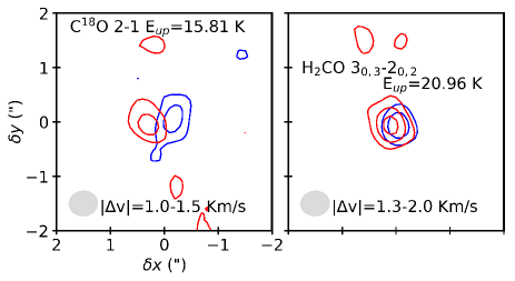
Figure 7: 3, 6, and 9$\sigma$ contours of the high-velocity blue- and red-shifted moment 0 maps corresponding to different molecular transitions showing spatially resolved blue- and red-shifted emission. The range of velocities with respect to $V_{LSR}$ is indicated in every panel. The size of the synthesized beam ($\sim$ 0.50$\arcsec$ $\times$ 0.42$\arcsec$) is shown in the lower left of every panel (see also Sect. A).

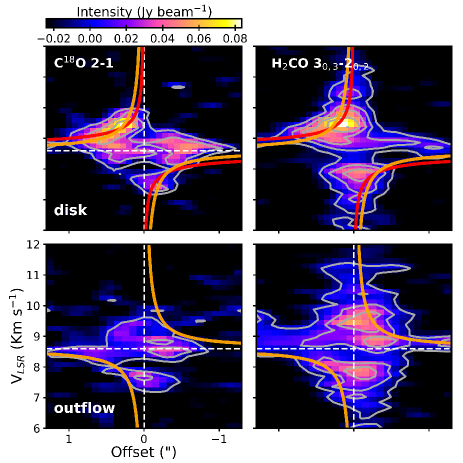
Figure 8: PV diagrams of a 0.24$\arcsec$ width slice along the direction perpendicular to the outflow (PA = -77.7^∘, top panels) and the direction of the outflow, assumed to be the axis of rotation (PA = 12.2^∘, bottom panels) at both sides of the continuum peak position (offset = 0^′′) corresponding to the molecular lines in Fig. 7. The position of the central protostar and the radial velocity of the source are indicated with dashed, white lines. The 3, 6, 9, 12, 15$\sigma$ contours are overlaid in grey (see Table 4 for the rms corresponding to each transition). Pure Keplerian ($v\propto R^{-0.5}$, red) and infall ($v\propto R^{-1}$, orange) curves are shown, when appropriate.

4 Discussion

4.1 Hot corino chemistry in Ser-emb 1

According to the definition in Herbst & van Dishoeck (2009), a warm inner envelope passively heated by the central protostar to typical temperatures around 100 K or warmer, with typical sizes of 100 au or less, associated with complex organic molecule emission is considered a hot corino. The presence of CH₃OH, CH₃OCH₃, and CH₃OCHO emitting in a compact region (beam radius $\sim$100 au, Sect. 2.3) around the central protostar in Ser-emb 1 (Sect. 3.3), with a measured rotational temperature for CH₃OH of $T_{rot}$ = 249 $\pm$ 42 K (Sect. 3.2.1) means that Ser-emb 1 fulfills the above criteria, with the addition that the hot corino could be associated to an incipient protostellar disk (see Sect. 3.4), as it is the case in, e.g., HH 212 (Lee et al., 2017; Codella et al., 2018; Lee et al., 2019).

As stated in Sect. 1, not all warm compact cores present a hot core/corino chemistry. Some sources show a different chemistry characterized by unsaturated carbon chains, and are usually known as warm carbon chain chemistry (WCCC) sources (see, e.g., Lefloch et al., 2018) While our observations do not constitute an unbiased survey, the non-detection of C₂H toward the central protostar position in Ser-emb 1 (Sect. 3.2) implies a hydrocarbon-poor, organic chemistry similar to other detected hot corinos.

Table 3: COMs column densities in Class 0 hot corinos. Sources with only single-dish observations are marked with a ^∗.

Source	$N$ ($\times$ 1016 cm-2)			Reference	L⊙	Reference
	CH3OH	CH3OCH3	CH3OCHO
IRAS 2A	500${}^{+290}_{-180}$	5.0${}^{+2.9}_{-1.0}$	7.9${}^{+4.6}_{-1.6}$	Taquet et al. (2015)	36	Karska et al. (2013)
IRAS 16293B	1000	24	26	Jørgensen et al. (2018)a	22	Crimier et al. (2010)
L483	1700	8.0	13	Jacobsen et al. (2019)	10-14	Jacobsen et al. (2019)
IRAS 4A2	$\cdots$	4.5${}^{+0.3}_{-0.2}$	3.5${}^{+0.2}_{-0.4}$	López-Sepulcre et al. (2017)	9.1	Karska et al. (2013)
HH 212	61.0$\pm$33.0	$\cdots$	3.2$\pm$1.2	Lee et al. (2019)	9	Zinnecker et al. (1992)
IRAS 4B∗	34.2b	$<$6.5c	8.9$\pm$6.5	Bottinelli et al. (2007)	6	Jørgensen et al. (2002)
Ser-emb 1d	12$\pm$4	9.2$\pm$3.8	9.1$\pm$3.6	This work	4.1	Enoch et al. (2011)
B335	$\cdots$	0.19$\pm$0.02	2.6$\pm$0.3	Imai et al. (2016)	0.72	Evans et al. (2015)
B1b-S	35	1.0	1.5	Marcelino et al. (2018)	0.49	Pezzuto et al. (2012)

Note. — ^aAt the position offset by 0.5$\arcsec$ from the continuum peak. Uncertainties are estimated to be about 20%. ^bFrom the CH₃OCHO/CH₃OH ratios in Herbst & van Dishoeck (2009). ^cFrom the CH₃OCH₃/CH₃OH ratio in Herbst & van Dishoeck (2009). ^dAssuming a source size of $\Omega_{source}$ = (0.29 $\pm$ 0.15)$\arcsec$ $\times$ (0.12 $\pm$ 0.10)$\arcsec$ (see Sect. 3.2.1).

Table 3 compares the estimated column densities of CH₃OH and the two COMs reported in this paper (CH₃OCH₃ and CH₃OCHO) in Ser-emb 1 with those reported in the literature for the other eight Class 0 hot corinos. The bolometric luminosities of the sources are also indicated. Roughly, the most luminous sources (IRAS 2A, IRAS 16293B, and L483) present methanol column densities on the order of $\sim$10^18-19, while the column densities estimated for the rest of hot corinos are on the order of $\sim$10¹⁷, cosnsitent with the value presented here for Ser-emb 1. On the other hand, the column densities of dimethyl ether and methyl formate present a larger scatter across the sample of Class 0 hot corinos, with no obvious trend. The COM abundances with respect to CH₃OH across the sample of detected hot corinos (and also the different evolutionary stages during star formation) are further discussed in Bergner et al. (2019).

4.2 A protostellar disk in Ser-emb 1?

Enoch et al. (2011) already suggested the presence of a partially resolved disk structure around the central protostar in Ser-emb 1 due to the substantial $\sim$230 GHz continuum flux detected at intermediate uv distances (30$-$100 k$\lambda$). This corresponds to a disk radius above 170 au, of the same order as other confirmed protostellar disks in Class 0 sources (50$-$150 au, Choi et al., 2010; Tobin et al., 2012b; Murillo et al., 2013; Yen et al., 2013; Codella et al., 2014; Lindberg et al., 2014; Oya et al., 2016; Yen et al., 2017; Lee et al., 2017). The value reported in Enoch et al. (2011) agrees well with our estimated radius of $\sim$200 au for the C¹⁸O high-velocity emission in Fig. 7. The disk mass estimated from the continuum flux at 50 k$\lambda$ is (0.28 $\pm$ 0.14) $M_{\odot}$ (Enoch et al., 2011), which is higher than the mass reported for the protostellar disk around, e.g., L1527 IRS (0.007 $M_{\odot}$, Tobin et al., 2012b), but of the same order as the disk in Lupus 3MMS (0.1 $M_{\odot}$, Yen et al., 2017). If confirmed, the size and mass of the rotating structure in Ser-emb 1 are comparable to other previously detected protostellar disks around Class 0 protostars.

The observed velocity gradient perpendicular to the outflow in, especially, C¹⁸O, and the spin-up features apparent in its PV diagram are consistent with Keplerian rotation, similar to what has been observed for other Class 0 protostellar disks (e.g., HH 212 in Lee et al., 2017). While a contribution from infalling envelope material cannot be excluded in Ser-emb 1, our PV diagrams are more comparable to the three-dimensional model of Keplerian rotation shown in Oya et al. (2016, 2017) for the COM emission in IRAS 16293A and L483, respectively, than to their corresponding models for infalling-rotating envelopes. In summary, this model predicts a spin-up feature only in the PV diagram along the direction perpendicular to the outflow, and symmetric, diamond-shaped emission for the PV diagram in the direction of the outflow for a Keplerian disk (similarly to what is observed for C¹⁸O and H₂CO in Fig. 8); while a model of an infalling-rotating envelope should present a spin-up feature in both the PV diagrams prependicular to the outflow and along the direction of the outflow. However, better spatial resolution observations have recently ruled out the presence of a protostellar disk in L483, even when their infalling-rotating envelope model alone could not reproduce the features of the observed PV diagrams. Higher spatial resolution and higher signal-to-noise ratio data are therefore needed to confirm the nature of the rotating structure in Ser-emb 1, and elucidate whether it is a pseudodisk or a fully rotationally supported disk).

The spatial coincidence of the compact hot corino emission and the candidate protostellar disk in Ser-emb 1 implies that the hot corino may be a warm disk. Including Ser-emb 1, four out of the ten detected hot corino sources are candidates to harbor rotationally supported protostellar disks (the others being IRAS 4A2, HH212, and IRAS 16293A, as explained in Sect. 1). Therefore, the hot corino chemistry in low-mass protostars could be located in the incipient protostellar disks formed as the result of the angular momentum conservation of the infalling envelope, as seen for the above mentioned sources in Oya et al. (2016); Lee et al. (2017); Codella et al. (2018); Lee et al. (2019), which would have important implications regarding the incorporation of precursors for prebiotic molecules to the planet-forming disks.

5 Conclusions

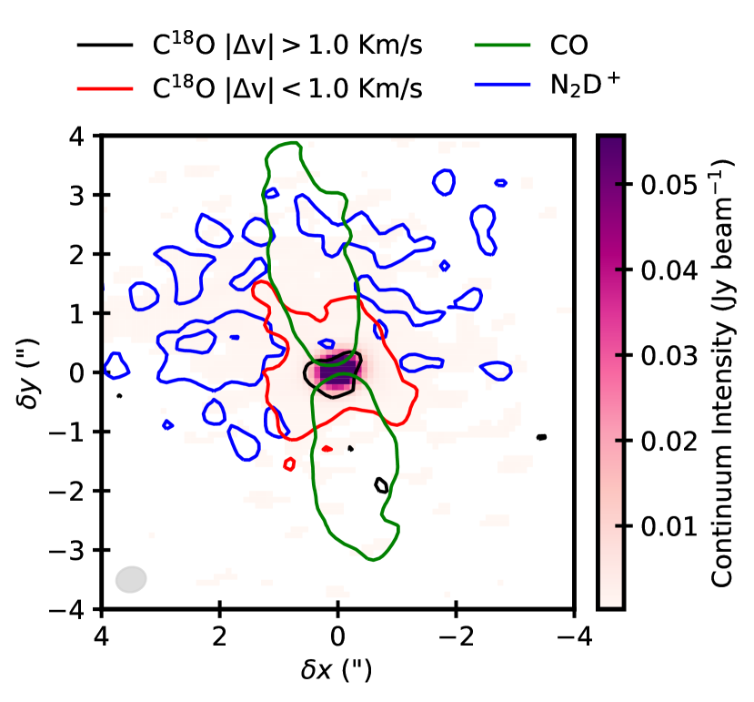
Figure 9: Overview of the Ser-emb 1 source. The continuum map at 232 GHz traces the dust emission around the central protostar. The 6$\sigma$ contour of the CO 2 $-$ 1 moment 0 map is presented in green, tracing the bipolar jet and outflowt. The 5$\sigma$ contour of the moment 0 map encompassing the mid- and low-velocity channels (up to $\sim$1.0 km/s away from the $V_{LSR}$) of the C¹⁸O 2 $-$ 1 line is shown in red, and trace the slow outflow; while the 4$\sigma$ contour high-velocity channels (from $\sim$1.0 to $\sim$1.5 km/s away from the $V_{LSR}$) in black trace the compact molecular emission. Finally, the 2$\sigma$ contours of the N₂D+ 3 $-$ 2 moment 0 map are shown in blue, and trace the cold outer envelope. The size of the synthesized beam ($\sim$ 0.50$\arcsec$ $\times$ 0.42$\arcsec$) for the continuum map is shown in the lower left (see also Sect. A)

1. The different species detected in our observational dataset trace chemically distinct structural components of the Ser-emb 1 YSO. These components can be observed in Fig. 9, and consist of the central protostar, traced by the dust continuum map at 232 GHz; a rotating compact emission in the close vicinity of the central object, traced by the C¹⁸O 2 $-$ 1 velocity wings (black); a slow outflow traced by C¹⁸O (red); a bipolar jet and outflow, traced by the CO 2 $-$ 1 emission (green); and the cold outer envelope, traced by the N₂D⁺ 3 $-$ 2 line (blue).

2. In particular, we have detected ten chemically distinct species (and seven isotoplogs) with emission toward the continuum peak of Ser-emb 1 (Table 1), including the COM precursors H₂CO and CH₃OH, and two COMs: CH₃OCH₃, and CH₃OCHO.

3. The rotational diagram analysis of the four CH₃OH lines results in a rotational temperature of $T_{rot}$ = 261 $\pm$ 46 K. The compact (radius $<$100 au) emission coming from CH₃OH, CH₃OCH₃, and CH₃OCHO, with a temperature above the ice sublimation temperature, implies that Ser-emb 1 harbors a hot corino. Additional unbiased observations are required to determine its full chemical richness.

4. The high-velocity moment 0 maps of the C¹⁸O 2 $-$ 1, and H₂CO 3_0,3 $-$ 2_0,2 transitions present spatially resolved blue- and red-shifted emission orthogonally to the outflow direction, indicative of rotation around the central protostar. The PV diagrams of the C¹⁸O and H₂CO transitions along this direction and the direction of the outflow are consistent with a disk-like structure with radius $<$200 au, but contribution from the infalling-rotating envelope cannot be completely excluded.

5. The spatial coincidence of the hot corino emission and the potential protostellar disk suggest that the hot corino could be actually a warm disk. Further observations with better spatial resolution and higher sensitivity of CH₃OH and other COMs are needed to evaluate this scenario.

Appendix A Observed spectral windows

Table 4: Spectral windows observed with the two correlator setups described in Sect. 2. For each spectral window, the first row corresponds to the channel rms and beam size reached after cleaning the data cube with a robustness parameter of 0.5; while the second row corresponds to the individually imaged transitions detected in the spectral windows, cleaned with robust = 0.0.

Frequency range	$\Delta$V	Channel rms	Beam size
(GHz)	(km s-1)	(mJy beam-1)	′′
217.209 $-$ 217.268	0.168	5.9	0.62 $\times$ 0.52
		7.5	0.54 $\times$ 0.48
218.193 $-$ 218.251	0.168	5.1	0.61 $\times$ 0.52
		6.7	0.53 $\times$ 0.48
218.446 $-$ 218.505	0.168	5.0	0.61 $\times$ 0.52
		6.4	0.53 $\times$ 0.48
218.703 $-$ 218.762	0.167	5.1	0.61 $\times$ 0.52
		$\cdots$ (a)	$\cdots$ (a)
219.502 $-$ 219.619	0.167	6.3	0.62 $\times$ 0.50
		7.0	0.53 $\times$ 0.46
220.340 $-$ 220.457	0.167	9.1	0.62 $\times$ 0.50
		9.2	0.53 $\times$ 0.46
230.479 $-$ 230.597	0.159	9.1	0.65 $\times$ 0.48
		12.2	0.54 $\times$ 0.45
231.262 $-$ 231.380	0.158	6.8	0.58 $\times$ 0.47
		$\cdots$ (a)	$\cdots$ (a)
231.481 $-$ 233.356	0.630	2.0	0.58 $\times$ 0.46
		2.7	0.50 $\times$ 0.41
242.978 $-$ 244.853	0.600	2.3	0.55 $\times$ 0.45
		2.8	0.47 $\times$ 0.40
244.164 $-$ 244.281	0.150	6.1	0.56 $\times$ 0.47
		8.2	0.50 $\times$ 0.40
244.877 $-$ 244.994	0.149	5.8	0.56 $\times$ 0.47
		7.3	0.50 $\times$ 0.40
258.098 $-$ 258.216	0.142	6.3	0.52 $\times$ 0.44
		8.3	0.45 $\times$ 0.39
258.953 $-$ 259.070	0.141	5.8	0.51 $\times$ 0.44
		7.5	0.45 $\times$ 0.39
260.459 $-$ 260.577	0.140	6.7	0.51 $\times$ 0.43
		8.5	0.45 $\times$ 0.38
262.150 $-$ 262.267	0.140	7.3	0.51 $\times$ 0.43
		8.4	0.44 $\times$ 0.38

• ^(a)No individual transitions were imaged with a robust = 0.0 in these spectral windows.

Appendix B Rotational diagram

Assuming local thermodynamical equilibrium (LTE) and optically thin lines, the integrated flux density $\int{S_{\nu}dv}$ of a given transition is related to the population of the corresponding upper level $N_{u}$ by Eq. B1:

$$N_{u}=\frac{4\pi\int{S_{\nu}dv}}{A_{ul}\Omega hc},$$ (B1)

where $A_{ul}$ is the Einstein coefficient of the transition (indicated in Table 1 for every detected transition in our dataset), $\Omega$ is the solid angle subtended by the emitting region, $h$ is the Planck constant, and $c$ the speed of light.

For the spectra in Figures 3 and 5, $\Omega$ is assumed to be the beam solid angle. If the emitting region is smaller than the beam size, the observed integrated flux density is diluted in the beam. To correct for this beam dilution we have to apply the filling factor $\frac{\Omega_{beam}}{\Omega_{source}}$ to Eq. B1

The upper level population $N_{u}$ is related to the total column density $N_{T}$ of the species according to the Boltzmann equation:

$$\frac{N_{u}}{g_{up}}=\frac{N_{T}}{Q(T_{rot})}e^{-E_{up}/T_{rot}},$$ (B2)

where $g_{up}$ and $E_{up}$ are the upper level degeneracy and upper level energy in K of the transition, respectively (also indicated in Table 1 for the detected transitions), $T_{rot}$ the rotational temperature, and $Q(T_{rot})$ the partition function of the species (extracted from the JPL catalog). This way, every observed line represents one point in the rotational diagram of a species. Taking the natural logarithm of Eq. B2 leads to:

$$ln\frac{N_{u}}{g_{up}}=ln\frac{N_{T}}{Q(T_{rot})}-\frac{E_{up}}{T_{rot}}.$$ (B3)

Therefore, if $\frac{N_{u}}{g_{up}}$ of the different detected transitions of a given species are semi-log plotted against their upper level energies $E_{up}$, the rotational diagram can be fitted with a linear least squares regression, where $T_{rot}$ is the inverse of the slope and $N_{T}$ can be calculated from the intercept of the fit.

References

- André et al. (1993) Andreé, P., Ward-Thompson, D., & Barsony, M. 1993, ApJ, 406, 122
- Arce et al. (2008) Arce, H. G., Santiago-García, J., Jørgensen, J. K., Tafalla, M., & Bachiller, R. 2008, ApJ, 681, L21
- Bergin et al. (2001) Bergin, E.A., Ciardi, D.R., Lada, C.J., Alves, J., & Lada, E.A. 2001, ApJ, 557, 209
- Bergner et al. (2017) Bergner, J.B., Öberg, K.I., Garrod, R.T., & Graninger, D.M. 2017, ApJ, 841, 2, id.120
- Bergner et al. (2019) Bergner, J.B., Martín-Doménech, R., Öberg, K.I., et al. 2019, submitted
- Bianchi et al. (2019) Bianchi, E., Codella, C., Ceccarelli, C., et al. 2019, MNRAS, 483, 2, 1850
- Bottinelli et al. (2004) Bottinelli, S., Ceccarelli, C., Lefloch, B., et al. 2004, ApJ, 615, 354
- Bottinelli et al. (2007) Bottinelli, S., Ceccarelli, C., Williams, J. P., & Lefloch, B. 2007. A&A, 463, 601
- Cazaux et al. (2003) Cazaux, S., Tielens, A. G. G. M., Ceccarelli, C., et al. 2003, ApJ, 593, L51
- Choi et al. (2010) Choi, M., Tatematsu, K., & Kang, M. 2010, ApJ, 723, L34
- Codella et al. (2018) Codella, C., Bianchi, E., Tabone, B., et al. 2018, A&A, 617, A10
- Codella et al. (2014) Codella, C., Cabrit, S., Gueth, F., et al. 2014, A&A, 568, L5
- Codella et al. (2016) Codella, C., Ceccarelli, C., Cabrit, S., et al. 2016, A&A, 586, L3
- Codella et al. (2017) Codella, C., Ceccarelli, C., Caselli, P., et al. 2017, A&A, 605, L3
- Crimier et al. (2010) Crimier, N., Ceccarelli, C., Maret, S., et al. 2010, A&A, 519, A65
- Endres et al. (2009) Endres, C.P., Drouin, B.J., Pearson, J.C., et al. 2009, A&A, 504, 635
- Enoch et al. (2011) Enoch, M. L., Corder, S., Duchêne, G., et al. 2011, ApJS, 195, 21
- Enoch et al. (2009) Enoch, M. L., Evans, N. J., II, Sargent, A. I., & Glenn, J. 2009, ApJ, 692, 973
- Evans et al. (2015) Evans, N. J., II, Di Francesco, J., Lee, J., et al. 2015, ApJ, 814, 22
- Favre et al. (2014) Favre, C., Carvajal, M., Field, D., et al. 2014, ApJSS, 215, 2, id25
- Garrod et al. (2006) Garrod, R. T., Widicius Weaver, S.L., & Herbst, E. 2006, ApJ, 682, 1, 283
- Garrod et al. (2008) Garrod, R. T., & Herbst, E. 2008, ApJ, 457, 3, 927
- Goldsmith & Langer (1999) Goldsmith, P.F., & Langer, W.D. 1999, ApJ, 517, 209
- Herbst & van Dishoeck (2009) Herbst, E., & van Dishoeck, E.F. 2009, ARA&A, 47, 427
- Ilyushin et al. (2009) Ilyushin, V., Kryvda, A., & Alekseev, E. 2009, J. Mol. Spectrosc., 255, 32
- Imai et al. (2016) Imai, M., Sakai, N., Oya, Y., et al. 2016, ApJ, 830, L37
- Jacobsen et al. (2019) Jacobsen, S.K., Jørgensen, J.K., Di Francesco, J., et al. 2019, A&A, in press
-
Jiménez-Serra et al. (2016)
Jiménez-Serra, I., Vasyunin, A.I., Caselli, P., et al. 2016, ApJ, 830, 1, L6
- Jørgensen et al. (2005) Jørgensen, J.K., Bourke, T.L., Myers, P.C., et al. 2005, ApJ, 632, 973
- Jørgensen et al. (2018) Jørgensen, J.K., Müller, H.S.P., Calcutt, H., et al. 2018, A&A, 620, A170
- Jørgensen et al. (2002) Jørgensen, J. K., Schöier, F. L., & van Dishoeck, E. F. 2002, A&A, 389, 908
- Karska et al. (2013) Karska, A., Herczeg, G.J., van Dishoeck, E.F., et al. 2013, A&A, 552, A141
- Lee et al. (2019) Lee, C-F., Codella, C., Li, Z.-Y., & Liu, S.-Y. 2019, ApJ, accepted
- Lee et al. (2014) Lee, C-F., Hirano, N., Zhang, Q., et al. 2014, ApJ, 786, 114
- Lee et al. (2017) Lee, C-F., Li, Z.-Y., Ho, P.T.P., et al. 2017, ApJ, 843, 27
- Lefloch et al. (2018) Lefloch, B., Bachiller, R., Ceccarelli, C., et al. 2018, MNRAS, 477, 4792
- Lindberg et al. (2014) Lindberg, J. E., Jorgensen, J. K., Brinch, C., et al. 2014, A&A, 566, A74
- López-Sepulcre et al. (2017) López-Sepulcre, A., Sakai, N., Neri, R., et al. 2017, A&A, 606, A121
- Marcelino et al. (2007) Marcelino, N., Cernicharo, J., Agúndez, M. et al. 2007, ApJ, 665, L127
- Marcelino et al. (2018) Marcelino, N., Guerin, M., Cernicharo, J., et al. 2018, A&A, 620, A80
- McMullin et al. (2007) McMullin, J.P., Waters, B., Schiebel, D., Young, W., & Golap, K. 2007, ASPC, 376, 127
- Müller et al. (2005) Müller, H. S. P., Schlöder, F., Stutzki, J., & Winnewisser, G. 2005, JMoSt 742, 215
- Murillo et al. (2013) Murillo, N. M., Lai, S.-P., Bruderer, S., Harsono, D., & van Dishoeck, E. F. 2013, A&A, 560, A103
- Öberg et al. (2010) Öberg, K. I., Bottinelli, S., Jorgensen, J. K., & van Dishoeck, E. F. 2010, ApJ, 716, 1, 825
- Öberg et al. (2009) Öberg, K.I., Garrod, R.T., van Dishoeck, E.F., & Linnartz, H. 2009, A&A, 504, 3, 891
- Öberg et al. (2013) Öberg, K.I., Lauck, T., & Graninger, D. 2013, ApJ, 788, 68
- Ortiz-León et al. (2018) Ortiz-León, G.N., Loinard, L., Dzib, S.A., et al. 2018, ApJ, accepted
- Oya et al. (2015) Oya, Y., Sakai, N., Lefloch, B., et al. 2015, ApJ, 812, 59
- Oya et al. (2016) Oya, Y., Sakai, N., López-Sepulcre, A., et al. 2016, ApJ, 824, 88
- Oya et al. (2014) Oya, Y., Sakai, N., Sakai, T., et al. 2014, ApJ, 795, 152
- Oya et al. (2017) Oya, Y., Sakai, N., Watanabe, Y., et al. 2017, ApJ, 837, 174
- Pearson et al. (2012) Pearson, J.C., Yu, S., & Drouin, B.J. 2012, J. Mol. Spectros., 280, 119
- Pezzuto et al. (2012) Pezzuto, S., Elia, D., Schisano, E., et al. 2012, A&A 547, A54
- Pickett et al. (1998) Pickett, H. M., Poynter, R. L., Cohen, E. A., et al. 1998, JQSRT, 60, 883
- Rivilla et al. (2016) Rivilla, V.M., Fontani, F., Beltrán, M.T., et al. 2016, ApJ, 826, 2
- Rivilla et al. (2017) Rivilla, V. M. and Beltrán, M. T., Cesaroni, R., et al. 2017, A&A, 598, A59
- Robitaille et al. (2006) Robitaille, T. P., Whitney, B. A., Indebetouw, R., Wood, K., & Denzmore, P. 2006 ApJS, 167, 256
- Sakai et al. (2009) Sakai, N., Sakai, T., Hirota, T., Burton, M., & Yamamoto, S. 2009, ApJ, 697, 769
- Taquet et al. (2015) Taquet, V., López-Sepulcre, A., Ceccarelli, C., et al. 2015, ApJ, 804, 81
- Tobin et al. (2012a) Tobin J. J., Hartmann, L., Bergin, E., et al. 2012a, ApJ, 748, 16
- Tobin et al. (2012b) Tobin J. J., Hartmann, L., Chiang, H.-F., et al. 2012b, Natur, 492, 83
- Vastel et al. (2014) Vastel, C., Ceccarelli, C., Lefloch, B., & Bachiller, R. 2014, ApJ, 795, 1, L2.
- Xu et al. (2008) Xu. L.-H., Fisher, J., Lees, H.Y., et al. 2008, J. Mol. Spectrosc. 251, 305
- Yen et al. (2017) Yen, H.-W., Koch, P.M., Takakuwa, S., et al. 2017, ApJ, 834, 178
- Yen et al. (2013) Yen, H.-W., Takakuwa, S., Ohashi, N., & Ho, P.T.P. 2013, ApJ, 772, 22
- Zinnecker et al. (1992) Zinnecker, H., McCaughrean, M. J., & Rayner, J. T. 1998, Natur, 394, 862