Time-independent approximations for time-dependent optical potentials

Abstract:

We explore the possibility of modifying the Lewis-Riesenfeld method of invariants developed originally to find exact solutions for time-dependent quantum mechanical systems for the situation in which an exact invariant can be constructed, but the subsequently resulting time-independent eigenvalue system is not solvable exactly. We propose to carry out this step in an approximate fashion, such as employing standard time-independent perturbation theory or the WKB approximation, and subsequently feeding the resulting approximated expressions back into the time-dependent scheme. We illustrate the quality of this approach by contrasting an exactly solvable solution to one obtained with a perturbatively carried out second step for two types of explicitly time-dependent optical potentials.

1 Introduction

Since Ashkin’s discovery of the fact that radiation pressure from continuous lasers can be used to trap small particles, almost fifty years ago [1], various types of optical traps have been designed [2]. Different variants of optical traps have found widespead applications to fixate particles [3], atoms [4], molecules [5], and even living cells such as viruses and bacteria [6, 7]. Once the objects are fixed in the potential their properties can be investigated in a very controlled and otherwise inaccessible manner. The general underlying fundamental quantum mechanical description is provided by the time-dependent Schrödinger equation (TDSE) involving explicitly time-dependent Hamiltonians in which the optical potentials typically take on the generic form $V(x,t)=\kappa(t)V(x)$, with $V(x)$ describing the trapping shape and $\kappa(t)$ some time-dependent modulation, e.g. [8]. There exist, however, also optical potentials that can not be factorised in this manner, such as for instance periodic optical lattices [9].

In general, there are only very few exact solutions known to the TDSE and for many physical applications one relies predominatly on approximation methods. Most approximation methods for time-dependent systems are carried out on the level of the time-evolution operator, such as the adiabatic and the sudden approximation [10]. In more concrete settings less general approximation methods have been developed to account for the specifics of the system. For instance, a very active field of research involving time-dependent Hamiltonians is the area of strong laser fields [11]. The systems considered in this context involve Stark potentials of the form $V(x)+xE(t)$, with $E(t)$ describing a laser field and the term $xE(t)$ dominating or being comparable in strength to the potential $V(x)$. For these scenarios approximation schemes have been developed as a mixture of perturbative expansions based on the Du-Hamel formula carried out for time-evolution operator [12, 13, 14]. When iterated, these expressions give rise to various versions of the Born series. In the high intensity regime the two perturbative series, one in $V(x)$ and the other in $xE(t)$, are mixed and terminated after the first iteration. The expressions obtained in this manner are commonly referred to as the strong field approximation [15, 16, 17, 11].

There are, however, methods purposefully designed to solve the TDSE exactly. The Lewis-Riesenfeld method of invariants [18] is one of them. This scheme has been applied successfully to many models and scenarios, such as the harmonic oscillator with time-dependent mass and frequency in one [19] and two dimensions [20, 21], the damped harmonic oscillator [22], a time-dependent Coulomb potential [23], a time-dependent Hamiltonians given in terms of linear combinations of SU(1,1) and SU(2) generators [24, 25, 26], in the inverse construction of time-dependent Hamiltonian [27, 28], for systems on noncommutative spaces in time-dependent backgrounds [29], time-dependent non-Hermitian Hamiltonian systems [30, 31, 32, 33] and other specific systems.

Even though many exact solutions were found, in comparison they are still rare and for more involved potentials the method appears to be nonapplicable. This is partly due to the attempt to complete the Lewis and Riesenfeld method in its entirety. Here we propose to exploit a particular feature of the scheme and modify it when it can only be completed partially. In essence the method consists of three steps, of which often only the first step, that is the construction of the invariants, can be completed. Instead of abandoning the scheme one should recognize that with the completion of the first step one has achieved a major simplification and has transformed the system from a time-dependent first order differential equation to a time-independent eigenvalue equation. Usually one demands in the next step the solvability for this time-independent system, which again is a rare property. For many concrete optical potentials this seems to be entirely unachievable. We explore here the possibility of not terminating the procedure at this stage, but instead to use perturbative theory or the WKB approximation and subsequently feed the approximated expressions back into the Lewis-Riesenfeld approach. Naturally one may also use other approximation methods at this point.

We study here two concrete examples of optical potentials for which an exact method may be obtained and then compare it to the result for which the second step of the Lewis and Riesenfeld method has only been carried out perturbatively. Our manuscript is organised as follows: In section 2 we briefly recall the Lewis-Riesenfeld method of invariants and describe our proposal of altering the second step in the scheme. In section 3 and 4 we investigate in detail two concrete classes of optical potentials. The potentials are chosen in such a way that the full scheme can be completed, hence allowing a comparison with the approximated approach. Our conclusion and an outlook into future problems is provided in section 5.

2 An approximate Lewis-Riesenfeld method of invariants

We start by recalling the key steps of the method of invariants and then describe how they can be modified in an appropriate fashion. The scheme was introduced originally by Lewis and Riesenfeld [18], for the purpose of solving the TDSE

$$i\hbar\partial_{t}\left|\psi_{n}\right\rangle=H(t)\left|\psi_{n}\right\rangle,$$ (1)

for the time-dependent or dressed states $\left|\psi_{n}\right\rangle$ associated to the explicitly time-dependent Hamiltonian $H(t)$.

The Lewis-Riesenfeld method of invariants is made up of three main stages: The initial step in this approach consists of constructing a time-dependent invariant $I(t)$ from the evolution equation

$$\frac{dI(t)}{dt}=\partial_{t}I(t)+\frac{1}{i\hbar}[I(t),H(t)]=0.$$ (2)

Often this step can be completed and an exact form for the invariant $I(t)$ can be found. In the next step one needs to solve the corresponding eigenvalue system of the invariant $I(t)$

$$I(t)\left|\phi_{n}\right\rangle=\lambda_{n}\left|\phi_{n}\right\rangle,$$ (3)

for time-independent eigenvalues $\lambda_{n}$ and for the time-dependent states $\left|\phi_{n}\right\rangle$. Provided the Hamiltonian $H(t)$ is Hermitian also the invariant $I(t)$ is Hermitian and therefore the eigenvalues $\lambda_{n}$ are guaranteed to be real. The virtue of this equation, compared to the TDSE in (1), is that one has reduced the original evolutionary problem in form of a first order differential equation to an eigenvalue equation in which $t$ simply plays the role of a parameter. Hence one just needs to solve a time-independent eigenvalue problem. To complete this step the system in (3) needs to be solvable. It is this requirement one can weaken and employ time-independent approximation methods to complete step two.

The final third step relates the eigenstates in (3) with the complete solution of the TDSE. It was shown in [18] that the states

$$\left|\psi_{n}\right\rangle=e^{i\alpha_{n}(t)}\left|\phi_{n}\right\rangle$$ (4)

satisfy the TDSE (1) provided that the real function $\alpha(t)$ in (4) obeys

$$\frac{d\alpha(t)}{dt}=\frac{1}{\hbar}\left\langle\phi_{n}\right|i\hbar\partial_{t}-H(t)\left|\phi_{n}\right\rangle.$$ (5)

Since all the quantities on the right hand side of (5) have been obtained in the previous steps, one is left with a simple integration in time to determine the phase $\alpha(t)$. These key equations serve mainly for reference purposes and we refer the reader to [18] for more details.

For many systems we might succeed in carrying out the first step in the procedure and construct an explicit expression for the invariant $I(t)$. However, the process stalls often in the second step and for most Hamiltonians the eigenvalue equation for the invariants $I(t)$ in (3) can not be solved exactly. In this case we can, however, use approximation methods. For instance, when the potential can be separated into two terms, with one being dominating the other in absolute value, we can set up a standard time-independent perturbation theory. For this purpose let us briefly recall the main formulae in this approach.

We are splitting the invariant as

$$I(t)=I_{0}(t)+\epsilon I_{p}(t),$$ (6)

and consider the eigenvalue equation for the full invariant and the unperturbed one sparately

$$I(t)\left|\phi_{n}\right\rangle=\lambda_{n}\left|\phi_{n}\right\rangle,\qquad\text{and\qquad}I_{0}(t)\left|\phi_{n}^{(0)}\right\rangle=\lambda_{n}^{(0)}\left|\phi_{n}^{(0)}\right\rangle.$$ (7)

Assuming that within the perturbation term a small parameter $\epsilon\ll 1$ can be identified, we expand the eigenvalues and the eigenfunctions of the unperturbed invariant as

$$\lambda_{n}=\lambda_{n}^{(0)}+\epsilon\lambda_{n}^{(1)}+\epsilon^{2}\lambda_{n}^{(2)}+\mathcal{O}(\epsilon^{3}),\quad\text{and\quad}\left|\phi_{n}\right\rangle=\left|\phi_{n}^{(0)}\right\rangle+\epsilon\left|\phi_{n}^{(1)}\right\rangle+\epsilon^{2}\left|\phi_{n}^{(2)}\right\rangle+\mathcal{O}(\epsilon^{3}),$$ (8)

with $\lambda_{n}^{(k)}=1/k!\left.d\lambda_{n}/d\epsilon^{k}\right|_{\epsilon=0}$, $\left|\phi_{n}^{(k)}\right\rangle=1/k!\left.d\phi_{n}/d\epsilon^{k}\right|_{\epsilon=0}$. The first order corrections to the eigenvalues and eigenstates of the invariants are then computed in the standard fashion to

$$\lambda_{n}^{(1)}=\left\langle\phi_{n}^{(0)}\right|I_{p}\left|\phi_{n}^{(0)}\right\rangle,\quad\text{and\quad}\left|\phi_{n}^{(1)}\right\rangle=\sum\nolimits_{k\neq n}\frac{\left\langle\phi_{k}^{(0)}\right|I_{p}\left|\phi_{n}^{(0)}\right\rangle}{\lambda_{n}^{(0)}-\lambda_{k}^{(0)}}\left|\phi_{k}^{(0)}\right\rangle,$$ (9)

respectively. For orthonormal functions $\phi_{n}$, we obtain further constraints on the normalization of contributions in the series

$$1=\left\langle\phi_{n}\right.\left|\phi_{n}\right\rangle=\left\langle\phi_{n}^{(0)}\right.\left|\phi_{n}^{(0)}\right\rangle +\epsilon\left(\left\langle\phi_{n}^{(0)}\right.\left|\phi_{n}^{(1)}\right\rangle+\left\langle\phi_{n}^{(1)}\right.\left|\phi_{n}^{(0)}\right\rangle\right)$$ (11)

$$+\epsilon^{2}\left(\left\langle\phi_{n}^{(2)}\right.\left|\phi_{n}^{(1)}\right\rangle+\left\langle\phi_{n}^{(1)}\right.\left|\phi_{n}^{(1)}\right\rangle+\left\langle\phi_{n}^{(0)}\right.\left|\phi_{n}^{(2)}\right\rangle\right)+\ldots~{}~{}~{}~{}$$

Thus if the zero order wavefunction is normalized to $1=\left\langle\phi_{n}^{(0)}\right.\left|\phi_{n}^{(0)}\right\rangle$, we require the higher order wave functions to satisfy the additional constraints

$$\sum\limits_{k=0}^{\ell}\left\langle\phi_{n}^{(\ell-k)}\right.\left|\phi_{n}^{(k)}\right\rangle=0.$$ (12)

Next we can use these expressions to obtain an approximate solution to the TDSE. Denoting $\left|\phi_{n}\right\rangle^{(1)}:=\left|\phi_{n}^{(0)}\right\rangle+\epsilon\left|\phi_{n}^{(1)}\right\rangle$ we obtain

$$\left|\psi_{n}\right\rangle^{(1)}=e^{i\alpha_{n}^{(1)}(t)}\left|\phi_{n}\right\rangle^{(1)},\quad\text{and\quad}\alpha^{(1)}(t)=\frac{1}{\hbar}\int dt\,^{(1)}\!\left\langle\phi_{n}\right|i\hbar\partial_{t}-H(t)\left|\phi_{n}\right\rangle^{(1)}\text{.}$$ (13)

Alternatively, we may also solve the eigenvalue equation (3) by using the WKB approximation $\left|\phi_{n}^{\text{WKB}}\right\rangle$ and compute the phase using that expression

$$\left|\psi_{n}^{\text{WKB}}\right\rangle=e^{i\alpha_{n}^{\text{WKB}}(t)}\left|\phi_{n}^{\text{WKB}}\right\rangle,\quad\text{and\quad}\alpha^{\text{WKB}}(t)=\frac{1}{\hbar}\int dt\left\langle\phi_{n}^{\text{WKB}}\right|i\hbar\partial_{t}-H(t)\left|\phi_{n}^{\text{WKB}}\right\rangle.$$ (14)

Assuming that invariant $I(t)$ can be cast into the same form as a time-independent Hamiltonian, with a stndard kinetic energy term and a potential $V(\xi)$, the WKB approximation to first order in $\hbar$, see e.g. [34], for the eigenvalue equation (3) reads

$$\hat{\phi}^{\text{WKB}}(\xi)=\frac{A}{\sqrt{p(\xi)}}e^{\frac{i}{\hbar}\int^{\xi}p(z)dz}+\frac{B}{\sqrt{p(\xi)}}e^{-\frac{i}{\hbar}\int^{\xi}p(z)zx}$$ (15)

in the classically allowed region, $\lambda>V(\xi)$ and

$$\hat{\phi}^{\text{WKB}}(\xi)=\frac{C}{\sqrt{q(\xi)}}e^{\frac{1}{\hbar}\int^{\xi}q(z)dz}+\frac{D}{\sqrt{q(\xi)}}e^{-\frac{1}{\hbar}\int^{\xi}q(z)dz}$$ (16)

in the classically forbidden region $\lambda<V(\xi)$, where

$$p(\xi):=\sqrt{2[\lambda-V(\xi)]}\quad\text{and\quad}q(\xi):=\sqrt{2[V(\xi)-\lambda]}.$$ (17)

The constants $A$, $B$, $C$, $D$ need to be determined by the appropriate asymptotic WKB matching and the normalisation conditions.

Let us now apply this approximation scheme to some concrete systems.

3 Time-dependent potentials with a Stark term

We first demonstrate how to solve the TDSE (1) for the one-dimensional Stark Hamiltonian involving a time-dependent potential $V(x,t)$

$$H(t)=\frac{p^{2}}{2m}+\frac{m\omega^{2}}{2}x^{2}+V(x,t)+xE(t).$$ (18)

In order to cover optical potentials of the form $V(x,t)$ in our treatment, we are slightly more general than in the standard Stark Hamiltonian where the potential is just depending on $x$ and allow for an explicit time-dependence in the potential $V(x,t)$ as well as in an electric or laser field $E(t)$. At first we assume that the potential factorizes as $V(x,t)=\kappa(t)V(x)$. When the laser field term involving $E(t)$ dominates the potential term and $\kappa(t)=$const several well known and successful approaches have been developed. For instance, the strong field approximation is a mixture of perturbative expansions based on the Du-Hamel formula carried out on the level of the time-evolution operator [15, 16, 17, 11].

In our poposed approach we assume that the first step in the Lewis and Riesenfeld can be carried out and resort to an approximation in form of perturbation thory in the second step.

3.1 Construction of time-independent invariants

In order to carry out the first step in the Lewis-Riesenfeld approach to solve time-dependent systems we need to construct the invariant $I(t)$ by solving equation (2) for a given Hamiltonian, (18) in our case. For this purpose one usually makes an Ansatz by assuming the invariant to be of a similar form as the Hamiltonian

$$I(t)=\frac{1}{2}\left[\alpha(t)p^{2}+\beta(t)V(x)+\gamma(t)x+\delta(t)\{x,p\}+\varepsilon(t)x^{2}\right].$$ (19)

In our case it involves five unknown time-dependent coefficient functions $\alpha(t)$, $\beta(t)$, $\gamma(t)$, $\delta(t)$ and $\varepsilon(t)$. As ususal we denote the anti-commutator by $\{A,B\}:=AB+BA$. The substitution of (19) into (2) then yields the following first order coupled differential equations as constraints

$$\dot{\alpha} = -2\frac{\delta}{m},\quad\gamma=2m\alpha E,\quad\dot{\gamma}=2\delta E,\quad\dot{\delta}=m\alpha\omega^{2}-\frac{\varepsilon}{m},\quad\dot{\varepsilon}=2m\delta\omega^{2},\quad$$ (20)

$$\beta = m\alpha\kappa,\quad\dot{\beta}=\delta\kappa x(\ln V)_{x}.$$ (21)

Remarkably, despite being overdetermined this system can be solved consistently. We note that the equations in (20) and (21) almost decouple entirely from each other, being only related by $\delta$. We solve (20) first by parameterizing $\alpha(t)=\sigma^{2}(t)$ and integrating twice

$$\alpha=\sigma^{2},\quad\gamma=2m\sigma^{2}E(t),\quad\delta=-m\sigma\dot{\sigma},\quad\varepsilon=m^{2}\dot{\sigma}^{2}+m^{2}\frac{\tau}{\sigma^{2}}.$$ (22)

The auxiliary quantity $\sigma$ has to satisfy the nonlinear Ermakov-Pinney (EP) [35, 36] equation

$$\ddot{\sigma}+\omega^{2}\sigma=\frac{\tau}{\sigma^{3}},$$ (23)

and in addition the electric field has to be parameterised by the solution of the EP-equation $\sigma$ as

$$E(t)=\frac{c}{\sigma^{3}}.$$ (24)

The constants $c,\tau\in\mathbb{R}$ result from the integrations. We take here $\tau>0$. Using the expression for $\delta$ from (22), we may now also solve the set of equations in (21), obtaining

$$\beta_{p}=m\sigma^{2}\kappa_{p},\qquad V_{p}=c_{p}x^{p},\qquad\kappa_{p}=\frac{\tilde{c}_{p}}{\sigma^{2+p}},$$ (25)

with real integration constants $c_{p},\tilde{c}_{p}$ and $p\in\mathbb{R}$. This means that we can not choose the electric field $E(t)$ in our Hamiltonian and the potential $V(x,t)$ entirely a priori and independently from each other. Notice that we may extend the analysis by allowing the constants $c_{p},\tilde{c}_{p}$ to be complex, hence opening up the treatment to include non-Hermitian $\mathcal{PT}$-symmetric Hamiltonians [37, 38, 39].

First we notice that the only time-independent potential is obtained for $p=-2$, so that the potential part in $H(t)$ becomes the solvable Goldman-Krivchenko potential. Crucially, the constraining equations involving the potential (21)  decouple from the remaining ones and since these equations are linear we may solve for potentials that factorize termwise when expanded, that is $V(x,t)=\sum\nolimits_{p}$ $\kappa_{p}(t)V_{p}(x)$. For instance, for a time-dependent Gaussian potential of the form

$$V_{\text{Gauss}}(x,t)=A(t)\left(e^{-\lambda(t)x^{2}}-1\right)=\sum\limits_{n=1}^{\infty}\kappa_{n}(t)V_{n}(x),$$

we obtain

$$V_{2n}=x^{2n},\quad\kappa_{n}=\frac{(-1)^{n}}{n!}\frac{1}{\sigma^{2+2n}},$$ (26)

where have to restrict $A(t)=\lambda(t)=\sigma^{-2}$. For another widely used potential, the soft Coulomb potential of the form

$$V_{\text{sCoulomb}}(x,t)=A(t)\frac{1}{\sqrt{x^{2}+k^{2}a^{2}(t)}}=\sum\limits_{n=1}^{\infty}\kappa_{n}(t)V_{n}(x),$$

with $k$ taken to be a real constant, we obtain

$$V_{2n}=x^{2n},\quad\kappa_{n}=\frac{(-1)^{n}(2n)!}{(2n)!!(2n)!!}\frac{1}{\sigma^{2+2n}k^{1+2n}},$$ (27)

where we have to restrict $A(t)=1/a(t)=\sigma^{-1}$.

As mentioned, besides the potential, also the electric field is not entirely unconstrained as they are mutually related via the EP-function $\sigma$. However, as we shall demonstrate the solutions of the EP-equation are such that it will still allow for a large class of interesting fields, notably periodic, to be investigated in an exactly solvable manner. It was found by Pinney [36] that the solutions to (23) are

$$\sigma=\sqrt{u_{1}^{2}+\tau\frac{u_{2}^{2}}{W^{2}}},$$ (28)

where $u_{1}$, $u_{2}$ are the two linearly independent solutions of the equation

$$\ddot{u}+\omega^{2}u=0,$$ (29)

and $W=u_{1}\dot{u}_{2}-\dot{u}_{1}u_{2}$ is the corresponding Wronskian. Thus taking the two solutions of (29) to be $u_{1}=A\sin(\omega t)$ and $u_{2}=B\cos(\omega t)$ with $A$, $B\in\mathbb{R}$, the solution to the EP-equation (28) acquires the form

$$\sigma(t)=\frac{1}{\sqrt{2}A\omega}\sqrt{\tau+A^{4}\omega^{2}+\left(\tau-A^{4}\omega^{2}\right)\cos(2\omega t)}.$$ (30)

The function $\sigma(t)$ is regular since $\tau>0$. Therefore the electric field follows to be

$$E(t)=\frac{2\sqrt{2}\omega^{3}E_{0}}{\left[\omega^{2}+\tau+(\omega^{2}-\tau)\cos^{2}(\omega t)\right]^{3/2}},$$ (31)

where we have chosen the constants $c=E_{0}$ and $A=\sqrt{\tau}/\omega$ such that $E(0)=E_{0}$. We note that $\omega=\sqrt{\tau}$ is a special point at which $\sigma(t)\rightarrow 1$ and also the field becomes time-independent $E(t)\rightarrow E_{0}$.

Assembling everything we have completed the first step in the Lewis-Riesenfeld construction procedure. The invariant acquires the form

$$I(t)=\frac{\sigma^{2}}{2}p^{2}+\frac{m^{2}}{2}\left(\dot{\sigma}^{2}+\frac{\tau}{\sigma^{2}}\right)x^{2}+m\sum\nolimits_{p}c_{p}\tilde{c}_{p}\left(\frac{x}{\sigma}\right)^{p}-\frac{1}{2}m\sigma\dot{\sigma}\{x,p\}+m\sigma^{2}E(t)x,$$ (32)

with $\sigma(t)$ given by (30) and free constants $\tau$, $m$, $\omega$, $c_{p}$, $\tilde{c}_{p}$ and $E_{0}$.

The second step, that is to solve the eigenvalue equation (3), can not be carried out exactly for all invariants $I(t)$ of the form in (32). We therefore resort to a perturbative approach as outlined in the previous section.

3.2 Testing the semi-exact solutions

3.2.1 Exact computation

A good indication about the quality of the perturbation theory and the WKB approximation layed out above can be obtained by comparing both approximations to an exact expression. For most cases this is of course not possible, but taking in (18) the potential for instance to be $V(x,t)=\kappa(t)x^{2}\,$, $\kappa(t)=2c_{\kappa}/\sigma^{4}$, we obtain an exactly solvable system that can serve as a benchmark. In this case the expression (32) for the invariant simply becomes

$$I(t)=\frac{1}{2}\left[\alpha p^{2}+\left(2\beta+\varepsilon\right)x^{2}+\delta\{x,p\}+\gamma x\right],$$ (33)

with $\alpha$, $\beta$, $\gamma$, $\delta$, $\varepsilon$ as specified in (22). The eigenvalue equation is simplified further when eliminating the anticommutator term $\{x,p\}$ by means of a unitarity tranformation $U=\exp(i\delta x^{2}/2\alpha)$ and the subsequent introduction of the new variable $\xi:=x/\sigma$. We compute

$$\hat{I}=UIU^{-1}=-\frac{1}{2}\partial_{\xi}^{2}+\left(\frac{\tau}{2}m^{2}+mc_{\kappa}\right)\xi^{2}+mE_{0}\xi.$$ (34)

The eigenvalue equation for the transformed, and in this case time-independent, invariant $\hat{I}\chi(\xi)=\lambda\chi(\xi)$ is then solved by

$$\chi(\xi)=c_{1}D_{\mu_{+}}\left[\sqrt{2}m^{1/4}\frac{(E_{0}+2c_{\kappa}\xi+m\tau\xi)}{(2c_{\kappa}+m\tau)^{3/4}}\right]+c_{2}D_{\mu_{-}}\left[i\sqrt{2}m^{1/4}\frac{(E_{0}+2c_{\kappa}\xi+m\tau\xi)}{(2c_{\kappa}+m\tau)^{3/4}}\right],$$ (35)

where $\mu_{\pm}=\pm(E_{0}^{2}m+4c_{\kappa}\lambda)/\sqrt{m}(2c_{\kappa}+m\tau)^{3/2}-1/2$ and $D_{\nu}(z)$ denotes the parabolic cylinder function. Demanding that the eigenfunctions vanish asymptotically, i.e. $\lim_{\xi\rightarrow\pm\infty}$ $\chi(\xi)=0$, imposes the constraint $\mu_{\pm}=n\in\mathbb{N}_{0}$ and thus quantizes the eigenvalues $\lambda\rightarrow\lambda_{n}$. We discard the solution related to $D_{\mu_{-}}$, as its corresponding eigenvalues are not bounded from below. Hence, we are left with the eigenfuctions and eigenvalues

$$\chi_{n}(\xi)=c_{1}D_{n}\left[\sqrt{2}m^{1/4}\frac{(E_{0}+2c_{\kappa}\xi+m\tau\xi)}{(2c_{\kappa}+m\tau)^{3/4}}\right],~{}~{}\lambda_{n}=\left(n+\frac{1}{2}\right)\sqrt{2mc_{\kappa}+m^{2}\tau}-\frac{mE_{0}^{2}}{4c_{\kappa}+2m\tau}.$$ (36)

The eigenvalues are indeed time-independent as we expect in the context of the Lewis-Riesenfeld approach. Assembling the above and using the orthonormality property of the parabolic cylinder function $\int\nolimits_{-\infty}^{\infty}D_{n}(x)D_{m}(x)dx=n!\sqrt{2\pi}\delta_{nm}$, we obtain the normalized eigenfunction $\phi_{n}=U^{-1}\chi_{n}$

$$\phi_{n}(x)=N_{n}D_{n}\left[a+bx\right]e^{im\dot{\sigma}x^{2}/2\sigma},$$ (37)

for the operator $I$ in (33) with

$$N_{n}=\frac{m^{1/8}(2c_{\kappa}+m\tau)^{1/8}}{\sqrt{\sigma n!\sqrt{\pi}}},\qquad a=\frac{\sqrt{2}m^{1/4}E_{0}}{(2c_{\kappa}+m\tau)^{3/4}},\qquad b=\frac{\sqrt{2}m^{1/4}(2c_{\kappa}+m\tau)^{1/4}}{\sigma}.$$ (38)

Finally we compute the phase $\alpha_{n}(t)$ in (4) by means of (5). The right hand side yields

$$\left\langle\phi_{n}\right|i\partial_{t}-H(t)\left|\phi_{n}\right\rangle=-\frac{\lambda_{n}}{m\sigma^{2}}$$ (41)

so that phase becomes

$$\alpha_{n}(t)=-\frac{1}{m\sqrt{\tau}}\lambda_{n}\arctan\left[\frac{\sqrt{\tau}\tan\left(\omega t\right)}{\omega}\right].$$ (42)

We notice that for $\omega\rightarrow\sqrt{\tau}$ this simply reduces to $\alpha_{n}(t)\rightarrow-\lambda_{n}/m$ and the Hamiltonian becomes time-independent, so that this choice simply describes the time-independent Schrödinger equation.

3.2.2 Perturbative computation

Next we treat the term $V_{p}(x,t)=\kappa(t)x^{2}$ in the Hamiltonian as a perturbation, so that we may view the system as being in the strong field approximation. Accordingly we split up the invariant (33) as $I(t)=I_{0}(t)+\epsilon I_{p}(t)$ with

$$I_{0}(t)=\frac{1}{2}\left[\alpha p^{2}+\varepsilon x^{2}+\delta\{x,p\}+\gamma x\right],\quad~{}~{}I_{p}(t)=\frac{m}{\sigma^{2}}x^{2},$$ (43)

and the small expansion parameter is identified as $\epsilon\equiv c_{\kappa}$. First we compute the correction to the eigenvalue of the invariant. Solving the eigenvalue equation (7) and computing the expectation values in (9) we obtain

$$\lambda_{n}^{(0)}=\left(n+\frac{1}{2}\right)m\sqrt{\tau}-\frac{E_{0}^{2}}{2\tau},\quad\text{and\quad}\lambda_{n}^{(1)}=\frac{1}{\sqrt{\tau}}\left(n+\frac{1}{2}\right)+\frac{E_{0}^{2}}{m\tau^{2}}.$$ (44)

As we expect, $\lambda_{n}^{(0)}+$ $c_{\kappa}\lambda_{n}^{(1)}$ is precisely $\lambda_{n}$ in (36) expanded up to first order in $c_{\kappa}$. Next we use (9) to compute the corrections to the wavefunctions. There are only four terms contributing in the infinite sum. We compute

$$\left|\phi_{n}^{(1)}\right\rangle = \frac{1}{4m\tau}\left[\sqrt{n(n-1)}\left|\phi_{n-2}^{(0)}\right\rangle-\sqrt{(n+1)(n+2)}\left|\phi_{n+2}^{(0)}\right\rangle\right]$$

$$+\frac{E_{0}\sqrt{2}}{m^{3/2}\tau^{7/4}}\left[\sqrt{n+1}\left|\phi_{n+1}^{(0)}\right\rangle-\sqrt{n}\left|\phi_{n-1}^{(0)}\right\rangle\right].$$

Finally we evaluate the perturbed expression for the phase $\alpha_{n}^{(1)}(t)$ using equation (5). Up to first order we find

$$\alpha_{n}^{(1)}(t)=-\frac{\lambda_{n}^{(0)}+c_{\kappa}\lambda_{n}^{(1)}}{m\sqrt{\tau}}\arctan\left[\frac{\sqrt{\tau}\tan\left(\omega t\right)}{\omega}\right].$$ (46)

Notice that for $\omega\rightarrow\sqrt{\tau}$ this simply reduces to $\alpha_{n}^{(1)}(t)=-t(\lambda_{n}^{(0)}+c_{\kappa}\lambda_{n}^{(1)})/m$. We have now obtained the full perturbative solution to the TDSE as $\left|\psi_{n}\right\rangle^{(1)}$ as defined in (13).

3.2.3 WKB computation

We start by determining the classical turning points $\xi_{\pm}$ from the condition $\lambda=V(\xi)$. We find

$$\xi_{\pm}=-\frac{E_{0}m\pm\sqrt{m}\sqrt{mE_{0}^{2}+2\lambda(m\tau+2c_{\kappa})}}{m(m\tau+2c_{\kappa})},$$ (47)

so that the WKB quantisation condition

$$\int_{\xi_{-}}^{\xi_{+}}\sqrt{2(\lambda_{n}-V(\xi))}d\xi=\pi\hbar\left(n+\frac{1}{2}\right)$$ (48)

yields the exact time-independent eigenvalues

$$\lambda_{n}=\left(n+\frac{1}{2}\right)\hbar\sqrt{m}(2c_{\kappa}+m\tau)^{1/2}-\frac{mE_{0}^{2}}{2(2c_{\kappa}+m\tau)},$$ (49)

as found above in (36). Next we specify WKB wavefunction further. Keeping in the classically forbidden regions $\xi\in(-\infty,\xi_{-})$ and $\xi\in(\xi_{+},\infty)$ only the asymptotically decaying parts in (15) and (16), the corresponding WKB wavefunction are

$$\hat{\phi}_{-}(\xi)=\frac{C_{3}(-1)^{n}}{\sqrt{q(\xi)}}\exp\left[-\frac{1}{\hbar}\int_{\xi}^{\xi_{-}}q(z)dz\right],$$ (50)

and

$$\hat{\phi}_{+}(\xi)=\frac{C_{3}}{\sqrt{q(\xi)}}\exp\left[-\frac{1}{\hbar}\int_{\xi_{+}}^{\xi}q(z)dz\right],$$ (51)

respectively. At this point $C_{3}$ is the only undetermined constant left. Carrying out the appropriate WKB matching we obtain for the classically allowed region $\xi\in(\xi_{-},\xi_{+})$ the wavefunction

$$\hat{\phi}_{b}(\xi)=\frac{2C_{3}(-1)^{n}}{\sqrt{p(\xi)}}\cos\left[\frac{1}{\hbar}\int_{\xi_{-}}^{\xi}p(z)dz-\frac{\pi}{4}\right].$$ (52)

We may compute these expressions by using the explicit expressions for the functions $q(\xi)$ and $p(\xi)$. To do so we use the same abbreviated comnstants $a$ and $b$ as in (38) that convert the potential, eigenvalues and turning points into more compact forms

$$V(\xi)=\frac{b^{4}}{8}\xi^{2}+a\frac{b^{3}}{4}\xi,\quad\lambda_{n}=\frac{1}{2}b^{2}\left(n+\frac{1}{2}\right)\hbar-\frac{a^{2}b^{2}}{8},\quad\xi_{\pm}=\frac{\pm\sqrt{2}\sqrt{2b^{2}n\hbar+b^{2}\hbar}-ab}{b^{2}}.$$ (53)

After a lengthy computation we obtain the WKB wavefunction in the different regions as

$$\hat{\phi}_{\pm}(\xi) = \frac{C_{3}(\pm 1)^{n}2^{\mp\frac{n}{2}+\frac{1}{2}\mp\frac{1}{4}}\left[\pm\frac{\sqrt{b^{2}(2n+1)}}{b}\right]^{\mp\left(n+\frac{1}{2}\right)}\left[a+b\xi+\sqrt{q(\xi)}\right]^{\pm\left(n+\frac{1}{2}\right)}e^{\mp\frac{1}{4}\sqrt{q(\xi)}(a+b\xi)}}{\sqrt[4]{b^{2}q(\xi)}},$$

$$\hat{\phi}_{b}(\xi) = \frac{C_{3}(-1)^{n}\cos\left[\left(n+\frac{1}{2}\right)\arctan\left(\frac{a+b\xi}{\sqrt{p(\xi)}}\right)+\frac{1}{4}\sqrt{p(\xi)}(a+b\xi)+\frac{\pi n}{2}\right]}{\sqrt[4]{b^{2}p(\xi)}}.$$ (54)

The last remaining constant $C_{3}$ may be fixed by the normalization condition. Converting from the $\hat{I}$ eigenvalue equation back to the $I$ eigenvalue equation with $\phi=U^{-1}\hat{\phi}$ and the variable $\xi$ to $x/\sigma$, the normalisation condition amounts to

$$\int_{-\infty}^{x_{-}}\phi_{-}^{\ast}(x)\phi_{-}(x)dx+\int_{x_{-}}^{x_{+}}\phi_{b}^{\ast}(x)\phi_{b}(x)dx+\int_{x_{+}}^{\infty}\phi_{+}^{\ast}(x)\phi_{+}(x)dx=1.$$ (55)

Evaluating the integrals in (55), we find the $n$ independent constant

$$C_{3}\approx\frac{b}{2\sqrt{\pi\sigma(t)}}.$$ (56)

Having found the WKB eigenfunction $\phi^{\text{WKB}}$, we can now compute the integrant in (14) that yields the WKB approximated Lewis-Riesenfeld phase

$$\alpha_{n}^{\text{WKB}}(t)\approx-\frac{1}{m\sqrt{\tau}}\lambda_{n}\arctan\left[\frac{\sqrt{\tau}\tan(\omega t)}{\omega}\right].$$ (57)

Thus we have now obtained a WKB approximated solution $\psi_{n}^{\text{WKB}}$ to the time-dependent Schrödinger equation as specified in (14). Let us now compare these three solutions.

3.2.4 WKB versus pertubation theory versus exact solution

In order to obtain an idea about the quality of these approximations let us compute some physical quantities in an exact and perturbative manner and subequently compare them. For the exact case we find the expectation values for the momentum, position and their squares as

$$\begin{array}[]{ll}\left\langle\psi_{n}\right|x\left|\psi_{n}\right\rangle=-\frac{E_{0}\sigma}{2c_{\kappa}+m\tau},{}&\left\langle\psi_{n}\right|x^{2}\left|\psi_{n}\right\rangle=\frac{E_{0}^{2}\sigma^{2}}{(2c_{\kappa}+m\tau)^{2}}+\frac{(2n+1)\sigma^{2}}{2\sqrt{m}\sqrt{2c_{\kappa}+m\tau}},\\ \left\langle\psi_{n}\right|p\left|\psi_{n}\right\rangle=-\frac{mE_{0}\dot{\sigma}}{2c_{\kappa}+m\tau},&\left\langle\psi_{n}\right|p^{2}\left|\psi_{n}\right\rangle=\frac{m^{2}E_{0}^{2}\dot{\sigma}^{2}}{(2c_{\kappa}+m\tau)^{2}}+\frac{(2n+1)m^{1/2}}{2\sigma^{2}\sqrt{2c_{\kappa}+m\tau}}\left(2c_{\kappa}+m\tau+m\sigma^{2}\dot{\sigma}^{2}\right),\end{array}$$ (58)

such that the uncertainty relation becomes

$$\Delta x\Delta p=(n+\frac{1}{2})\sqrt{1+\frac{m(\tau-\omega^{2})^{2}\sin^{2}(2\omega t)}{4\omega^{2}(2c_{\kappa}+m\tau)}},$$ (59)

where as usual the squared uncertainty is defined as the squared standard deviation $\Delta A^{2}:=\left\langle\psi_{n}\right|A^{2}\left|\psi_{n}\right\rangle-\left\langle\psi_{n}\right|A\left|\psi_{n}\right\rangle^{2}$ for $A=x,p$. Since the square root is always greater or equal to $1$, the bound in the uncertainty relation $\Delta x\Delta p\geq 1/2$ is always respected.

From the perturbed solution $\left|\psi_{n}\right\rangle^{(1)}$ we find

$$\begin{array}[]{l}\left\langle\psi_{n}\right|x\left|\psi_{n}\right\rangle^{(1)}=-\frac{E_{0}\sigma}{m\tau}+c_{k}\frac{2E_{0}\sigma}{m^{2}\tau^{2}},\\ \left\langle\psi_{n}\right|p\left|\psi_{n}\right\rangle^{(1)}=-\frac{E_{0}\dot{\sigma}}{\tau}+c_{k}\frac{2E_{0}\dot{\sigma}}{m\tau^{2}},\\ \left\langle\psi_{n}\right|x^{2}\left|\psi_{n}\right\rangle^{(1)}=\frac{2E_{0}^{2}+(2n+1)m\tau^{3/2}}{2m^{2}\tau^{2}}\sigma^{2}-c_{k}\frac{8E_{0}^{2}+(2n+1)m\tau^{3/2}}{2m^{3}\tau^{3}}\sigma^{2},\\ \left\langle\psi_{n}\right|p^{2}\left|\psi_{n}\right\rangle^{(1)}=\frac{E_{0}^{2}\dot{\sigma}^{2}}{\tau^{2}}+\frac{m\sqrt{\tau}(2n+1)}{2\sigma^{2}}+\frac{m(2n+1)\dot{\sigma}^{2}}{2\sqrt{\tau}}+c_{k}\left(\frac{n+1/2}{\sqrt{\tau}\sigma^{2}}-\frac{4E_{0}^{2}\dot{\sigma}^{2}}{m\tau^{3}}-\frac{(2n+1)\dot{\sigma}^{2}}{2\tau^{3/2}}\right).\end{array}$$ (60)

and

$$\Delta x\Delta p^{(1)}=\left(n+\frac{1}{2}\right)\left[\sqrt{1+\frac{\sigma^{2}\dot{\sigma}^{2}}{\tau}}-c_{k}\left(\frac{\sigma^{2}\dot{\sigma}^{2}}{m\tau^{3/2}\sqrt{\tau+\sigma^{2}\dot{\sigma}^{2}}}\right)\right].$$ (61)

These expresssions coincide with the exact expressions expanded up to order one in $c_{k}$. In figure 1 we compare the time-dependent expectation values for $x$, $x^{2}$, $p$, $p^{2}$ computed in an exact way with those computed in a perturbative fashion. In general the agreement is very good for small values of $c_{k}$. Overall the agreement is increasing for large values of $n$ as well as $m$ and for $\omega$ approaching $\sqrt{\tau}$.

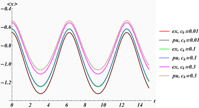
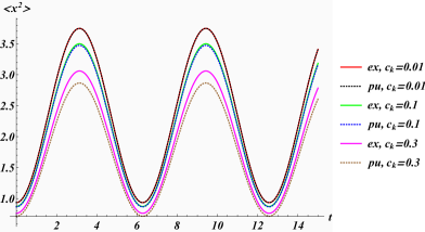
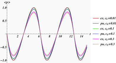
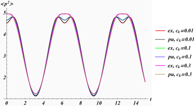
Figure 1: Exact versus perturbative expectation values for $x$, $x^{2}$, $p$, $p^{2}$ for $E_{0}=2$, $\omega=1/2$, $\tau=1$, $m=3$ and $n=1$ for different values of the expansion parameter $c_{k}$.

A further useful quantity to compute that illustrates the quality of the perturbative approach is the autocorrelation function

$$A_{n}(t):=\left|\left\langle\psi_{n}(t)\right.\left|\psi_{n}(0)\right\rangle\right|.$$ (62)

Unlike the expectation values for position, momenta and their squares the autocorrelation function also captures the influence of the time-dependent phase $\alpha(t)$. We depict this function in figure 2. In this case the overall agreement decreases for larger values of $n$.

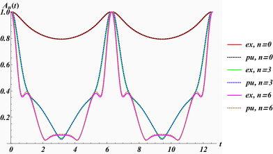
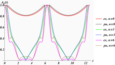
Figure 2: Exact versus perturbative autocorrelation function for $E_{0}=2$, $\omega=1/2$, $\tau=1$, $m=3$, different values for $n$ with $c_{k}=0.1$ in the left panel and $c_{k}=0.3$ in the right panel.

Next we compare directly the wave functions obtained three alternative ways. Figure 3 shows an extremely good agreement between the WKB approximation and the exact solution, except near the turning points $\xi_{\pm}$ where the WKB approximation is singular. The pertubative solution is in very good agreement with the exact solution for small values of $c_{\kappa}$, as expected. With increasing values of $c_{\kappa}$ the perturbative solution starts to deviate stronger in the negative regime for $\xi$ and large values of $n$.

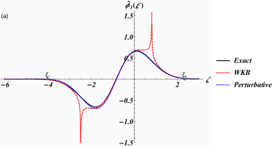
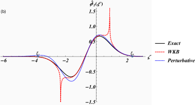
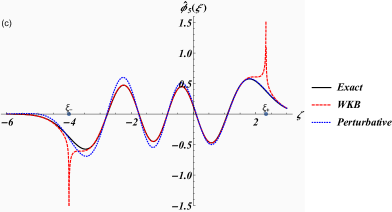
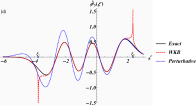
Figure 3: Exact versus WKB and perturbative solutions to the time-independent eigenvalue equation (3) for the invariant $\hat{I}$ with $\hbar=1$, $E_{0}=1$, $m=1$, $n=1$, $\tau=1$ and $c_{\kappa}=0.18$ in panels (a), (c), $c_{\kappa}=0.2$ in panels (b), (d). $\xi_{\pm}$ are the classical turning points (47).

Let us next see how these properties are inherited in the time-dependent system. Figure 4 displays the real part of the full time-dependent wave function. We observe the oscillation of the turning points with time that enter through the function $\sigma(t)$. As in the time-independent case, extremely good agreement between the WKB approximation and the exact solution, except near the turning points $x_{\pm}$. The perturbative solution slightly overshoots at the maxima and minima, especially in the negative time regime. The discrepancy becomes worse for larger values of $n$, which we do not show here.

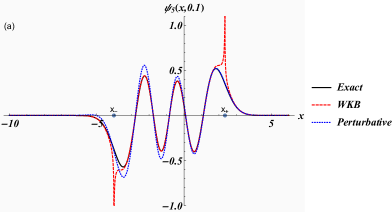
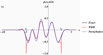
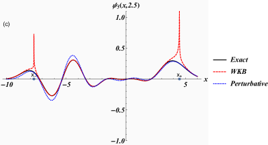
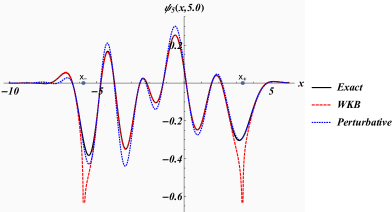
Figure 4: Exact versus WKB and perturbative solutions to the time-dependent Schrödinger equation (1) at different times with $\hbar=1$, $E_{0}=1$, $m=1$, $n=5$, $\tau=1$, $\omega=0.5$ and $c_{\kappa}=0.1$. The time-dependent classical turning points $\xi_{\pm}$ are indicated.

4 Goldman-Krivchenko potential with time-dependent perturbation

In trying to identify solvable systems we have seen in equation (25) that the value $p=-2$ is special as in that case the potential becomes the time-independent Goldman-Krivchenko potential [40], being a particular spiked harmonic oscillator [41, 42]. This potential may serve also as a benchmark for which we can solve the eigenvalue equation exactly and campare it to the perturbative solution. Hence we take this potential as our unperturbed system and perturb it by dropping the Stark term and replacing it by $x^{2}E(t)$. Thus we consider the time-dependent Hamiltonian

$$H(t)=\frac{p^{2}}{2m}+\frac{m\omega^{2}}{2}x^{2}+\frac{m\Omega^{2}}{2}\frac{1}{x^{2}}+x^{2}E(t).$$ (63)

It follows from above that the invariant for this system is

$$I(t)=\frac{1}{2}\left[\sigma^{2}p^{2}-m\sigma\dot{\sigma}\{x,p\}+\left(m^{2}\dot{\sigma}^{2}+\frac{\tau m^{2}+2mE_{0}}{\sigma^{2}}\right)x^{2}+m^{2}\sigma^{2}\Omega^{2}\frac{1}{x^{2}}\right],$$ (64)

with constraint $E(t)=E_{0}/\sigma^{4}$ and $\sigma$ satisfying the EP-equation (23). Also in this case we may complete the remaining steps in the Lewis-Riesenfeld approach and hence compare the exact and the perturbative solution. We identify $E_{0}\ll 1$ as the expansion parameter in the perturbative series.

4.1 Testing the approximate solution

4.1.1 Exact computation

Using the same similarity and variable transformation as in (34) we obtain the time-independent invariant

$$\hat{I}=UIU^{-1}=-\frac{1}{2}\partial_{\xi}^{2}+\frac{1}{2}\left(\tau m^{2}+2mE_{0}\right)\xi^{2}+\frac{m^{2}\Omega^{2}}{2}\frac{1}{\xi^{2}}.$$ (65)

We solve the eigenvalue equation $\hat{I}\Xi(\zeta)=\lambda\Xi(\zeta)$ exactly obtaining the solution

$$\Xi(\zeta)=\zeta^{(1+b/2)}e^{-\frac{a}{2}\zeta^{2}}\left[c_{1}L_{\nu_{-}}^{b/2}\left(a\zeta^{2}\right)+c_{2}U\left(\nu_{+},1+b/2,\frac{m\sqrt{\tau}\zeta^{2}}{\hbar}\right)\right],$$ (66)

where $L_{\nu}^{\mu}(z)$ denotes the generalized Laguerre polynomials, $U\left(\nu,\mu,z\right)$ the confluent hypergeometric function and $\nu_{\pm}:=\pm\left(2+b-2\lambda/a\right)/4$, $a=\sqrt{\tau m^{2}+2mE_{0}}$, $b:=\sqrt{1+4m^{2}\Omega^{2}}$. Demanding again that the eigenfunctions vanish asymptotically, i.e. $\lim_{\zeta\rightarrow\pm\infty}$ $\Xi(\zeta)=0$, imposes $\nu_{\pm}=n\in\mathbb{N}_{0}$ and thus quantizes $\lambda$. We discard the solution related to $U$, as its corresponding eigenvalues are not bounded from below, leading to the eigenfuctions and eigenvalues

$$\Xi_{n}(\zeta)=c_{1}\zeta^{(1+b/2)}e^{-\frac{a}{2}\zeta^{2}}L_{n}^{b/2}\left(a\zeta^{2}\right),\qquad\lambda_{n}=a(2n+1+b/2).$$ (67)

Assembling everything we obtain for the operator $I(t)$ the normalized eigenfunction from $U^{-1}\Xi_{n}(x/\sigma)$ as

$$\phi_{n}(x)=\sqrt{\frac{2n!}{[1-(-1)^{b}]\Gamma\left(1+n+b/2\right)}}\left(\frac{a}{\sigma^{2}}\right)^{(2+b)/4}x^{(1+b)/2}e^{-\frac{a}{2\sigma^{2}}x^{2}}L_{n}^{b/2}\left(\frac{ax^{2}}{\sigma^{2}}\right)e^{im\dot{\sigma}x^{2}/2\sigma\hbar}.$$ (68)

when $\mathop{\mathrm{R}e}b>-2$ and $\mathop{\mathrm{R}e}(a/\sigma^{2})>0$. This completes the second step in the Lewis-Riesenfeld approach. In the third and last step we determine the phase $\alpha$ by means of (5). The right hand side is computed once more to

$$\left\langle\phi_{n}\right|i\partial_{t}-H(t)\left|\phi_{n}\right\rangle=-\frac{\lambda_{n}}{m\sigma^{2}}$$ (69)

so that the phase acquires the same form as in the previous example

$$\alpha_{n}(t)=-\frac{1}{m\sqrt{\tau}}\lambda_{n}\arctan\left[\frac{\sqrt{\tau}\tan\left(\omega t\right)}{\omega}\right].$$ (70)

Let us now compare these expressions with those obtained in the perturbative computation.

4.1.2 Perturbative computation

We treat the term $V_{p}(x,t)=x^{2}E(t)$ with $E(t)=E_{0}/\sigma^{4}$ and $E_{0}\ll 1$ in the Hamiltonian as a perturbation. Accordingly we split up the invariant (33) as $I(t)=I_{0}(t)+E_{0}I_{p}(t)$ with

$$I_{0}(t)=\frac{1}{2}\left[\sigma^{2}p^{2}-m\sigma\dot{\sigma}\{x,p\}+\left(m^{2}\dot{\sigma}^{2}+\frac{\tau m^{2}}{\sigma^{2}}\right)x^{2}+m^{2}\sigma^{2}\Omega^{2}\frac{1}{x^{2}}\right],\quad~{}~{}I_{p}(t)=\frac{m}{\sigma^{2}}x^{2}.$$ (71)

The zeroth order wavefunction $\left|\phi_{n}^{(0)}\right\rangle$ is simply $\phi_{n}(x)$ in (68) with $E_{0}=0$. From (7) and (9) we compute first two terms in the perturbative series for the eigenvalues

$$\lambda_{n}^{(0)} = \left(2n+1+\sqrt{1+4m^{2}\Omega^{2}}/2\right)m\sqrt{\tau},\quad$$ (72)

$$\lambda_{n}^{(1)} = \left\langle\phi_{n}^{(0)}\right|I_{p}(t)\left|\phi_{n}^{(0)}\right\rangle=\left(2n+1\right)\sqrt{\frac{1+4m^{2}\Omega^{2}}{\tau}}.$$ (73)

As expected the eigenvalues are time-independent and $\lambda_{n}^{(0)}+E_{0}\lambda_{n}^{(1)}$ corresponds to (67) expanded to first order in $E_{0}$. Next we need to compute the infinite sum in (9) to determine the corrections to the wavefunctions. In this case there are only two terms contributing in the infinite sum. We compute

$$\left|\phi_{n}^{(1)}\right\rangle=\frac{1}{2m\tau}\left[\sqrt{(n+1)(n+1+b/2)}\left|\phi_{n+1}^{(0)}\right\rangle-\sqrt{n(n+b/2)}\left|\phi_{n-1}^{(0)}\right\rangle\right].$$ (74)

In the last step we compute the perturbed expression for the phase $\alpha_{n}^{(1)}(t)$ using equation (5). Once more we find up to first order

$$\alpha_{n}^{(1)}(t)=-\frac{\lambda_{n}^{(0)}+c_{\kappa}\lambda_{n}^{(1)}}{m\sqrt{\tau}}\arctan\left[\frac{\sqrt{\tau}\tan\left(\omega t\right)}{\omega}\right],$$ (75)

so that we have obtained the full perturbative solution to the TDSE as $\left|\psi_{n}\right\rangle^{(1)}$ as defined in (13).

4.1.3 Exact versus perturbative solutions

As previously, we compute several physical quantities to compare the exact and the perturbative solution. The momentum, position, squared momentum and squared position expectation values are computed to

$$\begin{array}[]{ll}\left\langle\psi_{n}\right|x\left|\psi_{n}\right\rangle=0,{}&\left\langle\psi_{n}\right|x^{2}\left|\psi_{n}\right\rangle=\frac{(2n+\ell+3/2)\sigma^{2}}{\sqrt{\tau m^{2}+2mE_{0}}},\\ \left\langle\psi_{n}\right|p\left|\psi_{n}\right\rangle=0,&\left\langle\psi_{n}\right|p^{2}\left|\psi_{n}\right\rangle=\frac{(4n+2)\ell+2n+3/2}{2\ell+1}\frac{\sqrt{\tau m^{2}+2mE_{0}}}{\sigma^{2}}+\frac{(2n+\ell+3/2)m\dot{\sigma}^{2}}{\sqrt{\tau m^{2}+2mE_{0}}}.\end{array}$$ (76)

In order to achieve convergence we had to impose the additional constraint $b=2\ell+1$ with $\ell\in\mathbb{N}_{0}$. The uncertainty relation becomes

$$\Delta x\Delta p=\sqrt{\frac{(2n+\ell+3/2)[(4n+2)\ell+2n+3/2]}{2\ell+1}+\frac{m(2n+\ell+3/2)^{2}\sigma^{2}\dot{\sigma}^{2}}{(\tau m+2E_{0})^{2}}},$$ (77)

with the lower bound $\Delta x\Delta p\geq 1/2$ always well respected.

Using the perturbed solutions (74) and (75) we compute

$$\begin{array}[]{l}\left\langle\psi_{n}\right|x\left|\psi_{n}\right\rangle^{(1)}=0,~{}~{}\left\langle\psi_{n}\right|x^{2}\left|\psi_{n}\right\rangle^{(1)}=(2n+\ell+3/2)(m\tau-E_{0})\frac{\sigma^{2}}{\tau m^{2}},\\ \left\langle\psi_{n}\right|p\left|\psi_{n}\right\rangle^{(1)}=0,~{}~{}\left\langle\psi_{n}\right|p^{2}\left|\psi_{n}\right\rangle^{(1)}=\frac{(4n+2)\ell+2n+3/2}{2\ell+1}\frac{(m\tau+E_{0})}{\sqrt{\tau}\sigma^{2}}+\frac{(2n+\ell+3/2)(\tau m-E_{0})\dot{\sigma}^{2}}{\tau^{3/2}}.\end{array}$$ (78)

The approximated uncertainty relation results to

$$\Delta x\Delta p^{(1)}=\sqrt{\frac{(2n+\ell+3/2)[(4n+2)\ell+2n+3/2]}{2\ell+1}(1-\frac{E_{0}^{2}}{m^{2}\tau^{2}})}.$$ (79)

We are now in the position to compare the exact and the pertubative solution. In figure 5 we compare the time-dependent expectation values for $x^{2}$ and $p^{2}$ computed in an exact way with those computed in a perturbative fashion. As in the previous example, the agreement is very good for small values of the expansion parameter, $E_{0}$ in this case. Overall the agreement is increasing for large values of $n$ as well as $m$ and for $\omega$ approaching $\sqrt{\tau}$.

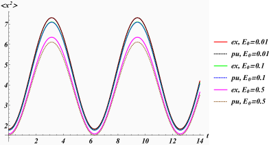
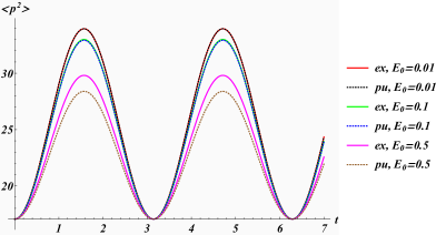
Figure 5: Exact versus perturbative expectation values for $x^{2}$, $p^{2}$, for $\omega=1/2$, $\tau=1$, $\ell=2$, $m=3$ and $n=1$ for different values of the expansion parameter $E_{0}$.

As in the previous example we also compute the autocorrelation function (62) as it captures well the effect from the time-dependent phase $\alpha(t)$. We depict this function in figure 6. Once more, the overall agreement decreases for larger values of $n$.

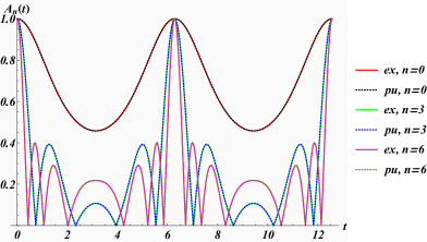
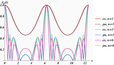
Figure 6: Exact versus perturbative autocorrelation function for $\omega=1/2$, $\tau=1$, $m=3$, $\ell=2$ and different values for $n$ with $E_{0}=0.1$ in the left panel and $E_{0}=0.5$ in the right panel.

5 Conclusions

We have explored the possibilty of a modified approximated Lewis and Riesenfeld method by solving the time-independent eigenvalue equation in the second step by means of standard time-independent perturbation theory. We have tested the quality of this approach for two classes of optical potentials by comparing the exact solutions obtained from the completely exact solution of the Lewis-Riesenfeld approach to the approximated ones, the perturbative approach and the WKB approximation. We computed some standard expectation values and the autocorrelation functions in two alternative ways. For the pertubative approach we found in general good agreement which is naturally improved in quality for smaller values of the expansion parameters. The WKB approximation is not limited to these small parameters and only deviates significantly at the turning points. Our semi-exactly solvable approach significantly widens the scope of the Lewis-Riesenfeld method and allows to tackle more complicated physical situations that are not possible to treat when insisting on full exact solvabilty

While in this paper we were mainly concerned with a proof of concept related to the modification of the Lewis-Riesenfeld method, it would naturally be very interesting now to apply the scheme to study more interesting and challenging physical phenomena. To this end one may carry out further approximations. Here we are still assuming that the first step in the approach, i.e. the computation of the invariant, can be carried out in an exact manner. Naturally one may also weaken this requirement and work with an approximated invariant in the second step. We will present this possibility elsewhere [43].

Acknowledgments: RT is supported by a City, University of London Research Fellowship. We thank Carla Figueira de Morisson Faria for discussions and comments.

References

- [1] A. Ashkin, Acceleration and trapping of particles by radiation pressure, Phys. Rev. Lett. 24(4), 156 (1970).
- [2] K. C. Neuman and S. M. Block, Optical trapping, Review of scientific instruments 75(9), 2787–2809 (2004).
- [3] A. Ashkin, J. M. Dziedzic, J. E. Bjorkholm, and S. Chu, Observation of a single-beam gradient force optical trap for dielectric particles, Optics Letters 11(5), 288–290 (1986).
- [4] H. J. Metcalf and P. Van der Straten, Laser cooling and trapping of neutral atoms, The Optics Encyclopedia: Basic Foundations and Practical Applications (2007).
- [5] A. D. Cronin, J. Schmiedmayer, and D. E. Pritchard, Optics and interferometry with atoms and molecules, Rev. of Mod. Phys. 81(3), 1051 (2009).
- [6] A. Ashkin, J. M. Dziedzic, and T. Yamane, Optical trapping and manipulation of single cells using infrared laser beams, Nature 330(6150), 769 (1987).
- [7] A. Ashkin and J. M. Dziedzic, Optical trapping and manipulation of viruses and bacteria, Science 235(4795), 1517–1520 (1987).
- [8] K. M. O’hara, M. E. Gehm, S. R. Granade, and J. E. Thomas, Scaling laws for evaporative cooling in time-dependent optical traps, Phys. Rev. A 64(5), 051403 (2001).
- [9] R. Fulton, A. I. Bishop, M. N. Shneider, and P. F. Barker, Controlling the motion of cold molecules with deep periodic optical potentials, Nature Physics 2(7), 465 (2006).
- [10] M. Born and V. Fock, Beweis des adiabatensatzes, Zeitschrift für Physik 51(3-4), 165–180 (1928).
- [11] K. Amini, J. Biegert, F. Calegari, A. Chacón, M. F. Ciappina, A. Dauphin, D. K. Efimov, C. Figueira de Morisson Faria, K. Giergiel, P. Gniewek, et al., Symphony on Strong Field Approximation, arXiv preprint arXiv:1812.11447 (2018).
- [12] A. Fring, V. Kostrykin, and R. Schrader, On the absence of bound-state stabilization through short ultra-intense fields, J. Phys. B29, 5651–567 (1996).
- [13] C. Figueira de Morisson Faria, A. Fring, and R. Schrader, Analytical treatment of stabilization, Laser Physics 9, 379–387 (1999).
- [14] C. Figueira de Morisson Faria, A. Fring, and R. Schrader, Existence criteria for stabilization from the scaling behaviour of ionization probabilities, J. Phys. B33, 1675–168 (2000).
- [15] L. Keldysh, Ionization in the field of a strong electromagnetic wave, Sov. Phys. JETP 20(5), 1307–1314 (1965).
- [16] F. H. M. Faisal, Multiple absorption of laser photons by atoms, J. of Phys. B: Atomic and Molecular Physics 6(4), L89 (1973).
- [17] H. R. Reiss, Effect of an intense electromagnetic field on a weakly bound system, Phys. Rev. A 22(5), 1786 (1980).
- [18] H. Lewis and W. Riesenfeld, An Exact quantum theory of the time dependent harmonic oscillator and of a charged particle time dependent electromagnetic field, J. Math. Phys. 10, 1458–1473 (1969).
- [19] I. A. Pedrosa, Exact wave functions of a harmonic oscillator with time-dependent mass and frequency, Phys. Rev. A 55(4), 3219 (1997).
- [20] M. S. Abdalla, Charged particle in the presence of a variable magnetic field, Phys. Rev. A 37(10), 4026 (1988).
- [21] Y. Bouguerra, M. Maamache, and A. Bounames, Time-dependent 2D harmonic oscillator in presence of the Aharanov-Bohm effect, Int. J. of Theor. Phys. 45(9), 1791–1797 (2006).
- [22] M. Maamache and H. Choutri, Exact evolution of the generalized damped harmonic oscillator, J. of Phys. A: Math. and Gen. 33(35), 6203 (2000).
- [23] S. Menouar, M. Maamache, Y. Saâdi, and J. R. Choi, Exact wavefunctions for a time-dependent Coulomb potential, J. of Phys. A: Math. and Theor. 41(21), 215303 (2008).
- [24] Y. Z. Lai, J. Q. Liang, H. J. W. Müller-Kirsten, and J. G. Zhou, Time-dependent quantum systems and the invariant Hermitian operator, Phys. Rev. A 53(5), 3691 (1996).
- [25] M. Maamache, Unitary transformation approach to the cyclic evolution of SU (1, 1) and SU (2) time-dependent systems and geometrical phases, J. of Phys. A: Math. and Gen. 31(32), 6849 (1998).
- [26] J. R. Choi and I. H. Nahm, SU (1, 1) Lie algebra applied to the general time-dependent quadratic Hamiltonian system, Int. J. of Theor. Phys. 46(1), 1–15 (2007).
- [27] X. Chen, E. Torrontegui, and J. G. Muga, Lewis-Riesenfeld invariants and transitionless quantum driving, Phys. Rev. A 83(6), 062116 (2011).
- [28] M.-A. Fasihi, Y. Wan, and M. Nakahara, Non-adiabatic Fast Control of Mixed States Based on Lewis–Riesenfeld Invariant, J. Phys. Soc. of Japan 81(2), 024007 (2012).
- [29] S. Dey and A. Fring, Noncommutative quantum mechanics in a time-dependent background, Phys. Rev. D 90, 084005 (2014).
- [30] A. Fring and T. Frith, Exact analytical solutions for time-dependent Hermitian Hamiltonian systems from static unobservable non-Hermitian Hamiltonians, Phys. Rev. A 95, 010102(R) (2017).
- [31] A. Fring and T. Frith, Solvable two-dimensional time-dependent non-Hermitian quantum systems with infinite dimensional Hilbert space in the broken PT-regime, J. of Phys. A: Math. and Theor. 51(26), 265301 (2018).
- [32] A. Fring and T. Frith, Quasi-exactly solvable quantum systems with explicitly time-dependent Hamiltonians, preprint arXiv:1808.03547 (2018).
- [33] J. Cen, A. Fring, and T. Frith, Time-dependent Darboux (supersymmetric) transformations for non-Hermitian quantum systems, J. of Phys. A: Math. and Theor. 52(11), 115302 (2019).
- [34] C. M. Bender and S. A. Orszag, Advanced mathematical methods for scientists and engineers I: Asymptotic methods and perturbation theory, Springer Science & Business Media, 2013.
- [35] V. Ermakov, Transformation of differential equations,, Univ. Izv. Kiev. 20, 1–19 (1880).
- [36] E. Pinney, The nonlinear differential equation , Proc. Amer. Math. Soc. 1, 681(1) (1950).
- [37] C. M. Bender and S. Boettcher, Real Spectra in Non-Hermitian Hamiltonians Having PT Symmetry, Phys. Rev. Lett. 80, 5243–5246 (1998).
- [38] A. Mostafazadeh, Pseudo-Hermitian Representation of Quantum Mechanics, Int. J. Geom. Meth. Mod. Phys. 7, 1191–1306 (2010).
- [39] C. M. Bender, P. E. Dorey, C. Dunning, A. Fring, D. W. Hook, H. F. Jones, S. Kuzhel, G. Levai, and R. Tateo, PT Symmetry: In Quantum and Classical Physics, (World Scientific, Singapore) (2019).
- [40] I. I. Goldman and V. D. Krivchenkov, Problems in quantum mechanics, (Pergamon Press, London 1961).
- [41] R. L. Hall, N. Saad, and A. B. von Keviczky, Generalized spiked harmonic oscillator, J. of Phys. A: Math. and Gen. 34(6), 1169 (2001).
- [42] M. Znojil, Spiked harmonic oscillator and Hill determinants, Phys. Lett. A 169(6), 415–421 (1992).
- [43] A. Fring and R. Tenney, in preparation.