Finding Needles in a Moving Haystack: Prioritizing Alerts with Adversarial Reinforcement Learning

Abstract

Detection of malicious behavior is a fundamental problem in security. One of the major challenges in using detection systems in practice is in dealing with an overwhelming number of alerts that are triggered by normal behavior (the so-called false positives), obscuring alerts resulting from actual malicious activity. While numerous methods for reducing the scope of this issue have been proposed, ultimately one must still decide how to prioritize which alerts to investigate, and most existing prioritization methods are heuristic, for example, based on suspiciousness or priority scores. We introduce a novel approach for computing a policy for prioritizing alerts using adversarial reinforcement learning. Our approach assumes that the attacker knows the full state of the detection system and the defender’s alert prioritization policy, and will dynamically choose an optimal attack. The first step of our approach is to capture the interaction between the defender and attacker in a game theoretic model. To tackle the computational complexity of solving this game to obtain a dynamic stochastic alert prioritization policy, we propose an adversarial reinforcement learning framework. In this framework, we use neural reinforcement learning to compute best response policies for both the defender and the adversary to an arbitrary stochastic policy of the other. We then use these in a double-oracle framework to obtain an approximate equilibrium of the game, which in turn yields a robust stochastic policy for the defender. Extensive experiments using case studies in fraud and intrusion detection demonstrate that our approach is effective in creating robust alert prioritization policies.

I Introduction

One of the core problems in security is detection of malicious behavior, with examples including detection of malicious software, emails, websites, and network traffic. There is a vast literature on detection approaches, ranging from signature-based to machine-learning based [8, 26, 34]. Despite best efforts, however, false positives are inevitable. Moreover, one cannot in general reduce the rate of false alarms without missing some real attacks as a result. Under the pressure of practical considerations such as liability and accountability, these systems are often configured to produce a large amount of alerts in order to be sufficiently sensitive to capture most attacks. As a consequence, cybersecurity professionals are routinely inundated with alerts, and must sift through these overwhelmingly uninteresting logs to identify alerts that should be prioritized for closer inspection.

A considerable literature has therefore emerged attempting to reduce the number of false alerts without significantly affecting the ability to detect malicious behavior [16, 30, 13]. Most of these attempt to add meta-reasoning on top of detection systems that capture broader system state, combining related alerts, escalating priority based on correlated observations, or using alert correlation to dismiss false alarms [38]. Nevertheless, despite significant advances, there are typically still vastly more alerts than time to investigate them. With this state of affairs, alert prioritization approaches have emerged, but rely predominantly on predefined heuristics, such as sorting alerts by suspiciousness score or by potential associated risk [2]. However, any policy that deterministically orders alerts potentially opens the door for determined attackers who can simply choose attacks that are rarely investigated, thereby evading detection.

Building on the observation of the fundamental tradeoff between false alert and attack detection rate, we propose a novel computational approach for robust alert prioritization to address the challenge. Our approach assumes a strong attacker who knows the full state of the detection environment including which alerts have been triggered, which have been investigated in the past, and even the defender’s policy. We also assumed that the adversary is capable of finding and utilizing a near optimal attack strategy against the defender policy based on his knowledge of the system and defending policy. To defend against such a strong attacker, we propose to compute the optimal stochastic dynamic defender policy that chooses the alerts to investigate as a function of the observable state, and that is robust to our threat model. At the core of our technical approach is a combination of game theory with adversarial reinforcement learning (ARL). Specifically, we model the problem of robust alert prioritization as a game in which the defender chooses its stochastic and dynamic policy for prioritizing alerts, while the attacker chooses which attacks to execute, also dynamically with full knowledge of the system state. Our computational approach first uses neural reinforcement learning to compute approximately optimal policies for either player in response to a fixed stochastic policy of their counterpart. It then uses these (approximate) best response oracles as a part of a double-oracle framework, which iterates two steps: 1) solve a game involving a restricted set of policies by both players, and 2) augment the policy sets by calling the best response oracle for each player. Note that our approach is completely orthogonal to methods for reducing the number of false positive alerts, such as alert correlation, and is meant to be used in combination with these, rather than as an alternative. In particular, we can first apply alert correlation to obtain a reduced set of alerts, and subsequently use our approach for selecting which alerts to investigate. Since alert correlation cannot be overly aggressive in order to ensure that we still capture actual attacks, the number of alerts often still significantly exceeds the investigation budget.

We evaluate our approach experimentally in two application domains: intrusion detection, where we use the Suricata open-source intrusion-detection system (IDS) with a network IDS dataset, and fraud detection, with a detector learned from data using machine learning. In both settings, we show that our approach is significantly more effective than alternatives with respect to our threat model. Furthermore, we demonstrate that our approach remains highly effective, and better than baseline alternatives in nearly all cases, even when certain assumptions of our threat model are violated.

II System Model

Figure 1: System model. The Attack Oracle computes the attacker’s policy for executing attacks, which is implemented by the Attack Generator and then triggers alerts observed by the Attack Detection Environment. The Defense Oracle computes the defender’s alert prioritization policy, which is implemented by the Alert Analyzer.

II-A Overview

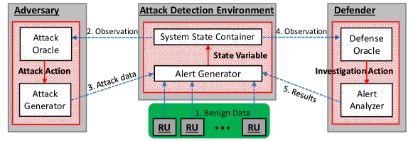
As displayed in Figure 1, our system is partitioned into four major components: a group of regular users (RU), an adversary (also called attacker), a defender, and an attack detection environment (ADE).

The regular users (RU) are the authorized users of a system. In contrast, the adversary is a sophisticated actor who attacks the target computer system. The attack detection environment (ADE) models the combination of the software artifact that is responsible for monitoring the system (e.g., network traffic, files, emails) and raising alerts for observed suspicious behavior, as well as relevant system state. System state includes attacks that have been executed (unknown to the defender), and alerts that have been investigated (known to both the attacker and defender). Crucially, the alerts triggered in the ADE may correspond either to behavior of the normal users RU, or to malicious behavior (attacks) by the adversary. We divide time into a series of discrete time periods. The defender is limited in how many alerts it can investigate in each time period and must select a small subset of alerts for investigation, while the adversary is limited in how many attacks it executes in each time period. The full system operates as follows for a representative time period (see again the schematic in Figure 1):

1. Benign alerts are generated by the ADE.

2. These alerts, and the remaining ADE system state (such as which alerts from past time periods have not yet been investigated, but could be investigated in the future), are observed by the attacker, who executes a collection of attacks.

3. The attacks trigger new alerts. These are arbitrarily mixed into the full collection of alerts, which is then observed by the defender.

4. The defender chooses a subset of alerts to investigate. The ADE state is updated accordingly, and the process repeats in the next time period.

Next, we describe our model of the alert detection environment, our threat model, and our defender model. The full list of notation that we use in the model is presented in Table I.

TABLE I: Notation summary.

Notation	Interpretation
Constants and functions
$A$	Types of attacks
$T$	Types of alerts
$C_{t}$	Cost of investigating an alert of type $t\in T$
$B$	Defender’s budget
$E_{a}$	Cost of mounting an attack of type $a\in A$
$D$	Adversary’s budget
$P_{a,t}(n)$	Probability that an attack $a\in A$ raises $n$ alerts of type $t\in T$
$\mathcal{F}_{t}$	Probability distribution of false alerts of type $t\in T$
$L_{a}$	Loss inflicted by an undetected attack $a\in A$
$\tau$	Temporal discounting factor
State variables (Time slot $k\in\mathbb{N}$)
$N_{t}^{(k)}$	Number of uninvestigated alerts of type $t\in T$
$M_{a}^{(k)}$	Indicator of whether an attack of type $a\in A$ was mounted
$S_{a,t}^{(k)}$	Number of alerts of type $t\in T$ raised due to attack $a\in A$
$R^{(k)}_{+1}$	Reward obtained by the defender
Actions, policies, and strategies
$\bm{\alpha}_{v}$	Action of player $v\in\{-1,+1\}$
$\bm{\pi}_{v}$	Policy (i.e., pure strategy) of player $v\in\{-1,+1\}$
$\bm{\sigma}_{v}$	Mixed strategy of player $v\in\{-1,+1\}$

II-B Attack Detection Environment (ADE) Model

Our model of the attack detection environment (ADE) captures a broad array of detection settings, including credit card fraud, intrusion, and malware detection. In this model, the ADE is composed of two parts: an alert generator (such as an intrusion detection system, like Suricata) and system state.

An alert generator produces a sequence of alerts in each time period. We aggregate alerts based on a finite predefined set of types $T$. For example, an alert type may be based on the application layer it was generated for (HTTP, DNS, etc), port number or range, destination IP address, and any other information that’s informative for determining the nature and relative priority of alerts. We can also define alert types for meaningful sequences of alerts. Indeed, the notion of alert types is entirely without loss of generality—we can define each type to be a unique sequence of alerts, for example—but in practice it is useful (indeed, crucial for scalability) to aggregate semantically similar alerts.

At the end of each time period the system generates a collection of alert counts for each alert type $t\in T$. We assume that normal or benign behavior generates alerts according to a known distribution $\mathcal{F}$, where $\mathcal{F}_{t}(n)$ is the marginal probability that $n$ alerts of type $t$ are generated. We also refer to this as the distribution of false alarms, since if the defender were omniscient, they would never trigger such alerts. Note that in practice it is not difficult to obtain the distribution $\mathcal{F}$. Specifically, we can use past logs of all alerts over some time period to learn the distribution $\mathcal{F}$. Since the vast majority of alerts in real systems are in fact false positives, any unidentified true positives in the logs will have a negligible impact.

We use three matrices to represent the state of ADE at time period $k$. The first represents the counts of alerts not yet investigated, grouped by type. Formally, we denote this structure by $\mathbf{N}^{(k)}=\{N_{t}^{(k)}\}_{t\in T}$, where $N_{t}^{(k)}$ is the number of alerts of type $t\in T$ that were raised but have not been investigated by the defender. This is observed by both the defender and the attacker. The second describes which attacks have been executed by the adversary; formally, $\mathbf{M}^{(k)}=\{M_{a}^{(k)}\}_{a\in A}$, where $M_{a}^{(k)}$ is a binary indicator where $M_{a}^{(k)}=1$ iff the attack $a$ was executed. This matrix is only observed by the attacker. Finally, we represent which alerts are raised specifically due to each attack. Formally, $\mathbf{S}^{(k)}=\{S_{a,t}^{(k)}\}_{a\in A,t\in T}$, where $S_{a,t}^{(k)}$ represents the number of alerts of type $t\in T$ raised due to attack $a$. This is also only observed by the attacker.

II-C Threat Model

Adversary’s Knowledge. We consider a strong attacker who is capable of observing the current state of the ADE. This obviates the need to make specific (and potentially erroneous) assumptions about information actually available to the attacker about system state; in practice, given the zero-sum nature of the encounter we consider below, having a less informed attacker will only improve the defender’s utility. Additionally, the attacker knows the randomized policy used by the defender for choosing which alerts to inspect (more on this below), and inspection decisions in previous rounds, but not the inspection decision in the current round (which happens after the attack).

Adversary’s Capabilities. In each time period, the adversary can execute multiple actions $a$ from a set of possible (representative) actions $A$. Each attack action $a\in A$ stochastically triggers alerts according to the probability distribution $P$, where $P_{a,t}(n)$ is the marginal probability that action $a$ generates $n$ alerts of type $t$. These probabilities can be learned by replaying known attack actions through actual detectors (as we do in the experiments below), ideally as a part of a full dataset which includes a mix of benign and malicious behavior. Commonly, alerts are generated deterministically for given attack actions; it is evident that our model admits this as a special case (i.e., $P_{a,t}\in\{0,1\}$). However, our generality allows us to handle important cases where alerts are, indeed, stochastic. For example, consider a Port Scan attack (as a part of a reconnaissance step). Port scan alert rules commonly consider the number of certain kinds of packets (such as ICMP packets) observed over a small time period (say, several seconds), and raise an alert if this number exceeds a predefined threshold. The number of such packets, of course, also depends on background traffic, which is stochastic, so that the triggering of the alert is also stochastic if the attack is sufficiently stealthy to avoid exceeding such a threshold in isolation.

Let $E_{a}$ be the cost for executing an attack $a\in A$. One method to estimate these costs is to examine the difficulty of executing the exploit based on the CVSS complexity metrics. The main limitation to the attacker capabilities is a budget constraint $D$ that limits how many, and which combination of, attacks can be executed. While it is difficult to reliably estimate this budget, our case studies in Section V demonstrate that our approach is robust to uncertainty about this parameter. Specifically, any attack decision $\bm{\alpha}_{-1}$ with $\alpha_{-1,a}$ the probability that the attack $a$ is executed by the attacker in a given time period, must abide by the following constraint:

$$\sum_{a\in A}\alpha_{-1,a}E_{a}\leq D.$$ (1)

For our purposes, it is useful to represent the attacker as consisting of two modules: Attack Oracle and Attack Generator, as seen in Figure 1. The attack oracle runs a policy, which maps observed the state of the ADE to attacks that are executed. In each time period, after observing ADE state, the attack oracle chooses attack actions, which are then executed by the attack generator, triggering alerts and thereby modifying the state of the ADE. Below we present our approach for approximating the optimal attack policies.

Adversary’s Goals. The adversary aims to successfully execute attacks. Success entails avoiding being detection by the defender, which only happens if alerts associated with an attack are inspected. Thus, if an attack triggers a collection of alerts, but none of these are chosen by the defender to be inspected in the current round, the attack succeeds. Different attacks, however, entail different consequences and, therefore, different rewards to the attacker (and loss to the defender). As a result, the adversary will ultimately need to balance rewards to be gained from successful attacks and the likelihood of being detected.

II-D Defender Model

Defender’s Knowledge. Unlike the adversary, the defender can only partially observe the state of the ADE. In particular, the defender only observes $\mathbf{N}^{(k)}$, the numbers of remaining uninvestigated alerts, grouped by alert type (since clearly the defender cannot directly observe actually attacks). In addition, we assume that the defender knows the attack budget and costs of (representative) attacks. In our experiments, we study the impact of relaxing this assumption (see Sections V-C5 and V-B5), and provide practical guidance on this issue.

Defender’s Capabilities. The defender chooses subsets of alerts in $\mathbf{N}^{(k)}$ to investigate in each time period $k$. This choice is constrained by the defender’s budget, which in practice can translate to time the defender has to investigate alerts. Since different types of alerts may need different amounts of time to investigate, or more generally, incur varying investigation costs, the budget constraint is on the total cost of investigating chosen alerts. Formally, let $C_{t}$ be the investigation cost of an alert of type $t$, and let $\alpha_{+1,t}^{(k)}$ be the number of alerts of type $t$ chosen to be investigated by the defender in period $k$. Then the budget constraint takes the following mathematical form:

$$\sum_{t\in T}C_{t}\alpha_{+1,t}^{(k)}\leq B.$$ (2)

An additional constraint imposed by the problem definition is that the defender can only investigate existing alerts:

$$\forall t\in T:\alpha_{+1,t}^{(k)}\leq N_{t}^{(k)}.$$ (3)

Just as with the adversary, it is useful to represent the defender as consisting of two modules: Defense Oracle and Alert Analyzer, as shown in Figure 1. The defense oracle runs a policy, which maps partially observed state of the ADE to the choice of a subset of alerts to be investigated. In each time period, after observing the set of as yet uninvestigated alerts, the defense oracle chooses which alerts to investigate, and this policy is then implemented by the alert analyzer, which thereby modifies ADE state (marking the selected alerts as having been investigated). Below we present our approach for approximately computing optimal defense policies that are robust to attacks as defined in our threat model above.

Defender’s Goals. The goal of the defender is to guard a computer system or network by detecting attacks through alert inspection. To achieve its goal, the defender develops an investigation policy to allocate its limited budget to investigation activities in order to minimize consequences of successful attacks, where we assume that an attack will fail to accomplish its primary objectives if the alerts it causes the ADE to emit are investigated in a timely manner.

II-E An Illustrative Example

Since our system is built on top of an abstracted model of alert investigation, the results are generally applicable to a wide range of real-world problems. We will use intrusion detection as an illustrative example in this section. Port Scan reconnaissance attack is one of the most common initial steps in remote exploitation and is a common occurrence faced by many enterprise IT professionals. In a Suricata IDS system, each alert item has different levels of categorization. For example, at the lowest layer, the port scan may trigger two types of alert, 1) Httprecon Web Server Fingerprint Scan, and 2) ET SCAN NMAP -sO. At a higher level, these alerts can be categorized into attempted-recon (since both reflect potential reconnaissance efforts by the attacker), as is the case in the Emerging Threats Ruleset of Suricata. A defender can choose different granularities of attack categorization to map the IDS alert types into the abstracted types in our proposed model based on individual needs. Besides categorization, the defender can also make use of other attributes in the IDS alerts to aid in abstracted type assignment. For example, a port scan on the enterprise file server can be assigned to the abstracted type of high-risk-recon, while a port scan on employee desktop can be assigned to attempted-recon.

In addition to the alerts corresponding to an actual attack action, normal user behavior can generate false positive alerts. For example, a user who is scraping the web for weather data monitoring may trigger the ET POLICY POSSIBLE Web Crawl using Curl, which is grouped into the attempted-recon type by the same Emerging Threats Suricata ruleset. Leveraging the proposed game-theoretic model on these abstracted alerts, it is possible for the defender to devise an optimal defense policy for a wide range of alert applications even in the face of possible false positives.

III Game Theoretic Model of
Robust Alert Prioritization

We now turn to the proposed approach for robust alert prioritization. We model the interaction between the defender and attacker as a zero-sum game, which allows us to define and subsequently compute robust stochastic inspection policies for the defender. In this section, we formally describe the game model. We then present the computational approach for solving it in Section IV.

The game has two players: the defender (denoted by $v=+1$) and the adversary (denoted by $v=-1$). Each player’s strategies are policies, that is, mappings from an observed ADE state to the probability distribution over actions to take in that state. In a given state, the defender chooses a subset of alerts to investigate; thus, the defender’s set of possible actions is the set of all alert subsets that satisfy the constraints (2) and (3). The attacker’s choices in a given state correspond to subsets of actions $A$ to take. Consequently, the set of adversary’s actions is the set of all subsets of attacks satisfying constraint (1). Note that the combinatorial nature of both players’ action spaces and of the state space makes even representing deterministic policies non-trivial; we will deal with this issue in Section IV. Moreover, we will consider stochastic policies. An equivalent way to represent stochastic policies is as probability distributions over deterministic policies, which map observed state to a particular action (subset of alerts for the defender, subset of attacks for the adversary). Henceforth, we call deterministic policies of the players their pure strategies and stochastic policies are termed mixed strategies, following standard terminology in game theory.

Let $\bm{\pi}_{-1}$ denote the attacker’s policy, which maps the fully observed state of ADE, $\bm{O}_{-1}^{(k)}=\langle\mathbf{N}^{(k)},\mathbf{M}^{(k)},\mathbf{S}^{(k)}\rangle$, to a subset of attacks. Let $\bm{\alpha}_{-1}^{(k)}=\bm{\pi}_{-1}(\bm{O}_{-1}^{(k)})$, where $\bm{\alpha}_{-1}^{(k)}=\{\alpha_{-1,a}^{(k)}\}_{a\in A}$ are (for the moment) binary indicators with $\alpha_{-1,a}^{(k)}=1$ iff an action $a\in A$ is chosen by the attacker. In other words, the vector $\bm{\alpha}_{-1}^{(k)}$ represents the choice of actions made by the adversary. Similarly, $\bm{\pi}_{+1}$ denotes the defender’s policy, which maps the portion of ADE state $\bm{O}_{+1}^{(k)}=\mathbf{N}^{(k)}$ observed by the defender to the number of alerts of each type to investigate. Aalogous to the attacker, $\bm{\alpha}_{+1}^{(k)}=\bm{\pi}_{+1}(\bm{O}_{+1}^{(k)})$, where $\bm{\alpha}_{+1}^{(k)}=\{\alpha_{+1,t}^{(k)}\}_{t\in T}$ are the counts of alerts chosen to be investigated for each type $t$. Now, notice that all alerts of type $t$ are equivalent by definition; consequently, it makes no difference to the defender which of these are chosen, and we therefore choose the fraction $\frac{\alpha_{+1,t}^{(k)}}{N_{t}^{(k)}}$ of alerts of type $t$ uniformly at random.

Let $\bm{\Pi}_{v}$ be player $v$’s set of pure strategies, where each pure strategy $\bm{\pi}_{v}\in\bm{\Pi}_{v}$ is a policy as defined above. A mixed strategy of player $v$ is then a probability distribution $\bm{\sigma}_{v}=\{\sigma_{v}(\bm{\pi}_{v})\}_{\bm{\pi}_{v}\in\bm{\Pi}_{v}}$ over the player’s pure strategies $\bm{\Pi}_{v}$ where $\sigma_{v}(\bm{\pi}_{v})$ is the probability that player $v$ uses policy $\bm{\pi}_{v}$. Since a mixed strategy $\bm{\sigma}_{v}$ is a distribution over a finite set of pure strategies, it satisfies $0\leq\sigma_{v}(\bm{\pi}_{v})\leq 1$ and $\sum_{\bm{\pi}_{v}\in\bm{\Pi}_{v}}\sigma_{v}(\bm{\pi}_{v})=1$. Let $\bm{\Sigma}_{v}$ denote the set of all mixed strategies of player $v$.

For any strategy profile of the two players, $(\bm{\pi}_{v},\bm{\pi}_{-v})$, we denote the utility of each player $v$ by $U_{v}(\bm{\pi}_{v},\bm{\pi}_{-v})$, $v\in\{+1,-1\}$. Since our game is zero-sum, $\sum_{v\in\{+1,-1\}}U_{v}(\bm{\pi}_{v},\bm{\pi}_{-v})=0$. When player $v$ chooses pure strategy $\bm{\pi}_{v}\in\bm{\Pi}_{v}$ and its opponent $-v$ plays mixed strategy $\bm{\sigma}_{-v}\in\bm{\Sigma}_{-v}$, then the expected utility of $v$ is

$$U_{v}(\bm{\pi}_{v},\bm{\sigma}_{-v})=\sum_{\bm{\pi}_{-v}\in\bm{\Pi}_{-v}}\sigma_{-v}(\bm{\pi}_{-v})U_{v}(\bm{\pi}_{v},\bm{\pi}_{-v}).$$ (4)

Similarly, the expected utility of player $v$ when it chooses the mixed strategy $\bm{\sigma}_{v}\in\bm{\Sigma}_{v}$ and its opponent play the mixed strategy $\bm{\sigma}_{-v}\in\bm{\Sigma}_{-v}$ is

$$U_{v}(\bm{\sigma}_{v},\bm{\sigma}_{-v})=\sum_{\bm{\pi}_{v}\in\bm{\Pi}_{v}}\sigma_{-v}(\bm{\pi}_{v})U_{v}(\bm{\pi}_{v},\bm{\sigma}_{-v}).$$ (5)

Next, we describe how to compute the utility of player $v$, $U_{v}(\bm{\pi}_{v},\bm{\pi}_{-v})$, when its policy is $\bm{\pi}_{v}$ and the opponent’s policy $\bm{\pi}_{-v}$ are given.

Consider arbitrary pure strategies of both players, $\bm{\pi}_{+1}$ and $\bm{\pi}_{-1}$. The game begins with an initial system state $\langle\bm{N}^{(0)},\bm{M}^{(0)},\bm{S}^{(0)}\rangle=\langle\bm{0},\bm{0},\bm{0}\rangle$. The system state is then updated in each time period $k$ as follows:

1. Alert investigation. The defender first investigates a subset of alerts produced thus far. Specifically, the defender chooses the number of alerts of each type to investigate $\{\alpha_{+1,t}^{(k)}\}_{t\in T}$ according to its policy $\bm{\pi}_{+1}(\bm{O}_{+1}^{(k)})$ given current observed state $\bm{O}_{+1}^{(k)}$. For each attack $a\in A$, let $\widetilde{M}_{a}^{(k)}$ be an indicator of whether attack $a$ has been executed by the beginning of time period $k$, but has not been investigated. If $M_{a}^{(k)}=0$, we have $\widetilde{M}_{a}^{(k)}=0$ as no attack $a\in A$ has been executed. If $M_{a}^{(k)}=1$, then $\widetilde{M}_{a}^{(k)}=1$ with probability

   $$p_{a}^{(k)}=\prod_{t\in T}\left\{\frac{C(N^{(k)}_{t}-S^{(k)}_{a,t},\alpha_{+1,t}^{(k)})}{C(N^{(k)}_{t},\alpha_{+1,t}^{(k)})}\right\},$$ (6)

   where $C(n,r)$ is the number of possible combinations of $r$ objects from a set of $n$ objects. $p_{a}^{(k)}$ is then the probability that attack $a$ is not detected by the defender.

2. Attack generation. The adversary produces attacks by executing actions according to its policy $\{\alpha_{-1,a}^{(k)}\}_{a\in A}=\bm{\pi}_{-1}(\bm{O}_{-1}^{(k)})$ given the fully observed ADE state $\bm{O}_{-1}^{(k)}$. Then $M_{a}^{(k+1)}=\alpha_{-1,a}^{(k)}$ for each $a\in A$.

3. Triggering alerts. Each attack $a\in A$ can trigger alerts as follows. For each attack $a\in A$ and alert type $t\in T$, if $M_{a}^{(k+1)}=1$, then $S_{a,t}^{(k+1)}=n$ with probability $P_{a,t}(n)$ for $n\geq 0$. This probability can be estimated, for example, by feeding inputs which include representative attacks into an attack detector and observing relative frequencies of alerts that are triggered. In addition, false alerts are generated according to the distribution $\mathcal{F}_{t}$, which we can estimate from data of normal behavior and associated alert counts. Let $f_{t}^{(k)}$ be the number of false alerts of type $t\in T$ that have been generated. Then the total number of alerts in the next time period $k+1$ is $N_{t}^{(k+1)}=f_{t}^{(k)}+S_{a,t}^{(k+1)}$.

In order to define the reward received by the defender in time period $k$, we make the following assumption: if any of the alerts raised by an attack is chosen to be inspected, then the attack is detected; otherwise, the attack is not detected. Let $L_{a}$ be the loss incurred by the defender when an attack $a\in A$ is not detected. Then the reward of the defender obtained in time period $k$ is

$$R_{+1}^{(k)}=-\sum_{a\in A}L_{a}\cdot\widetilde{M}_{a}^{(k)}.$$ (7)

For an arbitrary pure strategy profile of the defender and adversary, $(\bm{\pi}_{+1},\bm{\pi}_{-1})$, the defender’s utility from the game is the expected total discounted sum of the reward accrued in each time period:

$$U_{+1}(\bm{\pi}_{+1},\bm{\pi}_{-1})=\mathbb{E}\left[\sum_{k=0}^{\infty}\tau^{k}\cdot R_{+1}^{(k)}\right],$$ (8)

where $\tau\in(0,1)$ is a temporal discounting factor which implies that future rewards are less important than current rewards. That is, imminent losses are more important to the defender than potential future losses. The adversary’s utility is then $U_{-1}(\bm{\pi}_{+1},\bm{\pi}_{-1})=-U_{+1}(\bm{\pi}_{+1},\bm{\pi}_{-1})$.

Our goal of finding robust alert investigation policies amounts to computing a mixed-strategy Nash equilibrium (MSNE) of our game by the well-known equivalence between MSNE, maximin, and minimax solutions in zero-sum games [17]. A mixed-strategy profile $(\bm{\sigma}_{v}^{*},\bm{\sigma}_{-v}^{*})$ of the two players is an MSNE if it satisfies the following condition for all $v\in\{+1,-1\}$

$$U_{v}(\bm{\sigma}_{v}^{*},\bm{\sigma}_{-v}^{*})\geq U_{v}(\bm{\sigma}_{v},\bm{\sigma}_{-v}^{*})~{}~{}\forall\bm{\sigma}_{v}\in\bm{\Sigma}_{v}.$$ (9)

That is, each player $v$ chooses a stochastic policy $\bm{\sigma}_{v}^{*}$ that is the best response (is optimal for $v$) when its opponent chooses $\bm{\sigma}_{-v}^{*}$.

IV Computing Robust Alert
Prioritization Policies

Figure 2: The game solver based on the double oracle algorithm.

IV-A Solution Overview

For given sets of policies, $\bm{\Pi}_{+1}$ and $\bm{\Pi}_{-1}$, a standard approach to computing the MSNE of a zero-sum game is to solve a linear program of the following form:

$$\begin{array}[]{ll@{}ll}\text{max}&U_{v}^{*}&\\ \text{s.t.}&\sum_{\bm{\pi}_{v}\in\bm{\Pi}_{v}}U_{v}(\bm{\pi}_{v},\bm{\pi}_{-v})\cdot\sigma_{v}(\bm{\pi}_{v})\geq U_{v}^{*},{}&\forall\bm{\pi}_{-v}\in\bm{\Pi}_{-v}\\ &\sum_{\bm{\pi}_{v}\in\bm{\Pi}_{v}}\sigma_{v}(\bm{\pi}_{v})=1&\\ &\displaystyle\sigma_{v}(\bm{\pi}_{v})\geq 0&\forall\bm{\pi}_{v}\in\bm{\Pi}_{v}\end{array}$$ (10)

where in our case the optimal solution $\bm{\sigma}_{+1}^{*}$ yields the robust alert prioritization policy for the defender. However, using this approach for our problem entails two principal technical challenges: 1) the space of policies for both players is intractably large, and 2) it is even intractable to explicitly represent individual policies, since they map a combinatorial set of states to a combinatorial set of actions for both players.

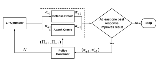
We propose an adversarial reinforcement learning approach to address these challenges, which combines a double oracle framework [25] with neural reinforcement learning. The general double oracle approach is illustrated in Figure 2. We start with an arbitrary small collection of policies for both players, $(\bm{\Pi}_{+1},\bm{\Pi}_{-1})$, and solve the linear program (10), obtaining provisional equilibrium mixed strategies $(\bm{\sigma}_{+1},\bm{\sigma}_{-1})$ of the restricted game. Next, we query the attack oracle to compute the adversary’s best response $\bm{\pi}_{-1}(\bm{\sigma}_{+1})$ to the defender’s equilibrium mixed strategy $\bm{\sigma}_{+1}$, and, similarly, query the defense oracle to compute the defender’s best response $\bm{\pi}_{+1}(\bm{\sigma}_{-1})$ to the adversary’s equilibrium mixed strategy $\bm{\sigma}_{-1}$. The best response policies are then added to the policy sets $(\bm{\Pi}_{+1},\bm{\Pi}_{-1})$ of the players, and we then re-solve the linear program and repeat the process. The process stops when neither player’s best response policy yields appreciable improvement in utility compared to the provisional equilibrium mixed strategy. Since the space of possible policies in our case is infinite, this process may not converge. However, in our experiments the procedure converged in fewer than 15 iterations (see Figure 12 in Appendix -B), with the fast convergence in part due to the way we represent policies, as discussed below. The main question that remains is how to compute or approximate the best response oracles for both players. To this end, we use reinforcement learning techniques with policies represented using neural networks. Below, we explain both our double oracle approach and our neural reinforcement learning methods (including the specific way in which we represent policies) in further detail.

IV-B Policy-based Double Oracle Method

As displayed in Figure 2, our game solver is an extension of the double oracle algorithm proposed in [36] and is partitioned into four parts: a policy container, a linear programming (LP) optimizer, a defense oracle, and an attack oracle. The policy container stores the policies of the two players, $\bm{\Pi}_{+1}$ and $\bm{\Pi}_{-1}$, as well as a utility matrix $\bm{U}$, whose elements are $U_{+1}(\bm{\pi}_{+1},\bm{\pi}_{-1})$ for all $\bm{\pi}_{+1}\in\bm{\Pi}_{+1}$ and $\bm{\pi}_{-1}\in\bm{\Pi}_{-1}$. The LP optimizer solves the game by computing the current mixed-strategy Nash equilibrium given the utility matrix $\bm{U}$. The defense and attack oracles are agents that apply reinforcement learning to compute the optimal responses to their opponents’ mixed strategies, which are provided by the LP optimizer.

Our solver works in an iterative manner such that the players’ policies and the utility matrix grow incrementally. Initially, $\bm{\Pi}_{+1}$, $\bm{\Pi}_{-1}$ can be set up with some basic policies, for example, uniformly allocating each player’s budget among their choices. Then, the policy sets, jointly encapsulated in a policy container, are updated in each iteration as follows:

1. First, the LP optimizer computes the mixed-strategy Nash Equilibrium $(\bm{\sigma}_{+1}^{{}^{\prime}},\bm{\sigma}_{-1}^{{}^{\prime}})$ of the current iteration by solving the optimization problems presented in Equation (10).

2. The oracle of player $v$ computes the best response policy $\bm{\pi}^{\prime}_{v}$ given that its opponent uses its equilibrium mixed-strategy $\bm{\sigma}^{\prime}_{-v}$, for $v\in\{+1,-1\}$.

3. If $U_{v}(\bm{\pi}^{\prime}_{v},\bm{\sigma}^{\prime}_{-v})\leq U_{v}(\bm{\sigma}^{\prime}_{v},\bm{\sigma}^{\prime}_{-v})$ for all $v\in\{+1,-1\}$, the double oracle algorithm terminates and returns $(\bm{\sigma}^{\prime}_{+1},\bm{\sigma}^{\prime}_{-1})$ as the approximate MSNE. Otherwise, add $\bm{\pi}^{\prime}_{v}$ to the corresponding $\bm{\Pi}_{v}$, update the utility matrix $\bm{U}$ and continue from Step 2.

The resulting $(\bm{\sigma}_{+1}^{{}^{\prime}},\bm{\sigma}_{-1}^{{}^{\prime}})$ is an approximate mixed-strategy Nash equilibrium $(\bm{\sigma}_{+1}^{*},\bm{\sigma}_{-1}^{*})$.

Next, we describe how the defense and attack oracles apply neural reinforcement learning to compute their best responses to an arbitrary mixed-strategy of the opponent.

IV-C Approximate Best Response Oracles with Neural Reinforcement Learning

We now turn to our approach to compute $\bm{\pi}^{\prime}_{v}$, the optimal response of player $v$ when its opponent uses a mixed strategy $\bm{\sigma}^{\prime}_{-v}$ such that

$$\bm{\pi}^{\prime}_{v}=\operatorname*{arg\,max}_{\bm{\pi}_{v}}U_{v}(\bm{\pi}_{v},\bm{\sigma}^{\prime}_{-v}).$$ (11)

This problem poses a major technical challenge, since the spaces of possible policies for both the defender and the attacker are quite large. To address this, we propose using the reinforcement learning (RL) paradigm. However, the use of RL poses two further challenges in our setting. First, for a given state, each player’s set of possible actions is combinatorial. For example, the attacker is choosing subsets of attacks, whereas the defender is choosing subsets of alerts. Consequently, we cannot use common methods such as Q-learning, which requires explicitly representing the action-value function $Q(x,a)$ for every possible action $a$, even if we approximate this function over states $x$ using, e.g., a neural network, as is common in deep RL. We can address this issue by appealing to actor-critic methods for RL, where the policy is represented as a parametric function $\bm{\pi}_{v;\theta}$ with parameters $\theta$. However, this brings up the second challenge: actor-critic approaches learn policies using gradient-based methods, which require that the actions are continuous. In our case, however, the actions are discrete.

One solution is to learn the action-value function $Q(x,a)$ over a vector-based representation of actions, such as using a binary vector to indicate which attacks are used. The problem with this approach, however, is that the resulting policy $\bm{\pi}_{v}\in\arg\max_{a\in A}Q(x,a)$ is hard to compute in real time, since it involves a combinatorial optimization problem in its own right. We therefore opt for a much more scalable solution that uses the actor-critic paradigm with an alternative representation of the adversary and defender policies, which admits gradient-based learning.

Let us start with the adversary. Recall that the adversary’s policy maps a state to a subset of attack actions $A$, with the constraint on the total budget used by the chosen actions. Instead of returning a discrete subset of actions, we map the adversary’s policy to a probability distribution over actions, overloading our prior notation so that $\alpha_{-1,a}^{(k)}$ now denotes the probability that action $a\in A$ is executed. Now the policy can be used with actor-critic methods, but it may violate the budget constraint. To address this final issue, we simply project the probability distribution into the feasible space at execution time by normalizing it by the total cost of the distribution, and then multiplying by the budget constraint. Notice that in this process we have relaxed the attacker’s budget constraint to hold only in expectation; however, this only makes the attacker stronger. An interesting side-effect of our transformation of the adversary’s policy space is that the RL method will now effectively search in the space of stochastic adversary policies. An associated benefit is that it leads to faster convergence of the double oracle approach.

Next, consider the defender. In this case, we can simply represent the policy as a mapping to fractions of the total defense budget allocated to each alert type $t$. In other words, for each alert type $t$, the policy will output the maximum fraction of the defense budget that will be used to inspect alerts of type $t$. This simultaneously makes the mapping continuous, and obviates the need to explicitly deal with the budget constraint.

The final nuance is that RL methods are typically designed for a fixed environment, whereas our setting is a game. However, note that since we are concerned only with each player’s best response to the other’s mixed strategy, we can embed the mixed strategy of the opponent as a part of the environment. Next, we describe our application of actor-critic methods to our problem, given the alternative representations of adversary and defender policies above.

Figure 3: The interactions among actor, critic and environment.

The basic idea of the actor-critic method is that we can iteratively learn and improve a policy without enumerating actions by using two parallel processes that interact with each other: an actor which develops a policy, and a critic network which evaluates the policy. The interaction between the actor and critic in illustrated in Figure 3. In each iteration, the actor and critic proceed as follows:

1. The actor executes an action according to its policy given the observation of the environment.

2. Upon receiving the action, the environment updates its system state and returns a reward to the critic.

3. The critic updates its evaluation method and provides feedback to the actor.

4. The actor updates its policy according to the feedback given by the critic.

We propose DDPG-MIX, actor-critic algorithm that operates in continuous action spaces and computes an approximate best response to an opponent who uses a stochastic policy. DDPG-MIX is an extension of the Deep Deterministic Policy Gradient (DDPG) approach proposed in [20] to our setting, and the full algorithm is outlined in Algorithm 1 in the Appendix. For each player $v$, DDPG-MIX employs two neural networks to represent the actor and critic: a policy network $\bm{\pi}_{v}(\bm{O}_{v}|\bm{\theta}_{v}^{\pi})$ for the actor, which has parameters $\bm{\theta}_{v}^{\pi}$ and maps an observation $\bm{O}_{v}$ into an action, and a value network $Q_{v}(\bm{O}_{v},\bm{\alpha}_{v}|\bm{\theta}_{v}^{Q})$ for the critic, which has parameters $\bm{\theta}_{v}^{Q}$ and maps an observation $\bm{O}_{v}$ and an action $\bm{\alpha}_{v}$ into a value. Initially, these two neural networks are randomly initialized. Then, we train these two iteratively with multiple episodes, each of which contains multiple steps. At the beginning of each episode, the opponent samples a deterministic policy $\bm{\pi}_{-v}$ with its mixed-strategy $\bm{\sigma}_{-v}$. The policy network and value network are then updated as follows. First, we generate an action by using the $\epsilon$-greedy method: we randomly choose an action with probability $\epsilon$ (called exploration in RL), and apply the policy network $\bm{\pi}_{v}(\bm{O}_{v}|\bm{\theta}_{v}^{\pi})$ to produce an action corresponding to the current state with probability $1-\epsilon$ (called exploitation). Player $v$ then executes the action produced and so does its opponent, which executes an action $\bm{\alpha}_{-v}$ returned by $\bm{\pi}_{-v}$. Once the system state of the environment is updated, player $v$ receives the reward and stores the transition into a memory buffer. Player $v$ then samples a minibatch, a subset of transitions randomly sampled from the buffer, to update the value network $Q_{v}(\bm{O}_{v},\bm{\alpha}_{v}|\bm{\theta}_{v}^{Q})$ by minimizing a loss function as in most regression tasks. The sampled gradient of the value network with respect to $\bm{\alpha}_{v}$ is then forwarded to the policy network, which is further applied to update $\bm{\pi}_{v}(\bm{O}_{v}|\bm{\theta}_{v}^{\pi})$ as presented in Equation (12) in Algorithm 1. After a fixed number of episodes, the resulting policy network $\bm{\pi}_{v}(\bm{O}_{v}|\bm{\theta}_{v}^{\pi})$ is returned as the parameterized optimal response to an opponent with mixed-strategy $\bm{\sigma}_{-v}$.

IV-D Preprocessing

An important consideration in applying the above approaches is scalability of training. One way to significantly improve scalability is through preprocessing, and pruning alerts for which the (near-)optimal decision is obvious. We use the following pruning step to this end. Suppose that there is an alert type $t$ which is generated by benign traffic with probability at most $\epsilon$, where $\epsilon$ is very small (for example, $\epsilon=0$, in which case alerts of type $t$ never correspond to a false positive). In most realistic cases, it is nearly optimal to always inspect such alerts. Consequently, we prune all alerts with false positive rate below a small pre-defined $\epsilon$ (in our implementation below, we set $\epsilon=0$), and mark them for inspection (correspondingly reducing the available budget for inspecting other alerts).

V Case studies

In this section, we present case studies to investigate the robustness of our proposed approach for alert prioritization. We conduct our experiments in two applications: intrusion detection which employs a signature-based detection system and fraud detection which applies a learning-based detection system. We start with a broad introduction of the experimental methodology, including the details of the implementation of our approach and evaluation methods. We then proceed to describe each case study in detail.

V-A Experimental Methodology

V-A1 Implementation

TABLE II: Architecture of the implemented policy and value networks.

Neural network	Layer	Number of units	Activation function	Initializer
Policy network	Input	$T$ (defender); $|T|+|A|\cdot(1+|T|)$ (adversary)	-	-
	Hidden	16 (Fraud detection); 32 (Intrusion detection)	Tanh	Xavier [10]
	Output	$|T|$ (defender); $|A|$ (adversary)	Sigmoid	Xavier
Value netwrok	Input	$2\cdot|T|$ (defender); $|T|+|A|\cdot(2+|T|)$ (adversary)	-	-
	Hidden	32 (Fraud detection); 64 (Intrusion detection)	Relu	He Normal [11]
	Output	1	Relu	He Normal

The DDPG-MIX algorithm was implemented in TensorFlow [1], an open-source library for neural network learning. The architecture of the policy and value networks for both players are displayed in Table II. We used Adam for learning the parameters of the neural networks with learning rates of 0.001 and 0.002 for the policy and value networks, respectively. The discount factor $\tau$ was set to be 0.95, and we set the size of the memory buffer to 40,000. The learning process contained 500 episodes, each with 400 learning steps. The collection of policies used in the double-oracle framework was initialized with a pair of policies that uniformly allocate each player’s budget among their choices.

Our experiments were conducted on a server running Ubuntu 16.04 with Intel(R) Xeon(R) CPU E5-2695 v4 @ 2.10GHz, 18 cores and 64 GB memory. Each experiment was repeatedly executed 20 times with 20 different random seeds.

V-A2 Evaluation Method

We use the expected loss of the defender (equivalently, gain of the adversary) as the metric throughout our evaluation. Specifically, for a given defense policy, we evaluate the loss of the defender using several models of the adversary. First, we used Algorithm 1 to compute the best response of the adversary, as anticipated by our approach. In addition, to evaluate the general robustness of our approach, we employed two alternative policies for the adversary: Uniform, a policy which uniformly distributes the adversary’s budget over attack actions; and Greedy, a policy which allocates the budget to attacks in the order of expected adversary utility. Specifically, the Greedy adversary prioritizes the attack actions according to $L_{a}\cdot\min\{\frac{\tilde{D}}{c_{a}},1\}$, where $\tilde{D}$ is the available attack budget, adding actions in this priority order until the adversary’s budget is exhausted.

We first conduct our experiments by assuming that the defender knows the adversary’s capabilities. Subsequently, we evaluate the robustness of our approach when the defender is uncertain about the adversary’s capabilities, and use it to provide practical guidance. We also provide results on the computational cost of our approach in Appendix -B.

V-B Case Study I: Intrusion Detection

Our first case study involves a signature-based intrusion detection scenario, using the Suricata, a state-of-the-art open source intrusion detection system (IDS), combined with the CICIDS2017 dataset. Our case study evaluates our alert prioritization method in two cases: i) the defender has full knowledge of the adversary; and ii) the defender is uncertain about the adversary’s capabilities.

V-B1 CICIDS2017 dataset

The CICIDS2017 dataset [33] records benign and malicious network flows in pcap format, captured in a real-world network between 07/03/2017 and 07/27/2017. The network consists of 10 desktops belonging to regular users and 5 laptops owned by attackers. The desktops are used to generate natural benign background traffic by using a profile system that abstracts the behaviors of regular users. The laptops are employed to produce malicious traffic of the following classes of attacks: Brute Force, Botnet, DDoS, DoS, Heartbleed, Infiltration, Portscan, and Web Attack.

V-B2 Suricata IDS

We employ Suricata to conduct our case study on the CICIDS2017 dataset. Suricata is an open-source network intrusion detection system which performs analysis of passing traffic on a network by using a set of signatures (also called rules). If a traffic pattern matches any of the signatures, then a corresponding alert is triggered and sent to the network administrator.

A Suricata signature contains the following parts: action, header, rule options, and priority. Action describes the operation of Suricata when a signature is matched, which can be either dropping a packet or raising an alert. Header defines the protocol, port, and IP addresses of the source and destination in a signature. Rule options include a list of keywords, for example, the corresponding alert type associated with a priority. Finally, the priority keyword comes with a numerical value ranging from 1 to 255 where 1 indicates the highest priority and 255 the lowest.

In our experiments, we use Suricata to scan the pcap files in the CICIDS2017 dataset. Specifically, we use the Emerging Threats Ruleset (ETR) to analyze the network traffic in the dataset. ETR defines a total of 33 alert types, and we select the 10 most common alert types exhibited during our experiments, which are shown in Table III.

TABLE III: Alert types of Suricata in our experiments.

Alert type	Description	Priority
attempted-recon	Attempted Information Leak	2
attempted-user	Attempted User Privilege Gain	1
bad-unknow	Potentially Bad Traffic	2
misc-acticity	Misc activity	3
not-suspicious	Not Suspicious Traffic	3
policy-violation	Potential Corporate Privacy Violation	1
protocol-command-decode	Generic Protocol Command Decode	3
trojan-activity	A Network Trojan was Detected	1
unsuccessful-user	Unsuccessful User Privilege Gain	1
web-application-attack	Web Application Attack	1

V-B3 Experimental Setup

TABLE IV: Attack actions and alert types used in the case study of intrusion detection.

Attack action	Number of each alert type raised							$E_{a}$	$L_{a}$
	attempted-recon	attempted-user	bad-unknown	misc-activity	not-suspicious	policy-violation	protocol-command-decode
Brute Force	1230	0	0	0	0	0	0	120	3.6
Botnet	0	4	2	106	0	54	0	60	6.0
DoS	0	0	0	0	0	24	0	74	4.0
Heartbleed	0	0	4	0	10	0	0	20	3.6
Infiltration	710	2	862	12	0	80	600	52	1.4
PortScan	138	0	320	30	0	0	0	80	1.4
Web Attack	0	0	6	0	0	0	0	62	2.7

TABLE V: Average number of false alerts triggered in each time period

Alert type	Avg. number of false alerts in each period
attempted-recon	7,200
attempted-user	44,100
bad-unknown	1,600
misc-activity	7,300
not-suspicious	17,400
policy-violation	4,000
protocol-command-decode	10,200

We use the following steps to set up our experiments for the case study. First, we used 30 minutes as the fixed length of each time period. Then, we utilized the Suricata IDS to scan and detect intrusions for both malicious and benign traffic in the CICIDS2017 data. By doing so, we obtained the number of alerts of each type raised by each attack action, as well as the number of false alerts in each time period. In the preprocessing step we pruned alert types that were triggered only by malicious traffic, as discussed in Section IV-D. As a result, we were left with 7 out of the 10 alert types to consider using our full adversarial RL framework. In addition, we filtered out the attack actions that do not raise any alerts, since those attacks will never be detected using Suricata, leaving 7 out of 8 representative attacks for our experiments. The final attack actions and alert types that we use in the experiments are given in Table IV.

We used Poisson distribution to fit the distribution of alerts raised by benign traffic in each time period. Since the benign traffic in the CICIDS2017 dataset was captured from only 10 desktop which is far less than the number of computers in a real-world local area network, we amplified the corresponding mean of each type of alert by a factor of 100. The resulting average numbers are shown in Table V. We set the cost of investigating each alert to 1.0 (i.e., equal for all alerts). Next, we used the base score of the Common Vulnerability Scoring System (CVSS) to measure the loss of defender if an attack action was not detected. Specifically, we employed CVSS v3.0 to compute $L_{a}$ for $a\in A$. Note that since the defender observes only alerts but not the actual attacks, alert-investigation decisions in deployment cannot directly take advantage of the CVSS scores to quantify the risk of underlying attack. However, since the ground truth is available during training and evaluation, CVSS scores are used to provide additional information on the impact of the attack. For example, the cost of mounting a Brute Force attack is 120 minutes. We document $L_{a}$ (loss to the defender from a successful attack) and $E_{a}$ (execution cost of the attack) for $a\in A$ in Table IV.

V-B4 Baselines

The performance of the proposed approach is compared with two alternative policies for alert prioritization: Uniform, a policy which uniformly allocates the defender’s budget over alert types, and Suricata priorities, where the defender exhausts the defense budget according to the built-in prioritization of the Suricata IDS, shown in Table III. We tried two additional baselines from prior literature that use game theoretic alert prioritization: GAIN [19] and RIO [43], but these do not scale computationally to the size of our IDS case study (we compare to these in our second, smaller, case study). We did not compare to alert correlation methods for reducing the number of false alerts, since these techniques are entirely orthogonal and complementary to our setting (we address the issue of limited alert inspection budget in the face of false alerts, whatever means are used to generate alerts). Throughout, we refer to our proposed approach as ARL.

V-B5 Results

Figure 4: Intrusion detection: loss of the defender when it knows the attack budget. Left: Defender’s loss for different defense budgets, with attack budget fixed at 120. Right: Defender’s loss for different attack budgets, with defense budget fixed at 1000.

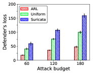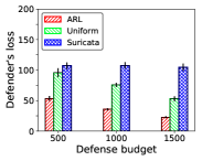
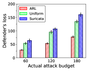
Figure 4 presents our evaluation of the robustness of alert prioritization approaches when the defender knows the adversary’s capabilities, and the results suggest that our approach significantly outperforms the other baselines. Specifically, the proposed approach is $50\%$ better than the Uniform policy, which in turn is significantly better than using Suricata priorities. There are a few reasons why deterministic priority-based approaches perform so poorly. First, determinism allows attackers to easily circumvent the policy by focusing on attacks that trigger alerts which are rarely inspected. Moreover, such naive deterministic policies also fail to exploit the empirical relationships between attacks and alerts they tend to trigger: for example, if an attack triggers multiple alerts, but one of these alert types happens to have very few alerts in current logs, static priority-based policies will not leverage this structure. In contrast, by learning a policy of alert inspection which maps arbitrary alert observations to a decision about which to inspect, we can make decisions at a significantly finer granularity.

Figure 5: Intrusion detection: loss of the defender when it is uncertain of the attack budget. Left: def. budget=500. Right: def. budget=1500. The defender’s estimate of the attack budget is 120 in all cases. Thus, if the actual attack budget is 60, then the defender overestimates the adversary’s budget; if the actual attack budget is 180, then it is underestimated by the defender.

Figure 6: Intrusion detection: loss of the defender when it has different estimates of the attack budget.

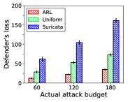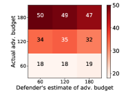
Evaluating the alert prioritization methods when the defender is uncertain about the attack budget (Figures 5 and 6), we can observe that the proposed ARL approach still achieves the lowest defender loss both when the attack budget is underestimated and when overestimated, and it is still far better than the baselines. In addition, Figure 6 shows that when the attack budget is underestimated or overestimated, there is only a $5\%$ performance degradation compared to when the defender has full knowledge of the adversary. This demonstrates that our approach remains robust to a strategic adversary even when the defender does not precisely know the adversary’s capabilities. Moreover, in this domain we can see that neither over- nor underestimating adversary’s budget is particularly harmful, although overestimation appears to be slightly better.

Figure 7: Intrusion detection: loss of the defender when it is certain of the attack budget but is uncertain of the attack policy. The attack budget is fixed as 120. Left: def. budget=500. Right: def. budget=1500.

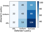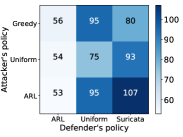
Our final consideration is the impact of uncertainty about the adversary’s rationality (Figure 7). Specifically, we now study how our approach performs, compared to the baselines, if the adversary is in some way myopic, either using a simple uniform strategy (Uniform) or greedily choosing attacks in order of impact (Greedy). We can observe that although we assume a very strong adversary, our ARL approach significantly outperforms the other baselines even when the adversary is using a different attack policy.

V-C Case Study II: Fraud Detection

While IDS settings are a natural fit for our approach, we now demonstrate its generalizability by considering a very different problem in which our goal is to identify fraudulent credit card transactions. Just as with the first case study, we will present the results first when the defender has full knowledge of the adversary’s capabilities, and subsequently study the impact of defender’s uncertainty about these.

V-C1 Fraud dataset

The fraud dataset contains 284,807 credit card transactions, of which 482 are fraudulent. Each transaction is represented by a vector of 30 numerical features, 28 of which are transformed using Principle Component Analysis (PCA). In addition, each feature vector is associated with a binary label indicating the type of transaction (regular or fraudulent). In order to make it meaningful in our context, we cluster the set of fraudulent transactions into $n$ subsets, indicating a type of attack, using a Gaussian Mixture model [5]. In our experiments, we set $n=6$, and modify the dataset with fraudulent labels replaced by cluster assignments. The counts of each type of transaction is shown in Table VI.

TABLE VI: Number of transactions in the modified fraud dataset

Original transaction type	Label	Count
Genuine	0	284,308
Fraudulent	1	11
	2	21
	3	72
	4	250
	5	14
	6	124

V-C2 Learning-based fraud detector

We developed a fraud detector using supervised learning on the fraud dataset. The main challenge is that the dataset is highly imbalanced, as shown in Table VI: the fraudulent transactions only account for $<0.2\%$ of all transactions. To address this challenge, we apply Synthetic Minority Over-sampling Technique (SMOTE) to produce synthetic data for the minority classes to balance the data. Our implementation contains the following steps:

(i) Dataset splitting: We use stratified split to partition the modified fraud dataset into training and test data with equal size, which contain roughly the same proportions of the fraudulent and non-fraudulent data.

(ii) Binary classification: We use SMOTE and linear SVM to learn a binary classifier to predict whether a transaction is fraudulent. The resulting classifier has an AUC $>$99% and a recall $>$90% on the test data, which indicates that more than $90\%$ of the fraudulent transactions can be detected.

(iii) Multi-class classification: We now restrict attention to only the fraudulent transactions to learn a conditional classifier to predict the type of fraud. Specifically, we learn 6 independent classifiers each of which corresponds to one fraud type and returns a binary classification result indicating whether a fraudulent transaction belongs to this type. Similarly to Step (ii), we use SMOTE and linear SVM to learn these classifiers, each of which admits $>94\%$ recall.

Once the fraud detector is implemented, we evaluate the detector using the test dataset. We first predict the test data by using the binary classifier obtained in Step (ii) above. If any transaction in the test data is classified as fraudulent, then it is further inspected by the 6 classifiers we construct for multi-class classification. If a fraudulent transaction is predicted as any type of fraud, then a corresponding alert is triggered. Otherwise, an alert corresponding to the fraud type which is predicted with the highest classification score is triggered.

V-C3 Experimental Setup

To evaluate the robustness of the proposed approach for alert prioritization in fraud detection, we first computed the distributions of the true and false alerts identified by the fraud detector that we implemented. By doing so, we obtained the probability that any attack $a\in A$ triggers an alert $t\in T$, as well as the number of false alarms associated with each type of alert, each of which has a value of 1 as the investigation cost. We filtered out alert types that were triggered only by fraudulent transactions (as we had done before), leaving 3 out of 6 alert types. We also filtered out the attack actions which are associated with the alert types omitted above, as these attacks can always be detected by investigating the corresponding alerts. The resulting distribution of the alerts triggered by frauds is given in Table VII.

TABLE VII: Probability that an attack action triggers each type of alert

Attack action	Alert type
	1	2	3
1	0.9	0.61	0
2	0.09	0.87	0.12
3	0	0.41	0.85

We used $[1,3,2]$ as the adversary’s cost of the mounting each type of attack action. We employed the mean amount of each type of fraudulent transaction as the loss of the defender if any such type of attack action is not detected, measured by the unit of 10 Euros. The corresponding defender’s loss for each undetected attack was $[9.4,12.1,16.0]$. In addition, we used 30 minutes as the fixed length of each time period in our experiments. Based on our classification results, the average number of false alerts that occur of each type in a time period was $[10,47,39]$. Similar to our IDS case study, we simulated the distribution of false alerts by using Poisson processes with the above mean values.

V-C4 Baselines

The performance of the proposed approach is investigated by comparing with three alternative policies for alert prioritization: Uniform, a policy which uniformly allocates the defender’s budget over each alert type; GAIN [19], a game theoretic approach which prioritizes alert types, and always inspects all alerts of a selected type; and RIO [43], another game theoretic approach which prioritizes alerts, and computes an approximately optimal number of alerts of each type to inspect.

V-C5 Results

Figure 8: Fraud detection: loss of the defender when it knows the attack budget. Left: Defender’s loss by its budget, with attack budget adv_budget being fixed as 2. Right: Defender’s loss by attack budget, with defense budget def_budget being fixed as 20.

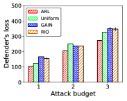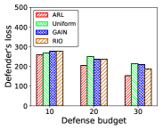
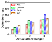
Figure 8 shows the results when the defender has full knowledge of the adversary’s capabilities. We can observe that the proposed approach (ARL) outperforms other baselines in all settings, typically by at least $25\%$. The main reason for the advantage is similar to that in the IDS setting: the ability to have a policy that is carefully optimized and conditional on state significantly increases its efficiency. Interestingly, the alternative game theoretic alert prioritization approaches, GAIN and RIO, are in some cases worse than the uniformly random policy. The key reason is that they can be myopic in that they independently optimize for a single time period, whereas attacks can be adaptive. The proposed approach, in contrast, explicitly considers such adaptivity.

Figure 9: Fraud detection: loss of the defender when it is uncertain of the attack budget. Left: def. budget=10. Right: def. budget=30. The defender’s estimate of the attack budget is 2. If the actual attack budget is 1, then the defender overestimates the adversary’s budget; if the actual attack budget is 3, then it is underestimated.

Figure 10: Fraud detection: loss of the defender when it has different estimates of the attack budget.

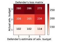
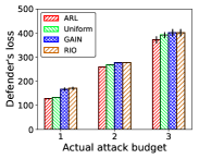
Figures 9 and 10 investigate performance of our approach when the attack budget is uncertain. It can be seen in Figure 9 that ARL remains the best approach to use, despite this uncertainty. Interestingly, GAIN can, in contrast, be rather fragile to such uncertainty. Considering Figure 10, both under- and overestimation of the attack budget incurs a limited performance impact ($<10\%$). More interesting, however, is the observation that it is actually better to slightly underestimate the adversary’s budget: in the worst case, this hurts performance less than $3\%$. Effectively, the approach remains quite robust even against stronger attacks, whereas overestimating the budget does not take sufficient advantage of weaker adversaries.

Figure 11: Fraud detection: loss of the defender when it is certain of the attack budget but is uncertain of the attack policy. The attack budget is fixed as 2. Left: def. budget=10. Right: def. budget=30.

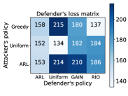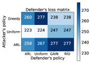
Finally, we study the robustness of ARL compared to other baselines when the attacker is using different policies (Uniform or Greedy) instead of the RL-based policy that is assumed by our approach (Figure 11). Here, the results are slightly more ambiguous than we observed in the IDS domain: when the adversary is using the Greedy policy, RIO does outperform ARL by $8\%$ when the defender’s budget is small, and by $13\%$ when the defender’s budget is large. However, in these cases, the adversary can gain a great deal by more carefully designing its policy. Thus, when the defender’s budget is large, a rational adversary can cause RIO to degrade by nearly $18\%$, where ARL is quite robust to such adversaries.

VI Related Work

VI-A Deep Reinforcement Learning

Reinforcement learning has received significant attention in recent years, which is in large part due to the emergence of deep reinforcement learning. Deep reinforcement learning combines classic reinforcement learning approaches, such as Q-learning [42], with deep neural networks. Classic Q-learning is a model-free reinforcement learning approach, which is guaranteed to find an optimal policy for any finite Markov decision process [41]. However, to do so, it needs to learn and store an exact representation of the action-value function, which is infeasible for a problem with large action or state spaces. Notable early successes combining reinforcement learning with neural networks include TD-Gammon, a backgammon program that achieved a level of play that was comparable to top human players in 1992 [35]. More recently, Mnih et al. introduced the model-free Deep Q-Learning algorithm (DQN), which achieved human-level performance in playing a number of Atari videogames, using purely visual input from the games [28, 29]. However, the actions spaces in all of these games were small and discrete. Lillicrap et al. adapted the idea of Deep Q-Learning to continuous action spaces by introducing an algorithm, called Deep Deterministic Policy Gradient (DDPG) [20]. DDPG is a model-free actor-critic algorithm, whose robustness is demonstrated on a variety of continuous control tasks. Hessel et al. evaluated six improvements to the DQN algorithm (DDQN [37], Prioritized DDQN [31], Dueling DDQN [40], A3C [27], Distributional DQN [4], and Noisy DQN [9]), which had been proposed by the deep reinforcement learning community since the publication of DQN, across 57 Atari games [12]. Further, they integrated these improvements into a single agent, called Rainbow, and demonstrated its state-of-the-art performance on common benchmarks.

VI-B Multi-agent Reinforcement Learning

Single-agent reinforcement learning approaches can train only one agent at a time, which means that in a multi-agent setting, they must treat other agents as part of the environment. As a result, they often provide policies that are not robust—especially in a non-cooperative setting such as ours—since they cannot consider the possibility that other agents respond by learning and updating their own policies. Multi-agent reinforcement learning approaches attempt to provide more robust policies by training multiple adaptive agents together.

Littman proposed a framework for multi-agent reinforcement learning that models the competition between two agents as a zero-sum Markov game [21]. To solve this game, the author introduced a Q-learning-like algorithm, called minimax-Q, which is guaranteed to converge to optimal policies for both players. However, the minimax-Q algorithm assumes that the game is zero-sum (i.e., the player’s rewards are exact opposites of each other) and every step of the training involves exhaustive searches over the action spaces, which limits the applicability of the algorithm. A number of follow up efforts have proposed more general solutions. For example, Hu and Wellman extended Littman’s framework to general-sum stochastic games [15]. They propose an algorithm that is based on each agent learning two action-value functions (one for itself and one for its opponent), which is guaranteed to converge to a Nash equilibrium under certain conditions. To relax some of these conditions, Littman introduced Friend-or-Foe Q-learning, in which each agent is told to treat each other agent either as a “friend” or as a “foe” [22]. Later, Hu and Wellman proposed the NashQ algorithm, which generalizes single-agent Q-learning to stochastic games with many agents by using an equilibrium operator instead of expected utility maximization [14].

While the above approaches have the advantage of providing certain convergence guarantees, they assume that action-value functions are represented exactly, which is infeasible for scenarios with large action or state spaces. Deep multi-agent reinforcement-learning provides a more scalable approach by representing action-value functions using deep neural networks. For example, Lowe et al. proposed an adaptation of actor-critic reinforcement-learning methods to multi-agent settings [23]. In the proposed approach, each agent learns a collection of different sub-policies, and for each episode, each agent randomly selects sub-policy from this collection. However, in contrast to our approach, the size of the collection is fixed (which may waste training effort at the beginning and might not converge in the end) and the agents choose their sub-policies at random instead of strategically. Lanctot et al. introduced an algorithm, called policy-space response oracles, which is closer to our double-oracle based computational approach [18]. Their proposed algorithm maintains a set of policies for each agent, but it does not incorporate actor-critic methods, and it was evaluated in settings with relatively small discrete action spaces.

VI-C Alert Management and Prioritization

A multitude of research efforts have studied the problem of reducing the number of alerts without significantly reducing the probability of attack detection [16]. One of the most common approaches is alert correlation and clustering, which attempt to group related alerts together, thereby reducing the set of messages that are presented [30]. In distributed systems, collaborative intrusion detection systems may be deployed, which include several monitoring components and correlate alerts among the monitors to create a holistic view [38]. Since the number of alerts may be too high even after correlation, research efforts have also investigated the prioritization of alerts. For example, Alsubhi et al. introduced a fuzzy-logic based alert management system, called FuzMet, which uses several metrics and fuzzy logic to score and prioritize alerts [2]. However, these approaches do not consider the possibility of an attacker adapting to the prioritization.

VI-D Game Theory for Alert Prioritization and Security Audits

Prior work has successfully applied game theory to a variety of security problems, ranging from physical security [3] to network security and privacy [24].

Our approach is most closely related to alert-prioritization games. Laszka et al. introduced the first game-theoretic model for alert prioritization, which they solved with the help of a greedy heuristic [19]. The performance of this approach, which we denoted GAIN in our experiments, is limited by its restrictive assumptions about the defender’s decision making. In particular, GAIN assumes that the defender’s policy is a strict prioritization that investigates all higher-priority alerts before investigating any lower-priority ones, and the prioritization is chosen before observing the actual number of alerts. Moreover, the model considers only a single time slot, which further limits its usefulness. Yan et al. improved upon GAIN by allowing the defender to specify a maximum budget that may be spent on each alert types, thereby relaxing the strict prioritization of GAIN [43]. However, this improved approach, which we denoted RIO in our experiments, still assumes that the prioritization is chosen before observing any alerts and considers only a single time slot. As our numerical results demonstrate, these restrictions can lead to significantly higher losses for the defender. Schlenker et al. introduced a similar model, called Cyber-alert Allocation Game, which further simplifies the problem by assuming that the number of false alerts is fixed and known by both parties in advance [32].

Our approach also resembles audit games, which study the problem of allocating a limited amount of audit resources to a fixed number of audit targets [6, 7]. However, despite the resemblance, audit games are ill-suited for prioritizing alerts since these games assume that the attacker knows the exact set of targets, which would correspond to individual alerts, before launching its attack. Due to the unpredictability of false alerts, this assumption does not hold for alert prioritization.

VII Discussion and Conclusion

Since even after applying techniques for reducing the alert burden (e.g., alert correlation) there often remain vastly more alerts than time to investigate them, the success of detection often hinges on how defenders prioritize certain alerts over others. In practice, prioritization is typically based on non-strategic heuristics (e.g., Suricata’s built-in priority values), which may easily be exploited by a strategic attacker who can adapt to the prioritization. Strategic prioritization approaches attempt to prevent this by using game-theory to capture adaptive attackers; however, existing strategic approaches severely restrict the defender’s policy (e.g., strict prioritization) for the sake of computational tractability.

In contrast, we introduced a general model of alert prioritization that does not impose any restrictions on the defender’s policy, and we proposed a novel double oracle and reinforcement learning based approach for finding approximately optimal prioritization policies efficiently. Our experimental results—based on case studies of IDS and fraud detection—demonstrate that these policies significantly outperform non-strategic prioritization and prior game-theoretic approaches. Further, to demonstrate the strength of our attacker model, we also showed that the attacker policies found by our approach outperform multiple baseline policies.

For practitioners, the key task in applying our approach is estimating the parameter values of our model. In our case studies, we showed how to estimate parameters in two domains (e.g., for IDS, using CVSS score to estimate attack impact and CVSS complexity for attack cost). The most difficult parameter to estimate is the attacker’s budget; however, our experimental results show that our approach is robust to uncertainty in the attacker’s budget and outperforms other approaches even when the budget is misestimated. We leave studying the sensitivity to other parameters to future work.

-A Best Response Oracle Algorithm

The proposed algorithm to compute the best response oracle is outlined in Algorithm 1.

Algorithm 1 DDPG-MIX Algorithm: Compute the pure-strategy best response of player $v$ when its opponent takes mixed-strategy $\bm{\sigma}_{-v}$.

0:    The set of opponent’s pure strategies, $\bm{\Pi}_{-v}$; Mixed strategy of the opponent, $\bm{\sigma}_{-v}$;

0:    The value network of player $v$, $Q_{v}(\bm{O}_{v},\bm{\alpha}_{v}|\bm{\theta}_{v}^{Q})$; The policy network of player $v$, $\bm{\pi}_{v}(\bm{O}_{v}|\bm{\theta}_{v}^{\pi})$;

1:  Randomly initialize $Q_{v}(\bm{O}_{v},\bm{\alpha}_{v}|\bm{\theta}_{v}^{Q})$ and $\bm{\pi}_{v}(\bm{O}_{v}|\bm{\theta}_{v}^{\pi})$;

2:  Initialize replay memory $\mathcal{D}$;

3:  for $episode=0,M-1$ do

4:     Initialize the system state $\langle\bm{N}^{(0)},\bm{M}^{(0)},\bm{S}^{(0)}\rangle=\langle\bm{0},\bm{0},\bm{0}\rangle$;

5:     Sample the opponent’s policy $\bm{\pi}_{-v}$ by using $\bm{\sigma}_{-v}$ over $\bm{\Pi}_{-v}$;

6:     for $k=0,K-1$ do

7:        With probability $\epsilon$ select a random action $\bm{\alpha}_{v}^{(k)}$; Otherwise, select $\bm{\alpha}_{v}^{(k)}=\bm{\pi}_{v}(\bm{O}_{v}^{(k)}|\bm{\theta}_{v}^{\mu})$;

8:        Execute $\bm{\alpha}_{v}^{(k)}$ and $\bm{\alpha}_{-v}^{(k)}=\bm{\pi}_{-v}(\bm{O}_{-v}^{(k)})$, observe reward $r_{v}^{(k)}$ and transit the system state to $\bm{S}^{k+1}$;

9:        Store transition $(\bm{O}_{v}^{(k)},\bm{\alpha}_{v}^{(k)},r_{v}^{(k)},\bm{O}_{v}^{(k+1)})$ in $\mathcal{D}$;

10:        Sample a random minibatch of $N$ transitions $(\bm{O}_{v}^{(i)},\bm{\alpha}_{v}^{(i)},r_{v}^{(i)},\bm{O}_{v}^{(i+1)})$ from $\mathcal{D}$;

11:        Set $y_{v}^{(i)}=r_{v}^{(i)}+\tau Q_{v}(\bm{O}_{v}^{(i+1)},\bm{\pi}(\bm{O}_{v}^{(i+1)}|\bm{\theta}^{\pi}_{v})|\bm{\theta}^{Q}_{v})$;

12:        Update the value network by minimizing the loss

$$\mathcal{L}(\bm{\theta}^{Q}_{v})=\frac{1}{N}\sum_{i}(y_{v}^{(i)}-Q_{v}(\bm{O}_{v}^{i},\bm{\alpha}_{v}^{(i)}|\bm{\theta}^{Q}_{v}))^{2};$$

13:        Update the policy network by using the sampled policy gradient:

$$\nabla_{\bm{\theta}_{v}^{\pi}}\mathcal{J}\approx\frac{1}{N}\sum_{i}J_{a}\cdot J_{\theta}$$ (12)

where

$$\begin{cases}J_{a}=\nabla_{\bm{\alpha}_{v}}Q_{v}(\bm{O}_{v},\bm{\alpha}_{v}|\bm{\theta}^{Q}_{v})|_{\bm{O}_{v}=\bm{O}_{v}^{(i)},\bm{\alpha}_{v}=\bm{\pi}_{v}(\bm{O}_{v}^{(i)})}\\ J_{\theta}=\nabla_{\bm{\theta}_{v}^{\pi}}\bm{\pi}(\bm{O}_{v}|\bm{\theta}_{v}^{\pi})|_{\bm{O}_{v}^{(i)}}\end{cases}$$ (13)

14:     end for

15:  end for

16:  return  Player $v$’s policy network, $\bm{\pi}_{v}(\bm{O}_{v}|\bm{\theta}_{v}^{\pi})$.

-B Computational Cost

Figure 12: Computational cost. Left: Number of double oracle iterations in intrusion detection with adv. budget=120. Right: Number of double oracle iterations in fraud detection with adv. budget=2.

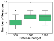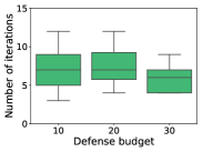Figure 12 presents our evaluation of the computational cost of the proposed alert prioritization approach. The results show that the double oracle algorithm can converge very fast in practice, with fewer than 15 iterations in most cases; indeed, in the vast majority of instances we need fewer than 10 iterations.

Another interesting observation is non-monotonicity of convergence time (in terms of iterations) as we increase the defense budget. In the IDS setting, for example, increasing the defense budget increases the number of iterations when we go from a budget of 500 to 1000, but the computational cost remains stable as we further increase the budget to 1500. In contrast, in the fraud detection case study, increasing the budget from 10 to 20 has little impact on the number of iterations, but further increasing it to 30 actually reduces the number of iterations necessary for convergence. To understand this phenomenon, note that increasing the defender’s budget has two opposing effects: on the one hand, the search space for the defender increases significantly, but on the other hand, it may become much easier to compute a near-optimal defense with a larger budget (for example, with a large enough budget, we can almost always inspect all alerts).

References

- [1] M. Abadi, P. Barham, J. Chen, Z. Chen, A. Davis, J. Dean, M. Devin, S. Ghemawat, G. Irving, M. Isard, M. Kudlur, J. Levenberg, R. Monga, S. Moore, D. G. Murray, B. Steiner, P. Tucker, V. Vasudevan, P. Warden, M. Wicke, Y. Yu, and X. Zheng, “TensorFlow: A system for large-scale machine learning,” in Proceedings of the 12th USENIX Symposium on Operating Systems Design and Implementation, 2016, pp. 265–283.
- [2] K. Alsubhi, I. Aib, and R. Boutaba, “FuzMet: A fuzzy-logic based alert prioritization engine for intrusion detection systems,” International Journal of Network Management, vol. 22, no. 4, pp. 263–284, 2012.
- [3] B. An, F. Ordóñez, M. Tambe, E. Shieh, R. Yang, C. Baldwin, J. DiRenzo III, K. Moretti, B. Maule, and G. Meyer, “A deployed quantal response-based patrol planning system for the US Coast Guard,” Interfaces, vol. 43, no. 5, pp. 400–420, 2013.
- [4] M. G. Bellemare, W. Dabney, and R. Munos, “A distributional perspective on reinforcement learning,” in Proceedings of the 34th International Conference on Machine Learning (ICML) – Volume 70. JMLR, 2017, pp. 449–458.
- [5] C. M. Bishop, Pattern Recognition and Machine Learning, ser. Information Science and Statistics. Springer, 2011.
- [6] J. Blocki, N. Christin, A. Datta, A. D. Procaccia, and A. Sinha, “Audit games,” in Proceedings of the 23rd International Joint Conference on Artificial Intelligence (IJCAI), ser. IJCAI ’13. AAAI Press, 2013, pp. 41–47. [Online]. Available: http://dl.acm.org/citation.cfm?id=2540128.2540137
- [7] ——, “Audit games with multiple defender resources,” in Proceedings of the 29th AAAI Conference on Artificial Intelligence, 2015.
- [8] A. L. Buczak and E. Guven, “A survey of data mining and machine learning methods for cyber security intrusion detection,” IEEE Communications Surveys & Tutorials, vol. 18, no. 2, pp. 1153–1176, 2016.
- [9] M. Fortunato, M. G. Azar, B. Piot, J. Menick, I. Osband, A. Graves, V. Mnih, R. Munos, D. Hassabis, O. Pietquin et al., “Noisy networks for exploration,” arXiv preprint arXiv:1706.10295, 2017.
- [10] X. Glorot and Y. Bengio, “Understanding the difficulty of training deep feedforward neural networks,” in Proceedings of the 13th international conference on artificial intelligence and statistics (AISTAT), 2010, pp. 249–256.
- [11] K. He, X. Zhang, S. Ren, and J. Sun, “Delving deep into rectifiers: Surpassing human-level performance on imagenet classification,” in Proceedings of the 2015 IEEE International Conference on Computer Vision (ICCV), 2015, pp. 1026–1034.
- [12] M. Hessel, J. Modayil, H. Van Hasselt, T. Schaul, G. Ostrovski, W. Dabney, D. Horgan, B. Piot, M. Azar, and D. Silver, “Rainbow: Combining improvements in deep reinforcement learning,” in Proceedings of the 32nd AAAI Conference on Artificial Intelligence, ser. AAAI, 2018.
- [13] G. Ho, A. Sharma, M. Javed, V. Paxson, and D. Wagner, “Detecting credential spearphishing in enterprise settings,” in Proceedings of the 26th USENIX Security Symposium (USENIX Security), 2017, pp. 469–485.
- [14] J. Hu and M. P. Wellman, “Nash Q-learning for general-sum stochastic games,” Journal of Machine Learning Research, vol. 4, no. Nov, pp. 1039–1069, 2003.
- [15] J. Hu, M. P. Wellman et al., “Multiagent reinforcement learning: theoretical framework and an algorithm,” in Proceedings of the 15th International Conference on Machine Learning (ICML), vol. 98, 1998, pp. 242–250.
- [16] N. Hubballi and V. Suryanarayanan, “False alarm minimization techniques in signature-based intrusion detection systems: A survey,” Computer Communications, vol. 49, pp. 1–17, 2014.
- [17] D. Korzhyk, Z. Yin, C. Kiekintveld, V. Conitzer, and M. Tambe, “Stackelberg vs. Nash in security games: An extended investigation of interchangeability, equivalence, and uniqueness,” Journal of Artificial Intelligence Research, vol. 41, pp. 297–327, 2011.
- [18] M. Lanctot, V. Zambaldi, A. Gruslys, A. Lazaridou, K. Tuyls, J. Pérolat, D. Silver, and T. Graepel, “A unified game-theoretic approach to multiagent reinforcement learning,” in Proceedings of the 31st International Conference on Neural Information Processing Systems (NIPS), 2017, pp. 4193–4206.
- [19] A. Laszka, Y. Vorobeychik, D. Fabbri, C. Yan, and B. Malin, “A game-theoretic approach for alert prioritization,” in AAAI Workshop on Artificial Intelligence for Cyber Security (AICS), Febrary 2017.
- [20] T. P. Lillicrap, J. J. Hunt, A. Pritzel, N. Heess, T. Erez, Y. Tassa, D. Silver, and D. Wierstra, “Continuous control with deep reinforcement learning,” arXiv preprint arXiv:1509.02971, 2015.
- [21] M. L. Littman, “Markov games as a framework for multi-agent reinforcement learning,” in Proceedings of the 11th International Conference on International Conference on Machine Learning (ICML). Elsevier, 1994, pp. 157–163.
- [22] ——, “Friend-or-foe Q-learning in general-sum games,” in Proceedings of the 18th International Conference on Machine Learning (ICML), vol. 1, 2001, pp. 322–328.
- [23] R. Lowe, Y. Wu, A. Tamar, J. Harb, P. Abbeel, and I. Mordatch, “Multi-agent actor-critic for mixed cooperative-competitive environments,” in Proceedings of the 31st International Conference on Neural Information Processing Systems (NIPS), 2017, pp. 6382–6393.
- [24] M. H. Manshaei, Q. Zhu, T. Alpcan, T. Bacşar, and J.-P. Hubaux, “Game theory meets network security and privacy,” ACM Computing Surveys (CSUR), vol. 45, no. 3, p. 25, 2013.
- [25] H. B. McMahan, G. J. Gordon, and A. Blum, “Planning in the presence of cost functions controlled by an adversary,” in Proceedings of the 20th International Conference on Machine Learning (ICML), 2003, p. 536–543.
- [26] A. Milenkoski, M. Vieira, S. Kounev, A. Avritzer, and B. D. Payne, “Evaluating computer intrusion detection systems: A survey of common practices,” ACM Computing Surveys (CSUR), vol. 48, no. 1, p. 12, 2015.
- [27] V. Mnih, A. P. Badia, M. Mirza, A. Graves, T. Lillicrap, T. Harley, D. Silver, and K. Kavukcuoglu, “Asynchronous methods for deep reinforcement learning,” in Proceedings of the 33rd International Conference on International Conference on Machine Learning (ICML) – Volume 48, 2016, pp. 1928–1937.
- [28] V. Mnih, K. Kavukcuoglu, D. Silver, A. Graves, I. Antonoglou, D. Wierstra, and M. Riedmiller, “Playing Atari with deep reinforcement learning,” arXiv preprint arXiv:1312.5602, 2013.
- [29] V. Mnih, K. Kavukcuoglu, D. Silver, A. A. Rusu, J. Veness, M. G. Bellemare, A. Graves, M. Riedmiller, A. K. Fidjeland, G. Ostrovski et al., “Human-level control through deep reinforcement learning,” Nature, vol. 518, no. 7540, p. 529, 2015.
- [30] S. Salah, G. Maciá-Fernández, and J. E. DíAz-Verdejo, “A model-based survey of alert correlation techniques,” Computer Networks, vol. 57, no. 5, pp. 1289–1317, 2013.
- [31] T. Schaul, J. Quan, I. Antonoglou, and D. Silver, “Prioritized experience replay,” arXiv preprint arXiv:1511.05952, 2015.
- [32] A. Schlenker, H. Xu, M. Guirguis, C. Kiekintveld, A. Sinha, M. Tambe, S. Sonya, D. Balderas, and N. Dunstatter, “Don’t bury your head in warnings: A game-theoretic approach for intelligent allocation of cyber-security alerts,” in Proceedings of the 26th International Joint Conference on Artificial Intelligence (IJCAI), 2017, pp. 381–387. [Online]. Available: https://doi.org/10.24963/ijcai.2017/54
- [33] I. Sharafaldin, A. Habibi Lashkari, and A. A. Ghorbani, “Toward generating a new intrusion detection dataset and intrusion traffic characterization,” in Proceedings of the 4th International Conference on Information Systems Security and Privacy (ICISSP) – Volume 1, INSTICC. SciTePress, 2018, pp. 108–116.
- [34] R. Sommer and V. Paxson, “Outside the closed world: On using machine learning for network intrusion detection,” in 2010 IEEE symposium on security and privacy. IEEE, 2010, pp. 305–316.
- [35] G. Tesauro, “TD-Gammon, a self-teaching backgammon program, achieves master-level play,” Neural Computation, vol. 6, no. 2, pp. 215–219, 1994.
- [36] J. Tsai, T. H. Nguyen, and M. Tambe, “Security games for controlling contagion,” in Proceedings of the 26th AAAI Conference on Artificial Intelligence, ser. AAAI’12. AAAI Press, 2012, pp. 1464–1470. [Online]. Available: http://dl.acm.org/citation.cfm?id=2900929.2900936
- [37] H. Van Hasselt, A. Guez, and D. Silver, “Deep reinforcement learning with double Q-learning,” in Proceedings of the 30th AAAI Conference on Artificial Intelligence, 2016.
- [38] E. Vasilomanolakis, S. Karuppayah, M. Mühlhäuser, and M. Fischer, “Taxonomy and survey of collaborative intrusion detection,” ACM Computing Surveys (CSUR), vol. 47, no. 4, p. 55, 2015.
- [39] Y. Vorobeychik and M. Kantarcioglu, Adversarial Machine Learning. Morgan and Claypool, 2018.
- [40] Z. Wang, T. Schaul, M. Hessel, H. Hasselt, M. Lanctot, and N. Freitas, “Dueling network architectures for deep reinforcement learning,” in Proceedings of the 33rd International Conference on International Conference on Machine Learning (ICML), 2016, pp. 1995–2003.
- [41] C. J. Watkins and P. Dayan, “Q-learning,” Machine learning, vol. 8, no. 3-4, pp. 279–292, 1992.
- [42] C. J. C. H. Watkins, “Learning from delayed rewards,” Ph.D. dissertation, King’s College, Cambridge, 1989.
- [43] C. Yan, B. Li, Y. Vorobeychik, A. Laszka, D. Fabbri, and B. Malin, “Get your workload in order: Game theoretic prioritization of database auditing,” in Proceedings of the 34th IEEE International Conference on Data Engineering (ICDE), April 2018, pp. 1304–1307.