The polarized signal from broad emmission lines in AGN

Abstract

Using the STOKES Monte Carlo radiative transfer code we revisit the predictions of the spectropolarimetric signal from a disc-like Broad Emission Line Region (BLR) in Type I AGN due to equatorial scattering. We reproduce the findings of previous works, but only for a scatterer which is much more optically and geometrically thick than previously proposed. We also find that when taking into account the polarized emission from all regions of the scatterer, the swing of the Polarizarion Angle (PA) is in the opposite direction to that originally proposed. Furthermore, we find that the presence of outflows in the scattering media can significantly change the observed line profiles, with the PA of the scattering signal being enhanced in the presence of radially outflowing winds. Finally, a characteristically different PA profile, shaped like an ‘M’, is seen when the scatterer is cospatial with the BLR and radially outflowing.

1 Introduction

A characterization of the geometry and dynamics of the Broad Emission Line Region (BLR) in Active Galactic Nuclei (AGN) has long been the subject of intensive research. Some direct observations have now been made by infrared interferometry on a single target (GRAVITY collaboration et al. 2018) and, more generally, there is mounting evidence that the BLR is likely a flattened system in Keplerian orbits around the central black hole, with a possible contribution from a wind component which seems to be more significant in high ionization lines (Mejía-Restrepo et al. 2018, Shen & Ho 2014, Pancoast et al. 2014, Runnoe et al. 2013, Proga & Kurosawa 2010, Eracleous & Halpern 2003, 1994, Kollatschny 2003, Murray & Chiang 1997, Chiang & Murray 1996, Marziani et al. 1996, Collin-Souffrin et al. 1988, Wills & Browne 1986).

Spectropolarimetry can be an extremely useful tool when addressing the geometry and dynamics of the BLR. This technique adds two new observables to those already available from the analysis of direct light: the degree ($p$) and on-sky position angle (PA) of the polarization of the line and continuum emission which gives information about the scattering processes close to the central engine as a function of velocity. Spectropolarimetry can also give an indirect view of the observed system: that seen by the polarizing material if the polarization is due to scattering. This was clearly demonstrated over 35 years ago by the confirmation that type II AGN (i.e., those where we do not have a direct view of the BLR) can show broad components in their Balmer lines when viewed in polarized light (e.g., Antonucci 1993 and references therein). In these sources the PA is usually perpendicular to the axis of symmetry of the central engine, implying that the light is polarized through scattering from electrons or dust particles located above and/or below the central region.

In a seminal work by Wood, Brown & Fox (1993), changes in polarized flux and PA were studied for the case of Thompson scattering from a disc around line-emitting Be stars. Astonishingly, their analytic work presents, to first approximation, many results with similar line profiles to those presented here, although not always due to the same geometric and dynamical considerations.

Later, Smith et al. (2002, 2004, 2005) published a series of papers looking at spectropolarimetric data for type I AGN (i.e., those where we have a direct view of the BLR) and showed that the continuum polarization is usually parallel to the axis of symmetry of the systems, suggesting that the scattering material must be located in the equatorial plane of the central source (as first pointed out by Brown & McLean 1977 and Shakhovskoi 1965).

The data also showed that the PA ‘swings’ across the Balmer lines which can be explained if the BLR has a disk-like geometry and the scattering region is close enough to the BLR to spatially ‘resolve’ it (this is, that the red and blue Doppler-shifted wings of the emission line are scattered at characteristically different PAs, as viewed by the scatterer).

This understanding of how the inner AGN geometry shapes the polarization across the broad emission lines opens up new possibilities to constrain fundamental parameters of the system. A recent study in this sense was published by Savič et al. (2018), exploring to what extent the BLR polarization can detect Keplerian motion around supermassive black holes and constrain their mass.

The Smith et al. modelling, however, was based on semi-analytical polarization code which considered only one scattering event per line photon. Fast forward 15 years and computers are powerful enough to determine the full Monte Carlo radiative transfer of the continuum and line emission for the different physical, dynamical and geometric conditions of the emitting and scattering regions. In this paper we want to revisit the Smith et al. results and expand their modelling using a physically motivated parameter space of the BLR region and the scattering media around it. In particular, one of the most interesting outcomes, not explored by Smith et al., is found for a coincident BLR/scatterer in the presence of an equatorial wind. Since nuclear winds are thought to be a key component in many AGN, observationally and theoretically, these results open the possibility to study such winds using spectropolarimetry. In fact, we will use such results in an upcoming publication to put real constraints on spectropolarimetric observations of type I AGN and in this way extend our knowledge of the physics of the BLR.

This paper is organized as follows: Section 2 presents the STOKES Monte Carlo code; Section 3 presents our rendition of the Smith et al. (2005) modelling; Sections 4, 5 and 6 present variations and extensions to this paradigm; finally, Section 7 presents our discussion and conclusions.

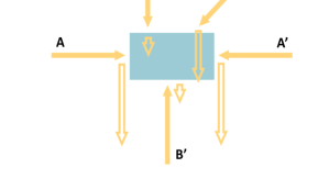
Figure 1: Top: Schematic representation of an anti-clockwise rotating BLR and the inner wall of the scattering region following S05. Only the BLR undergoes Keplerian rotation (green circular arrow), while the scatterer is at rest. The PA is measured West from North (i.e., clockwise) and the observer is located at a very large distance in the southern direction. The near, far and orthogonal locations in the scatterer, as seen by the observer, are shown. At each point of the scatterer inner wall, scattering elements see the velocity resolved BLR line emission with a difference of $\Delta$PA $=\pm 20^{o}$ (red and blue lines, with the black circle also showing the PA of light coming from the region straight ahead, where the continuum source – the accretion disc – is located). S05 predicted that for inclined lines of sight, polarization from the orthogonal regions dominates the polarized signal (regions 1 & 2), as the near and far sides are seen progressively more ‘in transmission’, yielding a net PA $=\pm 20^{o}$ for large inclinations (see bottom figure), as represented in the spectrum presented on the right. Our STOKES realizations show that this is not the case. Bottom: Representation of the polarization degree due to scattering events arriving at a scattering element (blue box) from different directions (A, B and C). The observer is coplanar with the scattering element and situated at the bottom of the figure, while the size of the (empty) arrows after the scattering event shows the level of polarization of the signal. For photons arriving from the sides of the scattering element (A), the polarization degree as measured by the observer will be maximum. For photons arriving from the top and bottom (B), the polarization degree will be minimum – we call this configuration ‘in transmission’. For intermediate directions of the arriving photons (C), intermediate levels of polarization will be seen. Configuration A can explain the level of polarization expected from the orthogonal regions of the scatterer, while configuration B explains the level of polarization expected from the near and far sides.

2 The STOKES Monte Carlo code

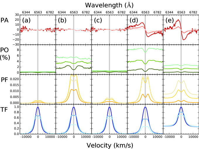
Figure 2: STOKES modelling following the Smith et al. (2005) paradigm for a static equatorial outer scatterer with an electronic density of $1\times 10^{6}$ cm^-3 and a height of 0.001 pc (a), and an electronic density of $3\times 10^{7}$ cm^-3 and a height of 0.01 pc (b). Panels (c) and (d) show the results for the same set of electronic densities but for a scatterer height of 0.03 pc. Panel (e) shows modelling for the same BLR and scatterer parameters as (d) but including the contribution from the continuum unpolarized emission of a central source, with the line flux corresponding to 40% of total flux in the 5800–7200Å range at the innermost radius. In each Panel, from top to bottom, we show the position angle (PA), percentage polarization (PO), polarized flux (PF) and total normalized flux (TF). The three models shown correspond to viewing angles of 24 (dark shades), 41 (medium shades) and 54 (light shades) degrees as measured from the axis of symmetry of the system. Smaller angles yield lower levels of polarization and larger PA changes. The thick grey continuous line corresponds to 0 km/s (6563Å). Notice that subsequent figures do not have the same dynamical ranges in the y-axis.

We use version 1.2 of the Monte Carlo radiative transfer code STOKES presented in Goosmann & Gaskell (2007) and upgraded by Marin et al. (2012). This modelling suite coherently treats three-dimensional radiative transfer and multiple reprocessing between emitting and scattering regions and includes polarization. The system is surrounded by a spherical web of virtual detectors. The detectors record the wavelength, intensity and polarization state of each photon. The latest version of STOKES also generates polarization images with the photons being projected onto the observer’s plane of the sky and then stored in planar coordinates. The net intensity, polarization degree $p$ and polarization position angle PA as a function of wavelength are computed by summing up the STOKES vectors of all detected photons in a given spectral and spatial bin. The spectra can be evaluated at each viewing direction in the polar and azimuthal directions. Note that in this work a PA value equal to zero denotes a polarization state with the E-vector oscillating in a direction parallel to the projected axis of symmetry of the system, while for PA = 90 degrees the E-vector is perpendicular to the projected axis. The PA increases clockwise, i.e., West from North.

In the following Sections we will describe our modelling of the BLR and the scattering media. The dynamical parameterization will be done using cylindrical (v_ρ, v_ϕ, v_z) coordinates. Note also that our BLR is not opaque to photons, i.e., photons can freely cross from one hemisphere to the other. This is in line with the idea of the BLR as a clumpy structure with a small filling factor.

3 The S05 paradigm

The basic set up of parameters in the Smith et al. paradigm can be seen in Table 1 of Smith et al. (2005, hereafter S05). We assume a central black hole of $3.5\times 10^{7}$ M_☉ in mass (compared with a $4.2\times 10^{7}$ M_☉ in S05), surrounded by a Keplerian thin disk BLR (that we assume to have a height of 0.001 pc, as no explicit information is given in S05) with inner and outer radii $3\times 10^{-3}$ and $3\times 10^{-2}$ pc. The line emission generated by this BLR is centered at 6563Å and has an intrinsic width of 50Å or 2286 km/s. A BLR emissivity falling as $\sqrt{R}$ is assumed. The dynamics of the BLR are modelled as nested rings of width 0.001 pc each, for which a Keplerian azimuthal velocity (v_ϕ) is obtained as v${}_{\phi}^{2}=GM/R$, with $G$ the gravitational constant, $M$ the black hole mass and $R$ the radius of the ring.

The scattering region is also thin (again we assume 0.001 pc) and has an annular geometry with inner and outer radii of 0.045 and 0.072 pc, and an initial number density of $10^{6}$ electrons per cubic centimeter, as assumed in S05 (but see below). When a non-stationary scattering medium is assumed, its dynamics — as with the BLR — are modelled as nested rings of width 0.001 pc each with the necessary velocity vectors applied.

STOKES randomly generates isotropically emitted photons in the central continuum source and the BLR, and then follows them as they move freely or are scattered in electron filled regions. Once the photons escape all scattering regions they are registered by the virtual detectors that surround the full $4\pi$ space.

With this set of parameters S05 proposed that for an inclined line of sight (to avoid total cancellation of the polarized signal due to symmetry) the PA of the emission lines ‘swings’ as a function of line velocity with respect to the continuum PA level, with the blue/red wing being above/below (or vice-versa) the continuum level and crossing it at the line center (i.e., at zero velocity), where the velocity vector of the near side of the BLR-disk has no radial component and is located in the same direction as the continuum source (see Figure 1). The wings of the PA profile correspond to those regions with the largest wavelength shifts due to the maximum observable BLR velocity projected along the line of sight, as seen by the scattering elements and located at the innermost of the BLR disk with a PA angle close to zero (depicted as empty red and blue circles in Figure 1). Note that S05 did not include the continuum emission as part of their modelling and only considered the location of the central source at the origin of the coordinate system to determine the continuum PA with respect to that of the emission line.

3.1 General remarks

As already found by S05, Figure 2 shows that the degree of polarization (PO spectrum) increases with inclination angle ($\phi$), as the system appears less and less symmetric to the viewer. In fact, for a pole-on view of the system ($\phi=0$), no polarization is expected as at each wavelength the opposite polarization signal is produced at the opposite side of the disc. However, as soon as the observer has an inclined view of the system, polarization at the near and far sides of the scattering disc should start to diminish as $\cos\phi$ as we see these photons more and more in transmission (which are not polarized); the signal becomes dominated by the polarization from the orthogonal regions of the disc. Our simulations, however, show that while the polarization is indeed dominated by the orthogonal regions, the situation is not symmetric for the near and far sides of the disc due to the thickness of the scatterer, with the far side being more depolarized than the near side because photons have a higher probability of suffering multiple scattering events.

At the same time, the amplitude of the PA swing becomes smaller for more inclined systems, as the change of the sky-projected position angle decreases. This is represented by a PA swing of $\pm 20$ degrees around zero degrees at the orthogonal regions of the disc in Figure 1. Another noticeable result, pointed out by S05, is that the line seen in polarized light (the PF spectrum) is broader than that seen in direct light. This is due to the location of the equatorial scatterer which maximizes the relative projected velocity between the BLR and the scattering region. In other words, the scattering region ‘sees’ the full velocity field and produces a broader, double-horn line, as expected for Keplerian line emitting discs (e.g., Eracleous et al. 2009). This, when combined with the direct emission (the TF spectrum), results in a high percentage polarization (the PO spectrum) of the line wings and a dip at the line center. Finally, as can be seen, the TF spectra have been normalized to the peak flux of the spectrum observed at the smallest inclination angle (24 degrees), which corresponds to the largest solid angle of the BLR as seen by the observer, yielding a larger total flux in the line.

Panel (e) in Figure 2 includes the unpolarized continuum emission from the central source with line emission corresponding to 40% of the total flux in the 5800-7200Å range at the innermost BLR radius and decreasing outwards as the square root of the radius. It can be seen that the main effects of adding the continuum component are the presence of the polarized continuum in the PF spectra and a decrease in the level of polarization across the continuum and line in the PO spectrum due to dilution, making it appear flatter (for a quantitative comparison between models see Table 2). The predicted PO values are very close to those typically observed in type I AGN (e.g., Smith et al. 2002, Schmid et al. 2001, Smith et al. 1997, Goodrich 1989). In addition, the line PA swing becomes more pronounced and the very extended PA wings seen at high velocities are no longer present. The explanation for this requires further consideration.

The changes in the PA behaviour are not due to the geometric configuration of the system, but to the vectorial nature of the polarized signal. The continuum emission is always polarized at a PA equal to the tangential direction of the circles depicted in Figure 1. At each wavelength we need to add the coninuum and line emission, as vectors. But, as already discussed, the PA of the line is constantly rotating as a function of velocity and therefore the result of the vectorial addition will vary with wavelength. The end result is that the PA peaks, which geometrically correspond to the largest opening angles seen by the scattering element (and therefore to intermediate velocities of $\sim\pm 2000$ km/s – see Figure 1), are increased by the addition of the continuum vector, while the high velocity wings beyond $\sim\pm 10000$ km/s are dominated by the zero angle continuum emission.

Since a model including a central emitting source is more realistic than the original S05 scenario, all subsequent models will contain both continuum and line emission. Parameters for the original S05 model, our realization, and subsequent models presented in the following Sections, are given in Table 1.

3.2 The optical depth and covering factor of the scatterer

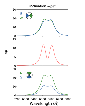
Figure 3: Polarized Flux (PF) as a function of wavelength for the four quadrants of the scattering region for model 2(d). These are the East, West (top panel), North and South (bottom panel) quadrants, as represented by the pie charts. The total spectrum is also presented (middle panel).

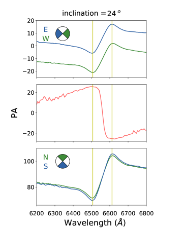
Figure 4: Position angle (PA) as a function of wavelength for the four quadrants of the scattering region for model 2(d). These are the East, West (top panel), North and South (bottom panel) quadrants, as represented by the pie charts. The total spectrum is also presented (middle panel).

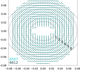
Figure 5: PA spatially resolved maps of model 2(d) for 6507 Å and 6612 Å at a viewing angle of 24 degrees (left) and 41 degrees (right). The markers show the PA orientation and their sizes are arbitrary. The scatterer has been divided into concentric projected-rings. The axes in all plots are expressed in pc.

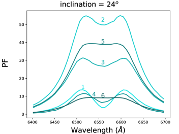
Figure 6: PF spectra obtained from the spatially resolved maps of model 2(d) for a viewing angle of 24 degress. The spectra correspond to the concentric rings represented in Figure 5.

One important element of the S05 paradigm is that the net polarization, and therefore the resulting observed PA, will be dominated by the orthogonal regions of the scatterer, as shown in Figure 1. Those regions found at the near and far side of the scatterer, which are seen progressively more ‘in transmission’ for more inclined views, are mostly canceled out.

We started by computing the polarimetric signal for the original S05 parameter set up. However, we failed to reproduce their results and instead found a very low degree of polarization ($<0.3\%$) with no PA change across the line (see Figure 2, Panel (a)). It soon became clear that a higher density and much larger covering factors were needed to reproduce the line scattering signal. Trial and error showed that electron densities of $\la 10^{7}$ cm^-3 had sufficient optical depth to return higher levels of polarization, but still gave a very low amplitude swing across the emission line (Figure 2, Panel (b)). A dramatic increase in the solid angle of the scatterer as seen by the BLR (from a total height of 0.001, to 0.01 and finally 0.03; see Table 1) is necessary to increase the swing to amplitudes comparable to those observed in Seyfert 1 galaxies (Fig 2, Panel (d)). When comparing with S05 it can be seen that the Monte Carlo code predicts a less sinusoidal-like PA swing, with a slower rise/fall of the high velocity winds.

The large optical depths and covering factors imply an asymmetry between the far and near side of the system. Figure 3 shows the resulting PF spectra after averaging over four different regions of the scatterer: the North, South, East and West quadrants. While back-scattering off the far side (N) of the scattering region gives a high level of polarized flux from photons that can reach the observer, photons that undergo forward-scattering while traveling towards the observer and across the scatterer in the near side (S) yield about half the level of polarized flux. A small difference is also seen in the strength of the blue and red horns between the East and West quadrants. This is a significant departure from the results found by S05.

3.3 The sense of the PA swing

Our simulation show that the swing in the PA spectrum is in the opposite sense to that predicted by S05 and shown in Figure 1, with the blue side of the line seen at positive PA values and the red side at negative PA values. We explain this inversion in the rest of this section.

Figure 4 shows the PA spectra obtained from averaging the STOKES vectors over the N, S, E and W quadrants. All show the PA swing expected from Figure 1. The E and W quadrants average PA, however, is not located at 0 degrees. This is because of the different levels of polarized flux coming from the near and far side of the scatterer, with the emission from the far side being much more dominant, as discussed in the previous section. This biases the resulting average PA of the E and W quadrants towards northern values. This effect goes away in simulations with smaller optical depths.

The spectrum showing the PA obtained when averaging the STOKES parameters over the full scattering region, however, reverts to what was presented in Figure 2. The nearly identical PA signature coming from the N and S quadrants, which are affected by very different optical depths, suggests that optical thickness is not responsible for the reverse in the PA swing. So the sense of the swing of the resulting PA should be due to geometric cancellation between quadrants.

Table 1: Geometric and dynamical parameters of the BLR and scattering regions used for the STOKES modelling.

Model	Broad Line Region					Scatterer
	Rin	Rout	Height	v${}_{\phi}{\dagger}$		Rin	Rout	Height	vρ	v${}_{\phi}{\dagger}$	vz	$\tau_{z}$	$\tau_{r}$	ne
	pc	pc	pc	km/s		pc	pc	pc	km/s	km/s	km/s			cm-3
S05	0.003	0.035	0.001	6736		0.045	0.073	0.001	0	0	0	–	–	1e6
Fig2(a)	0.003	0.035	0.001	6736		0.045	0.073	0.01	0	0	0	0.02	0.054	1e6
Fig2(b)	0.003	0.035	0.001	6736		0.045	0.073	0.01	0	0	0	0.6	1.62	3e7
Fig2(c)	0.003	0.035	0.001	6736		0.045	0.073	0.03	0	0	0	0.06	0.054	1e6
Fig2(d)	0.003	0.035	0.001	6736		0.045	0.073	0.03	0	0	0	1.8	1.62	3e7
Fig2(e)$\diamondsuit$	0.003	0.035	0.001	6736		0.045	0.073	0.03	0	0	0	1.8	1.62	3e7
Fig7(a)$\diamondsuit$	0.003	0.035	0.001	6736		0.043	0.073	0.03	0	2030	0	1.8	1.8	3e7
Fig7(b)$\diamondsuit$	0.003	0.035	0.001	6736		0.043	0.073	0.03	0	2030	$\pm$3000	1.8	1.8	3e7
Fig7(c)$\diamondsuit$	0.003	0.035	0.001	6736		0.043	0.073	0.03	3000	2030	0	1.8	1.8	3e7
Fig7(d)$\diamondsuit$	0.003	0.035	0.001	6736		0.043	0.073	0.03	2121	2030	$\pm$2121	1.8	1.8	3e7
Fig8(a)$\diamondsuit$	0.003	0.035	0.001	6736		0.003	0.035	0.001	0	6736	0	0.06	1.92	3e7
Fig8(b)$\diamondsuit$	0.003	0.035	0.001	6736		0.003	0.035	0.001	0	6736	$\pm$3000	0.06	1.92	3e7
Fig8(c)$\diamondsuit$	0.003	0.035	0.001	6736		0.003	0.035	0.001	3000	6736	0	0.06	1.92	3e7
Fig8(d)$\diamondsuit$	0.003	0.035	0.001	6736		0.003	0.035	0.001	2121	6736	$\pm$2121	0.06	1.92	3e7
$\diamondsuit$: Continuum emission included.
${\dagger}$: vϕ at R $=$ Rin.

Table 2: Continuum, minimum and maximum values observed in the PA, PO and PF spectra, and their differences. $\Delta v$ gives the difference between the velocities at which the minimum and maximum values are observed in km/s (i.e., $\Delta v=v_{\rm max}-v_{\rm min}$).

	PA						PO(%)						PF
Model	cont	min	max	$\Delta$PA	$\Delta v$		cont	min	max	$\Delta$PO	$\Delta v$		cont	min	max	$\Delta$PF	$\Delta v$
Fig2(d) $\phi=24^{\circ}$	5	-14	14	29	-4480		0.9	0.5	1.4	1.0	5120		0.000	0.001	0.008	0.007	9599
$\phi=41^{\circ}$	1	-7	7	14	-4800		3.8	3.1	4.4	1.3	-6080		0.000	0.004	0.038	0.034	9279
$\phi=54^{\circ}$	0	-3	3	6	-4800		8.3	7.2	8.7	1.5	-3520		0.001	0.009	0.082	0.073	5440
Fig2(e) $\phi=24^{\circ}$	1	-20	21	41	-4480		0.2	0.1	0.4	0.3	-2560		0.001	0.001	0.002	0.002	-3840
$\phi=41^{\circ}$	0	-6	7	13	-4800		1.4	1.2	1.6	0.5	3840		0.005	0.006	0.014	0.008	5120
$\phi=54^{\circ}$	0	-4	4	8	-5120		2.6	2.5	2.9	0.4	2880		0.011	0.013	0.027	0.014	5120
Fig7(a) $\phi=24^{\circ}$	0	-30	30	60	-1600		0.3	0.1	0.5	0.5	-3520		0.001	0.001	0.004	0.003	-1920
$\phi=41^{\circ}$	0	-13	13	26	-3200		1.5	1.2	1.8	0.7	4800		0.005	0.007	0.015	0.008	5440
$\phi=54^{\circ}$	0	-9	9	18	-3520		2.7	2.6	3.0	0.4	-4800		0.011	0.013	0.028	0.014	5760
Fig7(b) $\phi=24^{\circ}$	0	-25	19	43	-7679		0.3	0.2	0.7	0.5	-3520		0.001	0.001	0.003	0.002	-9599
$\phi=41^{\circ}$	0	-9	11	19	-7359		1.5	1.3	2.1	0.8	-4160		0.006	0.008	0.015	0.007	8639
$\phi=54^{\circ}$	0	-7	8	15	-5440		2.7	2.8	3.2	0.5	-3840		0.012	0.015	0.030	0.016	8959
Fig7(c) $\phi=24^{\circ}$	0	-31	44	75	-1280		0.3	0.1	0.6	0.5	1920		0.001	0.001	0.005	0.004	-3200
$\phi=41^{\circ}$	0	-9	25	34	-2880		1.5	0.9	2.1	1.1	8319		0.006	0.006	0.017	0.011	8319
$\phi=54^{\circ}$	0	-5	19	24	-2880		2.6	1.7	3.4	1.6	8639		0.012	0.012	0.028	0.016	8319
Fig7(d) $\phi=24^{\circ}$	0	-22	29	51	3840		0.3	0.1	0.5	0.4	-4480		0.001	0.000	0.004	0.004	-2880
$\phi=41^{\circ}$	0	-8	10	18	-3200		1.5	1.0	2.0	1.1	4160		0.006	0.006	0.015	0.009	6719
$\phi=54^{\circ}$	0	-6	6	11	-4480		2.7	2.3	3.6	1.3	3840		0.012	0.013	0.027	0.015	7359
Fig8(a) $\phi=24^{\circ}$	0	-12	11	23	-1920		0.6	0.6	0.7	0.2	3520		0.002	0.002	0.006	0.004	6080
$\phi=41^{\circ}$	0	-6	6	11	-2560		1.7	1.7	1.8	0.2	3520		0.006	0.007	0.018	0.011	6719
$\phi=54^{\circ}$	0	-3	3	7	-3520		2.4	2.5	2.7	0.2	2880		0.009	0.011	0.026	0.015	6400
Fig8(b) $\phi=24^{\circ}$	0	-5	6	11	-2240		0.6	0.4	0.9	0.6	-3840		0.002	0.002	0.004	0.002	4480
$\phi=41^{\circ}$	0	-3	3	6	-7039		1.7	1.5	2.1	0.6	5760		0.006	0.007	0.015	0.008	7359
$\phi=54^{\circ}$	0	-2	2	4	-6080		2.4	2.3	2.8	0.4	6719		0.010	0.012	0.026	0.014	7359
Fig8(c) $\phi=24^{\circ}$	0	-15	19	34	2880		0.6	0.4	0.9	0.5	7359		0.002	0.002	0.006	0.005	7679
$\phi=41^{\circ}$	0	-8	8	17	3200		1.7	1.3	2.3	1.0	7999		0.006	0.007	0.017	0.010	7679
$\phi=54^{\circ}$	0	-4	4	9	4160		2.4	2.1	3.3	1.2	8319		0.010	0.012	0.025	0.013	7359
Fig8(d) $\phi=24^{\circ}$	0	-12	12	24	-2240		0.6	0.4	0.9	0.4	1920		0.002	0.002	0.005	0.004	6400
$\phi=41^{\circ}$	0	-5	4	9	-3200		1.7	1.5	2.1	0.7	4800		0.006	0.007	0.016	0.010	6400
$\phi=54^{\circ}$	0	-2	2	4	-5760		2.4	2.3	3.1	0.8	3840		0.010	0.011	0.025	0.014	7359

The reverse swing can be seen in simple simulations where the scattering region corresponds to a narrow ring around the BLR and therefore needs to be explained by simple geometric effects as follows. Because of the inclined orientation of the scattering region the near and far regions of the scatterer have a larger amplitude PA swing (because of projection effects) while PF is low (because these regions are seen ‘in transmission’ – see Figure 1). The opposite is true for the E and W regions of the scatterer: they are characterized by a smaller amplitude PA swing and larger PF values. Adding the STOKES parameters of these two distinct regions of the scatterer will always result in a reversed PA swing as they combine a larger PA and smaller PF at 90 degrees with a smaller PA and larger PF at 0 degrees.

Things are much more complex when an extended geometry and optical depth effects are also taken into account. Figure 5 shows spatially resolved polarization maps for model 2 (d) at two viewing angle and at wavelengths 6507 and 6612 Å, which coincide with the peaks of the PA swings (as marked with vertical lines in Figure 4). It can be seen that the projection effects that determine the amplitude of the PA swing become more severe the larger the viewing angle. Figure 6 shows the spectra of the polarized flux (PF) obtained from concentric and projected rings defined on the plane of the sky, which are also shown in Figure 5. Note that due to the very thick scatterer (height $\sim$ radius – see Table 1), polarized flux at $\sim 90$ degrees is observed coming from the high walls of the scattering region in the near and far sides, while absent in the orthogonal regions.

The PF spectra show no clear progression in the strength of the polarized flux from ring to ring, which is counter-intuitive. This is the result of a combination of optical depth and geometric cancellation. In fact, further tests with much lower optical depths demonstrate that a clear pattern is recovered for PF as a function of radius: regions at intermediate radii show the strongest polarized flux with the strength diminishing towards the center and the edge of the scattering disk.

Still, despite all this complexity, in the case of a simple scattering ring the reasoning at the beginnning of this section can explain why the PA swing for model 2 (d) is reversed compared with that proposed by S05. The polarized signal coming from the N and S regions of the scatterer cannot be simply dismissed, but needs to be combined with the STOKES fluxes from the dominant E and W regions in order to find the final solution.

Figure 7: STOKES modelling for a Keplerian rotating equatorial outer scatterer (a), undergoing a vertical outflow (b), a radial outflow (c), and a 45 degree inclined outflow (d). All models consider emission from the central source. From top to bottom, we show the position angle (PA), percentage polarization (PO), polarized flux (PF) and total flux (TF). From darker to lighter shades, the three models shown correspond to viewing angles of 24, 41 and 54 degrees measured from the axis of symmetry of the system.

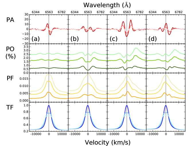
Figure 8: STOKES modelling for a Keplerian rotating scatterer coincident with the location of the disc-like BLR (a), undergoing a vertical outflow (b), a radial outflow (c), and a 45 degree inclined outflow (d). All models consider emission from the central source. From top to bottom, we show the position angle (PA), percentage polarization (PO), polarized flux (PF) and total flux (TF). From darker to lighter shades, the three models shown correspond to viewing angles of 24, 41 and 54 degrees measured from the axis of symmetry of the system.

4 Scatterers in Keplerian rotation

Figure 7, Panel (a), presents a model including Keplerian rotation of the scattering medium for the same parameters presented in Figure 2, Panel (e). As the scatterer is located at larger radii than the BLR, and $v_{\phi}$ goes as the inverse of the square root of the radius, the resulting relative velocity between the two structures is in the same direction as before but with smaller magnitudes. Hence, the scattered line photons present a smaller velocity gradient than in the static configuration. On the other hand, as the scattering region is also rotating with respect to the observer, the photons acquire a further velocity shift after the scattering event. The magnitude of this shift depends on the azimuthal position of the scattering element with respect to the observer. For elements at the near and far side of the scattering region, no shift is introduced as the scatterer is at rest as seen by the observer. Note that these scattering elements, however, contribute little to the scattering signal. For elements at the orthogonal positions, which dominate the observed scattering, the shift is equal to the Keplerian velocity, which corresponds to up to $\sim 2000$ km/s (see Table 1 and discussion below).

Some differences appear at the center of the line when comparing the spectra in Figures 2 Panel (e) and 7 Panel (a), because of the smaller velocity differences between the BLR and scatterer. In particular, the switch in PA values occurs at a smaller velocity range and with larger amplitude, resulting in a sharp swing (see Table 2). At the same time, the wings of the PA profile look more extended because of the velocity shift experienced by the photons at the orthogonal positions: while the W side of the scatterer recedes from us, the E side is approaching us. This also produces small humps in the wings, which are caused by the scattering of the innermost BLR photons: a sharp PA swing at large velocities is produced because of the small subtended angles. This PA shape is smoothed at the orthogonal positions because of the extra velocity shifts, while staying sharp in the signal coming from the near and far sides of the scatterer. The presence (or absence) of these features is therefore dependent on the velocity ranges shown by the BLR and scatterer.

Results are also shown in Figure 7 when including 3000 km/s outflowing ionized material in the vertical ($v_{z}=\pm 3000$ km/s – Panel (b)), radial ($v_{\rho}=3000$ km/s – Panel (c)), and at a 45 degrees ($|v_{z}|=v_{\rho}=3000/\sqrt{2}$ km/s – Panel (d)). Geometric and dynamical constraints can be found in Table 1. When the scatterer presents a net velocity with respect to the BLR two Doppler shifts are involved in any scattering event. The first shift occurs when switching from the reference frame of the BLR (or the previous scattering electron) into the frame of the scattering material. The second occurs after the scattering event, when transforming to the frame of the observer (or the following scattering electron).

The choice of 3000 km/s for the outflowing material is motivated by the velocities reached by the rotating scatterer. For the parameters adopted for this region (Keplerian rotation around a $\sim 10^{7}$ M_☉ black hole with the innermost orbit located at $\sim 0.04$ pc), the equatorial scatterer reaches velocities of $\sim 2000$ km/s. In order for the outflowing component to introduce significant changes its velocity must be of a similar or larger magnitude.

The vertical outflows shown in Figure 7 Panel (b) are launched into both hemispheres, i.e., $v_{z}=\pm 3000$ km/s. To first approximation there is very little net velocity shift between the BLR and the scatterer since the outflowing motion is mostly orthogonal to the BLR motion. This translates into profiles without any net shifts. However, the PA profile becomes complex because the outflow has a component that moves towards us and one that recedes from us, introducing a double swing in the scattering signal and some suppresion in the PA amplitude. Obviously the effects of the outflow are stronger for small inclinations angles, which maximize the velocity outflowing component along the line of sight towards the observer. At larger inclinations the PA profile looks much closer to that seen in Figure 7 Panel (a).

The PF profile in Panel (b) appears broader than in Panel (a) due to the velocity shifts introduced by the outflowing scatterer. The profile presents an enhanced red horn at large viewing angles (54 degrees) and an enhanced blue horn at small viewing angles (24 degrees), but it does not present a net velocity shift as the dynamical configurations from the point of view of the scattering medium and the observer are symmetric which, as we will see, it is not the case with the next model.

Panel (c) in Figure 7 depicts the results from having radial motions. The profiles are clearly shifted redwards as the scatterer is moving away from the BLR in the meridional plane. Also, the effects are stronger than in the case of the vertical outflow because the velocity shifts preferentially occur in the same plane as the travel direction of the scattered photons. The amplitude and sharpness of the PA swing in the less inclined line of sight are both dramatically increased. In the PF spectrum a broad double horn profile of asymmetric intensity appears. Also, the N-S asymmetry discussed in Section 3.2 implies that the redshifted emission from the far side dominates over the near side blushifted emission. This produces a red tail visible beyond 10000 km/s.

Finally, Panel (d) presents the case of a wind outflowing at 45 degrees with respect to the meridional plane of the system. The results are a combination of those already seen in Panels (b) and (c). The PA amplitude variation is suppressed due to the vertical component of the scatterer velocity, while the radial component introduces a redshift to the line features which is smaller than that seen in Panel (c).

S05 also considered the effects of a radial 900 km/s inflowing, non-rotating wind and their results can be compared with our Panel (c) in Figure 7. Other than the obvious net blue-shift in the lines, as the scattering material is inflowing towards the BLR in the S05 models, the main difference with their results is the symmetric peaks in the PF spectra, because S05 considered single scattering events. Also, S05 did not find the strong asymmetric PA profile we see for low inclination angles. This might be due to their outflowing velocity, which is not fast enough to significantly change the velocity structure of the outflowing material.

5 Coincident scattering and emitting regions

A variation of the S05 model has the rotating scattering medium near the BLR location. This could be acieved in two ways.

First, for a thin layer located above and below, sandwiching the BLR region, photons escaping vertically from the emitting material will undergo no scattering, while photons escaping at grazing angles encounter a much larger optical depth and will be scattered. Hence the net PA will be similar to that of the system axis. Second, for a thin scatterer spatially coincident with the BLR region, the same mechanism applies, and a parallel PA is also recovered. These two model realizations (the sandwich and the coincident scatterer) give virtually identical polarization signatures. We present the results corresponding to the coincident scatterer in Figure 8.

Note that the thickness of the BLR has very little impact on our results, but the thinness of the scattering medium is crucial to produce the desired parallel polarization signal. Following S05, a thin BLR has been used in all our models, although it is not clear whether this is a good representation of this structure (see references in the Introduction). For the modelling of a BLR coincident with the scattering region, however, a thin BLR / scatterer geometry must be used since STOKES cannot represent the scatterer as a layer surrounding individual clouds.

Two important differences should be noted in the case of a coincident BLR and scattering region. First, because the scatterer will scatter photons ‘locally’ (i.e., not in rings of scattering material located outside the BLR), there will be no N-S asymmetry due to the large optical depth of the scattering region (see Section 3.1). Second, because the scattering elements will be bombarded by photons coming from all directions, photons coming from directions perpendicular to our line of sight will yield the highest polarization level (see Figure 1), while those approaching the scattering material in directions parallel to our line of sight will give a rather negligible, ‘in transmission’, polarization signal. Before, geometric cancellation happened when combining the signal from opposite regions of the scatterer; now, cancellation will become important at all positions.

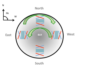
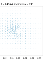
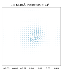
Figure 9: Left: Schematic representation of the position angles seen by elements of the scattering medium for a scatterer coincident with the emitting BLR and in Keplerian rotation. Center and right: PA spatially resolved maps of model 8(a) for wavelengths 6486Å and 6640Å. The sizes of the markers represent the strengths of the polarized fluxes PF and their inclinations represent the PA angles. The axes are expressed in pc.

The scattering events will typically occur when the optical depth of photons reaches a value $\sim 1$. For the electron density assumed in our models this will happen after the photons have travelled about 0.015 pc in a trajectory nearly parallel to the disc mid-plane. This corresponds to $\sim 1/3$ of the disc diameter, which defines the term ‘locally’ used in the previous paragraph. For those photons produced in the innermost regions of the disc scattering will take place in a wide, nearly annular region found at the radius where $\tau\sim 1$, not too differently from the geometry presented in the previous sections. For photons produced in the middle regions of the disc things will differ significantly as they can travel inwards and outwards until they encounter an electron and undergo a scattering event, as discussed further below. Photons produced in the outermost regions of the disc will contribute rather little to the scattering flux as a large fraction of their emission will escape the system. A first approximation, therefore, is to consider only the regions of the BLR found at small and medium radii. In the frame of a scaterrer, due to the Keplerian rotation of the disc, regions at smaller radii will rotate in an anti-clockwise manner, while those at larger radii will rotate in the opposite direction. So approaching and receding photons will be scattered at the same PA irrespective of whether the photon originated at smaller or larger radii. This is schematically shown in the left panel of Figure 9.

At intermediate radii the polarized signal is not produced by photons approaching the scatterer radially, but by those that have travelled a distance such that $\tau\sim 1$, which is satisfied at positions offset from the center. Hence, at the blue side of the line the N region will essentially produce scattering of those photons coming from the W, while the W region will produce scattering of photons coming from the S, and so on, and a swirling pattern will emerge for the polarization signal. At the red side of the line, the pattern will rotate in the opposite direction, as can be seen in Figure 9. These patterns will dissappear as the disc becomes more and more inclined, since photons coming from directions perpendicular to our line of sight will dominate the signal.

In the absence of outflowing motions (Figure 8, Panel (a)) to the previously described effects we only need to add velocity shifts from the rotation of the scatterer as seen by the observer, with the signal from the E side of the disc being blue-shifted while that from the W side of disc is redshifted. The N and S quadrants, on the other hand, present negligible shits, as can be seen in the left panel of Figure 10. Going from shorter to longer wavelengths (from the 6486Å to the 6640Å PA maps presented in Figure 9), the PA signal in the E and W quadrants rotates clockwise, while that in the N and S rotates anticlockwise, as expected. Hence, while the E and W quadrants present a PA profile like the one sketched in Figure 1, the S and N do the opposite, as can be seen in Figure 10. The combined signal corresponds to the central swing seen in the final PA profile, with the regions with the largest polarized flux seen in Figure 9 dominating.

Note the low amplitude variations seen across the line in the PO spectrum in Figure 8 Panel (a), while the PF spectrum is rather narrow and shows very little evidence for a double horn profile. These are the result of the scattering medium having the same Keplerian velocity as the BLR and the scattering elements seeing the photons from approaching and receding BLR regions at very low relative azimuthal velocities.

Models with the same set of outflow velocities previously discussed (vertical, radial and 45 degree inclined) are also shown in 8. Note that the scattering events occur close to the BLR disk despite the different outflowing velocities of the scattering material. In other words, despite the fact that the electrons might be flying away from the BLR, it is only while they belong to a dense thin layer of material that they are able to produce scattering. By not modelling the presence of this wind far away from the BLR, we assume that no further interaction of the photons with these outflowing electrons takes place.

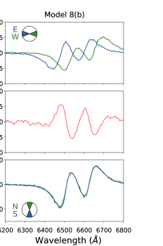
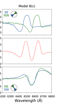
Figure 10: Detailed PA spectra for models presented in Figure 8(a), 8(b) and 8(c). Top and bottom panels show the PA spectra obtained from $\pi/8$ wedge-like regions, as depicted in the pie-charts. The central panels shows in red the total PA spectrum obtained for the full scattering region. For further details see text.

The presence of vertical outflowing motion in the scattering region introduces changes to the polarized spectra as seen in Panel (b). The outflow introduces secondary peaks as the original sinusoidal profiles are blue and red-shifted by the wind (as seen in the center panel of Figure 10), which for small and intermediate disc inclinations – expected for Seyfert I nuclei – will have a significant component along the line of sight to the observer. Rotation will affect the E and W regions to introduce yet another shift, also seen in Figure 10. The PF spectra in Figure 8 look much broader in the presence of a wind, as the approaching and receding velocity components of the outflowing scatterer introduce large Doppler shifts.

Again things appear significantly different when the scattering medium has radial outflows. Figure 8 Panel (c) shows a symmetric, ‘M-shaped’ PA and large amplitude swing which is in stark contrast to Figure 7. The explanation for these new profiles is analogous to that presented earlier for Panels (a) and (b).

In the rest frame of the scattering elements, there will be large velocity offsets with respect to the emitting BLR due to the radial outflow. At each location the PA profile will combine the blue-shifted swing from the BLR located at larger radii with a red-shifted swing from the BLR located at smaller radii. A combined PA profile corresponding to a complete back-and-forth rotation will emerge.

To further understand this case it is best to split the scatterer into NE-NW-SE-SW regions. As seen by the observer, the combination of the radial outflow and the rotation motion will give NW and SE regions receding and approaching, respectively, while the NE and SW regions will remain largely at rest. Hence the SE and NW PA profiles will get pushed blue and red-wards, respectively, as can be seen in right panel of Figure 10, while the NE and SW profiles stay at the rest line velocity. Back-and-forth PA rotations will occur in a clockwise followed by an anti-clockwise manner for the NW and SE regions, while an anti-clockwise rotation followed by a clockwise rotation will occur at the NE and SW regions, as seen in Figure 10. The final combination of all regions gives a very symmetric M-shaped PA profile.

Note that, as before, projection effects will affect all velocity components in the same way, and therefore the emerging profile is symmetric in velocity space. The only differences would appear because of possible boosting effects along the line of sight. However, as all velocity fields are contained in the plane of the disc, and in Seyfert I nuclei this inclination angle of the disc is usually small, boosting should not be significant for this case.

Panel (d) presents the case for a 45 degree outflow. In this case, the features already seen in cases (b) and (c) play a role. The final PA profile is complex and asymmetric.

6 Discussion

6.1 General results

Using state of the art Monte Carlo STOKES simulations we have been able to recover and extend the work done by S05 on the polarized signal of broad emission lines in Type I AGN. Our treatment finds similar results to those published by S05, but requires some significant changes to the S05 original set up, as discussed in Section 3. We found that the final scattering signal cannot be based solely on emission from the orthogonal sides of the scatterer; emission from the near and far sides must be included to find the correct polarized signal. As a result, our treatment yields a reverse PA swing to that originally proposed. Also, a much larger optical depth (up by one order of magnitude) is required to obtain significant levels of polarization (a few %), and a much thicker equatorial scatterer is needed to recover the emission line PA swing discussed at length by S05.

Marin et al. (2012, 2013) also found that large optical depths ($\tau\sim 1-3$) are necessary to obtain the level of polarization usually seen in AGN. Using STOKES to model the phenomenologically motivated central source structure proposed by Elvis (2000), Marin et al. showed that an outflowing electron scatterer will yield polarization of a few percent if the wind is optically thick to electron scattering.

We have included the presence of the central continuum emitting source as part of our modelling, which clearly represents a more accurate prescription of the scattering signal. The inclusion of large (3000 km/s) bulk motion due to an outflowing scatterer shows that the scattering signal can deviate significantly from the S05 predictions, yielding new profiles that can be readily tested against observations.

We also explored a new configuration for the BLR and scatterer regions where they are spatially coincident, either with the scatterer acting as an ‘atmosphere’ for the BLR or fully mixed with it. The results from this new configuration give very different results when outflows are considered, with an M-shaped PA profile being predicted as a result of the scattering of photons undergoing symmetric shifts from the wind and rotational fields. This M-like signal is a clear indication of the scattering taking place in a cospatial BLR and equatorial outflow and has already been observed in spectropolarimetric observations of nearby Seyfert galaxies, as discussed below.

6.2 Qualitative comparison with observations

High signal-to-noise ratio spectropolarimetric observations of Seyfert I galaxies have become available in recent years (e.g., Afanasiev et al. 2019). Some of the observations show rich PA profiles that could not be explained by the S05 results: NGC 3783 spectropolarimetric observations do not present the usual sinusoidal swing, but a deep M-like shaped morphology instead (Lira et al. 2007). We believe the observed profile can be explained by the cospatial nature of the BLR and an outflowing equatorial scatterer. Detailed simulation of these sources is left to a future paper.

References

- Afanasiev, Popović & Shapovalova (2019) Afanasiev V. L., Popović L. Č., Shapovalova A. I., 2019, MNRAS, 482, 4985
- Antonucci (1993) Antonucci R., 1993, ARA&A, 31, 473
- Brown & McLean (1977) Brown J. C., McLean I. S., 1977, A&A, 57, 141
- Chiang & Murray (1996) Chiang J., Murray N., 1996, ApJ, 466, 704
- Collin-Souffrin, Dyson, McDowell & Perry (1988) Collin-Souffrin S., Dyson J. E., McDowell J. C., Perry J. J., 1988, MNRAS, 232, 539
- Elvis (2000) Elvis M., 2000, ApJ, 545, 63
- Eracleous & Halpern (2003) Eracleous M., Halpern J. P., 2003, ApJ, 599, 886
- Eracleous & Halpern (1994) Eracleous M., Halpern J. P., 1994, ApJS, 90, 1
- Goodrich (1989) Goodrich R. W., 1989, ApJ, 342, 224
- Goosmann & Gaskell (2007) Goosmann R. W., Gaskell C. M., 2007, A&A, 465, 129
- Kollatschny (2003) Kollatschny W., 2003, A&A, 407, 461
- Lira, et al. (2007) Lira P., et al., 2007, ASPC..373, 407, ASPC..373
- Marin, Goosmann, Gaskell, Porquet & Dovčiak (2012) Marin F., Goosmann R. W., Gaskell C. M., Porquet D., Dovčiak M., 2012, A&A, 548, A121
- Marin & Goosmann (2013) Marin F., Goosmann R. W., 2013, MNRAS, 436, 2522
- Mejía-Restrepo, Lira, Netzer, Trakhtenbrot & Capellupo (2018) Mejía-Restrepo J. E., Lira P., Netzer H., Trakhtenbrot B., Capellupo D. M., 2018, NatAs, 2, 63
- Marziani, Sulentic, Dultzin-Hacyan, Calvani & Moles (1996) Marziani P., Sulentic J. W., Dultzin-Hacyan D., Calvani M., Moles M., 1996, ApJS, 104, 37
- Murray & Chiang (1997) Murray N., Chiang J., 1997, ApJ, 474, 91
- Pancoast, Brewer, Treu, Park, Barth, Bentz & Woo (2014) Pancoast A., Brewer B. J., Treu T., Park D., Barth A. J., Bentz M. C., Woo J.-H., 2014, MNRAS, 445, 3073
- Proga & Kurosawa (2010) Proga D., Kurosawa R., 2010, Accretion and Ejection in AGN: a Global View, 41, ASPC..427
- Runnoe, Brotherton, Shang, Wills & DiPompeo (2013) Runnoe J. C., Brotherton M. S., Shang Z., Wills B. J., DiPompeo M. A., 2013, MNRAS, 429, 135
- Savić, Goosmann, Popović, Marin & Afanasiev (2018) Savić D., Goosmann R., Popović L. Č., Marin F., Afanasiev V. L., 2018, A&A, 614, A120
- Schmid, Appenzeller, Camenzind, Dietrich, Heidt, Schild & Wagner (2001) Schmid H. M., Appenzeller I., Camenzind M., Dietrich M., Heidt J., Schild H., Wagner S., 2001, A&A, 372, 59
- Shakhovskoi (1965) Shakhovskoi N. M., 1965, SvA, 8, 833
- Shen & Ho (2014) Shen Y., Ho L. C., 2014, Natur, 513, 210
- Smith, Robinson, Young, Axon & Corbett (2005) Smith J. E., Robinson A., Young S., Axon D. J., Corbett E. A., 2005, MNRAS, 359, 846
- Smith, Robinson, Alexander, Young, Axon & Corbett (2004) Smith J. E., Robinson A., Alexander D. M., Young S., Axon D. J., Corbett E. A., 2004, MNRAS, 350, 140
- Smith, Young, Robinson, Corbett, Giannuzzo, Axon & Hough (2002) Smith J. E., Young S., Robinson A., Corbett E. A., Giannuzzo M. E., Axon D. J., Hough J. H., 2002, MNRAS, 335, 773
- Smith, Schmidt, Allen & Hines (1997) Smith P. S., Schmidt G. D., Allen R. G., Hines D. C., 1997, ApJ, 488, 202
- Gravity Collaboration, et al. (2018) Gravity Collaboration, et al., 2018, Natur, 563, 657
- Wills & Browne (1986) Wills B. J., Browne I. W. A., 1986, ApJ, 302, 56
- Wood, Brown & Fox (1993) Wood K., Brown J. C., Fox G. K., 1993, A&A, 271, 492