Time-sliced perturbation theory with primordial non-Gaussianity and effects of large bulk flows on inflationary oscillating features

Abstract

We extend the formalism of time-sliced perturbation theory (TSPT) for cosmological large-scale structure to include non-Gaussian initial conditions. We show that in such a case the TSPT interaction vertices acquire new contributions whose time-dependence factorizes for the Einstein-de Sitter cosmology. The new formulation is free from spurious infrared (IR) enhancements and reveals a clear IR structure of non-Gaussian vertices. We use the new technique to study the evolution of oscillating features in primordial statistics and show that they are damped due to non-linear effects of large bulk flows. We derive the damping factors for the oscillating primordial power spectrum and bispectrum by means of a systematic IR resummation of relevant Feynman diagrams.

1 Introduction

Large scale structure (LSS) provides us with a powerful tool to study the dynamical and statistical properties of our universe. This structure has been formed during the epoch of matter domination and its dynamics on large scales is governed by dark matter and baryons acting as single pressureless perfect fluids. The three-dimensional distribution of LSS can potentially supersede the cosmic microwave background (CMB) measurements in the number of Fourier modes available for observations. On the other hand, the relevant cosmological information encoded in LSS is concealed by the non-linear effects related to gravitational clustering. Disentangling the cosmological information from these effects presents a highly non-trivial challenge that must be addressed in order to efficiently use the data of the ongoing and future surveys.

The standard tool to model dark matter clustering in the non-linear regime is N-body simulations, which are progressively becoming more robust and accessible. On the other hand, reaching the accuracy level required by future surveys still remains computationally expensive [1]. Besides, implementing non-minimal cosmological scenarios or initial conditions (e.g. primordial non-Gaussianity) still requires non-trivial extensions of the standard N-body codes.

An alternative way is the development of analytic methods based on perturbation theory [2]. Although limited to a range of large scales, this approach has a number of advantages. First, analytic methods allow for a shorter computational time. Second, they give valuable insights into the physics of non-linear clustering. Third, they are flexible and can be easily extended to models beyond the standard $\Lambda$CDM cosmology.

One of the goals of future LSS surveys is probing primordial non-Gaussianity (PNG), which can shed light on the dynamics of inflation or its alternatives. This task is complicated by a number of factors. First, generic non-Gaussian phenomena are encoded in higher-order statistics, which are hard to measure and interpret. Second, the primordial non-Gaussian signal must be disentangled from that generated by non-linear gravitational instability even from initially Gaussian fields. Perturbation theory provides a natural and computationally efficient way to do this [3]. Perturbative calculations including primordial non-Gaussianity were performed for the power spectrum [4] and bispectrum [5] of matter and biased tracers. The analysis of galaxy bias was later refined in [6], see [7] for a review. The Effective Field Theory (EFT) of LSS [8, 9] has been applied to compute the power spectrum and bispectrum with non-Gaussian initial conditions [10]. Based on these developments, an analysis of the ability to extract the PNG signal from LSS was carried out in [12, 11, 15, 13, 14].

A particularly interesting question is existence of oscillatory features in the statistics of primordial density fluctuations. Such resonance features naturally appear in models inspired by the axion monodromy inflation [16] where the inflaton potential is modulated by small sinusoidal oscillations [17, 18]. Alternatively, they can be generated by the interaction between the inflaton and massive particles, thereby encoding information about the particle spectrum at inflation [19, 20, 21]. The latter type of non-Gaussianity has got the name of cosmological collider signatures.

Oscillating features in the primordial power spectrum have been constrained from the CMB data by the Planck collaboration [22, 23]. The prospects to improve these constraints using future LSS and 21 cm surveys were studied in [24, 25, 26, 27, 28], see also the recent white paper [29] and references therein. The Planck collaboration has also performed searches for oscillating primordial non-Gaussianity in CMB with the null results [30]. The imprint of resonant non-Gaussianity on the scale dependent halo bias was discussed in [31], whereas Ref. [28] analyzed the sensitivity of 21 cm intensity mapping to this type of PNG. Refs. [32, 33] presented forecasts for the reach of LSS and 21 cm surveys in probing cosmological collider signatures. As pointed out in Ref. [34], one expects primordial oscillations in LSS statistics to get damped at late times due to the non-linear effects of large bulk flows, similarly to the damping of baryon acoustic oscillations (BAO). Indeed, the displacement of modes with Fourier momentum $k$ caused by non-linear coupling to long modes with momentum $q\ll k$ washes out the features with a characteristic period of oscillations in Fourier space $k_{osc}\ll q$ smaller that the long-mode momentum. However, this effect was not discussed beyond the power spectrum.

In this paper we study the non-linear damping of primordial oscillations in the inflationary 3-point function (bispectrum). We work out a systematic procedure of infrared (IR) resummation that captures the effect of large bulk flows. Our method is inspired by techniques developed in the context of the BAO and is based on Time-Sliced Perturbation Theory (TSPT) [35]. The latter has been proven to be a powerful tool for IR resummation of the power spectrum and higher-order statistics [36, 37].

TSPT is a novel way of performing cosmological perturbation theory utilizing the machinery of quantum field theory and statistical physics. The key idea of this method is to study the time-dependent probability distribution function of density and velocity fields, instead of these fields themselves as done in the standard cosmological perturbations theory (SPT). The central object is the generating functional for cosmological correlators whose time evolution is governed by a Liouville equation of statistical mechanics. A perturbative expansion of the generating functional leads to Feynman rules similar to that of a 3-dimensional Euclidean quantum field theory, in which time plays a role of an external parameter. This expansion produces equal-time correlation functions of density and velocity at fixed time (redshift) slices, which explains the name to the method.

TSPT deals directly with the statistical quantities, such as equal time n-point correlation functions, and thus provides a natural framework for studying non-Gaussian initial conditions. We will show that the incorporation of such conditions is straightforward and results in new contributions to the TSPT vertices. The new contributions take particularly simple form for the Einstein-de Sitter (EdS) cosmology, where time dependence of the TSPT vertices factors out. We introduce a new convenient diagrammatic technique for the primordial non-Gaussian contributions. As suggested by observations, the latter should be treated as small perturbations on top of the standard correlation function corresponding to Gaussian initial conditions. The eventual expressions for TSPT correlation functions at fixed order of perturbation theory coincide with the SPT result, although the individual diagrams are quite different. In particular, we will show that the non-Gaussian TSPT vertices do not contain any singularities originating from dynamical non-linear mode-coupling. In this sense they are IR-safe. Of course, they may still contain physical IR singularities which may be contained in the primordial statistics themselves.

Finally, we show how the new reformulation allows for a systematic IR resummation of the large bulk flow effects on the evolution of oscillatory primordial statistics. We show that IR resummation in this case closely resembles that of the BAO for the Gaussian initial statistics and leads to a smearing of oscillating features. In particular, the relevant contributions to be resummed have a graphical representation of daisy diagrams. We derive explicit expressions for the non-linear damping factors of the power spectrum and bispectrum. In the latter case the damping depends on the full configuration of the wavevectors, including their relative angles.

The paper is organized as follows. In Sec. 2 we set up conventions and discuss the standard treatment of non-Gaussian initial conditions in cosmological perturbation theory. In Sec. 3 we recapitulate the Gaussian TSPT framework. In Sec. 4 we extend it by including the non-Gaussian initial conditions. Section 5 contains the proof of the IR safety of the non-Gaussian TSPT vertices. In Sec. 6 we present a framework for IR resummation of non-Gaussian vertices and apply it to the non-linear evolution of the resonant power spectrum and bispectrum from axion monodromy inflation. We conclude in Sec. 7. Some additional material is given in Appendices.

In the numerical calculations throughout the paper we use the Planck 2018 cosmology [38] with massless neutrinos. The linear power spectrum is computed with the Boltzmann code CLASS [39].

2 Preliminaries

In this section we set up the conventions and discuss the standard treatment of non-Gaussian initial conditions in LSS. Throughout the paper we will mostly focus on the non-trivial initial 3-point function (bispectrum). However, our results can be straightforwardly generalized to the case of higher non-Gaussian statistics. We will comment on this point at the relevant places in the text.

2.1 Primordial and linear statistics

We will distinguish between primordial and linear bispectra. We adopt the inflationary paradigm and call primordial the quantities referring to the curvature perturbation $\zeta$ generated during inflation. Its statistical properties are encoded in the power spectrum and the bispectrum,

$$\langle\zeta({\bf k})\zeta({\bf k}^{\prime})\rangle=(2\pi)^{3}\delta^{(3)}_{D}({\bf k}+{\bf k}^{\prime})P_{\zeta}(k)\,,$$ (2.1a)

$$\langle\zeta({\bf k}_{1})\zeta({\bf k}_{2})\zeta({\bf k}_{3})\rangle=(2\pi)^{3}\delta^{(3)}_{D}({\bf k}_{1}+{\bf k}_{2}+{\bf k}_{3})B_{\zeta}({\bf k}_{1},{\bf k}_{2},{\bf k}_{3})\,,$$ (2.1b)

where $\delta^{(3)}_{D}$ is the 3-dimensional Dirac delta-function. The power spectrum of the primordial curvature perturbations can be written as,

$$P_{\zeta}(k)\equiv\frac{\mathcal{A}^{2}_{\zeta}}{k^{3}}\left(\frac{k}{k_{*}}\right)^{n_{s}-1}\,,$$ (2.2)

where $k_{*}$ is a pivot scale, $\mathcal{A}^{2}_{\zeta}$ is the amplitude and $(n_{s}-1)$ is the tilt of the spectrum. Their mean values from the latest Planck CMB temperature and polarization measurements [38] for $k_{*}=0.05\,$Mpc^-1 are

$$\mathcal{A}^{2}_{\zeta}=4.14\cdot 10^{-8}\;,~{}~{}~{}~{}~{}~{}~{}n_{s}=0.965\,.$$ (2.3)

Let us outline some properties of $B_{\zeta}({\bf k}_{1},{\bf k}_{2},{\bf k}_{3})$ in typical inflationary models, see Ref. [40] for more details. Due to momentum conservation and rotational invariance the bispectrum is a function of three independent variables only. These can be chosen to be either the three momenta norms $k_{1},k_{2},k_{3}$, or the norms of a pair of momenta, say $k_{1},k_{2}$, and the cosine $\mu_{12}$ of the angle between them. Approximate scale invariance implies that $B_{\zeta}$ is a homogeneous function of degree $-6$, symmetric in its arguments. The shapes commonly used in data analysis are local [41], equilateral [42], and orthogonal [43],

$$B^{\text{loc}.}_{\zeta}(k_{1},k_{2},k_{3})=\frac{6}{5}f_{NL}^{\text{loc}.}\Big{(}P_{\zeta}(k_{1})P_{\zeta}(k_{2})+P_{\zeta}(k_{2})P_{\zeta}(k_{3})+P_{\zeta}(k_{3})P_{\zeta}(k_{1})\Big{)}\,,$$ (2.4a)

$$B^{\text{eq}.}_{\zeta}(k_{1},k_{2},k_{3})=\frac{18}{5}f_{NL}^{\text{eq}.}\mathcal{A}_{\zeta}^{4}\left(-\frac{1}{k_{1}^{3}k_{2}^{3}}-\frac{1}{k_{2}^{3}k_{3}^{3}}-\frac{1}{k_{3}^{3}k_{1}^{3}}-\frac{2}{k_{1}^{2}k_{2}^{2}k_{3}^{2}}+\sum_{i\neq j\neq l}\frac{1}{k_{i}k_{j}^{2}k_{l}^{3}}\right),$$ (2.4b)

$$B^{\text{orth}.}_{\zeta}(k_{1},k_{2},k_{3})=\frac{18}{5}f_{NL}^{\text{orth}.}\mathcal{A}_{\zeta}^{4}\left(\!-\frac{3}{k_{1}^{3}k_{2}^{3}}\!-\!\frac{3}{k_{2}^{3}k_{3}^{3}}\!-\!\frac{3}{k_{3}^{3}k_{1}^{3}}\!-\!\frac{8}{k_{1}^{2}k_{2}^{2}k_{3}^{2}}\!+3\!\!\sum_{i\neq j\neq l}\frac{1}{k_{i}k_{j}^{2}k_{l}^{3}}\!\right),$$ (2.4c)

where in the last two expressions we for simplicity neglected the departures from scale invariance (the tilt). The current observational constraints on $f_{NL}$ (at $68\%$ CL) from the CMB measurements are [30],

$$f^{\text{loc}.}_{NL}=-0.9\pm 5.1\,,\qquad f^{\text{eq}.}_{NL}=-26\pm 47\,,\qquad f^{\text{orth}.}_{NL}=-38\pm 24\,.$$ (2.5)

The key objects for the description of LSS are the matter density contrast $\delta=(\rho-\bar{\rho})/\bar{\rho}$ and velocity divergence $\Theta\propto\nabla\cdot{\bm{u}}$ fields. Here $\bar{\rho}$ is the average density of the Universe and ${\bm{u}}$ is the peculiar flow velocity. Initially small, these fields start growing after recombination and become non-linear. This non-linear evolution is captured by the cosmological perturbation theory, which uses as a seed the linear fields $\delta_{L}$, $\Theta_{L}$ evolved up to the present epoch as if the perturbations were always in the linear regime. In the case of adiabatic initial conditions corresponding to a growing mode the two linear fields are identical. They are related to the curvature perturbation $\zeta$ by a transfer function $T(t_{0};{\bf k})$ which encodes the evolution of perturbations from inflation, through recombination, up to the present time $t_{0}$. Thus we write,

$$\Theta_{L}({\bf k})=\delta_{L}({\bf k})\equiv T(t_{0};{\bf k})\zeta({\bf k})\,.$$ (2.6)

We will understand by linear statistics the properties of the field $\delta_{L}$. Defining the linear matter power spectrum,

$$\langle\delta_{L}({\bf k})\delta_{L}({\bf k}^{\prime})\rangle=(2\pi)^{3}\delta^{(3)}_{D}({\bf k}+{\bf k}^{\prime})P_{L}(k)\;,$$ (2.7)

we see that

$$P_{L}(k)=[T(t_{0};k)]^{2}P_{\zeta}(k)\;.$$ (2.8)

From this we immediately deduce the relation between the linear bispectrum of LSS and the primordial one,

$$\begin{split}B_{L}(k_{1},k_{2},k_{3})=&\sqrt{\frac{P_{L}(k_{1})}{P_{\zeta}(k_{1})}\frac{P_{L}(k_{2})}{P_{\zeta}(k_{2})}\frac{P_{L}(k_{3})}{P_{\zeta}(k_{3})}}B_{\zeta}(k_{1},k_{2},k_{3})\,.\end{split}$$ (2.9)

Note that the linear bispectrum is parametrically suppressed by the amplitude of the primordial fluctuations. Indeed, neglecting the shape of the bispectrum one has, schematically,

$$\frac{\langle\delta_{L}^{3}\rangle}{(\langle\delta_{L}^{2}\rangle)^{3/2}}\sim\frac{B_{L}}{(P_{L})^{3/2}}\sim f_{NL}\mathcal{A}_{\zeta}\ll 1\,.$$ (2.10)

The linear power spectrum (2.8) and bispectrum (2.9) serve as the input for the equations describing the non-linear evolution of LSS statistics at times after recombination.

2.2 Standard perturbation theory with non-Gaussian initial conditions

We are interested in the correlation functions of the overdensity and the velocity divergence fields, whose time-evolution is governed by the following pressureless perfect fluid equations:

$$\frac{\partial\delta}{\partial t}+\nabla\cdot[(1+\delta){\bm{u}}]=0\,,$$ (2.11a)

$$\frac{\partial{\bm{u}}}{\partial t}+{\cal H}{\bm{u}}+({\bm{u}}\cdot\nabla){\bm{u}}=-\nabla\phi\,,$$ (2.11b)

where $\phi$ is the gravitational potential obeying the Poisson equation,

$$\nabla^{2}\phi=\frac{3}{2}{\cal H}^{2}\Omega_{m}\delta\,.$$ (2.12)

Here $t$ is the conformal time, the spatial derivatives are taken with respect to the comoving coordinates, ${\cal H}=aH$ is the rescaled Hubble parameter, $a$ is the scale factor and $\Omega_{m}$ is the matter density fraction.

The single-stream perfect fluid approximation breaks down at short scales due to free-streaming of dark matter particles (also called ‘shell-crossing’). These effects show up when one computes loop contributions generated by hard modes. They are taken into account in the EFT of LSS, where the influence of short scale nonlinearities on physics at large scales is encapsulated by an effective stress tensor added to the r.h.s. of (2.11) [8, 9]. For simplicity, we do not explicitly consider the EFT corrections in this paper, keeping in mind that eventually they will have to be properly included. The main goal of this paper is to study the non-linear effects of very long-wavelength (IR) modes, for which the perfect fluid description is sufficient.

It is well-known [2] that in the case of an EdS universe dominated by non-relativistic matter ($\Omega_{m}=1$) the above equations can be cast in a form free from any explicit time dependence. This is achieved by introducing the time parameter

$$\eta=\mathop{\rm ln}\nolimits D(t)\;,$$ (2.13)

where $D$ is the linear growth factor, and appropriately rescaling the velocity divergence,

$$\Theta=-\frac{\nabla\cdot{\bm{u}}}{{\cal H}f}~{},\qquad\text{with}~{}f=\frac{d\mathop{\rm ln}\nolimits D}{d\mathop{\rm ln}\nolimits a}\;.$$ (2.14)

For the realistic $\Lambda$CDM cosmology, the above substitution leaves a small residual time dependence which, however, has little effect on the dynamics [44]. Following conventional practice we will neglect this explicit time dependence in the equations, even though our analysis does not crucially depend on this restriction.

Within the above approximation Eqs. (2.11) can be rewritten in Fourier space as

$$\partial_{\eta}\delta_{\bf k}-\Theta_{\bf k}=\int[dq]^{2}\,(2\pi)^{3}\delta^{(3)}_{D}({\bf k}-{\bf q}_{12})\alpha({\bf q}_{1},{\bf q}_{2})\Theta_{{\bf q}_{1}}\delta_{{\bf q}_{2}}\,,$$ (2.15a)

$$\partial_{\eta}\Theta_{\bf k}+\frac{1}{2}\Theta_{\bf k}-\frac{3}{2}\delta_{\bf k}=\int[dq]^{2}\,(2\pi)^{3}\delta^{(3)}_{D}({\bf k}-{\bf q}_{12})\beta({\bf q}_{1},{\bf q}_{2})\Theta_{{\bf q}_{1}}\Theta_{{\bf q}_{2}}\,,$$ (2.15b)

where we used the notations,

$$[dq]^{n}\equiv\frac{d^{3}q_{1}...d^{3}q_{n}}{(2\pi)^{3n}}\,,\quad\quad{\bf q}_{1...n}={\bf q}_{1}+...+{\bf q}_{n}\,,$$

and introduced the non-linear kernels

$$\alpha({\bf k}_{1},{\bf k}_{2})\equiv\frac{({\bf k}_{1}+{\bf k}_{2})\cdot{\bf k}_{1}}{k_{1}^{2}}\,,\quad\quad\beta({\bf k}_{1},{\bf k}_{2})\equiv\frac{({\bf k}_{1}+{\bf k}_{2})^{2}({\bf k}_{1}\cdot{\bf k}_{2})}{2k_{1}^{2}k_{2}^{2}}\,.$$ (2.16)

These equations can be solved perturbatively by using the following power series Ansatz:

$$\delta_{\bf k}=\sum_{n=1}^{\infty}\big{(}D(\eta)\big{)}^{n}\int[dq]^{n}\,(2\pi)^{3}\delta^{(3)}_{D}({\bf k}-{\bf q}_{1...n})F_{n}({\bf q}_{1},...,{\bf q}_{n})\delta_{L}({\bf q}_{1})...\delta_{L}({\bf q}_{n})\,,$$ (2.17a)

$$\Theta_{\bf k}=\sum_{n=1}^{\infty}\big{(}D(\eta)\big{)}^{n}\int[dq]^{n}\,(2\pi)^{3}\delta^{(3)}_{D}({\bf k}-{\bf q}_{1...n})G_{n}({\bf q}_{1},...,{\bf q}_{n})\delta_{L}({\bf q}_{1})...\delta_{L}({\bf q}_{n})\,,$$ (2.17b)

where $\delta_{L}$ is the linear density field and the non-linear kernels $F_{n}$ and $G_{n}$ are recursively derived from (2.15). The correlation functions of the fields $\delta_{\bf k}$, $\Theta_{\bf k}$ are computed by averaging the expressions (2.17) using the statistics of the linear field $\delta_{L}$. The resulting expressions are conveniently represented as diagrammatic expansions in the number of loops. This method is known as Eulerian standard perturbation theory (SPT) [2]. Typically, the linear statistics are assumed to be Gaussian and adiabatic, i.e. they are fully characterized by the power spectrum (2.7). Recall that the initial conditions for structure formation are set shortly after recombination when baryons and dark matter started to behave as a single pressureless fluid, but the gravitational instability did not yet have enough time to form non-linear structures. For simplicity, we neglect non-Gaussianity generated by the second order effects at radiation domination and recombination [45, 46, 47].

Suppose now that in addition to the power spectrum the linear distribution of the density contrast is also characterized by a non-trivial 3-point function,

$$\begin{split}&\langle\delta_{L}({\bf k}_{1})\delta_{L}({\bf k}_{2})\delta_{L}({\bf k}_{3})\rangle=(2\pi)^{3}\delta^{(3)}_{D}({\bf k}_{1}+{\bf k}_{2}+{\bf k}_{3})B_{L}(k_{1},k_{2},k_{3})\,.\end{split}$$ (2.18)

This generates additional terms in the SPT perturbative expansion, which originate from averages of odd number of fields. For instance, the leading-order (tree-level) matter bispectrum and the 1-loop correction to the matter power spectrum read,

$$B_{\rm SPT}^{\rm tree}(\eta;k_{1},k_{2},k_{3})=2\big{(}D(\eta)\big{)}^{4}\sum_{1\leq i<j\leq 3}F_{2}({\bf k}_{i},{\bf k}_{j})P_{L}(k_{i})P_{L}(k_{j})+\big{(}D(\eta)\big{)}^{3}B_{L}(k_{1},k_{2},k_{3})\,,$$ (2.19a)

$$P_{\text{SPT}}^{\text{1-loop}}(\eta;k)=\big{(}D(\eta)\big{)}^{4}\bigg{(}2\int[dq]P_{L}(q)P_{L}(|{\bf k}-{\bf q}|)\big{(}F_{2}({\bf q},{\bf k}-{\bf q})\big{)}^{2}$$

$$\qquad+6P_{L}(k)\int[dq]P_{L}(q)F_{3}({\bf k},{\bf q},-{\bf q})\bigg{)}+2\big{(}D(\eta)\big{)}^{3}\int[dq]B_{L}(q,|{\bf k}-{\bf q}|,k)F_{2}({\bf q},{\bf k}-{\bf q})\,.$$ (2.19b)

Note that the primordial non-Gaussian contributions have one less power of the growth factor $D(\eta)$ compared to the terms coming from the non-linear evolution.

Let us discuss an important point. The kernels $\alpha$ and $\beta$ entering the Euler equations have poles if one of their arguments vanishes, see Eqs. (2.16). These IR singularities are inherited by the non-linear kernels $F_{n}$, $G_{n}$; for example,

$$F_{2}({\bf k},{\bf q})\Big{|}_{|{\bf q}|\to 0}\simeq\frac{{\bf k}\cdot{\bf q}}{2q^{2}}\;.$$

This leads, in turn, to IR poles in the integrands of the loop expressions. The origin of the IR singularities can be traced back to large displacements of short-wavelength density perturbations by long-wavelength bulk flows. This effect should, however, cancel in the correlation functions of fields taken at the same moment of time. Indeed, the cancellation of IR singularities in equal-time correlators is a well-known property in Gaussian SPT, see [48] and references therein. For non-Gaussian initial conditions, the cancellation of contributions due to the IR poles can be tracked explicitly at the lowest orders of the perturbation theory; however, we are not aware of a general proof in the literature. Clearly, it is desirable to have a framework where spurious IR singularities are absent altogether. Such framework is provided by the time-sliced perturbation theory [35] described in the subsequent sections.

It is important to stress that the IR poles discussed above should be distinguished from those that may be present in the primordial bispectrum itself and thus are physical. Throughout the paper ‘IR poles’ or ‘IR singularities’ will only refer to the singularities originated from the non-linear mode coupling.

3 Review of Gaussian TSPT

The main idea of the TSPT approach is to substitute the time evolution of the overdensity and velocity divergence fields, $\delta$ and $\Theta$, by that of the their time dependent probability distribution functional (PDF). This idea is natural when one is only interested in equal time correlation functions. For adiabatic initial conditions only one of the two fields is statistically independent. It is convenient to choose the velocity divergence field $\Theta$ as an independent variable and its PDF will be denoted by $\mathcal{P}[\Theta;\eta]$. At any moment in time, the field $\delta$ can be expressed in terms of $\Theta$ as

$$\delta({\bf k})\equiv\delta[\Theta;\eta,{\bf k}]=\sum_{n=1}^{\infty}\frac{1}{n!}\int[dq]^{n}(2\pi)^{3}\delta^{(3)}_{D}\big{(}{\bf k}-{\bf q}_{1\ldots n}\big{)}\,K_{n}(\eta;{\bf q}_{1},...,{\bf q}_{n})\prod_{j=1}^{n}\Theta({\bf q}_{j})\,.$$ (3.1)

Note that, in contrast to the SPT formulae (2.17), we have here on the r.h.s. the full non-linear field $\Theta({\bf q})$. Recursion relations for the kernels $K_{n}$ are given in Appendix A. Equation (3.1) can be used to eliminate the density field from Eq. (2.15b) and obtain the following equation for the velocity divergence,

$$\dot{\Theta}({\bf k})=\mathcal{I}[\Theta;\eta]\equiv\sum_{n=1}^{\infty}\frac{1}{n!}\int[dq]^{n}(2\pi)^{3}\delta^{(3)}_{D}\big{(}{\bf k}-{\bf q}_{1\ldots n}\big{)}\,I_{n}(\eta;{\bf q}_{1},...,{\bf q}_{n})\prod_{j=1}^{n}\Theta({\bf q}_{j})\,,$$ (3.2)

with $I_{1}\equiv 1$ corresponding to the adiabatic mode in the perfect fluid approximation. The other kernels $I_{n}$ can be derived from the fluid equations (2.15), see Appendix A. In the EdS approximation both kernels $K_{n}$ and $I_{n}$ are time independent.

One introduces the generating functional,

$$Z[J,J_{\delta};\eta]=\int[\mathcal{D}\Theta]\;{\mathcal{P}}[\Theta;\eta]\;\exp\bigg{\{}\int[dk]\Theta({\bf k})J(-{\bf k})+\int[dk]\delta[\Theta;\eta,{\bf k}]J_{\delta}(-{\bf k})\bigg{\}}\,.$$ (3.3)

Equal-time correlation functions for $\Theta$ and $\delta$ are obtained by taking functional derivatives of $Z$ with respect to the external sources $J$ or $J_{\delta}$, respectively. For example, the matter power spectrum is given by

$$(2\pi)^{3}\delta^{(3)}_{D}({\bf k}+{\bf k}^{\prime})\,P(\eta;k)=\frac{\delta^{2}Z}{\delta J_{\delta}(-{\bf k})\delta J_{\delta}(-{\bf k}^{\prime})}\bigg{|}_{J=J_{\delta}=0}\,.$$ (3.4)

The conservation of probability implies the Liouville equation for the probability density functional,

$$\frac{\partial}{\partial\eta}\mathcal{P}[\Theta;\eta]+\int[dk]\frac{\delta}{\delta\Theta({\bf k})}\big{(}\mathcal{I}[\Theta;\eta]\mathcal{P}[\Theta;\eta]\big{)}=0\,.$$ (3.5)

It is useful to expand $\mathop{\rm ln}\nolimits\mathcal{P}[\Theta;\eta]$ as a power series in $\Theta$,

$$\mathcal{P}[\Theta;\eta]=\mathcal{N}^{-1}\exp\Bigg{\{}-\sum_{n=1}^{\infty}\frac{1}{n!}\int[dk]^{n}\;\Gamma_{n}^{tot}(\eta;{\bf k}_{1},...,{\bf k}_{n})\;\prod^{n}_{j=1}\Theta({\bf k}_{j})\Bigg{\}}\,,$$ (3.6)

where ${\cal N}$ is a normalization factor. Then, using Eq. (3.2) we obtain the following chain of equations for the vertices $\Gamma^{tot}_{n}$,

$$\begin{split}&\dot{\Gamma}_{n}^{tot}(\eta;{\bf k}_{1},...,{\bf k}_{n})+\sum_{m=1}^{n}\sum_{\sigma}\frac{I_{m}(\eta;{\bf k}_{\sigma(1)},...,{\bf k}_{\sigma(m)})}{m!(n-m)!}\,\Gamma_{n-m+1}^{tot}\bigg{(}\eta;\sum_{i=1}^{m}{\bf k}_{\sigma(i)},{\bf k}_{\sigma(m+1)},...,{\bf k}_{\sigma(n)}\bigg{)}\\ &=(2\pi)^{3}\delta^{(3)}_{D}\left({\bf k}_{1\ldots n}\right)\int[dq]\,I_{n+1}(\eta;{\bf q},{\bf k}_{1},...,{\bf k}_{n})\;,\end{split}$$ (3.7)

where the sum in the second term on the l.h.s. is taken over all permutations $\sigma$ of $n$ indices. It is convenient to decompose the solution of this equation into two pieces,

$$\Gamma_{n}^{tot}=\Gamma_{n}+C_{n}\,,$$ (3.8)

where $\Gamma_{n}$ is the solution of Eq. (3.7) with vanishing r.h.s. and with the initial conditions reflecting the initial statistical distribution, whereas $C_{n}$ is the solution of the inhomogeneous equation with vanishing initial conditions. The vertices $\Gamma_{n}$ thus have a physical meaning of 1-particle irreducible contributions to the tree-level correlators with amputated external propagators; the vanishing of the average velocity dispersion, $\langle\Theta({\bf k})\rangle=0$, implies $\Gamma_{1}=0$. On the other hand, $C_{n}$ are counterterms that cancel certain ultraviolet divergences appearing in the loop corrections [35].

The vertices $\Gamma_{n}$ and $C_{n}$ satisfy a hierarchy of equations which replaces the dynamical equations of SPT. From now on we specify to the EdS approximation where the kernels $I_{n}$ are constant in time. In order to find $\Gamma_{n}$, we use an Ansatz which separates time and momentum dependence,

$$\Gamma_{n}(\eta;{\bf k}_{1},...,{\bf k}_{n})=\sum_{l=2}^{n}e^{-l\eta}\,\Gamma_{n}^{(l)}({\bf k}_{1},...,{\bf k}_{n})~{},~{}~{}~{}~{}~{}~{}n\geq 2\;.$$ (3.9)

This leads to the following recursion relations for $\Gamma_{n}^{(l)}$ with $l<n$,

$$\begin{split}\Gamma^{(l)}_{n}({\bf k}_{1},...,{\bf k}_{n})\!=-\frac{1}{n-l}\!\!\sum_{m=2}^{n-l+1}\!\sum_{\sigma}\frac{I_{m}({\bf k}_{\sigma(1)},...,{\bf k}_{\sigma(m)})}{m!(n-m)!}\Gamma^{(l)}_{n-m+1}\!\left(\sum_{i=1}^{m}{\bf k}_{\sigma(i)},{\bf k}_{\sigma(m+1)},...,{\bf k}_{\sigma(n)}\!\right)\!.\end{split}$$ (3.10)

Note that the r.h.s. contains only vertices $\Gamma^{(l)}_{n^{\prime}}$ with $n^{\prime}$ less than $n$, implying that all $\Gamma_{n}^{(l)}$, $l<n$, are uniquely determined from vertices of lower orders. The remaining function $\Gamma_{n}^{(n)}$ must be fixed from the initial conditions. Not to overload the paper with unnecessary formulae, we do not reproduce here the equations for the counterterms $C_{n}$ which can be found in [35]. The upshot is that $C_{n}$ are completely fixed in terms of the kernels $I_{n}$ and are time independent.

To sum up, the PDF (3.6) is fully specified by providing the ‘diagonal’ vertices $\Gamma_{n}^{(n)}$, $n\geq 2$. These define the early-time asymptotics of the full vertex functions,

$$\lim_{\eta_{i}\to-\infty}\;e^{n\eta_{i}}\,\Gamma_{n}(\eta_{i};{\bf k}_{1},...,{\bf k}_{n})=\Gamma^{(n)}_{n}({\bf k}_{1},...,{\bf k}_{n})\,.$$ (3.11)

Note that in the last formula we used a convenient trick of sending the initial time $\eta_{i}$ to $-\infty$ assuming the validity of the pressureless fluid description (see Eqs. (2.11)) at all times. Of course, this does not correspond to a realistic Universe dominated by radiation at an early epoch. Physically, the initial data for Eq. (3.7) should be set somewhen after recombination. However, mapping the initial conditions to $\eta_{i}=-\infty$ by formally extrapolating the EdS description towards the past leads to a great simplification of formulas.

For the Gaussian initial conditions the solution to (3.10) is greatly simplified. In that case the PDF ${\cal P}[\Theta;\eta]$ should reduce to a Gaussian weight at early times, upon rescaling the field with the linear growth factor, $\Theta\mapsto\tilde{\Theta}=\Theta/D(\eta)$. In other words, one requires,

$$\lim_{\eta\to-\infty}{\cal P}\big{[}e^{\eta}\tilde{\Theta};\eta\big{]}={\cal N}^{-1}\exp\bigg{\{}-\int[dk]\frac{\tilde{\Theta}_{\bf k}\tilde{\Theta}_{-{\bf k}}}{2P_{L}(k)}\bigg{\}},$$ (3.12)

where $P_{L}(k)$ is the linear power spectrum. This implies the following initial conditions for the vertices,

$$\Gamma_{2}^{(2)}({\bf k}_{1},{\bf k}_{2})=\frac{(2\pi)^{3}\delta^{(3)}_{D}({\bf k}_{1}+{\bf k}_{2})}{P_{L}(k_{1})}\,,$$ (3.13a)

$$\Gamma_{n}^{(n)}({\bf k}_{1},...,{\bf k}_{n})=0\,,~{}~{}~{}~{}~{}n>2\;.$$ (3.13b)

Then all $\Gamma^{(l)}_{n}$ with $l>2$ vanish, leaving the solution,

$$\Gamma_{n}({\bf k}_{1},...,{\bf k}_{n})=\frac{1}{g^{2}(\eta)}\bar{\Gamma}_{n}({\bf k}_{1},...,{\bf k}_{n})\,,$$ (3.14a)

$$\bar{\Gamma}_{n}({\bf k}_{1},...,{\bf k}_{n})=-\frac{1}{n-2}\sum_{m=2}^{n-1}\sum_{\sigma}\frac{I_{m}({\bf k}_{\sigma(1)},...,{\bf k}_{\sigma(m)})}{m!(n-m)!}\bar{\Gamma}_{n-m+1}\bigg{(}\sum_{i=1}^{m}{\bf k}_{\sigma(i)},{\bf k}_{\sigma(m+1)},...,{\bf k}_{\sigma(n)}\!\bigg{)},$$ (3.14b)

where we have introduced the notations $\bar{\Gamma}_{n}\equiv\Gamma_{n}^{(2)}$ and

$$g(\eta)\equiv e^{\eta}=D(\eta)\,.$$ (3.15)

Remarkably, in the case of Gaussian initial conditions and the EdS background, all $\Gamma_{n}$ vertices have universal dependence on time through the factor $g^{-2}(\eta)$. As will be discussed shortly, $g(\eta)$ plays the role of expansion parameter in TSPT. Due to momentum conservation, the vertices are proportional to a $\delta$-function of the sum of their arguments. In what follows we use primes to denote the quantities stripped off such $\delta$-functions,

$$\bar{\Gamma}_{n}({\bf k}_{1},...,{\bf k}_{n})=(2\pi)^{3}\delta^{(3)}_{D}({\bf k}_{1\ldots n})\,{\bar{\Gamma}}^{\prime}_{n}({\bf k}_{1},...,{\bf k}_{n})\,.$$ (3.16)

Note that the recursion relations (3.14b) and the initial conditions (3.13a) imply that all $\bar{\Gamma}_{n}$ vertices are functionals of the linear power spectrum $P_{L}(k)$.

The TSPT perturbative series is obtained upon expanding the generating functional (3.3) over the Gaussian part of $\mathcal{P}$. Following the standard rules of quantum field theory, this expansion can be represented as a sum of Feynman diagrams. These are built from vertices corresponding to $\Gamma_{n}$, $n\geq 3$, and lines corresponding to the ‘propagator’ $g^{2}P_{L}(k)$, see Fig. 3. One should also include vertices corresponding to counterterms $C_{n}$, $n\geq 1$, in order to subtract certain ultraviolet divergences of loop diagrams. To compute an $n$-point correlation function of the velocity divergence $\Theta$ one needs to draw all diagrams with $n$ external legs. It is straightforward to see that diagrams with higher number of loops are proportional to higher powers of $g(\eta)$. Hence, $g(\eta)$ should be interpreted as the coupling constant of the theory. For the correlators of the density field $\delta$ one uses the expression (3.1) which is reminiscent of expressions for composite operators in quantum field theory. It gives rise to additional vertices proportional to the kernels $K_{n}$; these are denoted by an external arrow.

Figure 1: Example of TSPT Feynman rules.

4 TSPT with primordial non-Gaussianity and Feynman rules

In the presence of primordial non-Gaussianity the initial conditions (3.13) get modified. One expects now a non-vanishing initial value of the 3-point vertex, $\Gamma_{3}^{(3)}\neq 0$. The early-time asymptotics of the PDF become,

$$\lim_{\eta\to-\infty}\mathcal{P}[e^{\eta}\tilde{\Theta};\eta]={\cal N}^{-1}\exp\bigg{\{}-\int[dk]\frac{\tilde{\Theta}_{{\bf k}}\tilde{\Theta}_{-{\bf k}}}{2P_{L}(k)}-\int\frac{[dk]^{3}}{3!}\Gamma^{(3)}_{3}({\bf k}_{1},{\bf k}_{2},{\bf k}_{3})\,\tilde{\Theta}_{{\bf k}_{1}}\tilde{\Theta}_{{\bf k}_{2}}\tilde{\Theta}_{{\bf k}_{3}}\bigg{\}}\,.$$ (4.1)

Substituting this expression into the generating functional (3.3) and taking variational derivatives with respect to the external sources one derives the correlation functions of the $\Theta$-field at early times. The latter are to be matched to the linear statistics. Assuming that the non-Gaussian contribution is small, as will be confirmed shortly, we can restrict to linear order in the cubic vertex $\Gamma_{3}^{(3)}$ and obtain the matching condition,

$$(2\pi)^{3}\delta^{(3)}_{D}({\bf k}_{123})\,B_{L}(k_{1},k_{2},k_{3})=-\Gamma_{3}^{(3)}({\bf k}_{1},{\bf k}_{2},{\bf k}_{3})P_{L}(k_{1})P_{L}(k_{2})P_{L}(k_{3})\,.$$ (4.2)

We observe that $\Gamma_{3}^{(3)}$ is proportional to the linear bispectrum. Let us estimate the size of the cubic term in (4.1). Taking for the characteristic amplitude of the modes $\tilde{\Theta}_{\bf k}\sim\sqrt{P_{L}(k)}$ we obtain ${\Gamma_{3}^{(3)}}^{\prime}\tilde{\Theta}^{3}\sim B_{L}/(P_{L})^{3/2}$. As discussed before, the latter quantity is of order $f_{NL}{\cal A}_{\zeta}$ which is much smaller than unity, given the existing bounds on non-Gaussianity. This justifies our expansion to linear order in $\Gamma_{3}^{(3)}$.

The TSPT vertices receive a contribution seeded by the primordial non-Gaussianity,

$$\Gamma_{n}(\eta;{\bf k}_{1},...,{\bf k}_{n})=\frac{1}{g^{2}(\eta)}\bar{\Gamma}_{n}({\bf k}_{1},...,{\bf k}_{n})+\frac{1}{g^{3}(\eta)}{\bar{\Gamma}}^{NG}_{n}({\bf k}_{1},...,{\bf k}_{n})\,,$$ (4.3)

where

$$\bar{\Gamma}_{3}^{NG}({\bf k}_{1},{\bf k}_{2},{\bf k}_{3})\equiv\Gamma_{3}^{(3)}({\bf k}_{1},{\bf k}_{2},{\bf k}_{3})=-(2\pi)^{3}\delta_{D}^{(3)}({\bf k}_{123})\,\frac{B_{L}(k_{1},k_{2},k_{3})}{P_{L}(k_{1})P_{L}(k_{2})P_{L}(k_{3})}\;,$$ (4.4a)

$$\bar{\Gamma}_{n}^{NG}({\bf k}_{1},...,{\bf k}_{n})\!=\!-\frac{1}{n-3}\!\sum_{m=2}^{n-2}\sum_{\sigma}\frac{I_{m}({\bf k}_{\sigma(1)},...,{\bf k}_{\sigma(m)})}{m!(n-m)!}\bar{\Gamma}_{n-m+1}^{NG}\bigg{(}\!\sum_{i=1}^{m}{\bf k}_{\sigma(i)},{\bf k}_{\sigma(m+1)},...,{\bf k}_{\sigma(n)}\!\bigg{)}.$$ (4.4b)

Similarly to the Gaussian vertices $\bar{\Gamma}_{n}$, the non-Gaussian terms $\bar{\Gamma}_{n}^{NG}$ can be systematically constructed by induction. An explicit expression for $\bar{\Gamma}_{4}^{NG}$ is given in Appendix B.

A comment is in order. The non-Gaussian vertices are proportional to an extra inverse power of the coupling $g$ compared to the Gaussian part. This may give a wrong impression that they are enhanced. Actually, the contrary is true: they are suppressed due to the small amplitude of the primordial non-Gaussianity. Indeed, let us estimate the ratio between the non-Gaussian and Gaussian vertices. As usual, we neglect the momentum dependence and focus only on the overall amplitude. We have,

$$\frac{\bar{\Gamma}_{n}^{NG}}{g\,\bar{\Gamma}_{n}}\sim\frac{1}{g}\cdot\frac{B_{L}}{P_{L}^{3}}\cdot P_{L}\sim f_{NL}\frac{{\cal A}_{\zeta}}{g\sqrt{P_{L}}}\;,$$ (4.5)

where we have used that $\bar{\Gamma}_{n}^{NG}$ and $\bar{\Gamma}_{n}$ are proportional to $\bar{\Gamma}_{3}^{NG}$ and $\bar{\Gamma}_{2}$ given by Eqs. (4.4a), (3.13a) respectively. In the last expression we also used the estimate (2.10). The ratio $g(\eta)\sqrt{P_{L}}/{\cal A}_{\zeta}$ is nothing, but the transfer function $T(\eta)$, which is much bigger than unity at all relevant times and momenta. So, unless $f_{NL}$ is very large, the r.h.s. in (4.5) is much smaller than one. This suggests that the primordial non-Gaussianity should be treated perturbatively, on top of the standard vertices generated by non-linear clustering. It is convenient to consider $f_{NL}$ as a bookkeeping parameter which in all expressions is associated to the suppression (4.5). In other words, in the case of primordial non-Gaussianity we should also make an expansion in $f_{NL}$ on top of the TSPT expansion in powers of $g(\eta)$. For practical purposes, it is enough to keep terms up to linear order in $f_{NL}$.

We now discuss the diagrammatic technique. In principle, one could just modify the explicit structure of vertices $\Gamma_{n}$ and keep the same Feynman rules as in the Gaussian case. The propagator is still determined by the Gaussian part and is given by the linear power spectrum. The other building blocks of TSPT, such as the counterterms $C_{n}$ and kernels $K_{n}$, are defined by the dynamical equations of motion ($I_{n}$ kernels) and thus are not modified when including non-Gaussianity. However, since the non-Gaussian vertices are suppressed as (4.5) and have a different scaling with the TSPT coupling constant, it is useful to single them out by introducing new graphical notations. We will denote them with an open star, e.g. for the non-Gaussian 3-point vertex we will use:

$$\fmffile{example-bisp_{n}g}\parbox{100.0pt}{ \fmfgraph*(90,70) \fmfpen{thick} \fmfleft{l1,l2} \fmfright{r1} \fmf{plain,label=${\bf k}_{1}$,label.side=right}{l1,b1} \fmf{plain,label=${\bf k}_{2}$,label.side=left}{l2,b1} \fmf{plain,label=${\bf k}_{3}$}{b1,r1} \fmfv{decor.shape=pentagram,decor.filled=empty,decor.size=10thick,label=$$,l.a=120,l.d=.07w}{b1} }~{}~{}=~{}-\frac{1}{g^{3}(\eta)}\,\frac{1}{3!}\,\bar{\Gamma}_{3}^{NG}({\bf k}_{1},{\bf k}_{2},{\bf k}_{3})\;.$$ (4.6)

Each non-Gaussian vertex contains one power of $f_{NL}$, thus in the diagrammatic expansion we should keep only the graphs containing at most one non-Gaussian element. For instance, the Feynman diagrams contributing to the 1-loop non-Gaussian matter power spectrum are given by

$$P^{NG,\,\text{1-loop}}_{\delta\delta}(\eta;k)=\quad\fmffile{4-vertex-ex1}\parbox{80.0pt}{ \fmfgraph*(80,35) \fmfpen{thick} \fmfkeep{1loop} \fmfleft{l1,l2} \fmfright{r1,r2} \fmf{plain,label=$$,l.s=right}{l1,b1} \fmf{plain,label=$$,l.s=right}{b1,r1} \fmf{phantom}{l2,u1} \fmf{phantom}{u2,r2} \fmf{plain,left=0.5,tension=0.01,l.side=left}{b1,u1} \fmf{plain,left=0.5,tension=2,label=$$}{u1,u2} \fmf{plain,right=0.5,tension=0.01}{b1,u2} \fmfv{decor.shape=pentagram,decor.filled=empty,decor.size=7thick,label=$$,l.a=120,l.d=.07w}{b1} }~{}+\quad\fmffile{3-vertex-ex1}\fmfgraph*(80,1)\fmfpen{thick}\fmfkeep{1loop_{2}}\fmfleft{l1}\fmfright{r1}\fmf{plain,label=}{l1,v1}\fmf{plain,label=}{v2,r1}\fmf{plain,left=1.0,tension=0.5,label=}{v1,v2}\fmf{plain,left=1.0,tension=0.5,label=,l.side=left}{v2,v1}\fmfv{decor.shape=pentagram,decor.filled=empty,decor.size=7thick,label=,l.a=120,l.d=.07w}{v1}\fmfposition\quad+~{}~{}\fmffile{cs3toy}\parbox{80.0pt}{ \fmfgraph*(70,60) \fmfpen{thick} \fmfkeep{1loop_2} \fmfleft{l1} \fmfright{r1} \fmfv{d.sh=circle,d.filled=full,d.si=.01w,label=$$,l.a=120,l.d=.05w}{v1} \fmf{phantom_arrow,tension=2,label=$$,l.s=right}{l1,v1} \fmf{plain,tension=2,label=$$,l.s=right}{v2,r1} \fmf{plain,left=1,tension=0.5,label=$$}{v1,v2} \fmf{plain,left=1,tension=0.5,label=$$,l.side=left}{v2,v1} \fmfv{decor.shape=pentagram,decor.filled=empty,decor.size=7thick,label=$$,l.a=120,l.d=.07w}{v2} \fmfposition}$$ (4.7)

One can show that, similarly to the Gaussian case, the TSPT result for non-Gaussian contributions at linear order in $f_{NL}$ and a given order in $g$ coincides with the result of SPT at the corresponding loop order. We verify this explicitly for the one-loop corrections to the power spectrum (4.7) in Appendix B; verification for the one-loop bispectrum was performed in [49].

At first glance, the new diagrammatic technique may seem somewhat excessive, as the calculation of the non-Gaussian contribution to the power spectrum in TSPT involves three graphs instead of only one in SPT. However, the new representation has an important advantage: as will be shown in the next section, all TSPT graphs are explicitly IR safe. This property allows, in particular, for a resummation of physical IR contributions, which are enhanced if the initial statistics have oscillating features.

It is straightforward to generalize the non-Gaussian TSPT formalism to include the redshift space distortions along the lines of Ref. [37]. To this end, one describes the mapping from the real to redshift space by means of a fictitious free motion of matter particles along the $z$-direction. This evolution proceeds in fictitious ‘redshift time’ ${\cal F}$ that varies from $0$ to $f$, where $f$ is the logarithmic growth rate defined in (2.14) (not to be confused with $f_{NL}$). The fictitious flow transforms the PDF of the cosmological fields. Applying the TSPT technique to this flow produces a set of equations for the redshift space vertices, which we will distinguish by the superscript ‘(s)’. These equations are linear and therefore do not mix the Gaussian and non-Gaussian parts of the PDF. Thus, we can directly use the formulas from [37] and write,

$$\frac{\partial}{\partial{\cal F}}\bar{\Gamma}_{n}^{({\rm s})NG}({\cal F};{\bf k}_{1},...,{\bf k}_{n})+\sum_{i<j}^{n}I_{2}^{({\rm s})}({\bf k}_{i},{\bf k}_{j})\bar{\Gamma}_{n-1}^{({\rm s})NG}({\cal F};{\bf k}_{1},...,\check{\bf k}_{i},...,\check{\bf k}_{j},...,{\bf k}_{i}+{\bf k}_{j})=0\;,$$ (4.8)

where

$$I^{({\rm s})}_{2}({\bf k}_{1},{\bf k}_{2})=\frac{({\bf k}_{1}+{\bf k}_{2})^{2}k_{1,z}k_{2,z}}{k_{1}^{2}k_{2}^{2}}$$ (4.9)

is the redshift space kernel and the notation $\check{\bf k}_{i}$ means that the momentum ${\bf k}_{i}$ is absent from the arguments of the corresponding function. These equations should be integrated from ${\cal F}=0$ with the ‘initial conditions’ set by the TSPT vertices in real space,

$$\bar{\Gamma}_{n}^{({\rm s})NG}(0;{\bf k}_{1},...,{\bf k}_{n})=\bar{\Gamma}_{n}^{NG}({\bf k}_{1},...,{\bf k}_{n})\;.$$ (4.10)

The final redshift space vertices are read off at ${\cal F}=f$ and have the form of polynomial expressions in the logarithmic growth rate $f$; explicitly, the lowest vertices are,

$$\bar{\Gamma}_{3}^{({\rm s})NG}({\bf k}_{1},{\bf k}_{2},{\bf k}_{3})=\bar{\Gamma}_{3}^{NG}({\bf k}_{1},{\bf k}_{2},{\bf k}_{3})\;,$$ (4.11a)

$$\Gamma^{({\rm s})NG}_{4}({\bf k}_{1},{\bf k}_{2},{\bf k}_{3},{\bf k}_{4})\!=\!{\bar{\Gamma}}^{NG}_{4}({\bf k}_{1},{\bf k}_{2},{\bf k}_{3},{\bf k}_{4})\!-\!f\sum_{i<j}^{4}I_{2}^{(s)}({\bf k}_{i},{\bf k}_{j}){\bar{\Gamma}}^{NG}_{3}({\bf k}_{i}+{\bf k}_{j},{\bf k}_{l},{\bf k}_{m})\Big{|}_{\begin{smallmatrix}l<m\\ l,m\neq i,j\end{smallmatrix}}\,.$$ (4.11b)

The expressions for the other building blocks of TSPT in redshift space, such as the Gaussian vertices $\bar{\Gamma}_{n}^{({\rm s})}$, counterterms $C_{n}^{({\rm s})}$ and kernels $K_{n}^{({\rm s})}$, are not modified by the primordial non-Gaussianity and can be found in [37].

Before closing this section, let us briefly discuss the case of an arbitrary primordial non-Gaussianity encoded by 1-particle irreducible primordial $l$-point functions,

$$\langle\zeta({\bf k}_{1})\ldots\zeta({\bf k}_{l})\rangle\Big{|}_{\text{1-PI}}=(2\pi)^{3}\delta_{D}^{(3)}({\bf k}_{1\ldots l})\,G^{(l)}_{\zeta}({\bf k}_{1},\ldots,{\bf k}_{l})\;.$$ (4.12)

These give rise to linear $l$-point functions,

$$G^{(l)}_{L}({\bf k}_{1},\ldots,{\bf k}_{l})=\prod_{i=1}^{l}\sqrt{\frac{P_{L}(k_{i})}{P_{\zeta}(k_{i})}}\,G^{(l)}_{\zeta}({\bf k}_{1},\ldots,{\bf k}_{l})\;.$$ (4.13)

The TSPT vertices are then found from the recursion relations (3.10) where now the initial conditions for the diagonal elements $\Gamma_{l}^{(l)}$ are non-zero. Assuming that the linear non-Gaussianity can be treated perturbatively, one obtains,

$$\Gamma_{l}^{(l)}({\bf k}_{1},...,{\bf k}_{l})=-(2\pi)^{3}\delta_{D}^{(3)}({\bf k}_{1\ldots l})\frac{G^{(l)}_{L}({\bf k}_{1},...,{\bf k}_{l})}{P_{L}(k_{1})\ldots P_{L}(k_{l})}\;.$$ (4.14)

The full TSPT vertices can be written in the form,

$$\Gamma_{n}(\eta;{\bf k}_{1},...,{\bf k}_{n})=\frac{1}{g^{2}(\eta)}\bar{\Gamma}_{n}({\bf k}_{1},...,{\bf k}_{n})+\sum_{l=3}^{n}\frac{1}{g^{l}(\eta)}{\Gamma}^{(l)}_{n}({\bf k}_{1},...,{\bf k}_{n})\,,$$ (4.15)

where the $l$-th term in the sum is generated from (4.14) through the chain equations (3.10). Note that a primordial $l$-point function contributes only into the TSPT vertices with $n\geq l$. Similarly to the bispectrum case, one can introduce new diagrammatic notations for the non-Gaussian vertices with different $l$, whose magnitude will be controlled by

$$f_{NL}^{(l)}\bigg{(}\frac{{\cal A}_{\zeta}}{g\sqrt{P_{L}}}\bigg{)}^{l-2},$$ (4.16)

where $f_{NL}^{(l)}$ stands for the overall normalization of the primordial $l$-point function.

5 IR safety

The TSPT framework is naturally adapted to produce the equal-time correlation functions of the cosmological fields. The latter are protected from IR singularities by the equivalence principle [50, 51, 52, 53, 54]. Thus, one expects the TSPT formalism to be manifestly IR safe. Indeed, it was shown in Ref. [35] that in the Gaussian TSPT the kernels $K_{n}$, counterterms $C_{n}$ and vertices $\bar{\Gamma}_{n}$ are free from IR singularities. We now extend the proof to the non-Gaussian case. As $K_{n},C_{n},\bar{\Gamma}_{n}$ are not affected by the presence of non-Gaussianity, we need to analyze only the new non-Gaussian vertices $\bar{\Gamma}_{n}^{NG}$.

We are interested only in the IR singularities that may appear due to the dynamics of gravitational clustering and do not consider the poles that can be present in the initial bispectrum itself. Thus, for the sake of the argument, we will assume that the linear bispectrum is free from singularities. Then the seed non-Gaussian vertex $\bar{\Gamma}_{3}^{NG}$ is IR safe, see Eq. (4.4a). In order to show IR safety for an arbitrary vertex, we proceed by induction. Consider a non-Gaussian $(n-1)$-point vertex whose momentum arguments can be either soft (denoted by $q$) or hard (denoted by $k$) satisfying

$$q\ll k\,.$$ (5.1)

Suppose that $\bar{\Gamma}^{NG}_{n-1}$ is IR safe when any subset of its arguments uniformly go to zero,

$${\bf q}_{j}=\varepsilon\,\tilde{{\bf q}}_{j}\,,\quad\quad\varepsilon\to 0\,,\quad\tilde{{\bf q}}_{j}-\text{fixed}\,.$$ (5.2)

Consider now the recursion relation (4.4b) determining the vertex $\bar{\Gamma}_{n}^{NG}$. According to the formulas from the Appendix A, the kernels $I_{n^{\prime}}$ with $n^{\prime}\geq 3$ are proportional to $K_{n^{\prime}}$ and hence are IR safe. Further, the IR singularity of $I_{2}$ comes entirely from the kernel $\beta$ defined in (2.16). Therefore, to prove the IR safety of $\bar{\Gamma}_{n}^{NG}$ it is sufficient to focus on the part of Eq. (4.4b) containing $\beta$. Splitting the arguments of the vertex into $m$ hard and $n-m$ soft modes and collecting the dangerous contributions we obtain,

$$\bar{\Gamma}^{\prime NG}_{n}({\bf k}_{1},...,{\bf k}_{m},{\bf q}_{1},...,{\bf q}_{n-m})\\ =\frac{-2}{n-3}\sum_{j=1}^{n-m}\left[\sum_{i=1}^{m}\beta({\bf k}_{i},{\bf q}_{j})\right]\bar{\Gamma}^{\prime NG}_{n-1}({\bf k}_{1},...,{\bf k}_{m},{\bf q}_{1},...,\check{{\bf q}}_{j},...,{\bf q}_{n-m})+O(\varepsilon^{0})\,.$$ (5.5)

The sum in the square brackets is

$$\sum_{i=1}^{m}\beta({\bf k}_{i},{\bf q}_{j})=\frac{\left({\bf q}_{j}\cdot\sum_{i=1}^{m}{\bf k}_{i}\right)}{2q_{j}^{2}}+O(\varepsilon^{0})\,.$$ (5.6)

Due to momentum conservation the sum of all the arguments entering the vertex $\bar{\Gamma}^{\prime NG}_{n}$ is zero, which implies

$$\sum_{i=1}^{m}{\bf k}_{i}=-\sum_{j=1}^{n-m}{\bf q}_{j}=O(\varepsilon)\quad\Longrightarrow\quad\sum_{i=1}^{m}\beta({\bf k}_{i},{\bf q}_{j})=O(\varepsilon^{0})\,.$$ (5.7)

We conclude that the poles in the second line of (5.5) cancel, and the vertex $\bar{\Gamma}^{\prime NG}_{n}$ is IR safe.

6 IR resummation of primordial oscillatory features

A well-known effect in Gaussian cosmological perturbation theory is the suppression of BAO due to non-linear mode coupling. Physically, it originates from large bulk flows that tend to smear short-scale features in the correlation functions. TSPT provides an accurate description of this effect via a systematic resummation of IR enhanced contributions both in real [36] and redshift [37] spaces. In this section we show that similar resummation technique can be developed within TSPT for the case of oscillating features in primordial statistics.

As a concrete example we consider resonant power spectrum and bispectrum produced in the axion monodromy inflation [18, 31],

$$P_{\zeta}(k)=\frac{{\cal A}_{\zeta}^{2}}{k^{3}}\left(\frac{k}{k_{*}}\right)^{n_{s}-1}\left[1+\delta n_{s}\cos\left(\gamma\mathop{\rm ln}\nolimits\frac{k}{k_{*}}+\varphi_{*}\right)\right]\,,$$ (6.1a)

$$B_{\zeta}(k_{1},k_{2},k_{3})=f_{NL}^{\rm res}\frac{4{\cal A}_{\zeta}^{4}}{k_{1}^{2}k_{2}^{2}k_{3}^{2}}\bigg{[}\sin\left(\gamma\mathop{\rm ln}\nolimits\frac{k_{t}}{k_{*}}\right)+\frac{1}{\gamma}\sum_{i\neq j}\frac{k_{i}}{k_{j}}\cos\left(\gamma\mathop{\rm ln}\nolimits\frac{k_{t}}{k_{*}}\right)+O\left(\frac{1}{\gamma^{2}}\right)\bigg{]}\,,$$ (6.1b)

where $k_{t}\equiv k_{1}+k_{2}+k_{3}$ is the sum of wavenumbers, $\varphi_{*}$ is a constant phase whose value is not relevant for us, and

$$f_{NL}^{\rm res}=\frac{\gamma^{2}\delta n_{s}}{8}\;.$$ (6.2)

The parameter $\gamma$ is related to the inflationary slow-roll parameter $\epsilon_{1}=-\dot{H}_{inf}/H^{2}_{inf}$, the Planck mass $M_{P}$ and the axion decay constant $f_{a}$ as $\gamma=\sqrt{2\epsilon_{1}}M_{P}/f_{a}\gg 1$; it is typically large, $\gamma\gg 1$. On the other hand, the second parameter of the model $\delta n_{s}$ is assumed to be small. Planck constraints on oscillating features in the power spectrum [22] set an approximate bound [31] $\delta n_{s}\lesssim 2\cdot 10^{-3}\,\gamma^{0.63}$ in the range $5\lesssim\gamma\lesssim 10^{3}$. An interesting feature of the resonant non-Gaussianity is that its amplitude can be naturally large even when the corrections to the power spectrum are small: the value of $f_{NL}^{\rm res}$ as high as $2\cdot 10^{4}$ is allowed for $\gamma\sim 10^{3}$. Note that though the second term in (6.1b) is suppressed by $1/\gamma$, it is important to recover the correct squeezed limit of the bispectrum [18], so we keep it in our analysis.

Linear matter power spectrum and bispectrum are obtained by multiplying (6.1) with the transfer function, see Eqs. (2.8), (2.9). This superimposes on top of the primordial oscillations the standard BAO. Due the smallness of the BAO component in the transfer function, its consequences can be studied separately from the primordial features. The BAO contribution to various cosmological correlation functions, including damping by large bulk flows in Gaussian perturbation theory, was analyzed using TSPT approach in [36, 37]. In principle, in the non-Gaussian case BAO will be imprinted in all linear statistics. For example, the linear bispectrum will contain BAO wiggles even if the primordial bispectrum is smooth. Similarly to the Gaussian case, the amplitude of these wiggles will be damped by large bulk flows. For completeness, we study this effect in Appendix D. In the main text we focus on oscillations that are already present in the primordial statistics. We work in real space, leaving the generalization to redshift space for future.

6.1 Power spectrum

To warm up, we first neglect the bispectrum and study the effect of IR modes on the primordial oscillations in the power spectrum. The analysis closely parallels the BAO resummation in Ref. [36]. We decompose the linear power spectrum into oscillatory (‘wiggly’) and smooth (‘non-wiggly’) parts,

$$P_{L}(k)=P_{L}^{\rm nw}(k)+P_{L}^{\rm w}(k)\;,$$ (6.3)

where, according to (6.1a),

$$P_{L}^{\rm w}(k)=P_{L}^{\rm nw}(k)\cdot\delta n_{s}\cos\left(\gamma\mathop{\rm ln}\nolimits\frac{k}{k_{*}}+\varphi_{*}\right).$$ (6.4)

The Gaussian vertices $\bar{\Gamma}_{n}$ are functionals of the linear power spectrum. By expanding them to the first order in $P_{L}^{\rm w}$ we separate them into non-wiggly and wiggly parts,

$$\bar{\Gamma}_{n}({\bf k}_{1},...,{\bf k}_{n})=\bar{\Gamma}_{n}^{\rm nw}({\bf k}_{1},...,{\bf k}_{n})+\bar{\Gamma}_{n}^{\rm w}({\bf k}_{1},...,{\bf k}_{n})\;.$$ (6.5)

As in Sec. 5, let us split the momenta into hard $\{{\bf k}_{i}\}$ and soft $\{{\bf q}_{j}\}$ and analyze the structure of the wiggly vertices in the limit $\varepsilon\sim q/k\ll 1$. Consider first the cubic vertex. The leading contribution in the soft limit is

$$\bar{\Gamma}^{\prime\rm w}_{3}({\bf k},{\bf q},-{\bf k}-{\bf q})\simeq\frac{({\bf q}\cdot{\bf k})}{q^{2}}\,\frac{P_{L}^{\rm w}(|{\bf k}+{\bf q}|)-P_{L}^{\rm w}(k)}{\big{(}P_{L}^{\rm nw}(k)\big{)}^{2}}\,.$$ (6.6)

Consistently with the results of Sec. 5, the pole of the first factor cancels with the numerator of the second factor at $q\to 0$. However, the cancellation does not occur if $q$ is bigger than the period of oscillations, $q\gtrsim k/\gamma$, in which regime the contribution is enhanced by $1/\varepsilon$. To keep the track of this enhancement, we introduce the linear operator $\mathcal{D}_{\bf q}$ acting on the wiggly power spectrum,

$$\mathcal{D}_{\bf q}P_{L}^{\rm w}({\bf k})=\frac{({\bf q}\cdot{\bf k})}{q^{2}}\big{(}P_{L}^{\rm w}(|{\bf k}+{\bf q}|)-P_{L}^{\rm w}(k)\big{)}=\frac{({\bf q}\cdot{\bf k})}{q^{2}}\big{(}e^{{\bf q}\cdot\nabla_{{\bf k}^{\prime}}}-1\big{)}P_{L}^{\rm w}(k^{\prime})\Big{|}_{{\bf k}^{\prime}={\bf k}}\,.$$ (6.7)

Each insertion of this operator will be treated as a quantity of order $1/\varepsilon$. Note that this operator is exactly the same as in the case of BAO resummation [36]. Next, one can show that the leading contribution in an $n$-point vertex with $n-2$ soft momenta is of order $(1/\varepsilon)^{n-2}$ and has the form,

$$\begin{split}\bar{\Gamma}^{\prime\rm w}_{n}({\bf k},-{\bf k}-{\bf q}_{1\ldots(n-2)},{\bf q}_{1},...,{\bf q}_{n-2})\simeq\frac{(-1)^{n-1}}{\big{(}P_{L}^{\rm nw}(k)\big{)}^{2}}\prod_{j=1}^{n-2}\mathcal{D}_{{\bf q}_{j}}P_{L}^{\rm w}(k)\,.\end{split}$$ (6.8)

The proof of this formula is given in Appendix C.

We are now ready to identify the most IR enhanced diagrams among the loop corrections to the wiggly power spectrum. These diagrams should contain vertices with the maximal number of legs carrying soft momenta. They correspond to daisy graphs, obtained by dressing the wiggly vertices with soft loops (‘petals’). Thus, in the leading IR order we have,

$$P^{\rm w,\,LO}_{\delta\delta}(k)=\fmffile{wigglyps}\begin{gathered}\fmfgraph*(60,60)\fmfpen{thick}\fmfleft{l1}\fmfright{r1}\fmf{wiggly,label=$ $}{l1,r1}\end{gathered}~{}+~{}\fmffile{wiggly4}\begin{gathered}\fmfgraph*(80,60)\fmfpen{thick}\fmfkeep{1loop}\fmfleft{l1,l2,l3}\fmfright{r1,r2,r3}\fmfv{d.sh=circle,d.filled=shaded,d.si=.15w,label=$ $,l.a=-90,l.d=.0w}{b1}\fmf{plain,label=$$}{b1,l2}\fmf{plain,label=$ $}{b1,r2}\fmf{phantom}{l1,u1}\fmf{phantom}{u2,r1}\fmf{phantom}{l3,v1}\fmf{phantom}{v2,r3}\fmf{phantom,right=0.5,tension=0.01,l.side=left}{b1,u1}\fmf{phantom,right=0.5,tension=2,label=$ $}{u1,u2}\fmf{phantom,left=0.5,tension=0.01}{b1,u2}\fmf{plain,left=0.5,tension=0.01,l.side=right}{b1,v1}\fmf{plain,left=0.5,tension=2,label=$ $}{v1,v2}\fmf{plain,right=0.5,tension=0.01}{b1,v2}\end{gathered}~{}+~{}\fmffile{wiggly6}\begin{gathered}\fmfgraph*(80,60)\fmfpen{thick}\fmfkeep{2loop}\fmfleft{l1,l2,l3}\fmfright{r1,r2,r3}\fmfv{d.sh=circle,d.filled=shaded,d.si=.15w,label=$ $,l.a=155,l.d=.0w}{b1}\fmf{plain,label=$ $}{b1,l2}\fmf{plain,label=$ $}{b1,r2}\fmf{phantom}{l1,u1}\fmf{phantom}{u2,r1}\fmf{phantom}{l3,v1}\fmf{phantom}{v2,r3}\fmf{plain,right=0.5,tension=0.01,l.side=left}{b1,u1}\fmf{plain,right=0.5,tension=2,label=$ $}{u1,u2}\fmf{plain,left=0.5,tension=0.01}{b1,u2}\fmf{plain,left=0.5,tension=0.01,l.side=right}{b1,v1}\fmf{plain,left=0.5,tension=2,label=$ $}{v1,v2}\fmf{plain,right=0.5,tension=0.01}{b1,v2}\end{gathered}~{}+~{}\ldots\;,$$ (6.12)

where we denoted by a wavy line and shaded circles the wiggly linear power spectrum and the wiggly vertices respectively. The smooth lines represent the non-wiggly propagator $g^{2}P_{L}^{\rm nw}(k)$. The term with $\ell$ loops in this expression is of the order $g^{2}(g^{2}/\varepsilon^{2})^{\ell}$. We see that the loop suppression represented by $g^{2}$ is partially compensated by the IR enhancement, so these contributions must be resummed. The leading part of the diagram with $\ell$ loops reads,

$$\begin{split}P^{{\rm w,\,LO},\,\ell{\rm-loop}}_{\delta\delta}(k)=&-\frac{1}{(2\ell+2)!}\cdot(2\ell+2)\cdot(2\ell+1)\cdot(2\ell-1)!!\cdot g^{2}\big{(}P_{L}^{\rm nw}(k)\big{)}^{2}\\ &\times\prod_{i=1}^{\ell}\left[\int[dq_{i}]\,g^{2}P_{L}^{\rm nw}(q_{i})\right]\bar{\Gamma}^{\prime\rm w}_{2\ell+2}({\bf k},-{\bf k},{\bf q}_{1},-{\bf q}_{1},...,{\bf q}_{\ell},-{\bf q}_{\ell})\\ \simeq&\;\frac{g^{2\ell+2}}{2^{\ell}\ell!}\;\prod_{i=1}^{\ell}\left[\int_{q_{i}\leq k_{S}}[dq_{i}]\,g^{2}P_{L}^{\rm nw}(q_{i})\mathcal{D}_{{\bf q}_{i}}\mathcal{D}_{-{\bf q}_{i}}\right]P_{L}^{\rm w}(k)\,,\end{split}$$ (6.13)

where in passing to the second line we used the formula (6.8). We have also restricted the loop integrals to the IR domain $q\leq k_{S}$. The separation scale $k_{S}$ defining this domain must belong to the range $k/\gamma<k_{S}<k$. Otherwise its choice is arbitrary and represents an intrinsic freedom in the resummation scheme. We take $k_{S}$ to be a constant multiple of the momentum $k$,

$$k_{S}=\varkappa\cdot k\;,$$ (6.14)

and vary the proportionality coefficient $\varkappa$ between 0.3 and 0.7. By choosing $\varkappa$ rather close to 1 we expect to take into account all relevant IR modes. The sensitivity of the final result to the precise value of $\varkappa$ provides an estimate of the theoretical uncertainty which is due to the fact that one considers only the IR part of the loops and drops the integrals over the hard momenta $q>k_{S}$. This sensitivity will decrease when one includes in the calculation higher orders in the hard loops (see below).

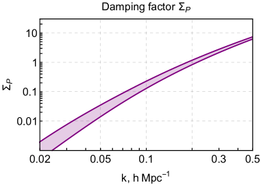
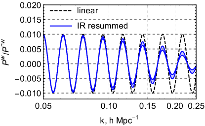
Figure 2: Damping of the primordial oscillations in the power spectrum by large bulk flows at redshift $z=0$. Left: the damping exponent. Right: Comparison of the wiggly power spectrum before and after IR resummation. We use the value $\gamma=30$. The bands show the change of the result when the separation scale $k_{S}$ is varied in the range $(0.3\div 0.7)k$.

Adding up the contributions (6.13) with all $\ell$ we obtain the leading-order IR-resummed wiggly power spectrum in a closed form,

$$P^{{\rm w,\,LO}}_{\delta\delta}(\eta;k)=g^{2}(\eta)e^{-g^{2}(\eta){\cal S}}P^{\rm w}_{L}(k)\,,$$ (6.15)

where we have introduced a new operator,

$${\cal S}=-\frac{1}{2}\int_{q\leq k_{S}}[dq]P_{L}^{\rm nw}(q)\mathcal{D}_{\bf q}\mathcal{D}_{-{\bf q}}\,.$$ (6.16)

The evaluation of its action at leading order in $\gamma$ and $\varepsilon$ gives (see Appendix C for details),

$${\cal S}P^{\rm w}_{L}(k)=\Sigma_{P}(k;k_{S})P^{\rm w}_{L}(k)\;,$$

$$\Sigma_{P}(k;k_{S})=\frac{k^{2}}{6\pi^{2}}\int_{0}^{k_{S}}\!\!dq\,P_{L}^{\rm nw}(q)\left[1-j_{0}\left(\frac{\gamma q}{k}\right)+2j_{2}\left(\frac{\gamma q}{k}\right)\right],$$ (6.17)

where $j_{0}$, $j_{2}$ are the spherical Bessel functions. Substituting this into (6.15) we see that the wiggly power spectrum is damped. The situation is very similar to the case of BAO [36, 55], with the only difference that the dependence of the damping factor $\Sigma_{P}$ on $k$ is now more complicated than quadratic. We show this dependence in the left panel of Fig. 2; the right panel illustrates the suppression of the wiggly power spectrum.

The total IR-resummed power spectrum at the leading order is obtained by adding the non-wiggly contribution that remains unmodified,

$$P_{\delta\delta}^{\rm LO}(\eta;k)=g^{2}(\eta)\Big{(}P_{L}^{\rm nw}(k)+e^{-g^{2}(\eta)\Sigma_{P}(k)}P_{L}^{\rm w}(k)\Big{)}\;.$$ (6.18)

The resummation procedure can be extended to include the corrections from the hard loops. We do not repeat the derivation here referring the interested reader to [36]. At the next-to-leading order in the hard loops the result reads,

$$P_{\delta\delta}^{\rm NLO}=g^{2}\Big{(}P_{L}^{\rm nw}+\big{(}1+g^{2}\Sigma_{P}\big{)}e^{-g^{2}\Sigma_{P}}P_{L}^{\rm w}\Big{)}+P_{\delta\delta}^{\text{1-loop}}\Big{[}P_{L}^{\rm nw}+e^{-g^{2}\Sigma_{P}}P_{L}^{\rm w}\Big{]}\;,$$ (6.19)

where the last term is the usual one-loop correction to the power spectrum evaluated using the linear spectrum with damped oscillations. Note that an extra contribution $g^{2}e^{-g^{2}\Sigma_{P}}P_{L}^{\rm w}$ in the first brackets is precisely what is needed to avoid double counting the soft part of the one-loop daisy diagram.

6.2 Bispectrum

We now include into consideration primordial non-Gaussianity. We will assume that it is purely oscillatory, as in our working example of the axion monodromy inflation (6.1b). In a more general case the derivation below would apply to the wiggly part of the bispectrum. For clarity, we will omit the oscillations in the primordial power spectrum (6.1a), whose effect was studied in the previous subsection, and focus on the oscillations in the bispectrum only.

6.2.1 Generic momenta

We first consider the case when all three momenta in the bispectrum are of the same order; the squeezed case with one soft momentum will be studied afterwards. We start by writing the IR enhanced terms in the quartic non-Gaussian vertex with three hard and one soft momentum. Using the relations (4.4) and the form of the $I_{2}$ kernel (A.1a) we obtain,

$$\begin{split}&\bar{\Gamma}_{4}^{\prime NG}({\bf k}_{1},{\bf k}_{2},-{\bf k}_{12}-{\bf q},{\bf q})\simeq\frac{1}{P_{L}(k_{1})P_{L}(k_{2})P_{L}(k_{12})}\\ &\quad\times\bigg{[}\frac{({\bf q}\cdot{\bf k}_{1})}{q^{2}}\big{(}B_{L}({\bf k}_{1}+{\bf q},{\bf k}_{2})-B_{L}({\bf k}_{1},{\bf k}_{2})\big{)}+\frac{({\bf q}\cdot{\bf k}_{2})}{q^{2}}\big{(}B_{L}({\bf k}_{1},{\bf k}_{2}+{\bf q})-B_{L}({\bf k}_{1},{\bf k}_{2})\big{)}\bigg{]},\end{split}$$ (6.20)

where we temporarily adopted the representation of the linear bispectrum as a function of two wavevectors (more precisely, of their lengths and the relative angle). Though not symmetric with respect to permutations in the three-point correlator, this representation turns out to be convenient for the derivation of the resummation formula. Equation (6.20) suggests to extend the action of operator $\mathcal{D}_{\bf q}$ introduced in Sec. 6.1 to the linear bispectrum,

$$\mathcal{D}_{\bf q}B_{L}({\bf k}_{1},{\bf k}_{2})=\bigg{[}\frac{({\bf q}\cdot{\bf k}_{1})}{q^{2}}\big{(}e^{{\bf q}\cdot\nabla_{{\bf k}^{\prime}_{1}}}-1\big{)}+\frac{({\bf q}\cdot{\bf k}_{2})}{q^{2}}\big{(}e^{{\bf q}\cdot\nabla_{{\bf k}^{\prime}_{2}}}-1\big{)}\bigg{]}B_{L}({\bf k}_{1}^{\prime},{\bf k}_{2}^{\prime})\Big{|}_{{\bf k}_{1}^{\prime}={\bf k}_{1},{\bf k}_{2}^{\prime}={\bf k}_{2}}.$$ (6.21)

Clearly, this operator is of order $1/\varepsilon$ in the IR power counting. By induction one can prove an analog of Eq. (6.8) for the leading IR-enhanced part of the non-Gaussian vertices (see Appendix C),

$$\bar{\Gamma}^{\prime NG}_{n}({\bf k}_{1},{\bf k}_{2},-{\bf k}_{12}-{\bf q}_{1\ldots(n-3)},{\bf q}_{1},...,{\bf q}_{n-3})\simeq\frac{(-1)^{n-2}}{P_{L}(k_{1})P_{L}(k_{2})P_{L}(k_{12})}\prod_{j=1}^{n-3}\mathcal{D}_{{\bf q}_{j}}B_{L}({\bf k}_{1},{\bf k}_{2})\,.$$ (6.22)

With this result at hand, it is straightforward to identify and resum the leading IR corrections to the non-Gaussian part of the bispectrum. Repeating the reasoning of Sec. 6.1 we obtain,

$$B^{NG,\,{\rm LO}}_{\delta\delta\delta}(\eta;{\bf k}_{1},{\bf k}_{2})=\fmffile{bstree}\begin{gathered}\fmfgraph*(60,60)\fmfpen{thick}\fmfleft{l1,l2,l3}\fmfright{r1,r2,r3}\fmf{plain,label=$ $}{l2,v2}\fmf{plain,label=$ $}{v2,r2}\fmf{phantom,label=$ $}{l1,v1}\fmf{phantom,label=$ $}{v1,r1}\fmf{plain,tension=0,label=$ $}{v2,v1}\fmfv{decor.shape=pentagram,decor.filled=empty,decor.size=7thick,label=$ $,l.a=120,l.d=.07w}{v2}\end{gathered}~{}+~{}\fmffile{softbs5}\begin{gathered}\fmfgraph*(60,60)\fmfpen{thick}\fmfkeep{1loop}\fmfleft{l1,l2,l3}\fmfright{r1,r2,r3}\fmfv{decor.shape=pentagram,decor.filled=empty,decor.size=7thick,label=$ $,l.a=120,l.d=.07w}{b1}\fmf{plain,label=$$}{b1,l2}\fmf{plain,label=$ $}{b1,r2}\fmf{phantom}{l1,u1}\fmf{phantom}{u2,r1}\fmf{phantom}{l3,v1}\fmf{phantom}{v2,r3}\fmf{phantom,right=0.5,tension=0.01,l.side=left}{b1,u1}\fmf{phantom,right=0.5,tension=2,label=$ $}{u1,u2}\fmf{phantom,left=0.5,tension=0.01}{b1,u2}\fmf{plain,left=0.5,tension=0.01,l.side=right}{b1,v1}\fmf{plain,left=0.5,tension=2,label=$ $}{v1,v2}\fmf{plain,right=0.5,tension=0.01}{b1,v2}\fmf{phantom,label=$ $}{l1,v3}\fmf{phantom,label=$ $}{v3,r1}\fmf{plain,tension=0,label=$ $}{v3,b1}\end{gathered}~{}+~{}\fmffile{softbs7}\begin{gathered}\fmfgraph*(60,60)\fmfpen{thick}\fmfleft{l0,l1,l12,l2,l223,l23,l3}\fmfright{r0,r1,r12,r2,l223,r23,r3}\fmfv{decor.shape=pentagram,decor.filled=empty,decor.size=7thick,label=$ $,l.a=120,l.d=.07w}{b1}\fmf{plain,label=$ $}{b1,l2}\fmf{plain,label=$ $}{b1,r2}\fmf{phantom,tension=0.04}{l1,u1}\fmf{phantom,tension=1}{u2,r1}\fmf{phantom,tension=1}{w2,r12}\fmf{phantom}{l3,v1}\fmf{phantom}{v2,r3}\fmf{plain,right=0.3,tension=0,l.side=left}{b1,u1}\fmf{plain,right=0.35,tension=0.1,label=$ $}{u1,u2}\fmf{plain,right=0.35,tension=0.1,label=$ $}{u2,w2}\fmf{plain,left=0.3,tension=0.1}{b1,w2}\fmf{plain,left=0.5,tension=0.01,l.side=right}{b1,v1}\fmf{plain,left=0.5,tension=2,label=$ $}{v1,v2}\fmf{plain,right=0.5,tension=0.01}{b1,v2}\fmf{phantom,label=$ $}{l0,v0}\fmf{phantom,label=$ $}{v0,r0}\fmf{plain,tension=0,label=$ $}{v0,b1}\end{gathered}~{}+~{}\ldots\;.$$ (6.26)

Evaluating the diagrams and summing them up we arrive at,

$$B^{NG,\,{\rm LO}}_{\delta\delta\delta}(\eta;{\bf k}_{1},{\bf k}_{2})=g^{3}(\eta)e^{-g^{2}(\eta){\cal S}}B_{L}({\bf k}_{1},{\bf k}_{2})\;,$$ (6.27)

where the operator ${\cal S}$ is still given by Eq. (6.16), with $\mathcal{D}_{\bf q}$ acting on the bispectrum as in (6.21). Note that until now we have not used any specific expression of the linear bispectrum, so the result of IR resummation in the operator form (6.27) is valid for any oscillating non-Gaussianity.

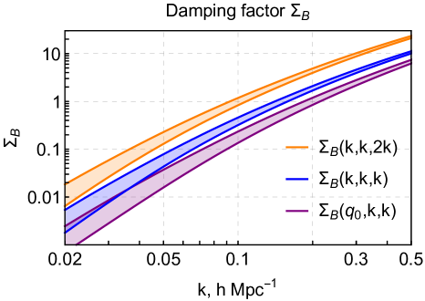
Figure 3: The damping factor of the resonant bispectrum for flattened, equilateral and squeezed shapes at redshift $z=0$. We use the value $\gamma=30$. The soft momentum in the squeezed case is $q_{0}=0.005\,h/\text{Mpc}$. The bands show the sensitivity of the result to the choice of the separation scale in the range $0.15k_{t}\leq k_{S}\leq 0.35k_{t}$.

Evaluation of the action of ${\cal S}$ leads to the damping of the oscillations in the bispectrum,

$$B^{NG,\,{\rm LO}}_{\delta\delta\delta}(\eta;k_{1},k_{2},k_{3})=g^{3}(\eta)e^{-g^{2}(\eta)\Sigma_{B}(k_{1},k_{2},k_{3})}B_{L}(k_{1},k_{2},k_{3})\;,$$ (6.28)

where we have switched back to the symmetric representation of $B$ as the function of three wavenumbers. The concrete expression for the damping factor depends on the model. In Appendix C we perform the calculation for the case of the resonant bispectrum (6.1b) with the result,

$$\begin{split}&\Sigma_{B}(k_{1},k_{2},k_{3})=\sum_{i<j}^{3}k_{i}k_{j}J\big{(}\hat{\bf k}_{i}\cdot\hat{\bf k}_{j}\big{)}\;,\\ &J(x)=\int_{q\leq k_{S}}\frac{dq}{6\pi^{2}}P_{L}(q)\left[-x+xj_{0}\left(\frac{\gamma q}{k_{t}}\sqrt{2(1-x)}\right)+\frac{3-x}{2}j_{2}\left(\frac{\gamma q}{k_{t}}\sqrt{2(1-x)}\right)\right]\,.\end{split}$$ (6.29)

Here $\hat{\bf k}_{i}$ is a unit vector directed along the momentum ${\bf k}_{i}$. One observes that, apart from the dependence on the absolute values of the momenta, the damping has a non-trivial dependence on the shape of the momentum triangle. This is illustrated in Fig. 3 where we show the dependence of $\Sigma_{B}$ on the momentum for several shapes. The IR separation scale is varied in the range $0.15k_{t}\leq k_{S}\leq 0.35k_{t}$. Note that with this choice $\Sigma_{B}$ reduces to the power spectrum damping $\Sigma_{P}(k_{1})$ in the squeezed limit $k_{3}\ll k_{1}\sim k_{2}$ (more on the squeezed limit below). We see that the dependence on $k_{S}$ is rather mild. As noted before, it provides an estimate of the uncertainty due to the neglect of the higher loop corrections. To illustrate the effect of damping, we split the bispectrum into the envelope $B_{\rm env}$ and oscillatory part $b_{\rm osc}$,

$$B_{L}=B_{\rm env}\cdot b_{\rm osc}\;,\qquad B_{\rm env}(k_{1},k_{2},k_{3})=4f_{NL}^{\rm res}{\cal A}_{\zeta}\,\sqrt{\frac{P_{L}(k_{1})P_{L}(k_{2})P_{L}(k_{3})}{k_{1}k_{2}k_{3}}}\;.$$ (6.30)

In Fig. 4 we show the effect of IR resummation on $b_{\rm osc}$ for the value of the frequency parameter $\gamma=30$. We observe that the oscillations are significantly damped at $k\gtrsim 0.07\,h/\text{Mpc}$ and get essentially washed out at $k\gtrsim 0.15\,h/\text{Mpc}$.

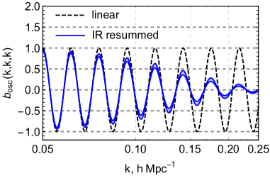
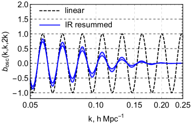
Figure 4: The oscillatory bispectrum before and after IR resummation for equilateral (left) and flattened (right) shapes. We take $\gamma=30$, $k_{*}=0.05\,h/\text{Mpc}$. The bands correspond to the variation of $k_{S}$ in the range $(0.15\div 0.35)k_{t}$. The redshift $z=0$.

6.2.2 The squeezed limit

So far we have been assuming that all three arguments of the bispectrum are of the same order, $k_{1}\sim k_{2}\sim k_{3}$. This assumption does not cover the squeezed limit when one of the momenta is soft. The latter limit is relevant for the scale-dependent halo bias. Besides, in the cosmological collider models of [19, 20, 21] this is precisely the limit that encodes the information about the masses and spins of heavy particles. Thus, it deserves a separate attention. We are going to see that it leads to new IR-enhanced contributions.

Consider again the non-Gaussian four-point vertex where now only two momenta are hard. A brief calculation gives its leading IR-enhanced part,

$$\bar{\Gamma}_{4}^{\prime NG}({\bf k},-{\bf k}-{\bf q}_{12},{\bf q}_{1},{\bf q}_{2})\simeq\frac{1}{\big{(}P_{L}(k)\big{)}^{2}}\bigg{[}\frac{1}{P_{L}(q_{2})}\mathcal{D}_{{\bf q}_{1}}B_{L}({\bf k},{\bf q}_{2})+\frac{1}{P_{L}(q_{1})}\mathcal{D}_{{\bf q}_{2}}B_{L}({\bf k},{\bf q}_{1})\bigg{]},$$ (6.31)

where the operator $\mathcal{D}_{\bf q}$ acts only on the hard momentum in the linear bispectrum,

$$\mathcal{D}_{\bf q}B_{L}({\bf k},{\bf q}^{\prime})=\frac{({\bf q}\cdot{\bf k})}{q^{2}}\big{(}e^{{\bf q}\nabla_{{\bf k}^{\prime}}}-1\big{)}B_{L}({\bf k}^{\prime},{\bf q}^{\prime})\Big{|}_{{\bf k}^{\prime}={\bf k}}\;.$$ (6.32)

In Appendix C we generalize this formula to an arbitrary $n$-point vertex,

$$\bar{\Gamma}^{\prime NG}_{n}({\bf k},-{\bf k}-{\bf q}_{1\ldots(n-2)},{\bf q}_{1},...,{\bf q}_{n-2})\simeq\frac{(-1)^{n-2}}{\big{(}P_{L}(k)\big{)}^{2}}\sum_{i=1}^{n-2}\frac{1}{P_{L}(q_{i})}\bigg{(}\prod_{j\neq i}^{n-3}\mathcal{D}_{{\bf q}_{j}}\bigg{)}B_{L}({\bf k},{\bf q}_{i})\,.$$ (6.33)

We observe that the leading IR term is of order $1/\varepsilon^{n-3}$, as in (6.22), but its structure is different. Therefore, the leading contributions to the squeezed bispectrum are still given by the diagrams (6.26), which, however, need to be re-evaluated. Denoting the soft external momentum by ${\bf q}_{0}$ we obtain for the $\ell$-loop term in the series,

$$\begin{split}&B_{\delta\delta\delta}^{NG,\,{\rm LO},\,\ell\text{-loop}}({\bf k},{\bf q}_{0})\simeq\;\frac{g^{3}}{\ell!}\bigg{(}\frac{g^{2}}{2}\bigg{)}^{\ell}\bigg{(}\int_{q\leq k_{S}}[dq]P_{L}(q)\mathcal{D}_{\bf q}\mathcal{D}_{-{\bf q}}\bigg{)}^{\ell}B_{L}({\bf k},{\bf q}_{0})\\ &\qquad\qquad\quad+\frac{g^{5}P_{L}(q_{0})}{(\ell-1)!}\bigg{(}\frac{g^{2}}{2}\bigg{)}^{\ell-1}\!\bigg{(}\!\int_{q\leq k_{S}}\!\![dq]P_{L}(q)\mathcal{D}_{\bf q}\mathcal{D}_{-{\bf q}}\!\bigg{)}^{\ell-1}\!\!\int_{q^{\prime}\leq k_{S}}\!\![dq^{\prime}]\mathcal{D}_{{\bf q}_{0}}\mathcal{D}_{-{\bf q}^{\prime}}B_{L}({\bf k},{\bf q}^{\prime})\;.\end{split}$$ (6.34)

Summation over $\ell$ yields the leading order squeezed bispectrum in the operator form,

$$B_{\delta\delta\delta}^{NG,\,{\rm LO}}(\eta;{\bf k},{\bf q}_{0})\!=\!g^{3}(\eta)e^{-g^{2}(\eta){\cal S}}B_{L}({\bf k},{\bf q}_{0})+g^{5}(\eta)P_{L}(q_{0})\!\!\int_{q\leq k_{S}}\!\!\![dq]\mathcal{D}_{{\bf q}_{0}}\mathcal{D}_{-{\bf q}}e^{-g^{2}(\eta){\cal S}}B_{L}({\bf k},{\bf q})\,.$$ (6.35)

The first term here is the same as Eq. (6.28). To see this we evaluate the action of the operator ${\cal S}$,

$${\cal S}B_{L}({\bf k},{\bf q}_{0})=\Sigma_{P}(k)B_{L}({\bf k},{\bf q}_{0})\;,$$ (6.36)

where $\Sigma_{P}$ is the power-spectrum damping factor (6.17). As discussed before, the latter coincides with the squeezed limit of the bispectrum damping $\Sigma_{B}$.

The second contribution in (6.35) is new. It describes the distortion of the oscillatory pattern produced by the long mode ${\bf q}_{0}$. Of course, this effect is non-vanishing only if $q_{0}\gtrsim k/\gamma$. In real space this corresponds to the requirement that the length of the long mode should be still shorter than the correlation length $l_{\rm corr}\sim\gamma/k$ set up by the momentum-space oscillations. Spelling out the operators in (6.35) we obtain an explicit expression,

$$B_{\delta\delta\delta}^{NG,\,{\rm LO}}(\eta;|{\bf k}-\tfrac{{\bf q}_{0}}{2}|,q_{0},|{\bf k}+\tfrac{{\bf q}_{0}}{2}|)=B_{(1)}(\eta;{\bf k},{\bf q}_{0})+B_{(2)}(\eta;{\bf k},{\bf q}_{0})\;,$$ (6.37)

where

$$B_{(1)}= g^{3}(\eta)e^{-g^{2}(\eta)\Sigma_{P}(k)}B_{L}(|{\bf k}-\tfrac{{\bf q}_{0}}{2}|,q_{0},|{\bf k}+\tfrac{{\bf q}_{0}}{2}|)\;,$$ (6.38a)

$$B_{(2)}= 2g^{5}(\eta)e^{-g^{2}(\eta)\Sigma_{P}(k)}P_{L}(q_{0})\frac{({\bf k}\cdot{\bf q}_{0})}{q_{0}^{2}}$$

$$\times\int_{q\leq k_{S}}[dq]\frac{({\bf k}\cdot{\bf q})}{q^{2}}\Big{(}B_{L}(|{\bf k}+\tfrac{{\bf q}_{0}}{2}|,q,|{\bf k}+\tfrac{{\bf q}_{0}}{2}+{\bf q}|)-B_{L}(|{\bf k}-\tfrac{{\bf q}_{0}}{2}|,q,|{\bf k}-\tfrac{{\bf q}_{0}}{2}+{\bf q}|)\Big{)}.$$ (6.38b)

Note that we have shifted the hard momentum ${\bf k}\mapsto{\bf k}-\frac{{\bf q}_{0}}{2}$ to somewhat simplify the subsequent formulas.

Evaluation of the resonant bispectrum in the squeezed limit is subtle. Taken at face value, the expression (6.1b) will be dominated at $q\lesssim k/\gamma$ by the second term in the square brackets. The latter can be written as

$$B_{\zeta}\Big{|}_{q\to 0,\;k_{1}=|{\bf k}-\tfrac{{\bf q}}{2}|}\simeq f_{NL}^{\rm res}\frac{4{\cal A}_{\zeta}^{4}}{k^{4}q^{2}}\cdot\frac{2k}{\gamma q}\cos\Big{(}\gamma\mathop{\rm ln}\nolimits\frac{2k}{k_{*}}\Big{)}=-P_{\zeta}(q)P_{\zeta}(k)\frac{d\mathop{\rm ln}\nolimits(k^{3}P_{\zeta}(k))}{d\mathop{\rm ln}\nolimits k}\;,$$ (6.39)

which is precisely of the form dictated by the Maldacena consistency condition [56]. It is known that such terms drop from physical observables. In particular, they cancel out if one transforms the bispectrum from the comoving coordinates used to derive (6.1b) to conformal Fermi coordinates (CFC) [57]. In the latter frame the leading contribution into squeezed primordial bispectrum of a single-field slow-roll inflation scales as $O(q^{2}/k^{2})$. Thus, to avoid unphysical contributions, the term (6.39) must be subtracted. On the other hand, the construction of the CFC frame is possible only if the wavelength of the long mode is larger than all other relevant scales. It breaks down when the length of the long mode becomes comparable to the correlation length $l_{\rm corr}\sim\gamma/k$. In other words, while we can easily obtain an unambiguous physical squeezed limit of the bispectrum at $q\ll k/\gamma$ using CFC, it is no longer possible at $k/\gamma\lesssim q\ll k$. A proper definition of the physical bispectrum in the intermediate range presents an open issue and may require taking into account the projection effects pertaining to the actual physical quantities measured by an observer on Earth. Such study is beyond the scope of this paper. Instead, we adopt a simplified approach and model the expected form of the physical bispectrum by subtracting from (6.1b) the term (6.39) weighted with a function $w\big{(}\frac{\gamma q}{2k}\big{)}$ that interpolates between $w=1+O(x^{2})$ at $x\to 0$ and $w=0$ at $x\to\infty$; in the practical calculations we will use $w=(1+x^{2})^{-1}$. This model cannot be judged fully satisfactory. In particular, it likely introduces an order-one error compared to the true bispectrum at $\frac{\gamma q}{2k}\sim 1$. Nevertheless, it is sufficient for our purposes of illustrating the dynamical effects of large bulk flows.

With the above caveat in mind, we will use the following form of the squeezed linear bispectrum,

$$\begin{split}B_{L}(|{\bf k}-\tfrac{{\bf q}}{2}|,q,|{\bf k}+\tfrac{{\bf q}}{2}|)=&B_{\rm env}(k,k,q)\bigg{[}\sin\Big{(}\gamma\mathop{\rm ln}\nolimits\frac{2k}{k_{*}}\Big{)}\bigg{(}\cos\Big{(}\frac{\gamma q}{2k}\Big{)}-\frac{2k}{\gamma q}\sin\Big{(}\frac{\gamma q}{2k}\Big{)}\bigg{)}\\ &+\cos\Big{(}\gamma\mathop{\rm ln}\nolimits\frac{2k}{k_{*}}\Big{)}\bigg{(}\sin\Big{(}\frac{\gamma q}{2k}\Big{)}+\frac{2k}{\gamma q}\bigg{(}\cos\Big{(}\frac{\gamma q}{2k}\Big{)}-w\Big{(}\frac{\gamma q}{2k}\Big{)}\bigg{)}\bigg{)}\bigg{]},\end{split}$$ (6.40)

where the smooth enveloping function $B_{\rm env}$ is defined in (6.30). This form directly determines the contribution $B_{(1)}$ of the IR resummed bispectrum, which differs from the linear bispectrum only by the damping of oscillations. To find the second contribution $B_{(2)}$ one substitutes (6.40) into (6.38b). Integration over the directions of $q$ yields,

$$\begin{split}\frac{B_{(2)}(\eta;{\bf k},{\bf q}_{0})}{B_{\rm env}(k,k,q_{0})}=&4g^{5}(\eta)e^{-g^{2}(\eta)\Sigma_{P}(k)}\,k\sqrt{q_{0}P_{L}(q_{0})}\,\frac{({\bf k}\cdot{\bf q}_{0})}{q_{0}^{2}}\sin\bigg{(}\gamma\frac{({\bf k}\cdot{\bf q}_{0})}{2k^{2}}\bigg{)}\\ &\times\bigg{[}C_{1}(k;k_{S})\sin\Big{(}\gamma\mathop{\rm ln}\nolimits\frac{2k}{k_{*}}\Big{)}+C_{2}(k;k_{S})\cos\Big{(}\gamma\mathop{\rm ln}\nolimits\frac{2k}{k_{*}}\Big{)}\bigg{]},\end{split}$$ (6.41)

with

$$C_{1}= \int_{q\leq k_{S}}\frac{dq}{2\pi^{2}}\sqrt{qP_{L}(q)}\;j_{1}\Big{(}\frac{\gamma q}{2k}\Big{)}\bigg{[}\frac{2k}{\gamma q}\sin\Big{(}\frac{\gamma q}{2k}\Big{)}-\cos\Big{(}\frac{\gamma q}{2k}\Big{)}\bigg{]},$$ (6.42a)

$$C_{2}= -\int_{q\leq k_{S}}\frac{dq}{2\pi^{2}}\sqrt{qP_{L}(q)}\;j_{1}\Big{(}\frac{\gamma q}{2k}\Big{)}\bigg{[}\sin\Big{(}\frac{\gamma q}{2k}\Big{)}+\frac{2k}{\gamma q}\bigg{(}\cos\Big{(}\frac{\gamma q}{2k}\Big{)}-w\Big{(}\frac{\gamma q}{2k}\Big{)}\bigg{)}\bigg{]}.$$ (6.42b)

Note the peculiar dependence of the expression (6.41) on the angle between the soft and hard momenta: for $q_{0}\gg k/\gamma$ it rapidly oscillates as a function of the angle, whereas at $q_{0}\ll k/\gamma$ it reduces to the sum of monopole and quadrupole. We plot the contributions $B_{(1)}$, $B_{(2)}$ (for collinear ${\bf k}$ and ${\bf q}_{0}$) as functions of the hard momentum $k$ in Fig. 5. We observe the damping of oscillations in $B_{(1)}$ above $k\sim 0.15h/\text{Mpc}$, though the effect is somewhat weaker than in the equilateral and flattened cases. The behavior of $B_{(2)}$ is quite different: its amplitude grows from small $k$ up to $k\sim 0.2h/\text{Mpc}$ and only then starts decaying exponentially. In Fig. 6 we plot the components of the squeezed bispectrum as functions of the soft momentum at fixed $k$.

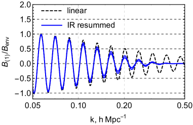
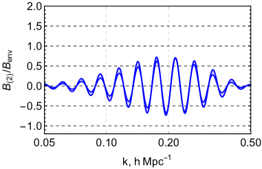
Figure 5: The components $B_{(1)}$ (left) and $B_{(2)}$ (right) of IR resummed squeezed bispectrum as functions of the hard momentum for the value of the soft momentum $q_{0}=0.005\,h/\text{Mpc}$. The hard and soft momenta are taken to be collinear; $\gamma=30$, $k_{*}=0.05\,h/\text{Mpc}$ . The bands correspond to the variation of $k_{S}$ in the range $(0.3\div 0.7)k$. The redshift $z=0$.

Finally, let us notice that the squeezed limit of the resonant bispectrum, through the mode coupling, produces an additional oscillating contribution in the power spectrum on top of the primordial one (6.4). Its leading part can be found using again the method of IR resummation. It is given by the sum of daisy diagrams,

$$\Delta P^{\rm w,\,LO}_{\delta\delta}(k)=\fmffile{wiggly4bs}\begin{gathered}\fmfgraph*(60,60)\fmfpen{thick}\fmfkeep{1loop}\fmfleft{l1,l2,l3}\fmfright{r1,r2,r3}\fmfv{decor.shape=pentagram,decor.filled=empty,decor.size=7thick,label=$ $,l.a=120,l.d=.07w}{b1}\fmf{plain,label=$$}{b1,l2}\fmf{plain,label=$ $}{b1,r2}\fmf{phantom}{l1,u1}\fmf{phantom}{u2,r1}\fmf{phantom}{l3,v1}\fmf{phantom}{v2,r3}\fmf{phantom,right=0.5,tension=0.01,l.side=left}{b1,u1}\fmf{phantom,right=0.5,tension=2,label=$ $}{u1,u2}\fmf{phantom,left=0.5,tension=0.01}{b1,u2}\fmf{plain,left=0.5,tension=0.01,l.side=right}{b1,v1}\fmf{plain,left=0.5,tension=2,label=$ $}{v1,v2}\fmf{plain,right=0.5,tension=0.01}{b1,v2}\end{gathered}~{}+~{}\fmffile{wiggly6bs}\begin{gathered}\fmfgraph*(60,60)\fmfpen{thick}\fmfkeep{2loop}\fmfleft{l1,l2,l3}\fmfright{r1,r2,r3}\fmfv{decor.shape=pentagram,decor.filled=empty,decor.size=7thick,label=$ $,l.a=120,l.d=.07w}{b1}\fmf{plain,label=$ $}{b1,l2}\fmf{plain,label=$ $}{b1,r2}\fmf{phantom}{l1,u1}\fmf{phantom}{u2,r1}\fmf{phantom}{l3,v1}\fmf{phantom}{v2,r3}\fmf{plain,right=0.5,tension=0.01,l.side=left}{b1,u1}\fmf{plain,right=0.5,tension=2,label=$ $}{u1,u2}\fmf{plain,left=0.5,tension=0.01}{b1,u2}\fmf{plain,left=0.5,tension=0.01,l.side=right}{b1,v1}\fmf{plain,left=0.5,tension=2,label=$ $}{v1,v2}\fmf{plain,right=0.5,tension=0.01}{b1,v2}\end{gathered}~{}+~{}\ldots=-g^{3}e^{-g^{2}{\cal S}}\int_{q\leq k_{S}}[dq]\mathcal{D}_{-{\bf q}}B_{L}({\bf k},{\bf q})\;,$$ (6.45)

where we made use of the expression (6.33) for the TSPT vertices to compute different terms in the series. The structure of this result is intuitively clear. Working out the action of the operators ${\cal S}$, $\mathcal{D}_{-{\bf q}}$ one recognizes in it the leading IR part of the usual one-loop correction to the power spectrum (last term in Eq. (2.19b)), with an extra exponential damping. Substituting the explicit form of the squeezed linear bispectrum (6.40) we obtain,

$$\Delta P^{\rm w,\,LO}_{\delta\delta}(\eta;k)=8f_{NL}^{\rm res}{\cal A}_{\zeta}g^{3}(\eta)e^{-g^{2}(\eta)\Sigma_{P}(k)}P_{L}(k)\bigg{[}C_{1}(k)\cos\Big{(}\!\gamma\mathop{\rm ln}\nolimits\frac{2k}{k_{*}}\Big{)}-C_{2}(k)\sin\Big{(}\!\gamma\mathop{\rm ln}\nolimits\frac{2k}{k_{*}}\Big{)}\bigg{]},$$ (6.46)

where the coefficients $C_{1}$, $C_{2}$ are given in (6.42). Given the measured value of ${\cal A}_{\zeta}$, this contribution is always small. Further, the relation (6.2) implies that it is subdominant compared to the primordial wiggly power spectrum as long as $\gamma<100$. Thus, in our working example of the primordial non-Gaussianity produced in the axion monodromy inflation this contribution appears uninteresting. However, it may be relevant in other models where the oscillating component in the primordial power spectrum is absent or strongly suppressed. This situation occurs, for example, in the context of cosmological colliders [19, 20, 21].

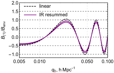
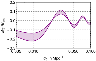
Figure 6: The components $B_{(1)}$ (left) and $B_{(2)}$ (right) of IR resummed squeezed bispectrum as functions of the soft momentum for the hard momentum $k=0.1\,h/\text{Mpc}$. The hard and soft momenta are taken to be collinear; $\gamma=30$, $k_{*}=0.05\,h/\text{Mpc}$ . The bands correspond to the variation of $k_{S}$ in the range $(0.3\div 0.7)k$. The redshift $z=0$.

7 Conclusion

In this paper we worked out the TSPT framework for non-Gaussian primordial statistics. They are included by setting appropriate initial conditions for the TSPT statistical weight, which eventually modifies only the vertices $\Gamma_{n}$. Other building blocks of TSPT, such as the composite operator kernels $K_{n}$ and counterterms $C_{n}$ remain intact. In this way TSPT can easily accommodate any sort of non-Gaussian initial conditions without a significant modification of the formalism. Treating initial non-Gaussian contributions as small deformations of the Gaussian statistical weight generates a new perturbative expansion on top of the usual TSPT perturbation series. We have shown that the new non-Gaussian TSPT vertices are manifestly IR safe, implying IR safety of the non-Gaussian TSPT Feynman diagrams.

TSPT with non-Gaussian initial conditions opens a new way to study the effects of primordial non-Gaussianity on LSS clustering. As an application, we developed a new procedure to capture the non-linear evolution of primordial oscillating features that may be imprinted in the power spectrum and higher statistics during inflation. We showed that such oscillations are suppressed by nonlinear effects of bulk motions, just like BAO. We demonstrated how to calculate the damping factor by resummation of IR enhanced diagrams and computed it explicitly for the resonant power spectrum and bispectrum from axion monodromy inflation. We point out that the damping of primordial oscillating features due to large bulk flows has been overlooked in many studies of future survey sensitivities. Taking it into account can significantly affect the forecasts. It will also be interesting to study to what extent the damping can be removed using the density field reconstruction technique [59, 60].

We have found that in the case of squeezed bispectrum the IR resummation, apart from damping, produces an additional contribution depending on the angle between the hard and soft momenta. It will be interesting to study observable signatures of this term, in particular, to what extent it can be discriminated from the primordial angular dependence of the squeezed bispectrum in the cosmological collider models.

The results of this work reinforce the status of IR resummation in TSPT as a universal systematic procedure, applicable beyond the case of Gaussian initial conditions. They can be extended in several directions. While in the current paper we focused on the power spectrum and bispectrum, the IR resummation can be straightforwardly applied to higher primordial statistics, in particular, to the trispectrum which may possess oscillating features due to an exchange of massive particles [19, 20, 21]. Next, it would be interesting to incorporate the effects of redshift space distortions in the IR-resummed non-Gaussian statistics; this can be done along the lines of [37]. One would also like to extend the non-Gaussian IR resummation beyond the leading order to include the contributions of loop diagrams with hard momenta and subleading IR corrections, as done for the Gaussian case in Ref. [36].

Last but not least, we adopted in this paper the pressureless perfect fluid approximation. To properly renormalize the contributions of short scales, the non-Gaussian TSPT should be embedded in the framework of EFT of LSS [8, 9, 10]. We leave this task for future.

Note added. When this paper was completed, we became aware of the work [61] that also discusses the damping of the primordial oscillation features in the power spectrum. When overlap, our results agree. We thank the authors of [61] for sharing with us the preliminary version of the paper.

Acknowledgments

We thank Diego Blas, Mathias Garny, Azadeh Moradinezhad Dizgah, Alvise Raccanelli, Marko Simonović, Fabian Schmidt, Zvonimir Vlah and Benjamin Wallisch for useful discussions. M.I. thanks the CERN Theory Department for hospitality during the completion of this work. M.I. acknowledges the support by the RFBR grant 17-02-01008. The work of S.S. is supported by the Swiss National Science Foundation and the RFBR grant 17-02-00651. The work of A.V. is supported by the Danish National Research Foundation (DNRF91). M.I. is partially supported by the Simons Foundation’s Origins of the Universe program.

Appendix A TSPT kernels

The basic building blocks of TSPT are the kernels $I_{n}$ and $K_{n}$ defined in Eqs. (3.1), (3.2). They satisfy a set of recursion relations [35] that are derived from the dynamical equations of motion (2.15). The seeds for these relations are $I_{1}=K_{1}=1$, as follows from the linear evolution, assuming adiabatic initial conditions. By substituting the representation (3.1) into the Euler equation (2.15b) and comparing with (3.2) we express the kernels $I_{n}$ in terms of $K_{n}$,

$$I_{2}({\bf k}_{1},{\bf k}_{2})=2\beta({\bf k}_{1},{\bf k}_{2})+\frac{3}{2}K_{2}({\bf k}_{1},{\bf k}_{2})\;,$$ (A.1a)

$$I_{n}({\bf k}_{1},\ldots,{\bf k}_{n})=\frac{3}{2}K_{n}({\bf k}_{1},\ldots,{\bf k}_{n})~{},~{}~{}~{}~{}n\geq 3\;.$$ (A.1b)

Next, the expressions (3.1), (3.2) are put into the continuity equation (2.15a). Comparing the terms of the same order in $\Theta({\bf k})$ and using the relations (A.1) we obtain the recursive formulas,

$$K_{2}({\bf k}_{1},{\bf k}_{2})=\frac{2}{7}\Big{(} \alpha({\bf k}_{1},{\bf k}_{2})+\alpha({\bf k}_{2},{\bf k}_{2})-2\beta({\bf k}_{1},{\bf k}_{2})\Big{)}=\frac{4}{7}\sin^{2}({\bf k}_{1},{\bf k}_{2})\;,$$ (A.2a)

$$K_{n}({\bf k}_{1},...,{\bf k}_{n})= \frac{2}{2n+3}\bigg{[}\sum_{i=1}^{n}\alpha\big{(}{\bf k}_{i},{\bf k}_{1\ldots n}-k_{i}\big{)}\,K_{n-1}\big{(}{\bf k}_{1},...,\check{{\bf k}}_{i},...,{\bf k}_{n}\big{)}$$

$$-2\sum_{i<j}\beta({\bf k}_{i},{\bf k}_{j})\,K_{n-1}\big{(}{\bf k}_{i}+{\bf k}_{j},{\bf k}_{1},...,\check{\bf k}_{i},...,\check{\bf k}_{j},...,{\bf k}_{n}\big{)}$$

$$-\frac{3}{2}\sum_{m=2}^{n-1}\sum_{\sigma}\frac{K_{m}\big{(}{\bf k}_{\sigma(1)},...,{\bf k}_{\sigma(m)}\big{)}}{m!(n-m)!}\,K_{n-m+1}\Big{(}\sum_{i=1}^{m}{\bf k}_{\sigma(i)},{\bf k}_{\sigma(m+1)},...,{\bf k}_{\sigma(n)}\Big{)}\Bigg{]}.$$ (A.2b)

The notation $\check{\bf k}_{i}$ above means that the momentum ${\bf k}_{i}$ is absent from the arguments of the corresponding function, and in the last line of (A.2b) the summation is performed over all permutations $\sigma$ of $n$ indices.

Appendix B One-loop non-Gaussian power spectrum

In this Appendix we illustrate the application of TSPT Feynman rules on the example of 1-loop corrections to the power spectrum involving primordial non-Gaussianity. The corresponding diagrams are shown in (4.7). To evaluate them, we need, in addition to the cubic non-Gaussian vertex (4.4a), also the expressions for the cubic Gaussian and quartic non-Gaussian vertices. These are easily obtained using the recursion relations (3.14b), (4.4b) and read,

$$\bar{\Gamma}_{3}({\bf k}_{1},{\bf k}_{2},{\bf k}_{3})=-(2\pi)^{3}\delta_{D}^{(3)}(k_{123})\bigg{[}\frac{I_{2}({\bf k}_{1},{\bf k}_{2})}{P_{L}(k_{3})}+\text{cyclic}\bigg{]}\;,$$ (B.1)

$$\bar{\Gamma}_{4}^{NG}({\bf k}_{1},{\bf k}_{2},{\bf k}_{3},{\bf k}_{4})=(2\pi)^{3}\delta^{(3)}_{D}({\bf k}_{1\ldots 4})\!\!\sum_{1\leq i<j\leq 4}\!\!I_{2}({{\bf k}_{i}},{{\bf k}_{j}})\frac{B_{L}\big{(}\lvert{\bf k}_{i}+{\bf k}_{j}\rvert,k_{l},k_{m}\big{)}}{P_{L}(\lvert{\bf k}_{i}+{\bf k}_{j}\rvert)P_{L}(k_{l})P_{L}(k_{m})}\bigg{|}_{\begin{smallmatrix}&l<m\\ &l,m\neq i,j\end{smallmatrix}}\;,$$ (B.2)

Now we are ready to write the expressions corresponding to the three diagrams in (4.7). For the first diagram, which we call ‘daisy’, we obtain,

$$\begin{split}P_{\Theta\Theta,\,{\rm daisy}}^{NG,\,\text{1-loop}}&=-\frac{1}{2}g^{3}(\eta)\big{(}P_{L}(k)\big{)}^{2}\int[dq]P_{L}(q){\bar{\Gamma}_{4}^{\prime NG}}({\bf q},-{\bf q},{\bf k},-{\bf k})\\ &=-2g^{3}(\eta)P_{L}(k)\int[dq]B_{L}(k,q,|{\bf k}+{\bf q}|)\frac{I_{2}({\bf k},{\bf q})}{P_{L}(|{\bf k}+{\bf q}|)}\,.\end{split}$$ (B.3)

The second diagram (‘fish’) gives,

$$\begin{split}P_{\Theta\Theta,\,{\rm fish}}^{NG,\,\text{1-loop}}&=g^{3}(\eta)\big{(}P_{L}(k)\big{)}^{2}\int[dq]\bar{\Gamma}_{3}^{\prime NG}({\bf k},{\bf q},-{\bf k}-{\bf q})\bar{\Gamma}_{3}^{\prime}({\bf k}+{\bf q},-{\bf q},-{\bf k})P_{L}(q)P_{L}(|{\bf k}+{\bf q}|)\\ &=g^{3}(\eta)\int[dq]B_{L}(k,q,|{\bf k}+{\bf q}|)\left[\frac{2I_{2}({\bf k},{\bf q})P_{L}(k)}{P_{L}(|{\bf k}+{\bf q}|)}+I_{2}({\bf k}+{\bf q},-{\bf q})\right].\end{split}$$ (B.4)

In deriving these expressions we used the following properties of the kernel $I_{2}$,

$$I_{2}({\bf k},-{\bf k})=0~{},~{}~{}~{}~{}~{}I_{2}(-{\bf k},-{\bf q})=I_{2}({\bf k},{\bf q})\;.$$

Finally, the last diagram (‘composite fish’) reads,

$$\begin{split}P_{\delta\delta,\,\text{comp.\,fish}}^{NG,\,\text{1-loop}}&=-g^{3}(\eta)P_{L}(k)\int[dq]K_{2}({\bf k}+{\bf q},-{\bf q})\bar{\Gamma}_{3}^{\prime NG}({\bf k}+{\bf q},-{\bf q},-{\bf k})P_{L}(q)P_{L}(|{\bf k}+{\bf q}|)\\ &=g^{3}(\eta)\int[dq]B_{L}(k,q,|{\bf k}+{\bf q}|)K_{2}({\bf k}+{\bf q},-{\bf q})\;.\end{split}$$ (B.5)

Collecting the three contributions together we arrive at

$$P_{\delta\delta}^{NG,\,\text{1-loop}}=g(\eta)^{3}\int[dq]B_{L}(k,q,\lvert{\bf k}+{\bf q}\rvert)\big{(}I_{2}({\bf k}+{\bf q},-{\bf q})+K_{2}({\bf k}+{\bf q},-{\bf q})\big{)}\;.$$ (B.6)

The kernels $I_{2}$, $K_{2}$ are to be taken from Eqs. (A.1a), (A.2a). Using the relation between the TSPT and SPT kernels established in [35], $I_{2}+K_{2}=2F_{2}$, one recognizes in (B.6) the standard SPT result, see Eq. (2.19b).

Appendix C Technical details of IR resummation

C.1 IR enhancement of the TSPT vertices

In this subsection we derive Eqs. (6.8), (6.22), (6.33). The derivation is done by induction. Let us start with the Gaussian vertices. Assume that Eq. (6.8) holds for all vertices with $n^{\prime}\leq n-1$ and consider the recursion relation (3.14b) for the $n$-th vertex:

$$\begin{split}\bar{\Gamma}^{\prime\rm w}_{n}({\bf k},-{\bf k}-&{\bf q}_{tot},{\bf q}_{1},...,{\bf q}_{n-2})=-\frac{1}{n-2}\bigg{[}I_{2}({\bf k},-{\bf k}-{\bf q}_{tot})\bar{\Gamma}_{n-1}^{\prime\rm w}({\bf q}_{tot},{\bf q}_{1},...,{\bf q}_{n-2})\\ &+\sum_{i=1}^{n-2}I_{2}({\bf k},{\bf q}_{i})\bar{\Gamma}^{\prime\rm w}_{n-1}({\bf k}+{\bf q}_{i},-{\bf k}-{\bf q}_{tot},{\bf q}_{1},...,\check{{\bf q}}_{i},...,{\bf q}_{n-2})\\ &+\sum_{i=1}^{n-2}I_{2}(-{\bf k}-{\bf q}_{tot},{\bf q}_{i})\bar{\Gamma}^{\prime\rm w}_{n-1}(-{\bf k}-{\bf q}_{tot}+{\bf q}_{i},{\bf k},{\bf q}_{1},...,\check{{\bf q}}_{i},...,{\bf q}_{n-2})\\ &+\sum_{i<j}^{n-2}I_{2}({\bf q}_{i},{\bf q}_{j})\bar{\Gamma}^{\prime\rm w}_{n-1}({\bf q}_{i}+{\bf q}_{j},{\bf k},-{\bf k}-{\bf q}_{tot},{\bf q}_{1},...,\check{{\bf q}}_{i},...,\check{{\bf q}}_{j}...,{\bf q}_{n-2})+\ldots\bigg{]},\end{split}$$ (C.1)

where we have denoted by ${\bf q}_{tot}$ the sum of all soft momenta. Dots in the last line stand for the terms involving the vertices $\bar{\Gamma}_{n^{\prime}}^{\prime\rm w}$ with $n^{\prime}\leq n-2$ and kernels $I_{m}$ with $m\geq 3$. All the latter kernels are IR safe, hence the omitted terms are at most of order $1/\varepsilon^{n-4}$. At the leading IR order they can be neglected. The kernel $I_{2}$ has a singularity only if one of its momenta is hard and the other is soft. Otherwise it is of order one. This implies that the terms in the first and last lines of (C.1) are at most of order $1/\varepsilon^{n-3}$ and can be neglected as well. One is left with the contributions of the second and third lines. The next step is to use the IR asymptotics

$$I_{2}({\bf k},{\bf q})\simeq\frac{({\bf q}\cdot{\bf k})}{q^{2}}$$ (C.2)

and the expression (6.8) for $\bar{\Gamma}_{n-1}^{\prime\rm w}$. This yields,

$$\begin{split}\bar{\Gamma}^{\prime\rm w}_{n}({\bf k},-{\bf k}-{\bf q}_{tot},{\bf q}_{1},...,{\bf q}_{n-2})\simeq\frac{(-1)^{n-1}}{(n-2)\big{(}P_{L}^{\rm nw}(k)\big{)}^{2}}\bigg{[}&\sum_{i=1}^{n-2}\frac{({\bf q}_{i}\cdot{\bf k})}{q_{i}^{2}}\prod_{j\neq i}^{n-2}\mathcal{D}_{{\bf q}_{j}}P_{L}^{\rm w}(|{\bf k}+{\bf q}_{i}|)\\ &-\sum_{i=1}^{n-2}\frac{({\bf q}_{i}\cdot{\bf k})}{q_{i}^{2}}\prod_{j\neq i}^{n-2}\mathcal{D}_{{\bf q}_{j}}P_{L}^{\rm w}({\bf k})\bigg{]}.\end{split}$$ (C.3)

The terms in the square brackets combine to produce the operator $\mathcal{D}_{{\bf q}_{i}}$. Using the commutativity of operators $\mathcal{D}_{\bf q}$ with different ${\bf q}$’s one arrives at Eq. (6.8). $\blacksquare$

We now turn to the proof of Eq. (6.22). We again assume that it holds for $n^{\prime}\leq n-1$ and consider the relation (4.4b) defining the $n$-th vertex. Keeping only the terms containing the IR-enhanced kernels $I_{2}$ we obtain,

$$\begin{split}&\bar{\Gamma}_{n}^{\prime NG}({\bf k}_{1},{\bf k}_{2},-{\bf k}_{12}-{\bf q}_{tot},{\bf q}_{1},...{\bf q}_{n-3})\\ &=-\frac{1}{n-3}\bigg{[}\sum_{i=1}^{n-3}I_{2}({\bf k}_{1},{\bf q}_{i})\bar{\Gamma}_{n-1}^{\prime NG}({\bf k}_{1}+{\bf q}_{i},{\bf k}_{2},-{\bf k}_{12}-{\bf q}_{tot},{\bf q}_{1},...\check{{\bf q}}_{i},...{\bf q}_{n-3})\\ &\quad+\sum_{i=1}^{n-3}I_{2}({\bf k}_{2},{\bf q}_{i})\bar{\Gamma}_{n-1}^{\prime NG}({\bf k}_{2}+{\bf q}_{i},{\bf k}_{1},-{\bf k}_{12}-{\bf q}_{tot},{\bf q}_{1},...\check{{\bf q}}_{i},...{\bf q}_{n-3})\\ &\quad+\sum_{i=1}^{n-3}I_{2}(-{\bf k}_{12}-{\bf q}_{tot},{\bf q}_{i})\bar{\Gamma}_{n-1}^{\prime NG}(-{\bf k}_{12}-{\bf q}_{tot}+{\bf q}_{i},{\bf k}_{1},{\bf k}_{2},{\bf q}_{1},...\check{{\bf q}}_{i},...{\bf q}_{n-3})+\ldots\bigg{]},\end{split}$$ (C.4)

where dots correspond to the terms that are at most of order $1/\varepsilon^{n-4}$. Using next Eq. (C.2) and substituting the leading IR part of $\bar{\Gamma}_{n-1}^{\prime NG}$ we get,

$$\begin{split}&\bar{\Gamma}_{n}^{\prime NG}({\bf k}_{1},{\bf k}_{2},-{\bf k}_{12}-{\bf q}_{tot},{\bf q}_{1},...{\bf q}_{n-3})\simeq\frac{(-1)^{n-2}}{(n-3)P_{L}(k_{1})P_{L}(k_{2})P_{L}(k_{12})}\\ &\times\!\sum_{i=1}^{n-3}\prod_{j\neq i}^{n-3}\mathcal{D}_{{\bf q}_{j}}\bigg{[}\frac{({\bf q}_{i}\cdot{\bf k}_{1})}{q_{i}^{2}}B_{L}({\bf k}_{1}\!+\!{\bf q}_{i},{\bf k}_{2})+\frac{({\bf q}_{i}\cdot{\bf k}_{2})}{q_{i}^{2}}B_{L}({\bf k}_{1},{\bf k}_{2}\!+\!{\bf q}_{i})-\frac{({\bf q}_{i}\cdot{\bf k}_{12})}{q_{i}^{2}}B_{L}({\bf k}_{1},{\bf k}_{2})\bigg{]}.\end{split}$$ (C.5)

Recalling that ${\bf k}_{12}={\bf k}_{1}+{\bf k}_{2}$ we recognize in the square brackets the operator $\mathcal{D}_{{\bf q}_{i}}$ which completes the product of operators to $\prod_{j=1}^{n-3}\mathcal{D}_{{\bf q}_{j}}$. Summation over $i$ then cancels the factor $(n-3)$ in the denominator and we obtain (6.22). $\blacksquare$

Finally, we give the proof of Eq. (6.33). The strategy is the same as in the two previous cases: we assume that it is valid for $n^{\prime}\leq n-1$ and study the vertex $\Gamma_{n}^{\prime NG}$. The leading contribution containing the IR-enhanced $I_{2}$ kernels is

$$\begin{split}\bar{\Gamma}_{n}^{\prime NG}({\bf k},&-{\bf k}-{\bf q}_{tot},{\bf q}_{1},...{\bf q}_{n-2})\\ =&-\frac{1}{n-3}\bigg{[}\sum_{i=1}^{n-2}I_{2}({\bf k},{\bf q}_{i})\bar{\Gamma}_{n-1}^{\prime NG}({\bf k}+{\bf q}_{i},-{\bf k}-{\bf q}_{tot},{\bf q}_{1},...\check{{\bf q}}_{i},...{\bf q}_{n-2})\\ &+\sum_{i=1}^{n-2}I_{2}(-{\bf k}-{\bf q}_{tot},{\bf q}_{i})\bar{\Gamma}_{n-1}^{\prime NG}(-{\bf k}-{\bf q}_{tot}+{\bf q}_{i},{\bf k},{\bf q}_{1},...\check{{\bf q}}_{i},...{\bf q}_{n-2})+\ldots\bigg{]}.\end{split}$$ (C.6)

Substituting the IR asymptotics of $I_{2}$ and $\bar{\Gamma}_{n-1}^{\prime NG}$ we obtain,

$$\begin{split}\bar{\Gamma}_{n}^{\prime NG}({\bf k},-{\bf k}-{\bf q}_{tot},{\bf q}_{1},...{\bf q}_{n-2})\simeq\frac{(-1)^{n-2}}{(n-3)\big{(}P_{L}(k)\big{)}^{2}}\sum_{i=1}^{n-2}\sum_{j\neq i}^{n-2}\frac{1}{P_{L}(q_{j})}\prod_{l\neq j}^{n-2}\mathcal{D}_{{\bf q}_{l}}B_{L}({\bf k},{\bf q}_{j})\;.\end{split}$$ (C.7)

The sum over $i$ cancels the factor $(n-3)$ from the denominator which yields Eq. (6.33). $\blacksquare$

C.2 Damping factors

We first compute the action of the operator ${\cal S}$ given by Eq. (6.16) on the wiggly power spectrum (6.4). Using

$${\bf q}\cdot\nabla_{\bf k}e^{i\gamma\mathop{\rm ln}\nolimits k/k_{*}}=i\gamma\frac{({\bf q}\cdot{\bf k})}{k^{2}}e^{i\gamma\mathop{\rm ln}\nolimits k/k_{*}}$$ (C.8)

we have in the leading order in $\gamma$,

$$\begin{split}{\cal S}P^{\rm w}_{L}(k)&=\int_{q\leq k_{S}}[dq]P_{L}^{\rm nw}(q)\frac{({\bf k}\cdot{\bf q})^{2}}{q^{4}}\big{(}1-\cosh({\bf q}\cdot\nabla_{{\bf k}^{\prime}})\big{)}P^{\rm w}_{L}(k^{\prime})\Big{|}_{{\bf k}^{\prime}={\bf k}}\\ &=\int_{q\leq k_{S}}[dq]P_{L}^{\rm nw}(q)\frac{({\bf k}\cdot{\bf q})^{2}}{q^{4}}\bigg{[}1-\cos\bigg{(}\gamma\frac{{\bf q}\cdot{\bf k}}{k^{2}}\bigg{)}\bigg{]}P^{\rm w}_{L}(k)\;.\end{split}$$ (C.9)

Evaluating the integral over directions of the momentum ${\bf q}$ we arrive at Eq. (6.17).

Next we consider the action of ${\cal S}$ on the oscillating bispectrum of the form (6.1b). Explicitly one has,

$$\begin{split}&{\cal S}B_{L}({\bf k}_{1},{\bf k}_{2})=\int_{q\leq k_{S}}[dq]P_{L}(q)\bigg{[}\frac{({\bf q}\cdot{\bf k}_{1})^{2}}{q^{4}}\big{(}1-\mathop{\rm ch}\nolimits({\bf q}\cdot\nabla_{{\bf k}_{1}^{\prime}})\big{)}+\frac{({\bf q}\cdot{\bf k}_{2})^{2}}{q^{4}}\big{(}1-\mathop{\rm ch}\nolimits({\bf q}\cdot\nabla_{{\bf k}_{2}^{\prime}})\big{)}\\ &+\frac{({\bf q}\cdot{\bf k}_{1})({\bf q}\cdot{\bf k}_{2})}{q^{4}}\big{(}1-\mathop{\rm ch}\nolimits({\bf q}\cdot\nabla_{{\bf k}_{1}^{\prime}})-\mathop{\rm ch}\nolimits({\bf q}\cdot\nabla_{{\bf k}_{2}^{\prime}})+\mathop{\rm ch}\nolimits({\bf q}\cdot(\nabla_{{\bf k}_{1}^{\prime}}-\nabla_{{\bf k}_{2}^{\prime}}))\big{)}\bigg{]}B_{L}({\bf k}_{1}^{\prime},{\bf k}_{2}^{\prime})\Big{|}_{\begin{smallmatrix}{\bf k}_{1}^{\prime}={\bf k}_{1}\\ {\bf k}_{2}^{\prime}={\bf k}_{2}\end{smallmatrix}}\end{split}$$ (C.10)

One makes use of

$${\bf q}\cdot\nabla_{{\bf k}_{1}}e^{i\gamma\mathop{\rm ln}\nolimits k_{t}/k_{*}}=\frac{i\gamma}{k_{t}}\big{(}({\bf q}\cdot\hat{\bf k}_{1})+({\bf q}\cdot\hat{\bf k}_{12})\big{)}e^{i\gamma\mathop{\rm ln}\nolimits k_{t}/k_{*}}$$ (C.11)

and similar relation with ${\bf k}_{1}$ replaced by ${\bf k}_{2}$. Here an overhat denotes a unit vector along the corresponding direction. Substituting this into (C.10) and replacing ${\bf k}_{12}$ by $-{\bf k}_{3}$ one casts the result into a symmetric form,

$$\begin{split}&{\cal S}B_{L}(k_{1},k_{2},k_{3})=\\ &-\int_{q\leq k_{S}}[dq]P_{L}(q)\Bigg{\{}\sum_{i<j}^{3}\frac{({\bf q}\cdot{\bf k}_{i})({\bf q}\cdot{\bf k}_{j})}{q^{4}}\left[1-\cos\left(\frac{\gamma}{k_{t}}\big{(}({\bf q}\cdot(\hat{\bf k}_{i}-\hat{\bf k}_{j})\big{)}\right)\right]\Bigg{\}}B_{L}(k_{1},k_{2},k_{3})\;.\end{split}$$ (C.12)

It remains to perform the integration over angles. To this end we consider the following general integral,

$${\cal I}_{\alpha\beta}({\bf u})=\int d\hat{\bf q}\;\hat{q}_{\alpha}\hat{q}_{\beta}\big{(}1-\cos({\bf q}\cdot{\bf u})\big{)}\;,$$ (C.13)

where $\hat{q}_{\alpha,\beta}$ are the components of $\hat{\bf q}$ in the Cartesian frame and ${\bf u}$ is an arbitrary vector. Due to the rotation invariance, this must have the form,

$${\cal I}_{\alpha\beta}=A(u)\hat{u}_{\alpha}\hat{u}_{\beta}+B(u)\delta_{\alpha\beta}\;.$$ (C.14)

By taking the trace of ${\cal I}_{\alpha\beta}$ and its contraction with $\hat{u}_{\alpha}\hat{u}_{\beta}$ we obtain two equations on the coefficients,

$$A+3B=\int d\hat{\bf q}\;\big{(}1-\cos({\bf q}\cdot{\bf u})\big{)}=4\pi\big{(}1-j_{0}(qu)\big{)}\;,$$ (C.15a)

$$A+B=\int d\hat{\bf q}\;(\hat{\bf q}\cdot\hat{\bf u})\big{(}1-\cos({\bf q}\cdot{\bf u})\big{)}=\frac{4\pi}{3}\big{(}1-j_{0}(qu)-j_{2}(qu)\big{)}\;.$$ (C.15b)

Thus, for the integral (C.13) we find

$${\cal I}_{\alpha\beta}=4\pi j_{2}(qu)\hat{u}_{\alpha}\hat{u}_{\beta}+\frac{4\pi}{3}\big{(}1-j_{0}(qu)-j_{2}(qu)\big{)}\delta_{\alpha\beta}\;.$$ (C.16)

Substitution of this result into (C.12) with ${\bf u}=\frac{\gamma}{k_{t}}(\hat{\bf k}_{i}-\hat{\bf k}_{j})$ yields Eq. (6.29).

Appendix D BAO in the non-Gaussian contribution to the bispectrum

Even if the primordial bispectrum is smooth, the linear one will acquire an oscillatory component due to the BAO wiggles in the transfer function, see Eq. (2.9). In this Appendix we study these wiggles using the frameworks of TSPT and discuss their damping by large bulk flows.

Following [36], where such study was performed for Gaussian initial conditions, we separate the linear power spectrum into the non-wiggly and wiggly parts,

$$P_{L}(k)=P_{L}^{\rm nw}(k)+P_{L}^{\rm w}(k)\;,$$ (D.1)

where the latter encapsulates the BAO. It is characterized by oscillations in $k$ with the period $2\pi/r_{\rm BAO}$, where $r_{\rm BAO}\simeq 110h^{-1}\text{Mpc}$ is the BAO scale. As the BAO component is small, we can expand all quantities to linear order in $P_{L}^{\rm w}$. Thus, the linear bispectrum becomes,

$$B_{L}=B_{L}^{\rm nw}+B_{L}^{\rm w}\;,$$ (D.2)

where $B_{L}^{\rm nw}$ is given by Eq. (2.9) with $P_{L}$ replaced by $P_{L}^{\rm nw}$ and

$$B_{L}^{\rm w}(k_{1},k_{2},k_{3})=\bigg{(}\sum_{i=1}^{3}\frac{P_{L}^{\rm w}(k_{i})}{2P_{L}^{\rm nw}(k_{i})}\bigg{)}B_{L}^{\rm nw}(k_{1},k_{2},k_{3})\;.$$ (D.3)

Correspondingly, the TSPT vertices, both Gaussian and non-Gaussian, split into smooth and wiggly parts. In particular, for the cubic non-Gaussian vertex we have,

$$\bar{\Gamma}_{3}^{\prime NG}=\bar{\Gamma}_{3}^{\prime NG,\,{\rm nw}}+\bar{\Gamma}_{3}^{\prime NG,\,{\rm w}}\;,$$ (D.4)

with $\bar{\Gamma}_{3}^{\prime NG,\,{\rm nw}}$ constructed in the usual way (4.4a) out of smooth elements, and

$$\bar{\Gamma}_{3}^{\prime NG,\,{\rm w}}({\bf k}_{1},{\bf k}_{2},{\bf k}_{3})=\frac{B_{L}^{\rm w}(k_{1},k_{2},k_{3})}{P_{L}^{\rm nw}(k_{1})P_{L}^{\rm nw}(k_{2})P_{L}^{\rm nw}(k_{3})}\;.$$ (D.5)

Note that the sign in the last formula is different from (4.4a) because of contributions coming from the expansion of the power spectra in the denominator. Other wiggly non-Gaussian vertices are generated from $\bar{\Gamma}_{3}^{\prime NG,\,{\rm w}}$ by the recursion relation (4.4b).

We can now readily use the results of Sec. 6 to work out the effect of IR resummation. Thus, the IR enhanced contributions to wiggly bispectrum with three hard momenta are obtained by dressing the wiggly elements in the two tree-level diagrams

$$\fmffile{bispectrumBAO_{1}}\parbox{100.0pt}{ \fmfgraph*(80,60) \fmfpen{thick} \fmfleft{l1,l2} \fmfright{r1} \fmf{plain,label=$$,label.side=right}{l1,b1} \fmf{plain,label=$$,label.side=left}{l2,b1} \fmf{wiggly,label=$$}{b1,r1} \fmfv{decor.shape=pentagram,decor.filled=empty,decor.size=10thick,label=$$,l.a=120,l.d=.07w}{b1} }\quad+\quad\fmffile{bispectrumBAO_{2}}\parbox{100.0pt}{ \fmfgraph*(80,60) \fmfpen{thick} \fmfleft{l1,l2} \fmfright{r1} \fmf{plain,label=$$,label.side=right}{l1,b1} \fmf{plain,label=$$,label.side=left}{l2,b1} \fmf{plain,label=$$}{b1,r1} \fmfv{decor.shape=pentagram,decor.filled=shaded,decor.size=10thick,label=$$,l.a=120,l.d=.07w}{b1} }$$ (D.6)

with daisy loops. Here the empty and shaded star stand for the non-wiggly and wiggly non-Gaussian vertices, respectively; recall also that the wiggly line denotes $P_{L}^{\rm w}$, whereas the plain line stands for $P_{L}^{\rm nw}$. We already know the result of this dressing from Eqs. (6.15), (6.27) that provide us with its operator form,

$$B_{\delta\delta\delta}^{NG,\,{\rm w,LO}}({\bf k}_{1},{\bf k}_{2})=g^{3}\bigg{(}\sum_{i=1}^{3}\frac{e^{-g^{2}{\cal S}}P_{L}^{\rm w}(k_{i})}{P_{L}^{\rm nw}(k_{i})}\bigg{)}B_{L}^{\rm nw}({\bf k}_{1},{\bf k}_{2})-g^{3}e^{-g^{2}{\cal S}}B_{L}^{\rm w}({\bf k}_{1},{\bf k}_{2})\;.$$ (D.7)

It is straightforward to find the action of the operator ${\cal S}$ on $P_{L}^{\rm w}$ and $B_{L}^{\rm w}$. The result amounts to an exponential damping of the wiggly power spectra that enter in (D.7) both explicitly and implicitly through the expression (D.3),

$$P_{L}^{\rm w}(k)\mapsto e^{-g^{2}\sigma^{2}k^{2}}P_{L}^{\rm w}(k)\;.$$ (D.8)

Here

$$\sigma^{2}=\int_{q\leq k_{S}}\frac{dq}{6\pi^{2}}\,P_{L}^{\rm nw}(q)\big{[}1-j_{0}\left(qr_{BAO}\right)+2j_{2}\left(qr_{BAO}\right)\big{]}\,$$ (D.9)

is the same factor that appears in the context of BAO damping in the Gaussian perturbation theory, see e.g. [34, 55, 36]. The choice of the separation scale $k_{S}$ delimiting the region of soft modes parameterizes the freedom in the resummation scheme. It is known that good results are obtained for $k_{S}$ in the range $(0.05\div 0.2)h/\text{Mpc}$ (see a detailed discussion in Ref. [36]). Substitution of (D.3), (D.8) into (D.7) yields,

$$B_{\delta\delta\delta}^{NG,\,{\rm w,LO}}(\eta;k_{1},k_{2},k_{3})=g^{3}(\eta)\bigg{(}\sum_{i=1}^{3}\frac{e^{-g^{2}(\eta)\sigma^{2}k_{i}^{2}}P_{L}^{\rm w}(k_{i})}{2P_{L}^{\rm nw}(k_{i})}\bigg{)}B_{L}^{\rm nw}(k_{1},k_{2},k_{3})\;.$$ (D.10)

By adding the non-wiggly part we can cast the result in a compact form,

$$B_{\delta\delta\delta}^{NG,\,{\rm LO}}(\eta;k_{1},k_{2},k_{3})=g^{3}(\eta)\sqrt{\frac{P_{L}^{\rm res}(\eta;k_{1})P_{L}^{\rm res}(\eta;k_{2})P_{L}^{\rm res}(\eta;k_{3})}{P_{\zeta}(k_{1})P_{\zeta}(k_{2})P_{\zeta}(k_{3})}}B_{\zeta}(k_{1},k_{2},k_{3})\;,$$ (D.11)

where the resummed linear power spectrum is

$$P_{L}^{\rm res}(\eta;k)=P_{L}^{\rm nw}(k)+e^{-g^{2}(\eta)\sigma^{2}k^{2}}P_{L}^{\rm w}(k)\,.$$ (D.12)

This expression has a clear intuitive interpretation. It tells us that to obtain the leading-order IR resummed bispectrum all we have to do is to take the usual expression, Eq. (2.9), and replace all linear matter power spectra in it with their resummed counterparts.

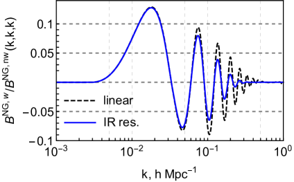
Figure 7: Oscillating contribution in the non-Gaussian bispectrum due to BAO for equilateral configurations at redshift $z=0$. Blue solid (black dashed) lines show the results with (without) IR resummation. The separation scale $k_{S}=0.2\,h$/Mpc.

One can show that the final formula (D.11) is also valid in the squeezed limit. An extra contribution coming from the daisy dressing of the non-Gaussian wiggly vertex $\bar{\Gamma}_{n}^{\prime NG,\,{\rm w}}$ and corresponding to the second term in Eq. (6.35) in fact cancels against the contribution of the fish diagram composed of the wiggly Gaussian and non-wiggly non-Gaussian vertices,

$$\fmffile{BAOfish}\fmfgraph*(120,50)\fmfpen{thick}\fmfkeep{1loop_{2}}\fmfleft{l1,l2}\fmfright{r1}\fmfv{d.sh=circle,d.filled=shaded,d.si=7thick,label=,l.a=135,l.d=.05w}{v1}\fmf{plain,label={\bf q}_{0},l.side=right}{l1,v1}\fmf{plain,label={\bf k},l.side=left}{l2,v1}\fmf{plain,tension=1.2,label=-{\bf k}-{\bf q}_{0}}{v2,r1}\fmf{plain,left=0.9,tension=0.5,label=}{v1,v2}\fmf{plain,left=0.9,tension=0.5,label=,l.side=left}{v2,v1}\fmfv{decor.shape=pentagram,decor.filled=empty,decor.size=7thick,label=,l.a=120,l.d=.07w}{v2}\fmfposition$$ (D.13)

We leave the proof of this cancellation to the reader.

The effect of IR resummation on the BAO feature in the non-Gaussian bispectrum is illustrated in Fig. 7. We see a clear damping of the oscillations due to large bulk flows. Of course, even apart from the damping, the contribution of BAO in the linear bispectrum is at most several per cent. Given the current constraints on non-Gaussianity, measuring this feature appears unfeasible even with futuristic surveys.

References

- [1] A. Schneider et al., “Matter power spectrum and the challenge of percent accuracy,” JCAP 1604, no. 04, 047 (2016) [arXiv:1503.05920 [astro-ph.CO]].
- [2] F. Bernardeau, S. Colombi, E. Gaztanaga and R. Scoccimarro, “Large scale structure of the universe and cosmological perturbation theory,” Phys. Rept. 367, 1 (2002) [astro-ph/0112551].
- [3] R. Scoccimarro, E. Sefusatti and M. Zaldarriaga, “Probing primordial non-Gaussianity with large - scale structure,” Phys. Rev. D 69, 103513 (2004) [astro-ph/0312286].
- [4] A. Taruya, K. Koyama and T. Matsubara, “Signature of Primordial Non-Gaussianity on Matter Power Spectrum,” Phys. Rev. D 78, 123534 (2008) [arXiv:0808.4085 [astro-ph]].
- [5] E. Sefusatti, “1-loop Perturbative Corrections to the Matter and Galaxy Bispectrum with non-Gaussian Initial Conditions,” Phys. Rev. D 80, 123002 (2009) [arXiv:0905.0717 [astro-ph.CO]].
- [6] V. Assassi, D. Baumann and F. Schmidt, “Galaxy Bias and Primordial Non-Gaussianity,” JCAP 1512, no. 12, 043 (2015) [arXiv:1510.03723 [astro-ph.CO]].
- [7] V. Desjacques, D. Jeong and F. Schmidt, “Large-Scale Galaxy Bias,” Phys. Rept. 733, 1 (2018) [arXiv:1611.09787 [astro-ph.CO]].
- [8] D. Baumann, A. Nicolis, L. Senatore and M. Zaldarriaga, “Cosmological Non-Linearities as an Effective Fluid,” JCAP 1207, 051 (2012) [arXiv:1004.2488 [astro-ph.CO]].
- [9] J. J. M. Carrasco, M. P. Hertzberg and L. Senatore, “The Effective Field Theory of Cosmological Large Scale Structures,” JHEP 1209, 082 (2012) [arXiv:1206.2926 [astro-ph.CO]].
- [10] V. Assassi, D. Baumann, E. Pajer, Y. Welling and D. van der Woude, “Effective theory of large-scale structure with primordial non-Gaussianity,” JCAP 1511, 024 (2015) [arXiv:1505.06668 [astro-ph.CO]].
- [11] T. Baldauf, M. Mirbabayi, M. Simonovic and M. Zaldarriaga, “LSS constraints with controlled theoretical uncertainties,” arXiv:1602.00674 [astro-ph.CO].
- [12] Y. Welling, D. van der Woude and E. Pajer, “Lifting Primordial Non-Gaussianity Above the Noise,” JCAP 1608, no. 08, 044 (2016) [arXiv:1605.06426 [astro-ph.CO]].
- [13] T. Sprenger, M. Archidiacono, T. Brinckmann, S. Clesse and J. Lesgourgues, “Cosmology in the era of Euclid and the Square Kilometre Array,” JCAP 1902, 047 (2019) [arXiv:1801.08331 [astro-ph.CO]].
- [14] D. Karagiannis, A. Lazanu, M. Liguori, A. Raccanelli, N. Bartolo and L. Verde, “Constraining primordial non-Gaussianity with bispectrum and power spectrum from upcoming optical and radio surveys,” Mon. Not. Roy. Astron. Soc. 478, no. 1, 1341 (2018) [arXiv:1801.09280 [astro-ph.CO]].
- [15] R. de Putter, “Primordial physics from large-scale structure beyond the power spectrum,” arXiv:1802.06762 [astro-ph.CO].
- [16] E. Silverstein and A. Westphal, “Monodromy in the CMB: Gravity Waves and String Inflation,” Phys. Rev. D 78, 106003 (2008) [arXiv:0803.3085 [hep-th]].
- [17] R. Flauger, L. McAllister, E. Pajer, A. Westphal and G. Xu, “Oscillations in the CMB from Axion Monodromy Inflation,” JCAP 1006, 009 (2010) [arXiv:0907.2916 [hep-th]].
- [18] R. Flauger and E. Pajer, “Resonant Non-Gaussianity,” JCAP 1101, 017 (2011) [arXiv:1002.0833 [hep-th]].
- [19] N. Arkani-Hamed and J. Maldacena, “Cosmological Collider Physics,” arXiv:1503.08043 [hep-th].
- [20] H. Lee, D. Baumann and G. L. Pimentel, “Non-Gaussianity as a Particle Detector,” JHEP 1612, 040 (2016) [arXiv:1607.03735 [hep-th]].
- [21] N. Arkani-Hamed, D. Baumann, H. Lee and G. L. Pimentel, “The Cosmological Bootstrap: Inflationary Correlators from Symmetries and Singularities,” arXiv:1811.00024 [hep-th].
- [22] P. A. R. Ade et al. [Planck Collaboration], “Planck 2015 results. XX. Constraints on inflation,” Astron. Astrophys. 594, A20 (2016) [arXiv:1502.02114 [astro-ph.CO]].
- [23] Y. Akrami et al. [Planck Collaboration], “Planck 2018 results. X. Constraints on inflation,” arXiv:1807.06211 [astro-ph.CO].
- [24] X. Chen, C. Dvorkin, Z. Huang, M. H. Namjoo and L. Verde, “The Future of Primordial Features with Large-Scale Structure Surveys,” JCAP 1611, no. 11, 014 (2016) [arXiv:1605.09365 [astro-ph.CO]].
- [25] M. Ballardini, F. Finelli, C. Fedeli and L. Moscardini, “Probing primordial features with future galaxy surveys,” JCAP 1610, 041 (2016) Erratum: [JCAP 1804, no. 04, E01 (2018)] [arXiv:1606.03747 [astro-ph.CO]].
- [26] G. A. Palma, D. Sapone and S. Sypsas, “Constraints on inflation with LSS surveys: features in the primordial power spectrum,” JCAP 1806, no. 06, 004 (2018) [arXiv:1710.02570 [astro-ph.CO]].
- [27] X. Chen, P. D. Meerburg and M. Munchmeyer, “The Future of Primordial Features with 21 cm Tomography,” JCAP 1609, no. 09, 023 (2016) [arXiv:1605.09364 [astro-ph.CO]].
- [28] Y. Xu, J. Hamann and X. Chen, “Precise measurements of inflationary features with 21 cm observations,” Phys. Rev. D 94, no. 12, 123518 (2016) [arXiv:1607.00817 [astro-ph.CO]].
- [29] A. Slosar et al., “Scratches from the Past: Inflationary Archaeology through Features in the Power Spectrum of Primordial Fluctuations,” arXiv:1903.09883 [astro-ph.CO].
- [30] Y. Akrami et al. [Planck Collaboration], “Planck 2018 results. IX. Constraints on primordial non-Gaussianity,” arXiv:1905.05697 [astro-ph.CO].
- [31] G. Cabass, E. Pajer and F. Schmidt, “Imprints of Oscillatory Bispectra on Galaxy Clustering,” JCAP 1809, no. 09, 003 (2018) [arXiv:1804.07295 [astro-ph.CO]].
- [32] A. Moradinezhad Dizgah, H. Lee, J. B. Munoz and C. Dvorkin, “Galaxy Bispectrum from Massive Spinning Particles,” JCAP 1805, no. 05, 013 (2018) [arXiv:1801.07265 [astro-ph.CO]].
- [33] P. D. Meerburg, M. Munchmeyer, J. B. Munoz and X. Chen, “Prospects for Cosmological Collider Physics,” JCAP 1703, no. 03, 050 (2017) [arXiv:1610.06559 [astro-ph.CO]].
- [34] Z. Vlah, U. Seljak, M. Y. Chu and Y. Feng, “Perturbation theory, effective field theory, and oscillations in the power spectrum,” JCAP 1603, no. 03, 057 (2016) [arXiv:1509.02120 [astro-ph.CO]].
- [35] D. Blas, M. Garny, M. M. Ivanov and S. Sibiryakov, “Time-Sliced Perturbation Theory for Large Scale Structure I: General Formalism,” JCAP 1607, no. 07, 052 (2016) [arXiv:1512.05807 [astro-ph.CO]].
- [36] D. Blas, M. Garny, M. M. Ivanov and S. Sibiryakov, “Time-Sliced Perturbation Theory II: Baryon Acoustic Oscillations and Infrared Resummation,” JCAP 1607, no. 07, 028 (2016) [arXiv:1605.02149 [astro-ph.CO]].
- [37] M. M. Ivanov and S. Sibiryakov, “Infrared Resummation for Biased Tracers in Redshift Space,” JCAP 1807, no. 07, 053 (2018) [arXiv:1804.05080 [astro-ph.CO]].
- [38] N. Aghanim et al. [Planck Collaboration], “Planck 2018 results. VI. Cosmological parameters,” arXiv:1807.06209 [astro-ph.CO].
- [39] D. Blas, J. Lesgourgues and T. Tram, “The Cosmic Linear Anisotropy Solving System (CLASS) II: Approximation schemes,” JCAP 1107, 034 (2011) [arXiv:1104.2933 [astro-ph.CO]].
- [40] D. Babich, P. Creminelli and M. Zaldarriaga, “The Shape of non-Gaussianities,” JCAP 0408, 009 (2004) [astro-ph/0405356].
- [41] N. Bartolo, S. Matarrese and A. Riotto, “Nongaussianity from inflation,” Phys. Rev. D 65, 103505 (2002) [hep-ph/0112261].
- [42] P. Creminelli, “On non-Gaussianities in single-field inflation,” JCAP 0310, 003 (2003) [astro-ph/0306122].
- [43] L. Senatore, K. M. Smith and M. Zaldarriaga, “Non-Gaussianities in Single Field Inflation and their Optimal Limits from the WMAP 5-year Data,” JCAP 1001, 028 (2010) [arXiv:0905.3746 [astro-ph.CO]].
- [44] M. Pietroni, “Flowing with Time: a New Approach to Nonlinear Cosmological Perturbations,” JCAP 0810, 036 (2008) [arXiv:0806.0971 [astro-ph]].
- [45] A. L. Fitzpatrick, L. Senatore and M. Zaldarriaga, “Contributions to the dark matter 3-Point function from the radiation era,” JCAP 1005, 004 (2010) [arXiv:0902.2814 [astro-ph.CO]].
- [46] Z. Huang and F. Vernizzi, “The full CMB temperature bispectrum from single-field inflation,” Phys. Rev. D 89, no. 2, 021302 (2014) [arXiv:1311.6105 [astro-ph.CO]].
- [47] T. Tram, C. Fidler, R. Crittenden, K. Koyama, G. W. Pettinari and D. Wands, “The Intrinsic Matter Bispectrum in CDM,” JCAP 1605, no. 05, 058 (2016) [arXiv:1602.05933 [astro-ph.CO]].
- [48] D. Blas, M. Garny and T. Konstandin, “On the non-linear scale of cosmological perturbation theory,” JCAP 1309, 024 (2013) [arXiv:1304.1546 [astro-ph.CO]].
- [49] A. Vasudevan, “Primordial Non-Gaussianities in the Time-Sliced Perturbation Theory of Cosmological Structure Formation,” MSc Thesis, RWTH Aachen University, Aachen Germany (2017).
- [50] R. Scoccimarro and J. Frieman, “Loop corrections in nonlinear cosmological perturbation theory,” Astrophys. J. Suppl. 105, 37 (1996) [astro-ph/9509047].
- [51] A. Kehagias and A. Riotto, “Symmetries and Consistency Relations in the Large Scale Structure of the Universe,” Nucl. Phys. B 873, 514 (2013) [arXiv:1302.0130 [astro-ph.CO]].
- [52] M. Peloso and M. Pietroni, “Galilean invariance and the consistency relation for the nonlinear squeezed bispectrum of large scale structure,” JCAP 1305, 031 (2013) [arXiv:1302.0223 [astro-ph.CO]].
- [53] P. Creminelli, J. Norena, M. Simonović and F. Vernizzi, “Single-Field Consistency Relations of Large Scale Structure,” JCAP 1312, 025 (2013) [arXiv:1309.3557 [astro-ph.CO]].
- [54] B. Horn, L. Hui and X. Xiao, “Soft-Pion Theorems for Large Scale Structure,” JCAP 1409, no. 09, 044 (2014) [arXiv:1406.0842 [hep-th]].
- [55] T. Baldauf, M. Mirbabayi, M. Simonovic and M. Zaldarriaga, “Equivalence Principle and the Baryon Acoustic Peak,” Phys. Rev. D 92, no. 4, 043514 (2015) [arXiv:1504.04366 [astro-ph.CO]].
- [56] J. M. Maldacena, “Non-Gaussian features of primordial fluctuations in single field inflationary models,” JHEP 0305, 013 (2003) [astro-ph/0210603].
- [57] E. Pajer, F. Schmidt and M. Zaldarriaga, “The Observed Squeezed Limit of Cosmological Three-Point Functions,” Phys. Rev. D 88, no. 8, 083502 (2013) [arXiv:1305.0824 [astro-ph.CO]].
- [58] G. Cabass, E. Pajer and F. Schmidt, “How Gaussian can our Universe be?,” JCAP 1701, no. 01, 003 (2017) [arXiv:1612.00033 [hep-th]].
- [59] D. J. Eisenstein, H. j. Seo, E. Sirko and D. Spergel, Astrophys. J. 664, 675 (2007) [astro-ph/0604362].
- [60] N. Padmanabhan, M. White and J. D. Cohn, Phys. Rev. D 79, 063523 (2009) [arXiv:0812.2905 [astro-ph]].
- [61] F. Beutler, M. Biagetti, D. Green, A. Slosar and B. Wallisch, arXiv:1906.08758 [astro-ph.CO].