Transit modelling of selected Kepler systems

Abstract

This paper employs a simple model, considering just geometry and linear or quadratic limb darkening, to fit Kepler transit data via a Markov Chain Monte Carlo (MCMC) methodology for Kepler-1b, 5b, 8b, 12b, 77b, 428b, 491b, 699b, 706b, and 730b. Additional fits were made of the systems using the more sophisticated modeller Winfitter, which gives results in general agreement with the simpler model. Analysis of data with longer integration times showed biasing of the derived parameters, as expected from the literature, leading to larger estimates for radii and reducing estimates of the system inclination.

Keywords optimization; exoplanets; light curve analysis

1 Introduction

Since the first discoveries of planets orbiting other stars over two decades ago, many thousands have been discovered (see Pollacco et al. (2006) and Rice (2014) for reviews). Transits, where the planet passes in between its host star and an observer’s line of sight leading to a dimming which can be modelled, have been the main data source for exoplanet detection to date. The Kepler mission is currently the major provider of such data (see Borucki et al., 2003 and 2011, for further information on this mission). The Kepler Science Center has managed the organization of these data for scientific users, being readily available from the NASA Exoplanet Archive (NEA: http://exoplanetarchive.ipac.caltech.edu, Akeson et al., 2013).

This paper makes use of data from the NEA and focuses on recovering the transit parameters with their uncertainties for exoplanets. We proceeded with these steps:

• Build a simple planetary transit light curve model using the Python programming language.

• Fit the light curve model on five “known” (or test) exoplanet data-sets (Kepler 1b, Kepler 5b, Kepler 8b, Kepler 12b and Kepler 77b), for which multiple published results from transit modelling exist. Compare the parameter estimates with the literature, to gain reassurance that our model produces results similar to those from other methods, ideally within confidence ranges. These fits would be based on the Levenberg-Marquadt algorithm, and provide starting parameter estimates for Hamiltonian Monte Carlo (HMC) optimizations. Then compare the results with those published elsewhere or as listed on the NEA website.

• Fit the light curve model on systems without multiple fits in the literature, using Markov Chain Monte Carlo (MCMC) procedures to obtain independent estimates and uncertainties of the parameters for the systems. Kepler 428b, Kepler 491b, Kepler 699b, Kepler 706b, and Kepler 730b were selected on the basis of having deep transits and uncomplicated light curves (e.g., visual inspection showed no obvious ellipticity, strong reflections, single planet, etc.) Morton et al.’s (2016) probabilistic validation method tests all conceivable astrophysical false positive scenarios, producing estimates whether the cause of a transit candidate signal is likely due to planet transiting the presumed target star. Morton estimates for these systems a planetary source at the 100% level, bar for Kepler-699 with a probability of 99.1%. MCMC model fit results are available for these systems at the NEA (Thompson et al, 2018; Hoffman & Rowe, 2017), which use quadratic limb darkening parameters taken from Claret & Bloemen (2011) and so not included as optimisable parameters. This paper’s model attempts to fit limb darkening.

• Check these five systems with a second algorithm, Winfitter (Rhodes & Budding, 2014), which uses a Radau model that considers ellipticity and reflection (Kopal, 1959). The program performs optimisation by a modified Levenberg-Marquardt technique and estimates error with Hessian inverse matrix (Budding et al., 2016a, b).

• Analyse possible sources of errors and suggest future improvements.

This project is similar to that described by Ji et al (2017), with this paper being a partial extension of the work described by Ji, where further background may be found.

2 Simple Model

The model was simple, essentially equivalent to that of Mandel & Agol (2002), using the following parameters: the planet’s orbital radius $a$, the stellar radius $r_{s}$, the planet’s radius $r_{p}$, orbital inclination $i$, and initially the linear limb darkening coefficient $u$. Additional parameters $U$ and offset were included to adjust the reference points of the flux axis and phase axis respectively. An assumption of Gaussian noise was included into the model, allowing a fit estimate to be made (‘sigma’ in the following discussions). The adoption of circular orbits is a limitation of this model, along with the use of linear limb darkening and the ‘small planet’ approximation (see, e.g., Nutzman et al., 2009). Inclination follows the usual convention adopted by eclipsing binary light curve models, e.g. $90\degree$ when in our line of sight.

We started with linear limb darkening coefficients, given the discussion of Budding et al. (2016) on the complexity of limb darkening models and the information content of the modelled data. Other authors such as Kipping (2010) and Csizmadia et al. (2013) note the difficulty of extracting limb darkening coefficients from light curves. Nevertheless, following the initial linear term MCMC fits we extended the model to quadratic limb darkening to see if we could obtain co-efficients, and whether these were in line with Claret & Bloemen (2011).

	Current Study				Esteves et al.
System	${r_{p}}/{r_{s}}$	${a}/{r_{s}}$	$i$	$u$	${r_{p}}/{r_{s}}$	${a}/{r_{s}}$	$i$	$u$
Kepler-1b	0.1277	7.8629	83.8115	0.665	$0.12539_{(-0.00035)}^{(+0.00049)}$	$7.903_{(-0.016)}^{(+0.019)}$	$83.872_{(-0.018)}^{(+0.020)}$	0.598
Kepler-5b	0.0795	6.1844	87.1027	0.443	$0.079965_{(-0.000071)}^{(+0.000087)}$	$6.450_{(-0.025)}^{(+0.021)}$	$89.14_{(-0.32)}^{(+0.44)}$	0.561
Kepler-8b	0.0957	6.6869	83.6664	0.529	$0.095751_{(-0.00023)}^{(+0.00019)}$	$6.854_{(-0.017)}^{(+0.018)}$	$83.978_{(-0.033)}^{(+0.036)}$	0.567
Kepler-12b	0.1191	7.7614	87.5911	0.486	$0.118867_{(-0.000094)}^{(+0.000085)}$	$8.019_{(-0.013)}^{(+0.014)}$	$88.796_{(-0.074)}^{(+0.088)}$	0.589

Table 1 : Parameter values from LM fits. The NEA results are from Esteves al. (2015). The LM methodology only provided point estimates and not ‘uncertainties’, explaining the need for a following step to be a method such as boot-strapping or MCMC to better understand the accuracy of the estimates. The LM results do not overlap with the confidence intervals of Esteves et al., although without uncertainties for this paper’s results only a conclusion of general agreement between the two methods can be made.

3 Levenberg-Marquadt (LM) Fits

The LM algorithm can be seen as a combination of the steepest gradient algorithm and the Newton algorithm (Li et al., 2017), providing point estimates. Short cadence data from Quarter 1 were downloaded for Kepler-1b, 5b, and 8b from the NEA website and folded using the given (NEA) system periods. Quarter 2 short cadence data were used for Kepler-12b. Results for LM fits assuming only linear limb darkening are given in table 1, and compared with results from the NEA. These are all similar (as well as to other studies such as Ji et al., 2017, and Budding et al., 2016a,b), lending confidence to our procedures. The LM results were used as starting parameterisations for the subsequent Monte Carlo modelling. The scipy.optimize.leastsq method was used for these optimisations (Jones et al, 2001).

4 MCMC

In probability theory, a Markov chain is a sequence of random variables $\theta^{1},\theta^{2},...,$ in which, for any $t$, the distribution of $\theta^{t}$, even given all previous $\theta$’s, depends only on the most recent value, $\theta^{t-1}$. Markov chain simulation is a general method that draws values of $\theta$ from approximate distributions, and then improves the draws at each subsequent step to better approximate the target posterior distribution, $p(\theta|y)$ (where $y$ is the dependent variable). The sampling is done sequentially, such that the sampled draws form a Markov chain (Gelman et al., 2009). We used the Hamiltonian Monte Carlo (HMC) algorithm, which suppresses the local random walk behaviour of the classic Metropolis-Hasting algorithm, allowing faster exploration of the target distribution. The algorithm was implemented using the pystan package in Python.

System	p ($r_{p}/r_{s}$)	or ($r_{s}/a$)	u	cos(i)	$\sigma$ (x $10^{-6}$)	T
Kepler-1b	0.1275 $\pm$ 0.0004	0.128 $\pm$ 0.003	0.636 $\pm$ 0.003	0.1084 $\pm$ 0.0005	42 $\pm$ 4	100
Kepler-5b	0.0794 $\pm$ 0.0003	0.157 $\pm$ 0.002	0.431 $\pm$ 0.013	0.0301 $\pm$ 0.0129	112 $\pm$ 9	80
Kepler-8b	0.0958 $\pm$ 0.0018	0.147 $\pm$ 0.007	0.614 $\pm$ 0.085	0.1062 $\pm$ 0.0011	910 $\pm$ 40	200
Kepler-12b	0.1191 $\pm$ 0.0005	0.129 $\pm$ 0.002	0.486 $\pm$ 0.015	0.0417 $\pm$ 0.0060	160 $\pm$ 30	20
Kepler-77b	0.0994 $\pm$ 0.0004	0.107 $\pm$ 0.008	0.575 $\pm$ 0.017	0.0471 $\pm$ 0.0021	196 $\pm$ 10	200
Kepler-428b	0.1467 $\pm$ 0.0002	0.119 $\pm$ 0.001	0.717 $\pm$ 0.011	0.0843 $\pm$ 0.0006	42 $\pm$ 8	150
Kepler-491b	0.0818 $\pm$ 0.0003	0.094 $\pm$ 0.001	0.599 $\pm$ 0.010	0.0489 $\pm$ 0.0022	86 $\pm$ 6	100
Kepler-699b	0.1644 $\pm$ 0.0005	0.024 $\pm$ 0.001	0.722 $\pm$ 0.067	0.0192 $\pm$ 0.0002	61 $\pm$ 2	80
Kepler-706b	0.1423 $\pm$ 0.0004	0.016 $\pm$ 0.001	0.649 $\pm$ 0.011	0.0092 $\pm$ 0.0002	40 $\pm$ 13	80
Kepler-730b	0.0850 $\pm$ 0.0003	0.116 $\pm$ 0.001	0.618 $\pm$ 0.018	0.0871 $\pm$ 0.0018	52 $\pm$ 6	200

Table 2 : Parameter values from the linear limb darkening MCMC fits. One standard deviation ‘errors’ are given (as $\sigma$). ‘p’ is the planetary radius $r_{p}$ divided by the stellar radius $r_{s}$ , ‘or’ the stellar radius $r_{s}$ divided by $a$ (the orbital semi-major axis), ‘u’ the linear limb darkening, and ‘cos(i)’ the cosine of the orbital inclination. ‘T’ is the number of steps, in thousands, taken following burn-in periods. The chains were not thinned, given the ACF results discussed in the paper body. Howarth (2011) gives 0.5364 as the linear limb darkening coefficient for Kepler-5 and 0.5850 for Kepler-8. The second value is close to this paper’s, but the first is well outside reasonable ‘errors’ based on the derived standard deviations.

System	p ($r_{p}/r_{s}$)	or ($r_{s}/a$)	u	cos(i)	$\sigma$ (x $10^{-6}$)
Kepler-5b	0.0790 $\pm$ 0.0021	0.1592 $\pm$ 0.0177	0.477 $\pm$ 0.034	0.0393 $\pm$ 0.0005	64.5
Kepler-77b	0.0994 $\pm$ 0.0016	0.1019 $\pm$ 0.0039	0.516 $\pm$ 0.038	0.0333 $\pm$ 0.0003	88.3
Kepler-428b	0.1465 $\pm$ 0.0002	0.1170 $\pm$ 0.0011	0.683 $\pm$ 0.011	0.0810 $\pm$ 0.0006	41.8
Kepler-491b	0.0816 $\pm$ 0.0012	0.0861 $\pm$ 0.0030	0.594 $\pm$ 0.029	0.0311 $\pm$ 0.0004	50.7
Kepler-699b	0.1646 $\pm$ 0.0004	0.0237 $\pm$ 0.0001	0.644 $\pm$ 0.137	0.0187 $\pm$ 0.0002	62.4
Kepler-706b	0.1424 $\pm$ 0.0003	0.0162 $\pm$ 0.0001	0.627 $\pm$ 0.012	0.0085 $\pm$ 0.0002	43.2
Kepler-730b	0.0846 $\pm$ 0.0003	0.1117 $\pm$ 0.0007	0.615 $\pm$ 0.017	0.0805 $\pm$ 0.0011	51.6

Table 3 : Parameter values from WinFitter fits. Labels are as described at Table 2.

Cadence	${r_{p}}/{r_{s}}$	${a}/{r_{s}}$	$i(deg)$	$u$
Short	[0.0878, 0.0912]	[0.0878, 0.0912]	[87.331, 89.156]	[0.565, 0.650]
Long	[0.0880, 0.0911]	[0.1306, 0.1462]	[82.849, 84.043]	[0.399, 0.714]

Table 4 : Comparison of optimal parameters for long and short cadence data for Kepler-491b

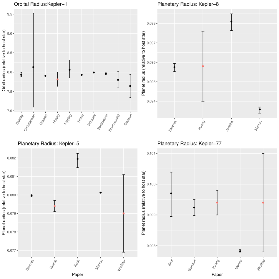
Fig. 1 : Sample comparisons of parameters derived in this study (using MCMC as described in the body) against the literature. Papers are referred to by their primary author: Barclay et al (2012), Christiansen et al (2011), Endl et al. (2014), Esteves et al (2015), Gandolfi et al. (2013) Holczer et al. (2016), Holman et al. (2007), Kipping & Bakos (2011), Koch et al. (2010), Morton et al. (2016), Raetz (et al. (2014), Schroter et al (2012), Torres et al. (2008), and Turner et al. (2016). Huang (this paper) used 68% confidence intervals from their MCMC fits as estimates of uncertainty, colorblue as does Winfitter (based on examination of the error matrix, the inverse of the Hessian). Errors for the other papers are as those papers reported them.

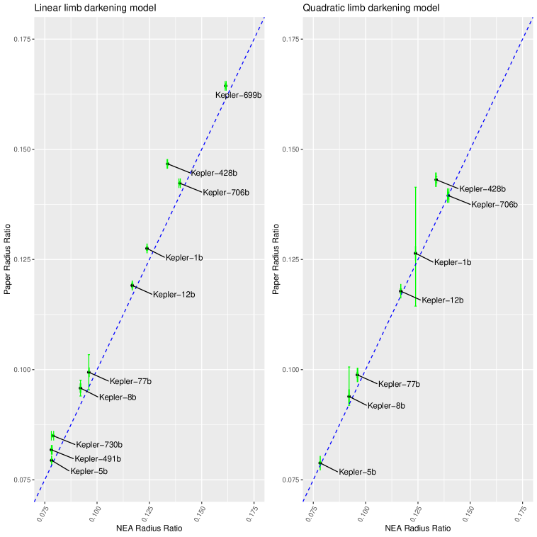
Fig. 2 : Comparison of the planet to star radius from this paper (vertical axis) with those from the NEA MCMC fits (horizontal axis). The chart on the left is based in the linear limb darkening model, and on the right the quadratic limb darkening. The blue dotted lines are those of perfect agreement, not the lines of best fit from linear regressions.

To reduce the impact of the starting values, we discarded the first half of each sequence before carrying out any analysis and inference. This practice of discarding early iterations in Markov chain simulation is referred to as discarding the ‘warm-up’.

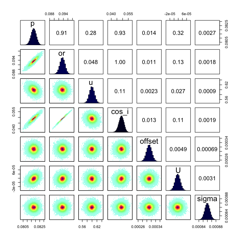
Fig. 3 : Correlation plot for Kepler 491 short cadence dataset, based on MCMC modelling using 4 chains. The density plots (in the lower left of the diagram) plot these 100,000 points for each parameter of the light curve model. ‘p’ is the planetary radius $r_{p}$ divided by the stellar radius $r_{s}$ , ‘or’ the stellar radius $r_{s}$ divided by $a$ (the orbital semi-major axis), ‘u’ the linear limb darkening, ‘cos_i’ the cosine of the orbital inclination, ‘offset’ the phase offset of the folded light curve, ‘U’ the overall flux adjustment, and ‘sigma’ the Gaussian noise in the binned data (1 standard deviation). The histograms along the diagonal show the “error” of the derived parameters (as well as the maximum likelihood), while the numbers in the upper right of the diagram are the correlation coefficients between pairs of the parameters.

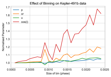
Fig. 4 : Binning test using Kepler 491 short cadence dataset.

System	p ($r_{p}/r_{s}$)	or ($r_{s}/a$)	$u_{1}$	$u_{2}$	cos(i)	$\sigma$ (x $10^{-6}$)
Kepler-1b	$0.1264_{-0.0012}^{+0.0015}$	$0.1296_{-0.0011}^{+0.0016}$	$0.33_{-0.22}^{+0.17}$	$0.40_{-0.21}^{+0.25}$	$0.110_{-0.01}^{+0.02}$	44
Kepler-5b	0.0788 $\pm$ 0.0003	0.156 $\pm$ 0.014	0.31 $\pm$ 0.04	0.26 $\pm$ 0.09	0.019 $\pm$ 0.011	107
Kepler-8b	$0.0939_{-0.0020}^{+0.0067}$	$0.1470_{-0.0065}^{+0.0156}$	$0.30_{-0.16}^{+0.54}$	$0.77_{-0.25}^{+0.20}$	$0.104_{-0.01}^{+0.06}$	919
Kepler-12b	0.1178 $\pm$ 0.0005	0.128 $\pm$ 0.001	0.38 $\pm$ 0.03	0.25 $\pm$ 0.07	0.037 $\pm$ 0.004	103
Kepler-77b	0.0988 $\pm$ 0.0006	0.106 $\pm$ 0.001	0.47 $\pm$ 0.06	0.19 $\pm$ 0.11	0.045 $\pm$ 0.002	197
Kepler-428b	0.1431 $\pm$ 0.0007	0.122 $\pm$ 0.001	0.22 $\pm$ 0.09	0.80 $\pm$ 0.15	0.0871 $\pm$ 0.0009	135
Kepler-706b	0.1395 $\pm$ 0.0008	0.0166 $\pm$ 0.0001	0.34 $\pm$ 0.08	0.61 $\pm$ 0.14	0.0091 $\pm$ 0.0003	42

Table 5 : Parameter values from the quadratic limb darkening MCMC fits. Post-warmup chains were 200,000 steps. $u_{1}$ is the first coefficient in quadratic limb darkening, and $u_{2}$ the second. The errors for Kepler-1b and 8b were not Gaussian, so median values are reported with differences to upper and lower quartiles to give indication of spread. Kipping (2010) reported $u_{1}$ values of 0.38 and 0.14 for his fits to Kepler short and long cadence Kepler-1b data respectively, and $u_{2}$ values of 0.20 and 0.46 for the two data sets. Unfortunately the large derived errors in this study (for short cadence data) make a comparison meaningless, although emphasizing his comment on the difficulty of deriving limb darkening coefficients from these data. Kepler-699b failed to stabilise at a physical solution, pushing both $u_{1}$ and $u_{2}$ to zero and p towards one. Kepler-491b and 730b also failed, indicating full indeterminacy for $u_{2}$.

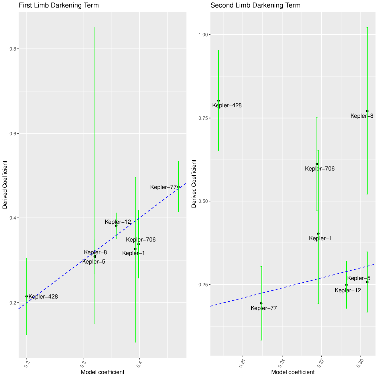
Fig. 5 : Comparison between the quadratic limb darkening terms derived from the MCMC model fits and those of Claret & Bloemen (2011). The latter are used as fixed input by Thompson et al (2018) and Hoffman & Rowe (2017) in their MCMC fits. The blue coloured dotted lines are those of perfect agreement between the data sets (slope 1, intercept 0), showing that the first term is in better agreement better the two data sets than the second term.

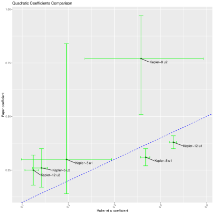
Fig. 6 : Comparison of Muller et al (2013) quadratic limb darkening coefficients for systems in common with current paper. Muller et al. modelled short cadence Kepler data. The estimates do not fall (within errors) on the marked line (slope 1, intercept 0), which would indicate agreement. ‘u1’ is the first quadratic term, and ‘u2’ the second.

4.1 MCMC Results

The data for the MCMC test systems were the same as used in the LM fits. Table 2 summarises the results for the systems, where the model included linear limb darkening. Figure 1 shows a sample of comparisons for system parameters from this table compared with literature results, showing a general agreement that we took as encouraging. It also clearly demonstrates the frequently different estimates for uncertainties. The left hand plot of Figure 2 plots the ratio of the planet to stellar radii for the NEA MCMC fits against those from this paper’s linear limb darkening models. A linear regression indicates a 2.1% difference in the estimates (this paper giving systematically larger radii), although with a 3.9% standard error in this estimate. The intercept was 0.002 $\pm$ 0.004. These results should be contrasted with those in Figure 1, which shows similar magnitude range in scatter across studies.

We therefore moved to the step of modelling systems without published MCMC analyses including limb darkening as free parameters. 1600 days of Kepler data starting BJD 2454833 were folded using the NEA published period and modelling was carried out for systems Kepler-428b, 699-b, and 706b. Kepler-491b data covered 160 days from BJD 2455333.

Kepler data are available in two cadences, short cadence and long cadence. Each cadence is composed of multiple 6.02-s exposures with associated 0.52-s readout times (Gilliland et al., 2011). There is a longer time interval between observations for long and short cadence data which means there are 30 times more short cadence than long cadence data points in a quarter.

Long cadence data were used for Kepler-428b, 699b, 706b, and 730b. Short cadence data were used for Kepler-491b, as these were available for this system, but not for the other three. The chains all converged well. The trace plots exhibited rapid up-and-down variations with no long term trends, indicating good mixing and that the Markov chains explored well the posterior distributions. The ACF (auto-correlation function) plots all decayed rapidly for each modelled parameter. $\hat{R}$ statistics were all close to 1, suggesting good convergence. Results are given in Table 2. As discussed in Brooks & Gelman (1998), if $\hat{R}$ is less than 1.2 then the chains are approximately converged. Figure 3 is an example correlation plot from this modelling, and representative for the modelled systems.

To confirm the results from the simple model used in this paper, we used Winfitter (see, e.g., Budding et al., 2016) and its more detailed fitting function to model the same data. Table 3 presents the results for key parameters, which are in good agreement with the simple model estimates, lending confidence in them.

Kepler-491b had both long and short cadence data available, allowing us to explore whether the derived parameters were affected by the implicit data binning. Table 4 summarises the interval estimates given by the HMC algorithm for short and long cadence datasets. When long cadence data are used to fit our light curve model, the estimates for the parameters $\frac{r_{s}}{a}$ and $\frac{r_{p}}{r_{s}}$ are high while the estimate for the parameter $i$ is considerably reduced. This suggests that the use of long cadence dataset may systematically overestimate the radii of a planet and host star, while underestimating the planetary inclination.

We further investigated this binning effect using the Kepler 491b short cadence dataset. Figure 4 shows the percentage change in the point estimates of the transit parameters given by the HMC algorithm for various bin widths, relative to the point estimates derived from the first bin width (0.0001 phase bin). We can see that when the bin width increases, the derived radii $r_{p}$ and $r_{s}$ become larger while the inclination $i$ becomes smaller (derived parameters $\frac{r_{p}}{r_{s}}$, $\frac{r_{s}}{a}$, $\cos(i)$ increase as bin width increases). This point was made by Kipping (2010), who recommended to first compute the transit model at a finer time sampling, and then integrate the “supersampled” model over the observed integration time before comparing it to the data. The present analysis has independently confirmed the underlying point, but rather than rework the model’s approximations for different sampling bins we call attention to the observable effects of finite sampling in the residuals, since this might be associated with some physical effect, such as abnormal limb-darkening.

Murphy (2012) commented that ‘the short cadence data are almost always better than the long cadence data’. Our analysis confirms this observation, at least for the systems we modelled.

We have only tested the impact of long cadence data by one system. For other planetary systems having similar transit times and orbital periods as Kepler-491b, we can expect a similar impact of the cadence value on the parameters. For planetary systems that have longer transit durations, the use of long cadence data may not be of such importance.

Finally, we returned to the matter of including quadratic limb darkening (see Table 5), including it into the MCMC fits. Convergence could not be obtained for all systems (e.g., 491, 699, and 730), suggesting we were attempting to extract ‘too much’ information from the data.

The right hand plot of Figure 2 compares the radii ratios for the systems with quadratic limb darkening fits in this paper against the NEA estimates. The difference for the other systems was within approximately one percent and within the combined error of the estimates (but outside the formal errors for the radii given by the linear limb darkening fits). There is poor agreement between the models of Claret & Bloemen (2011) and the fit results for the $u_{2}$ limb darkening values, but better for $u_{1}$ (see Figure 5).

Howarth (2011) presented simulations where use of the linear law led to systematic errors of up to 4% in radius estimates, but negligible error introduced when the quadratic law was used. This study finds a mean increase of 1.4 $\pm$ 0.8% increase in the planetary radii ratios using linear limb darkening to those using quadratic, but this difference was driven by Kepler 428 and 706 with their larger differences.

5 Winfitter Quadratic Limb Darkening

We then attempted Winfitter fits including quadratic limb darkening. Winfitter evaluates the $\chi^{2}$ Hessian (see, for example, Bevington, 1969) in the vicinity of the derived minimum. Inspection of this matrix, and in particular its eigenvalues and eigenvectors, gives insights into parameter determinancy and interdependence. The Hessian can be inverted to yield an error matrix. A positive definite matrix indicates a determinate, ‘unique’ solution. This makes it possible to determine which of the adjustable parameters are likely to allow well-defined optimal values, as well as providing an error range for the optimized parameters. Further information on how Winfitter evaluates the information content of data may be found in Banks & Budding (1990). Further details on Winfitter and its usage may be found in Budding & Najim (1980), Budding & Zeilik (1987), and Budding & Demircan (2007).

Only the fits for Kepler-5 and Kepler-77 were positive definite when quadratic limb darkening was included into the model, indicating that the information content of the data was being exceeded. Inclination tended to be the variable ‘breaking’, which would be inline with its high correlation with radii (see, for example, Figure 3). However Winfitter indicated large errors for the limb darkening coefficients for these two ‘successful’ systems: $u_{1}=-0.01\pm 0.26$ and $u_{2}=0.30\pm 0.20$ for Kepler-5 $u_{1}=0.30\pm 0.46$ and $u_{2}=0.13\pm 0.32$ for Kepler-77. These large errors are symptomatic of near breakdown of determinacy. All fits with linear limb darkening were positive definite.

We do not expect it too surprising that quadratic limb darkening coefficients could not be reliably ‘solved’ for the long integration data sets with the current methods, nor that it would be challenging with the short integration Kepler data. For example, previous MCMC optimisations by Ji et al (2017) had met the same problems with Kepler-1 and Southworth (2009) had commented that “….the linear law is adequate for most of the datasets studied in this work (particularly those from longer wavelengths)” in his study of exoplanet transit light curves.

Putting to one side our information limit concerns, we also tried a two stage fitting approach to see what the effect on radii of quadratic limb darkening would be compared to linear. We first fitted the ratio of the radii, the limb darkening coefficients, the stellar radius, and the inclination (as well as adjustments in flux and time), followed by removing the radii from the parameters optimised in a second fit. This led to planetary radius estimates from the quadratic fits that were systematically biased compared to those from the linear limb darkening fits (by $0.991\pm 0.004$) and in stellar radii by $1.050\pm 0.018$. We do not put much weight on these ratios, given the small data set. There was poor agreement between the derived limb darkening parameters and those of Claret & Bloemen (2011). The Pearson correlation coefficients were $-0.44$ for $u_{1}$ and $-0.31$ for $u_{2}$.

Attempts to determine limb darkening coefficients are important, as exoplanet transit light curves provide a ‘laboratory’, hopefully providing data that can be used to test and refine stellar models (see also Csizmadia et al, 2013). Higher signal to noise data would be ideal for these tests, particularly given the correlation between limb darkening and our key variable of interest, the exoplanet radius.

6 Conclusions

Kepler-1b, 5b, 8b, 12b, 77b, 428b, 491b, 699b, 706b, and 730b were analyzed with two approaches: an MCMC one based on Mandel & Agol (2002) and the other Winfitter on Kopal (1959). These systems do not show any significant level of tidal and rotational distortion, for instance, by visual inspection of the light curves. The coefficients for gravity-darkening and stellar reflectivity were not optimised in the majority of the Winfitter fits, bar for Kepler-699, 706, and 730 where the reflection coefficient was found to be zero ($\pm$ 0.0001, $\pm$ 0.0002, and $\pm$ 0.0001 respectively). Further details on how ellipticity is included into the model may be found in Kopal (1959). In general, for these systems the Winfitter results are in good agreement with the parameter values from the MCMC fits. However the fractional stellar radius and inclination of the Kepler-491 system are different to that from the MCMC fits. There is a relationship or correlation between the two variables (see Fig 3), so while it is disappointing that there is a difference in the estimates it can be understood.

We have three major conclusions from this study:

• We note difficulty in consistent error estimates across methodologies, as given in the literature. As shown in Fig 1, there can be a wide range in error estimates for the same system, from many multiples larger than the estimates from the MCMC and Winfitter fits of this paper, to many multiples less. However it is encouraging that the point estimates are in reasonable agreement. Regardless, care will need to be taken with meta-analyses based on the literature to avoid over-interpretation, particularly for systems with perhaps only one published solution.

• It appears difficult to derive limb darkening coefficients through fitting, noting that we should not have used the long cadence data for such modelling without compensating for the integration times. However, Csizmadia et al. (2013) recommend trying to fit these parameters, noting that some authors have highly different observed limb darkening coefficients from the theoretical predictions (e.g., Claret, 2009; Kipping & Bakos, 2011, Barros et al., 2009). It is hoped that similar MCMC fittings could provide useful data to test stellar models (see e.g., Figure 6 for a comparison of common systems in one such paper with the current paper) and the reliability of such estimates. As Muller et al (2013) note, the upcoming PLATO and JWST missions, along with the current TESS mission, should provide high signal to noise data that will allow deeper investigations of limb darkening including any diversity with effective temperature etc. Southworth (2008, 2009, 2010, 2011, 2012) provides an interesting self-consistent survey with careful consideration of errors, worthy of emulation.

• Consideration of integration periods will prove important for analysis of some systems where observations have long integration times compared to transit ingress or egress. Examples could include the TESS mission for selected stars observed with 30-minute time sampling in the full-frame images (FFIs, see Bouma et al., 2017, for further information on TESS). Such binning will, naturally, be increasingly important for transits where the integration times are significant fractions of the total transit time. Flux measurements during the ingress and egress periods will be ‘smeared out’, leading to wider estimates of the planetary radius, as we have seen in this study. A simple model, as we have used in this paper, will lead to systematic biases in the derived parameters unless compensation is made for the longer integration times. We intend to add this feature into later work with Winfitter on long integration data.

  We did not explore thoroughly in this paper a detailed comparison of the formal errors produced by the MCMC and Winfitter methodologies, as believe this is worthy of a more detailed follow-up study. We intend to implement MCMC as the optimisation technique for the Winfitter model, allowing deeper examination of the errors estimated by this methodology. Winfitter is not only a more sophisticated model, for instance including relevant proximity effects (such as radiative interaction, tidal and rotational distortions) as well as orbital ellipticity with the methodology to include simple modeling of starspots. It is much faster in computer runtimes than MCMC, and if it can be shown that its error estimates are comparable to those from MCMC, it could be a useful tool for large scale studies across multiple exoplanet systems. A comparison of the formal errors for the systems in this paper is inconclusive — for instance, Winfitter tended to underestimate (in comparison with the MCMC model) errors in $\cos{i}$, was generally larger in $u$, and mixed in stellar and planetary radii. We intend to widen the data set, using short integration time data.

7 Acknowledgements

This research has made use of the NASA Exoplanet Archive, which is operated by the California Institute of Technology, under contract with the National Aeronautics and Space Administration via the Exoplanet Exploration Program. It is a pleasure to acknowledge additional help and encouragement from the National University of Singapore (NUS), particularly through Prof. Lim Tiong Wee of the Department of Statistics and Applied Probability. This paper reports results from an undergraduate student project at NUS, in that department. Winfitter may be sourced from https://michaelrhodesbyu.weebly.com/astronomy.html. We thank the referees of this paper for their helpful comments, which helped improve the paper.

References

- akeson (2013) Akeson, R.L., Chen, X., Ciardi, D., Crane, M., Good, J., Harbut, M., Jackson, E., Kane, S.R., Laity, A.C., Leifer, S., Lynn, M., McElroy, D. L., Papin, M., Plavchan, P., Ramirez, S.V., Rey, R., von Braun, K., Wittman, M. , Abajian, M., Ali, B., Beichman, C., Beekley, A., Berriman, G.B., Berukoff, S., Bryden, G., Chan, B., Groom, S., Lau, C., Payne, A. N., Regelson, M., Saucedo, M., Schmitz, M., Stauffer, J., Wyatt, P., & Zhang, A., PASP, 125, 989, 2013
- Banks (1990) Banks, T., & Budding, E., 1990, Ap&SS, 167, 221
- Barclay (2012) Barclay, T., Huber, D., Rowe, J.F., Fortney, J.J., Morley, C.V., Quintana, E.V., Fabrcky, D.C., Barentsen, G., Bloemen, S., Christiansen, J.L., Demory, B-O, Fulton, B.J., Jenkins, J.M., Mullally, F., Ragozzine, D., Seader, S.E., Shporer, A., Tenebaum, P., & Thompson, S.E., 2012 Ap. J, 761(1), 53
- Barrosi (2012) Barros, S. C. C., Pollacco, D. L., Gibson, N. P., et al., 2012, MNRAS, 419, 1248
- Bevingtoni (1969) Bevington, P. R., 1969, Data Reduction and Error Analysis for the Physical Sciences , McGraw-Hill, New York
- Borucki (2003) Borucki, W.J., et al. (14 authors), 2003, in Scientific Frontiers in Research on Extrasolar Planets, Eds. D. Deming and S. Seager, ASP Conf. Ser. 294, 427
- (7) Borucki, W.J., et al. (69 authors), 2011, ApJ, 736, 19
- (8) Bouma, L. G., Winn, Joshua N., Kosiarek, Jacobi, et al. 2017, pre-print (arXiv170508891B)
- (9) Brooks, S., & Gelman, A., 1997, J. Comput. Graph Stat., 7(4), 434
- (10) Budding, E., & Najim, N. N., 1980, Ap & SS, 72, 369.
- (11) Budding, E., & Demircan, O., 2007, Introduction of Astronomical Photometry, Cambridge University Press, Cambridge.
- (12) Budding, E., & Zeilik, M., 1987, Ap. J., 319, 827
- Budding (2016a) Budding, E., Püsküllü, Ç., Rhodes, M.D., Demircan, O., & Erdem, A., 2016a, Ap&SS, 361, 17
- Budding (2016b) Budding, E., Rhodes, M.D., Püsküllü, Ç., Ji, Y., Erdem, A., & Banks, T., 2016b, Ap&SS, 361, 346
- (15) Claret, A., 2009, A&A, 506, 1335
- (16) Claret, A., & Bloemen, S., 2011, A&A, 529, 75
- Csizmadia (2013) Csizmadia, Sz., Pasternacki, Th., Dreyer, C., Cabrera, J., Erikson, A., & Rauer, H., 2013, A&A, 549, A9
- Budding (2007) Budding, E., & Demircan, O., 2007, Introduction to Astronomical Photometry, CUP
- Budding (2016a) Budding, E., Püsküllü, Ç., Rhodes, M.D., Demircan, O., & Erdem, A., 2016a, Ap&SS, 361, 17
- Budding (2016b) Budding, E., Rhodes, M.D., Püsküllü, Ç., Ji, Y., Erdem, A., & Banks, T., 2016b, Ap&SS, 361, 346
- Charbonneau (1999) Charbonneau, D., Noyes, R.W., Korzennik, S.G., Nisenson, P., Jha, S., Vogt, S.S., & Kibrick, R.I., 1999, ApJ, 527, 445
- Christiansen (2011) Christiansen, J.L., Ballard, S., Charbonneau, D., Deming, D., Holman, M.J., Madhusudhan, N., Seager, S., Wellnitz, D.D., Barry, R.K., Livengood, T.A., Hewagama, R., Hampton, D.L., Lisse, C.M., & A’Hearn, M.F., 2011, Ap. J., 726, 94
- Endl (2014) Endl, M., Caldwell, D. A., Barclay, T., et al., 2014, Ap. J., 795, 151
- Esteves (2015) Esteves, L.J., De Mooij, E.,J.W., & Jayawardhana, R., 2015, Ap. J, 804(2), 28
- gandolfi (2015) Gandolfi, D., Parviainen, H., Fridlund, M., et al., 2013, A & A, 557, 74
- gelman (2009) Gelman, A., Carlin, J.B., Stern, H.S., & Rubin, D.B., Bayesian Data Analysis — Second Edition, 2009, Chapman & Hall/CRC.
- Giliand (2011) Gilliland, R. L., Chaplin, W. J., Dunham, E. W., et al., 2011, ApJS, 197, 6.
-
Hoffman (2017)
Hoffman, K. L., & Rowe, J. F., 2017,
Uniform Modeling of KOIs: MCMC Notes for Data Release 25,
KSCI-19113-001 (https://exoplanetarchive.ipac.caltech.edu/
docs/KSCI-19113-001.pdf) - Holczer (2016) Holczer, T., Mazeh, T., Nachmani, G., Jontof-Hutter, D., Ford, E. B., Fabrycky, D., Ragozzine, D., Kane, M., & Steffen, J. H., 2016, Ap. J SS, 225, 9
- Holman (2007) Holman, M.J., Winn, J.N., Latham, D.W., O’Donovan, F. T., Charbonneau, D., Torres, G., Sozzetti, A., Fernadez, J., & Everett, M.E., 2007, Ap. J., 664, 1185.
- Howarth (2011) Howarth, I.D., 2011, MNRAS, 418, 1165
- Ji (2017) Ji, Y., Banks, T., Budding, E., & Rhodes, M.D., 2017, Ap&SS, 362, 12
- Jones (2001) Jones, E., Oliphant, E., Peterson, P., et al., 2001, SciPy: Open Source Scientific Tools for Python. Accessed Dec 12, 2017 from http://www.scipy.org/
- Kipping (2010) Kipping, D., 2010, MNRAS, 408 (3), 1758
- Kipping (2017) Kipping, D., & Bakos, G., 2011, Ap. J., 733, 36
- Koch (2010) Koch, D. G., Borucki, W. J., Rowe, J. F., et al, 2010, Ap. J Letters, 713, 131
- Kopal (1959) Kopal, Z., 1959, Close Binary Systems, London, Chapman & Hall.
- Li (2017) Li, J., Zheng, W. X., Gu, J., & Hua, L., 2017, Journal of the Franklin Institute, 354(1), 316
- Mandel (202) Mandel, K., & Agol, E., 2002, Astrophys. J., 580, 171
- Morton (2016) Morton, T.D., Bryson, S.T., Coughlin, J.L., Rowe, J.F., Ravichandran, G., Petihura, E.A., Haas, M.R.,& Batalha, N. M., 2016, Ap. J., 822, 86
- Muller (2013) Muller, H. M., Huber, K.F., Czesla, S., Wolter, U., & Schmitt, J. H. M. M., 2013., A&A 560, A112
- Murphy (2012) Murphy, S.,J., 2012, MNRAS, 422(1), 665
- Nutzman (2009) Nutzman, P., Charbonneau, D., Winn, J. N., Knutson, H.A., Fortney, J.J., Holman, M. J., & Agol, E., Ap. J., 692, 229, 2009
- Pollacco (2006) Pollacco, D.L., et al., 2006, Publ. Astron. Soc. Pac., 118, 1407
- Puskullu (2018) Puskullu, C., & Soydugan, F., 2018, Canadian Journal of Physics, 96, 685.
- Raetz (2014) Raetz, St., Maciejeski, G., Ginski, Ch., et al, 2014, MNRAS, 444, 1351
- Rice (2014) Rice, K., 2014, Challenges, 5, 296
- Rhodes (2014) Rhodes, M. and Budding, E., 2014, Ap&SS, 351, 451
- Schroter (2012) Schroter, S., Schmitt, J. H. M. M., & Muller, H. M., 2012, A & A, 539, 97
- Southworth (2008) Southworth, J., 2008, MNRAS, 386, 1644
- Southworth (2009) Southworth, J., 2009, MNRAS, 394, 272
- Southworth (2010) Southworth, J., 2010, MNRAS, 408, 1689
- Southworth (2011) Southworth, J., 2011, MNRAS, 417, 2166
- Southworth (2012) Southworth, J., 2012, MNRAS, 426, 1291
- Thompson (2018) Thompson, S. E., Coughlin, J. L., Hoffman, K., Mullally, F., at al., 2018, ApJS, 235, 38
- Torres (2008) Torres, G., Winn, J. N., & Holman, M. J., 2008, Ap. J, 677, 1324
- Turner (2016) Turner, J.D., Perason, K.A., Biddle, L. I., et al., 2016, MNRAS, 459, 789