Optimal measurement network of pairwise differences

Abstract

When both the difference between two quantities and their individual values can be measured or computationally predicted, multiple quantities can be determined from the measurements or predictions of select individual quantities and select pairwise differences. These measurements and predictions form a network connecting the quantities through their differences. Here, I analyze the optimization of such networks, where the trace ($A$-optimal), the largest eigenvalue ($E$-optimal), or the determinant ($D$-optimal) of the covariance matrix associated with the estimated quantities are minimized with respect to the allocation of the measurement (or computational) cost to different measurements (or predictions). My statistical analysis of the performance of such optimal measurement networks–based on large sets of simulated data–suggests that they substantially accelerate the determination of the quantities, and that they may be useful in applications such as the computational prediction of binding free energies of candidate drug molecules.

I Introduction

It is quite common in a scientific study that multiple quantities are to be determined from the measurements of their individual values and their pairwise differences. (I will refer to both experimental measurements and computational predictions as measurements unless otherwise distinguished.) Compared to measuring only the individual quantities, including measurements of pairwise differences may substantially improve the statistical precision in the estimated quantities. This is especially true when the statistical uncertainties in the measurements of the differences are much lower than that in the measurements of the individual quantities, e.g., when the differential value between two quantities lies within the detection range of the experimental technique but the individual values are outside the detection limit.

The statistical uncertainty associated with measuring a quantity or a pairwise difference depends on the resources allocated to the measurement, i.e. the number of repetitions in the case of experimental measurements or the number of uncorrelated data points sampled in the case of computational predictions. Given fixed total measurement resources (i.e. cost), optimal allocation of the resources to different measurements may substantially improve the overall statistical precision–characterized by the covariance matrix–of the estimated quantities Stephen Boyd (2004); Pukelsheim (2006).

An important example that may benefit from such optimal resource allocations is the computational prediction of the binding affinities of a set of molecules for a target receptor of pharmaceutical interest. Binding free energy calculations have demonstrated sufficient accuracy Harder et al. (2016) and are increasingly adopted in the pharmaceutical industry as an effective method to rank and select candidate molecules in many drug discovery projects Wang et al. (2015). The binding free energy of an individual molecule can be computed by the technique of absolute binding free energy calculations Boresch et al. (2003); Mobley et al. (2007); Woo and Roux (2005); Aldeghi et al. (2015), and the difference between the binding free energies of any two molecules can be computed by the technique of relative binding free energy calculations Cournia et al. (2017); Tembre and Cammon (1984); Radmer and Kollman (1997); Wang et al. (2015). Optimal estimators for individual absolute or relative binding free energy calculations have been developed Bennett (1976); Shirts and Chodera (2008). At fixed computational cost, the statistical errors of free energy calculations are bound by the thermodynamic length between the thermodynamic end states Shenfeld et al. (2009). Typically, the end states are more dissimilar in absolute binding free energy calculations than in relative binding free energy calculations. As a result, the statistical errors in the former are often substantially larger than those in the latter given the same amount of computational cost.

The binding free energies of all the molecules in the set can be estimated from the appropriate combinations of the predicted individual values and the predicted pairwise differences (see below). Optimal allocation of computational resources to different absolute and relative binding free energy calculations may lead to improved efficiency in predicting the binding free energies of a set of molecules. Past effort aimed at providing redundancy and consistency checks in the calculations Liu et al. (2013). How to minimize the overall statistical error in the estimated binding free energies, however, remains an unaddressed question.

Here, I apply the mathematical results from optimal experimental designs Stephen Boyd (2004); Pukelsheim (2006) to the special case of optimizing the allocations of measurement resources to the measurements of individual quantities and their pairwise differences, so as to minimize the overall statistical error in the estimated quantities. Specifically, I consider three types of optimization: 1) the $A$-optimal, which minimizes the trace of the covariance matrix and hence the total variance, 2) the $D$-optimal, which minimizes the determinant of the covariance matrix and hence the volume of the confidence ellipsoid for a fixed confidence level, and 3) the $E$-optimal, which minimizes the largest eigenvalue of the covariance matrix and hence the diameter of the confidence ellipsoid. The $A$-optimal and the $D$-optimal are found by iterative numerical minimization. For the $E$-optimal, I present a new mathematical theorem that enables the minimization to be solved by construction. I characterize the statistical performance of such optimizations in terms of the reduction in the statistical error in the estimated quantities at fixed total measurement cost. My results suggest that optimal designs of the measurements can substantially reduce the statistical error in the estimated quantities, allowing the same statistical precision (characterized by the total statistical error) to be achieved at–on average–less than half the measurement cost when compared to naive allocations. The Python code for generating the optimal designs is made available as free open source software (https://github.com/forcefield/DiffNet).

II Theory

Suppose that we want to measure a set of quantities $\{x_{i=1,2,\dots,m}\}$. We can either measure each individual quantity $x_{i}$ with the estimator $\hat{x}_{i}=x_{i}+\sigma_{i}$, or the difference between any pair of quantities $x_{i}$ and $x_{j}$ with the estimator $\hat{x}_{ij}=x_{i}-x_{j}+\sigma_{ij}$, where $\sigma_{i}$ and $\sigma_{ij}$ are the respective statistical errors in the measurements. For each measurement $e\in\{i|i=1,2,...,m\}\cup\{(i,j)|i,j=1,2,\dots,m,i\neq j\}$, the statistical variance of the estimate decreases with $n_{e}$–the resource allocated to the measurement–as

$$\sigma_{e}^{2}=s_{e}^{2}/n_{e}$$ (1)

where $s_{e}$ is the statistical fluctuation in the corresponding experimental measurement or computer sampling.

The quantities and the measurements form a network–which I will refer to as the difference network–represented by a graph $\mathcal{G}$ of $m+1$ vertices and $m(m+1)/2$ edges, where the vertices $i=1,2,\dots,m$ stand for the $m$ quantities $\{x_{i}\}$, the edge between vertices $i\neq j>0$ stands for the difference measurement $\hat{x}_{ij}$, and the edge between vertices $0$ and $i>0$ stands for the individual measurement $\hat{x}_{i}$. Two weighted graphs can be derived from $\mathcal{G}$: 1) $\mathcal{G}_{s}$, in which the weight assigned to each edge is the corresponding fluctuation $s_{e}$, and 2) $\mathcal{G}_{n}$, in which the weight is the corresponding number of samples $n_{e}$. I will denote $s_{i,0}=s_{0,i}=s_{i}$ and $n_{i,0}=n_{0,i}=n_{i}$.

For a given set of $\{n_{e}\}$ and the corresponding $\{\sigma_{e}\}$ per Eq. 1, the maximum likelihood estimator for $\{x_{i}\}$ is Stephen Boyd (2004); Pukelsheim (2006); Wang et al. (2013) (assuming that the statistical errors in the measurements follow the normal distribution; see Appendix A for a derivation)

$$\mathbf{F}\cdot\vec{x}=\vec{z}$$ (2)

where

$$z_{i}=\sigma_{i}^{-2}\hat{x}_{i}+\sum_{j\neq i}\sigma_{ij}^{-2}\hat{x}_{ij},$$ (3)

and $\mathbf{F}$ is the Fisher information matrix:

$$F_{ij}=\left\{\begin{array}[]{rl}\sigma_{i}^{-2}+\sum_{k\neq i}\sigma_{ik}^{-2}&\text{ if }i=j\\ -\sigma_{ij}^{-2}&\text{ if }i\neq j\end{array}\right..$$ (4)

The covariance in the estimates of $\{x_{i}\}$ is given by the inverse of the Fisher information matrix:

$$\mathbf{C}=\mathbf{F}^{-1}$$ (5)

In the classical theory of optimal design of experiments Pukelsheim (2006), three objectives of minimizations of statistical errors with respect to $\{n_{e}\}$ are commonly sought:

• $A$-optimal: minimize $\mathrm{tr}(\mathbf{C})$,

• $D$-optimal: minimize $\ln\det(\mathbf{C})$,

• $E$-optimal: minimize $||\mathbf{C}||_{2}$,

where $\mathrm{tr}(\mathbf{C})$ denotes the trace of the matrix $\mathbf{C}$, $\det(\mathbf{C})$ denotes the determinant of $\mathbf{C}$, and $||\mathbf{C}||_{2}$ denotes the spectral norm–or, equivalently, the largest eigenvalue–of $\mathbf{C}$, subject to the constraints of non-negativity

$$n_{e}\geq 0,$$ (6)

and of total fixed measurement cost

$$\sum_{e}n_{e}=\sum_{i}n_{i}+\sum_{i<j}n_{ij}=N.$$ (7)

Although $\{n_{e}\}$ are integers, the above minimizations are more conveniently performed if $\{n_{e}\}$ are allowed to be real numbers. They can then be rounded to integers (see Appendix. B). This is a reasonable approximation when $N\gg m(m+1)/2$. This condition is usually satisfied in sampling-based computational predictions such as binding free energy calculations, because in such cases $N$ is the total number of independent sampling points, which can be in the range of tens of millions. Automated experiments permitting large numbers of repetitions may also satisfy this condition.

All three objectives are convex functions of $\{n_{e}\}$ (see Appendix C), and the minimization can be performed by standard algorithms in convex optimization Stephen Boyd (2004). For the $A$-optimal design, the minimization can be solved as a semidefinite programming problem (SDP) (see Appendix D).

For the $E$-optimal design, the minimization can be similarly cast as an SDP. But for the difference network, I present the following theorem (see Appendix E for proof), which allows the minimization problem to be solved by construction, with a fixed time complexity of $O(m^{2})$ and space complexity of $O(m)$, and which, to my knowledge, has not appeared in any previous publication.

Theorem 1

Let $E_{i}$ be the shortest path from vertex 0 to vertex $i$ in the graph $\mathcal{G}_{s}$ (i.e., the path with the smallest $\sum_{e\in E_{i}}s_{e}$), and $E=\cup_{i}E_{i}$ be the tree rooted at vertex 0 from the resulting union. (A tree is a connected acyclic undirected graph.) Denoting $a_{0}=0$ and

$$a_{i}=\sum_{e\in E_{i}}s_{e}\text{ for }i>0,$$ (8)

$||\mathbf{C}(\{n_{e}\})||_{2}$ is minimized by the following set of $\{n_{e}\}$:

$$n_{i\mu_{i}}=Ns_{i\mu_{i}}\sum_{j\in T_{i}}a_{j}\left(\sum_{i}a_{i}^{2}\right)^{-1}$$ (9)

where $T_{i}\subset E$ is the subtree rooted at vertex $i$, and $\mu_{i}$ is the vertex immediately preceding $i$ in the path $E_{i}$ from 0 to $i$.

The shortest paths $\{E_{i}\}$ can be constructed by the single-source-multiple-destination Dijkstra algorithm (see, e.g., Ref. Kurt Mehlhorn, 2008), which guarantees that $E=\cup_{i}E_{i}$ is a tree. The $E$-optimal by construction is substantially faster than by minimization using SDP: for random $\{s_{e}\}$ drawn uniformly in the interval $(1,5)$, the speedup of the former over the latter (implemented in CVXOPT Andersen et al. ) is $\sim 400\times$ for $m=10$ and $\sim 3700\times$ for $m=50$. In Appendix F, I suggest a special class of difference networks in which the $A$- and the $D$-optimals may also be solved by construction.

Often, there is a cost $\tau_{e}$ associated with generating each sampling point in the estimator $\hat{x}_{e}$, and the total cost is $\sum_{e}n_{e}\tau_{e}=N$. We can, however, introduce $n_{e}^{\dagger}=n_{e}\tau_{e}$, and $s_{e}^{\dagger}=s_{e}\tau_{e}^{1/2}$, and solve the same problem as above for $n_{e}^{\dagger}$, with the parameters $s_{e}^{\dagger}$.

III Results

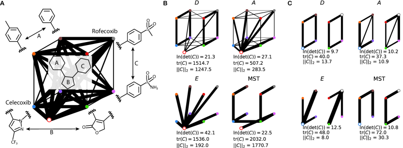
Figure 1: Optimal allocation of computational sampling to the binding free energy calculations for COX-2 inhibitors. A The 8 inhibitors are generated by different combinations of 3 rings, with 2 different options for each ring. The weighted graph $\mathcal{G}_{s}$ is shown. Each filled vertex represents an inhibitor. The edge between any two such vertices $i$ and $j$ represents the relative binding free energy calculation between inhibitors $i$ and $j$, and the thickness of the edge is proportional to the corresponding $s_{ij}$. The edge between the unfilled vertex at the bottom and a vertex $i$ represents the absolute binding free energy calculation of inhibitor $i$, and its thickness is proportional to $s_{i}$. B The $D$-, $A$-, and $E$-optimals of the corresponding difference network, where the thickness of each edge is proportional $n_{e}$ according to the optimal allocations. C The optimals when the binding free energies of Celecoxib and Rofecoxib are known and used as references, and only relative binding free energy calculations are used to computed the binding free energies of the other 6 inhibitors. For comparison, the minimum spanning tree (MST) of $\mathcal{G}_{s}$ is also shown, where $n_{e}$ is constant for each edge in the tree.

I first illustrate the optimal difference networks using the example of the calculation of the binding free energies of $m=8$ inhibitors for the COX-2 protein Yamakawa et al. (2014). The optimals depend on the statistical fluctuations $\{s_{e}\}=\{s_{i}|i=1,2,\dots,m\}\cup\{s_{ij}|i,j=1,2,\dots,m,i<j\}$. For illustrative purposes, I set $\{s_{e}\}$ such that $s_{i}$ in the absolute binding free energy calculations is $s_{i}=\zeta\sqrt{h_{i}}$, where $h_{i}$ is the number of heavy atoms in molecule $i$ and $\zeta$ is a constant, and that $s_{ij}$ in the relative binding free energy calculations is $s_{ij}=\zeta\sqrt{\max(h_{ij},h_{ji})}$, where $h_{ij}$ is the number of heavy atoms in molecule $i$ that do not transform into atoms in molecule $j$ in the relative binding free energy calculation of molecules $i$ and $j$. The corresponding $\mathcal{G}_{s}$ is shown in Fig. 1A. In real binding free energy calculations, the $\{s_{e}\}$ depends on both the thermodynamic length between the end states Shenfeld et al. (2009) and the ratio of the relaxation time of relevant motions to the length of the simulation; they have to be determined (approximately) during iterative rounds of binding free energy calculations. The optimal allocations corresponding to my hypothetical $\{s_{e}\}$ are shown in Fig. 1B.

In a typical drug discovery projects, there will be a few molecules whose binding free energies have already been experimentally determined, and, using these molecules as references, relative binding free energy calculations can be used to predict the binding free energies for other similar molecules. The $D$-, $A$-, and $E$-optimals for such relative binding free energy calculations are shown in Fig. 1C for the COX-2 inhibitors, using Celecoxib and Rofecoxib as the reference molecules. Because the $\{s_{e}\}$ values above reflects the assummption that relative binding free energy calculations have substantially lower statistical errors than absolute binding free energy calculations, this network of relative binding free energy calculations–taking advantage of the known binding free energies of the reference molecules–yield much lower overall statistical errors than the previous network in Fig. 1B.

Next, I characterize the statistical performance of the optimal difference networks in comparison to naive choices of $\{n_{e}\}$. The $A$-, $D$-, $E$-optimals and various other naive allocations are applied to randomly generated sets of $\{s_{e}\}$, and the resulting covariance matrices are compared in terms of their traces, determinants, and spectral norms.

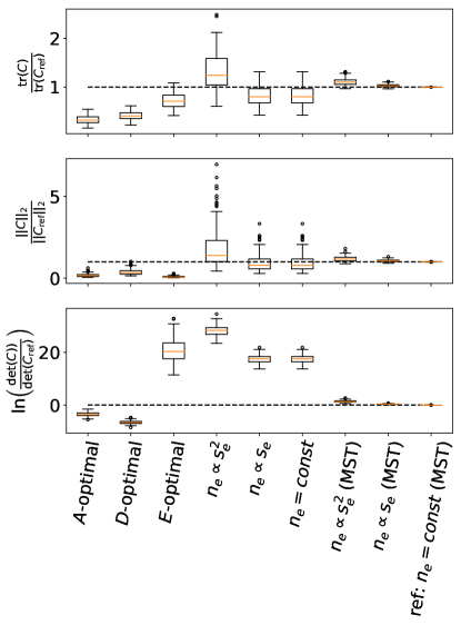
Figure 2: Statistical performance of different allocations. Here $m=30$, $\{s_{ij}\}$ and $\{s_{i}\}$ are uniformly disitrbuted between 1 and 5. As the reference, I chose $n_{e}=const$ for $e\in\text{MST}(\mathcal{G}_{s})$, where $\text{MST}(\mathcal{G}_{s})$ is the minimum spanning tree (MST) of the weighted graph $\mathcal{G}_{s}$. The covariances of the various allocations are computed for $T=200$ randomly generated sets of $\{s_{e}\}$, and the ratios of $\mathrm{tr}(\mathbf{C})$, $||\mathbf{C}||_{2}$, and $\det(\mathbf{C})$ to the corresponding reference values are shown here in boxplots, with the median ratios and the quartiles indicated.

For the sets of random $\{s_{e}\}$ drawn uniformly from the interval of $(1,5)$, the $A$-optimal outperforms all tested schemes of naive allocations by all three criteria ($\mathrm{tr}(\mathbf{C})$, $||\mathbf{C}||_{2}$, and $\det(\mathbf{C})$; it also yields a $||\mathbf{C}||_{2}$ close to that of the $E$-optimal and a $\ln(\det(\mathbf{C}))$ close to that of the $D$-optimal (Fig. 2). Compared to the $D$-optimal, which has the second lowest average $\mathrm{tr}(\mathbf{C})$, the $A$-optimal reduces $\mathrm{tr}(\mathbf{C})$ by a factor of $0.791\pm 0.005$ (i.e. the ratio of $\mathrm{tr}(\mathbf{C})$ for the $A$-optimal to that for the $D$-optimal is $0.791$); compared to the naive allocation $n_{e}\propto s_{e}$, which has the lowest average $\mathrm{tr}(\mathbf{C})$ among the tested naive allocations, the $A$-optimal reduces $\mathrm{tr}(\mathbf{C})$ by a factor of $0.402\pm 0.001$. These observations suggest that the $A$-optimal–which has the simple interpretation of minimizing the total variance of the measured quantities–may be a good default choice in designing difference networks.

The $A$-optimal enables substantial improvements in statistical precision for difference networks with other distributions of $\{s_{e}\}$ as well. For example, in the case where $s_{i}=s_{ij}=\text{constant}$ and $m=30$, the $A$-optimal reduces $\mathrm{tr}(\mathbf{C})$ by a factor of 0.664 compared to the naive allocation $n_{e}\propto s_{e}$; in the case where the relative error is constant (such that $s_{ij}=|s_{i}-s_{j}|$; see Appendix F) and $m=30$ values of $s_{i}$ are drawn randomly from the interval $(0,1)$, the corresponding reduction is by a factor of $0.470\pm 0.001$.

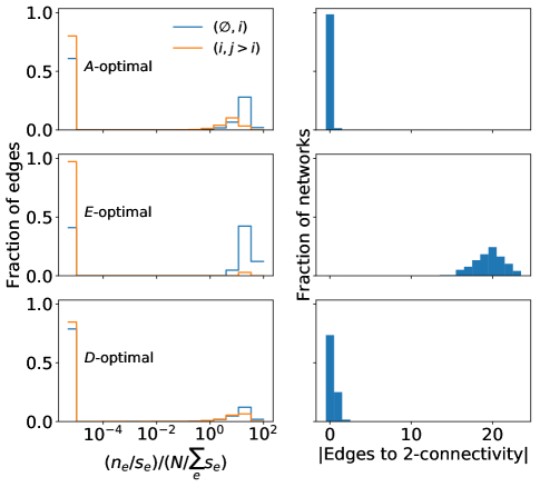
Figure 3: Statistical distributions of $\{n_{e}\}$ in the optimal allocations, for the same random sets of $\{s_{e}\}$ as in Fig. 2. The fractions of edges in the weighted graph $\mathcal{G}_{n}$ with different $n_{e}/s_{e}$ ratios are shown on the left. The right panels show the distributions of the minimum number of edges that need to be added to the graph $\mathcal{G}_{n}$–after eliminating the edges with negligible allocations (determined by $n_{e}/s_{e}/(N/\sum_{e}s_{e})<10^{-2}$)–to make it 2-connected (i.e. there are at least 2 distinct paths connecting any two vertices in $\mathcal{G}_{n}$). The majority of the $A$-optimal networks are 2-connected.

It is desirable that the measurement networks are 2-connected–a $k$-edge-connected subgraph is one that does not become disconnected unless $k$ edges are removed–such that for any two quantities, there are two paths through which their differences can be computed. This allows a self-consistency check: the differences computed both ways should be approximately equal. Such checks can reveal potential measurement errors and outliers. The majority (98.5%) of the $A$-optimal networks are 2-connected, and all of them become 2-connected with the addition of at most 1 edge (Fig. 3). This property of the $A$-optimal allocation also makes it a good choice in designing difference networks.

The $A$- and $D$-optimal networks may be densely connected (the $E$-optimal is a tree hence sparsely connected). For example, in the $A$-optimal allocations for the above randomly generated sets of $\{s_{e}\}$, on average individual measurements are applied to 11.8 of the $m=30$ individual quantities, and difference measurements are applied to 86.7 of the $m(m-1)/2=435$ pairs (Fig. 3). The $A$- and $D$-optimal difference networks for the COX-2 binding free energy calculations (Fig. 1) are also clearly dense. As suggested in Appendix F, however, the $A$- and $D$-optimal networks are trees when $s_{ij}=|s_{i}-s_{j}|$.

Practical considerations–such as the minimum number of samples required in an individual binding free energy calculation to derive meaningful free energy estimates, and how many measurements can be executed in parallel–often make it desirable to limit the number of measurements to include in the difference network, i.e. to limit the number of edges in $\mathcal{G}_{n}$. Appendix H outlines a heuristic approach to designing near-optimal difference networks given the required edge-connectedness $k$ and the number of measurements $M$ (the number of edges in $\mathcal{G}_{n}$ with $n_{e}>0$). The resulting network, $\mathcal{G}_{k,M}$, can be further pruned to eliminate any edge with $n_{e}/N<\epsilon/M$ (e.g., to avoid impractically short binding free energy calculations; $\epsilon$ is a parameter that specifies the cutoff). When applied to the $A$-optimal of the example difference network with randomly generated fluctuations (described in Fig. 2), the $\mathrm{tr}(\mathbf{C})$ of the near-optimal allocation generated by this approach, with $k=2$, $M=3m$, and $\epsilon=0.1$, is on average only $1.10\pm 0.03$ times that of the true optimal.

Design of the optimal difference network requires as input the statistical fluctuations $\{s_{e}\}$ associated with each measurement, which is usually unknown a priori. Thus the application of the optimal difference networks needs to proceed in an iterative manner. Starting with an initial guess of $\{s_{e}\}$ (e.g. the statistical fluctuation in relative or absolute binding free energy calculations may be predicted by a machine-learning model trained on a collection of past free energy calculations), the quantities can be measured with the corresponding optimal network at a small total measurement cost; For any measurement $e$ performed, update $s_{e}$ by the actual statistical variance of the measurement, and re-optimize the network accordingly; Repeat this process at increasingly larger total cost until sufficiently precise estimates of the quantities are reached.

Fig. 4 illustrates this iterative process in the construction of the $A$-optimal for a difference network. In the beginning, $\{s_{e}\}$ were initialized to be random numbers drawn uniformly from the interval of $(0,1)$. In each iteration, $s_{e}$ was updated to be the actual estimate of the fluctuation for any performed measurement $e$ (i.e. $n_{e}>0$), or to be a random number drawn uniformly between the minimum and the maximum of all the estimated fluctuations (i.e. in the interval $(\min_{e^{\prime}|n_{e^{\prime}}>0}(\{s_{e^{\prime}}\}),\max_{e^{\prime}|n_{e^{\prime}}>0}(\{s_{e^{\prime}}\})$) if measurement $e$ has not yet been performed (i.e. $n_{e}=0$). In each iteration, a prescribed total of $\Delta N=\sum_{e}\Delta n_{e}$ additional samples are allocated so as to optimize $\mathrm{tr}(\mathbf{C})$ with respect to $\Delta n_{e}$ (see Appendix G), and $\Delta n_{e}$ are rounded to integers according to Appendix B. In a few iterations the allocation $\{n_{e}(N)\}$ becomes close to the optimal allocation, $\{n_{e}(\infty)\}$, according to the true fluctuations $\{s_{e}^{\infty}\}$. The Kullback-Leiber divergence from $\{n_{e}(N)\}$ to $\{n_{e}(\infty)\}$

$$D_{\text{KL}}[n_{e}(N)||n_{e}(\infty)]=\sum_{e}\frac{n_{e}(N)}{N}\ln\frac{n_{e}(N)}{n_{e}(\infty)}$$ (10)

decreases in each iteration. Correspondingly, the total statistical error in the estimated quantities approaches the true minimum at sufficiently large $N$.

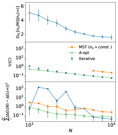
Figure 4: Iterative $A$-optimization of the difference network. Here, the difference network corresponds to that of binding free energy calculations for the eight COX-2 inhibitors, and the true fluctuations $\{s_{e}^{\infty}\}$ are taken to be the same as given in Fig. 1A. Top: The Kullback-Leibler divergence, $D_{\text{KL}}$, between the allocation in each iteration $n_{e}(N)$ and the optimal allocation $n_{e}(\infty)$ according to the true $\{s_{e}^{\infty}\}$ at different total number of samples $N$ after each iteration. Middle: $\mathrm{tr}(C)$ versus $N$ for the iterative optimization, compared to that for the true $A$-optimal and the minimal spanning tree allocation according to $\{s_{e}^{\infty}\}$. Bottom: The square deviation of the estimated free energies $\Delta G_{i}(N)$ after each iteration from the true free energies $\Delta G_{i}(\infty)$. No actual free energy calculations were performed. Instead, $\Delta\Delta G_{ij}$ and their fluctuations $s_{ij}$ are calculated as the average and standard deviations of $n_{ij}$ random numbers drawn from a normal distribution with the mean $\Delta G_{i}(\infty)-\Delta G_{j}(\infty)$ and the standard deviation $s_{ij}^{\infty}$. $\Delta G_{i}$ are estimated from $\Delta\Delta G_{ij}$ and $s_{ij}^{2}/n_{ij}$ using Eq. 2. Iterative optimization quickly approaches the true optimal; at $N=10^{4}$, $\mathrm{tr}(\mathbf{C})$ of the iteratively optimized difference network is practically indistinguishable from that of the true $A$-optimal, and it is $0.249\pm 0.004$ times that of the minimal spanning tree allocation.

IV Discussions

This work explored the application of optimal experimental design to the determination of multiple quantities by the measurements of select individual quantities and select pairwise differences, such as in the computational prediction of binding free energies for candidate drug molecules. A related work was recently published by Yang et al. Yang et al. (2019), in which the authors proposed using discrete $A$- or $D$-optimals to select the pairs of relative binding free energy calculations for predicting the binding free energies of a set of molecules. Whereas Yang et al. addressed the question of between which pairs of molecules relative binding free energy calculations should be performed, given a fixed number of calculations (i.e. $n_{e}=0,1$, under the constraint $\sum_{e}n_{e}=N$, $N$ being the total number of calculations), I addressed here the question of how much sampling should be allocated to the relative binding free energy calculations between each possible pair of molecules, given a fixed total amount of sampling (i.e. $0\leq n_{e}\leq N$, under the constraint $\sum_{e}n_{e}=N$, $N$ being the total number of samples in all the calculations). The expanded domain of $\{n_{e}\}$ in the latter allows additional control in the design of the calculations, which further reduces the resulting statistical errors.

The optimal difference network may help accelerate a variety of scientific inquiries. Improving the statistical precision of binding free energy predictions, for instance, allows better selection of candidate drug molecules in drug discovery projects, as suggested by Yang et al. Yang et al. (2019). The optimal difference network may find immediate use in the parametrization of computational models, where the same set of quantities are computed repeatedly in search for the values of the model parameters that best fit benchmark data. For example, binding free energy calculations for sets of inhibitors binding to their receptor targets Harder et al. (2016) and solvation free energy calculations for a large number of solutes Mobley and Guthrie (2014) are routinely used to test the accuracy of molecular force fields. The increased statistical efficiency conferred by the optimal difference networks will allow faster assessment of the quantitative accuracy of the models and thus shorten their development cycles.

Appendix A Derivation of the estimator and the covariance in the difference network

The set of quantities $\{x_{i}\}$ can be estimated from the measurements $\{\hat{x}_{e}\}$ by the maximum likelihood (ML) estimator. Let $\sigma_{e}^{2}=s_{e}^{2}/n_{e}$ be the variance for the measurement $e$, the likelihood that the measurements produce the set of values $\{\hat{x}_{e}\}$, given the true values of the quantities $\{x_{i}\}$, is

$$L = \prod_{i}(\sqrt{2\pi}\sigma_{i})^{-1}\exp\left(-\frac{(x_{i}-\hat{x}_{i})^{2}}{2\sigma_{i}^{2}}\right)$$ (11)

$$\cdot \prod_{i<j}(\sqrt{2\pi}\sigma_{ij})^{-1}\exp\left(-\frac{(x_{i}-x_{j}-\hat{x}_{ij})^{2}}{2\sigma_{ij}^{2}}\right)$$

The above assumes that the samples in the measurements are independent.

Maximizing $L$ with respect to $\{x_{i}\}$ yields Eq. 2-4. The convariance matrix for the ML estimator is given by the inverse of the Fisher information matrix, hence Eq. 5.

Appendix B Rounding $n_{e}$ to integers

In practice $n_{e}$ need to be rounded to integers that sum to $N$. Let $E_{+}=\{e|n_{e}>0\}$ be the set of measurements requiring samples, and $|E_{+}|$ be the size (or cardinality) of $E_{+}$. One can sort $E_{+}$ by increasing values of $n_{e}$ (such that $n_{e_{j}}$ is the $j$th lowest value), and round up the lowest $k$ values and round down the highest $|E_{+}|-k$ values of $n_{e}$ to the nearest integers. $k$ is chosen such that

$$\sum_{j=1}^{k}\lceil n_{e_{j}}\rceil+\sum_{j=k+1}^{|E_{+}|}\lfloor n_{e_{j}}\rfloor=N,$$ (12)

which yields

$$k=N-\sum_{e\in E_{+}}\lceil n_{e}\rceil-|E_{+}|.$$ (13)

Appendix C Proof of convexity of $\mathrm{tr}(\mathbf{C})$ and $||\mathbf{C}||_{2}$

The objective functions $\mathrm{tr}(\mathbf{C})$, $\det(\mathbf{C})$, and $||\mathbf{C}||_{2}$ have all been previously shown to be convex functions of $\{n_{e}\}$ Stephen Boyd (2004). Here I include simple proofs for the convexity of $\mathrm{tr}(\mathbf{C})$ and $||\mathbf{C}||_{2}$.

The Fisher information matrix $\mathbf{F}=\mathbf{C}^{-1}$ is a linear function of $\{n_{e}\}$. Both $\mathbf{F}$ and $\mathbf{C}$ are symmetric and positive definite. Consider a perturbation $q\mathbf{A}$ to $\mathbf{F}$, where $\mathbf{A}$ is an arbitrary symmetric matrix. The perturbed covariance matrix satisfies

$$\mathbf{C}(q)\cdot(\mathbf{F}+q\mathbf{A})=(\mathbf{F}+q\mathbf{A})\cdot\mathbf{C}(q)=\mathbf{I}$$ (14)

where $\mathbf{I}$ is the identity matrix. Differentiating Eq. 14 with respect to $q$ twice, we have

$$\frac{d^{2}}{dq^{2}}\mathbf{C}(q)=2(\mathbf{A}\cdot\mathbf{C}(q))^{t}\cdot\mathbf{C}(q)\cdot(\mathbf{A}\cdot\mathbf{C}(q))$$ (15)

which is positive definite.

Thus

$$\frac{d^{2}}{dq^{2}}\mathrm{tr}(\mathbf{C}(q))=\mathrm{tr}\left(\frac{d^{2}}{dq^{2}}\mathbf{C}(q)\right)>0$$ (16)

proving the convexity of $\mathrm{tr}(\mathbf{C})$ in $\{n_{e}\}$.

To prove that $||\mathbf{C}||_{2}$ is convex in $\{n_{e}\}$, note that

$$||\mathbf{C}||_{2}=\lambda_{1}(\mathbf{F})^{-1}$$ (17)

where $\lambda_{1}(\mathbf{F})\equiv\min\{\mathrm{eig}(\mathbf{F})\}$ is the smallest eigenvalue of $\mathbf{F}$.

According to the second-order perturbation theory, for the perturbed matrix $\mathbf{F}+q\mathbf{A}$, the corresponding $\lambda_{1}(q)$ is

$$\lambda_{1}(q)=\lambda_{1}(\mathbf{F})+q\mathbf{v}_{1}^{t}\cdot A\cdot\mathbf{v}_{1}+q^{2}\sum_{k=2}^{m}\frac{\left(\mathbf{v}_{k}^{t}\cdot A\cdot\mathbf{v}_{k}\right)^{2}}{\lambda_{1}-\lambda_{k}}+O(q^{3})$$ (18)

where $\lambda_{k}$ is the $k$’th eigenvalue of $\mathbf{F}$ ($k=1,2,\dots,m$), and $\mathbf{v}_{k}$ is the corresponding normalized eigenvector. The second derivative of $\lambda_{1}$ is

$$\frac{d^{2}}{dq^{2}}\lambda_{1}=\sum_{k=2}^{m}\frac{\left(\mathbf{v}_{k}^{t}\cdot A\cdot\mathbf{v}_{k}\right)^{2}}{\lambda_{1}-\lambda_{k}}\leq 0$$ (19)

because $\lambda_{1}\leq\lambda_{k}$,

Thus

$$\frac{d^{2}}{dq^{2}}||\mathbf{C}||_{2}=\frac{2\left(d\lambda_{1}/dq\right)^{2}-\lambda_{1}d^{2}\lambda_{1}/dq^{2}}{\lambda_{1}^{3}}\geq 0$$ (20)

proving the convexity of $||\mathbf{C}||_{2}$ in $\{n_{e}\}$.

Appendix D Semidefinite programming for $A$-optimal design

For the $A$-optimal design, the minimization can be cast by duality as a semidefinite programming problem (SDP):

minimize $$\sum_{i=1}^{m}u_{i}$$ (24)

subject to $$\left(\begin{array}[]{cc}\mathbf{F}(\{n_{e}\})&\mathbf{e}_{i}\\ \mathbf{e}_{i}^{t}&u_{i}\\ \end{array}\right)\succeq 0\text{ for $i=1,2,\dots,m$},$$

$$n_{e}\geq 0\text{ for all }e,\text{ and }\sum_{e}n_{e}=N,$$

where $\mathbf{M}\succeq 0$ signifies that the symmetric matrix $\mathbf{M}$ is positive semidefinite, and $\mathbf{e}_{i}$ is the $i$th unit vector (i.e. $e_{ij}=\delta_{ij}$).

Appendix E Proof that Eq. 9 is the $E$-optimal

The largest eigenvalue of $\mathbf{C}$ is the inverse of the smallest eigenvalue of $\mathbf{F}$ (Eq. 17), so the problem of minimizing $||\mathbf{C}||_{2}$ is equivalent to maximizing the smallest eigenvalue of $\mathbf{F}$:

$$\max_{\{n_{e}\}}{\min\{\mathrm{eig}(\mathbf{F})\}}$$ (25)

The smallest eigenvalue $\lambda_{\text{min}}$ of $\mathbf{F}$ satisfies

$$\lambda_{\text{min}}\leq\vec{a}^{t}\cdot\mathbf{F}\cdot\vec{a}$$ (26)

for all normal vectors $\vec{a},|a|^{2}=1$; the equality holds if and only if $\vec{a}$ is the eigenvector of $\mathbf{F}$ corresponding to $\lambda_{\text{min}}$. Our problem is thus to find

$$\max_{\{n_{e}\}}\min_{|a|^{2}=1}\vec{a}^{t}\cdot\mathbf{F}\cdot\vec{a}$$ (27)

I have

$$\vec{a}^{t}\cdot\mathbf{F}\cdot\vec{a} = \sum_{i}\sigma_{i}^{-2}a_{i}^{2}+\sum_{j\neq i}\sigma_{ij}^{-2}a_{i}^{2}-\sum_{j\neq i}\sigma_{ij}^{-2}a_{i}a_{j}$$ (28)

$$= \sum_{i}\sigma_{i}^{-2}a_{i}^{2}+\sum_{i<j}\sigma_{ij}^{-2}(a_{i}-a_{j})^{2}.$$

Plugging in $\sigma_{e}^{2}=s_{e}^{2}/n_{e}$, I have

$$\vec{a}^{t}\cdot\mathbf{F}\cdot\vec{a}=\sum_{i}\frac{n_{i}a_{i}^{2}}{s_{i}^{2}}+\sum_{i<j}\frac{n_{ij}(a_{i}-a_{j})^{2}}{s_{ij}^{2}}.$$ (29)

Given any vector $\vec{a}$, eq. 29 is maximized with respect to $\{n_{e}\}$ when the only non-zero $n_{e}$’s are the ones corresponding to the largest value of $a_{i}^{2}/s_{i}^{2}$ or $(a_{i}-a_{j})^{2}/s_{ij}^{2}$. There may be degenerate set of $E=\{e\}$ with the largest values:

$$\left.\frac{a_{i}}{s_{i}}\right|_{i\in E}=\left.\frac{|a_{i}-a_{j}|}{s_{ij}}\right|_{ij\in E}=R_{m}\geq\left.\frac{a_{i}}{s_{i}}\right|_{i\not\in E},\left.\frac{|a_{i}-a_{j}|}{s_{ij}}\right|_{ij\not\in E}$$ (30)

and

$$\max_{\{n_{e}\}}{\vec{a}^{t}\cdot\mathbf{F}\cdot\vec{a}}=\sum_{e}n_{e}R_{m}=NR_{m}$$ (31)

The maximimum can be achieved by different values of $\{n_{e}\}$, so long as $n_{e}\neq 0$ only if $e\in E$.

If I can determine a set $E$ and a set of $\{n_{e}^{\ast}\}$ such that $n_{e}^{\ast}\neq 0\iff e\in E$, and the corresponding Fisher information matrix $\mathbf{F}(\{n_{e}^{\ast}\})$ has an eigenvector $\vec{a}$ of the lowest eigenvalue satisfying eq. 30, I have

$$\vec{a}^{t}\cdot\mathbf{F}(\{n_{e}^{\ast}\})\cdot\vec{a}\geq\vec{a}^{t}\cdot\mathbf{F}(\{n_{e}\})\cdot\vec{a}\geq\min_{|a^{\prime}|^{2}=1}\vec{a}^{\prime t}\cdot\mathbf{F}(\{n_{e}\})\cdot\vec{a}^{\prime}$$ (32)

Such a set of $\{n_{e}^{\ast}\}$ would thus be a solution of eq. 27. There may be degenerate solutions of eq. 27 and to our problem.

Next I show how to construct such a set of $\{n_{e}\}$ by constructing its corresponding eigenvector $\vec{a}$ that satisfies eq. 30.

Consider a complete graph $\mathcal{G}_{s}$ consisting of $N+1$ vertices, indexed as $0,1,2,\dots,m$. The edge between the vertex $i$ and the vertex $0$ is assigned weight $s_{i}$, and the edge between the vertex $i$ and the vertex $j$ is assigned weight $s_{ij}$. For each vertex $i\neq 0$, find the shortest path $E_{i}$ from $0$ (i.e., with the smallest sum $a_{i}=\sum_{e\in E_{i}}s_{e}$). We also denote $a_{0}=0$, $s_{i,0}=s_{0,i}=s_{i}$, and $n_{i,0}=n_{0,i}=n_{i}$. I will show that the vector $\vec{a}=\{a_{i=1,2,\dots,m}\}$ is the sought eigenvector, and that $E$ comprises the edges of a tree–rooted at vertex $0$–that is the union of the shortest path to each vertex $i>0$.

Consider the union of $\{E_{i}\}$: $E^{\prime}=\cup_{i}E_{i}$. If there is any loop in $E^{\prime}$, an arbitrary edge in the loop can be removed and the resulting graph will still contain the shortest path from $0$ to every vertex $i$. Thus the tree $E$ can be constructed by removing all the loops in $\cup_{i}E_{i}$. In fact, if $\{E_{i}\}$ are found by the Dijkstra’s algorithm, $\cup_{i}E_{i}$ will not contain any loops. This is taken to be the case below.

First, I prove that $\vec{a}$ and the corresponding $E$ satisfy eq. 30. Clearly

$$\left.\frac{|a_{i}-a_{j}|}{s_{ij}}\right|_{ij\in E}=1$$ (33)

If there exists a pair $i,j$ such that $(a_{i}-a_{j})/s_{ij}>1$, it implies that the shortest path to $i$ is $E_{j}$ followed by edge $ji$, with the sum $a_{j}+s_{ij}<a_{i}$, which is a contradiction.

I can now construct the set $\{n_{e}\}$ so that $\vec{a}$ is the eigenvector of $\mathbf{F}(\{n_{e}\})$, i.e.,

$$\mathbf{F}(\{n_{e}\})\vec{a}=\lambda\vec{a}.$$ (34)

Note that $n_{e}\neq 0$ only if $e\in E$. Denote the set of vertices whose edge to vertex $i$ are in $E$ as $J_{i}$ (which may include the vertex 0), the elements of $\mathbf{F}$ can be written as

$$F_{ii}=\sum_{j\in J_{i}}\frac{n_{ij}}{s_{ij}^{2}}$$ (35)

and

$$F_{ij}=\left\{\begin{array}[]{rl}-\frac{n_{ij}}{s_{ij}^{2}}&\text{if }j\in J_{i}\\ 0&\text{otherwise}\end{array}\right.$$ (36)

and Eq. 34 becomes

$$\lambda a_{i} = F_{ii}a_{i}+\sum_{j\neq i,\ j>0}F_{ij}a_{j}$$ (37)

$$= \sum_{j\in J_{i}}\frac{n_{ij}}{s_{ij}^{2}}a_{i}-\sum_{j\in J_{i}\setminus\{0\}}\frac{n_{ij}}{s_{ij}^{2}}a_{j}$$

$$(\because a_{0}=0)$$

$$= \sum_{j\in J_{i}}\frac{n_{ij}}{s_{ij}^{2}}(a_{i}-a_{j})$$

$$(\because j\in J_{i}\iff(i,j)\in E\Rightarrow|a_{i}-a_{j}|=s_{ij})$$

$$= \sum_{j\in J_{i}}\frac{n_{ij}}{s_{ij}}\mathrm{sgn}(a_{i}-a_{j})$$

Let $\mu_{i}$ be the vertex immediately preceding $i$ in the path $E_{i}$ connecting $0$ to $i$. $j=\mu_{i}$ is the only vertex in $J_{i}$ for which $a_{i}>a_{j}$. Otherwise, let $j^{\prime}$ be another vertex such that $a_{i}>a_{j^{\prime}}$, which implies that the edge $(ij^{\prime})$ cannot be part of $E_{j^{\prime}}$, and thus both $E_{i}$ and $E_{j^{\prime}}\cup{(ij^{\prime})}$ are paths connecting $0$ to $i$, in contradiction to the fact that $E$ is without any loop. Another corollary is that the edge $(i\mu_{i})$ must be in the path $E_{j}$ for every $j$ in the subtree $T_{i}\subset E$ rooted at vertex $i$.

I can write

$$\frac{n_{i\mu_{i}}}{s_{i\mu_{i}}}=\lambda a_{i}+\sum_{j\in J_{i}\setminus\{\mu_{i}\}}\frac{n_{ij}}{s_{ij}}$$ (38)

Eq. 38 can be solved by starting from the leaves of the tree $E$ and working backwards toward vertex $0$. The solution is

$$\frac{n_{i\mu_{i}}}{s_{i\mu_{i}}}=\lambda\sum_{j\in T_{i}}a_{j}$$ (39)

where the sum runs over the set of vertices in the subtree $T_{i}$ rooted at $i$, including $i$ itself.

The eigenvalue $\lambda$ can be determined by applying the constraint $\sum_{e}n_{e}=\sum_{i}n_{i\mu_{i}}=N$.

$$\sum_{i}n_{i\mu_{i}} = \lambda\sum_{i}s_{i\mu_{i}}\sum_{j\in T_{i}}a_{j}$$ (40)

$$= \lambda\sum_{i}(a_{i}-a_{\mu_{i}})\left(a_{i}+\sum_{j\in T_{i}\setminus\{i\}}a_{j}\right)$$

$$= \lambda\left(\sum_{i}a_{i}^{2}+\sum_{i}a_{i}\sum_{j\in T_{i}\setminus\{i\}}a_{j}-\sum_{i}a_{\mu_{i}}\left(a_{i}+\sum_{j\in T_{i}\setminus\{i\}}a_{j}\right)\right)$$

In both $\sum_{i}a_{i}\sum_{j\in T_{i}\setminus\{i\}}a_{j}$ and $\sum_{i}a_{\mu_{i}}(a_{i}+\sum_{j\in T_{i}\setminus\{i\}}a_{j})$, the product $a_{i}a_{j\neq i}$ appears once and only once if and only if $j$ is in the subtree of $T_{i}$ or $i$ is in the subtree of $T_{j}$. This implies that the two sums are equal, and I have

$$N=\sum_{i}n_{i\mu_{i}}=\lambda\sum_{i}a_{i}^{2}$$ (41)

or

$$\lambda=N\left(\sum_{i}a_{i}^{2}\right)^{-1}$$ (42)

To prove that this $\lambda$ in eq. 42 is the smallest eigenvalue of $\mathbf{F}$, I show that it is the largest eigenvalue of the corresponding covariance matrix $\mathbf{C}=\mathbf{F}^{-1}$.

$x_{i}$ is estimated–because $E$ is a tree rooted at $0$–by

$$x_{i}=\sum_{e\in E_{i}}\hat{x}_{e}$$ (43)

thus the covariance between $x_{i}$ and $x_{j}$ is

$$C_{ij} = \sum_{e\in E_{i},e^{\prime}\in E_{j}}\mathrm{cov}(\hat{x}_{e},\hat{x}_{e^{\prime}})$$ (44)

$$= \sum_{e\in E_{i}\cap E_{j}}\sigma_{e}^{2}=\sum_{e\in E_{i}\cap E_{j}}\frac{s_{e}^{2}}{n_{e}}$$

Without loss of generality, let’s assume that within $E$ vertices $1,2,\dots,b$ have edges to $0$. $\mathbf{C}$ can be rearranged into block diagonal form where each block $\mathbf{B}_{k=1,2,\dots,b}$ corresponds to the covariances between pairs of vertices both within the subtree $T_{k}$. Any eigenvalue $\mathbf{C}$ must be the eigenvalue of $\mathbf{B}_{k}$. Since $C_{ij}>0$ for any two vertices sharing edges in $E_{i}$ and $E_{j}$, each $\mathbf{B}_{k}$ is a positive matrix, and by Perron-Frobenius theorem it has only one eigenvector with all positive components, and the corresponding eigenvalue has the largest magnitude. Since $\vec{a}$ is an eigenvector of $\mathbf{C}$ with all positive components, its corresponding eigenvalue $(\sum_{i}a_{i}^{2})/N$ must be the eigenvalue of the largest magnitude for each $\mathbf{B}_{k}$, thus be the eigenvalue of the largest magnitude for $\mathbf{C}$. Q.E.D.

Appendix F The special case of constant relative error

In the special case where the relative error for any measurement is the same, i.e., $s_{e}/\hat{x}_{e}$ is a constant, $D$- and $A$-optimals may also be solved by construction. Without loss of generality, the quantities can be ordered by $x_{1}\leq x_{2}\leq\dots\leq x_{m}$ (which is often easily done by qualitative comparison without quantitative measurement), and it is apparent that $s_{ij}=s_{j}-s_{i}$ for $j>i$. I conjecture that in such cases of constant relative error, the $D$- and $A$-optimals can be solved by the following construction:

Conjecture 1

If $s_{i}\leq s_{j}$ and $s_{ij}=s_{j}-s_{i}$ for $i<j$, $\det(C)$ is minimized by

$$n_{1} = N/m$$

$$n_{i>1} = 0$$

$$n_{i\,i+1} = N/m$$

$$n_{ij} = 0\text{ if }|j-i|>1$$ (45)

Conjecture 2

If $s_{i}\leq s_{j}$ and $s_{ij}=s_{j}-s_{i}$ for $i<j$, $\mathrm{tr}(C)$ is minimized by

$$n_{1} = \lambda\sqrt{m}\cdot s_{1}$$

$$n_{i>1} = 0$$

$$n_{i\,i+1} = \lambda\sqrt{m-i}\cdot(s_{i+1}-s_{i})$$

$$n_{ij} = 0,\text{ if }|j-i|>1$$ (46)

where $\lambda=N\left(\sum_{i=1}^{m}\left(\sqrt{m+1-i}-\sqrt{m-i}\right)s_{i}\right)^{-1}$. The minimum value is

$$\min_{\{n_{e}\}}\mathrm{tr}(C)=N^{-1}\left(\sum_{i=1}^{m}\left(\sqrt{m+1-i}-\sqrt{m-i}\right)s_{i}\right)^{2}.$$ (47)

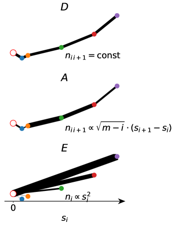
Figure 5: The $D$-, $A$-, and $E$-optimals of difference networks where the relative errors in the measurements are a constant. The width of each edge $e$ in the $\mathcal{G}_{n}$ is proportional to the allocation $n_{e}$.

In the $A$- and $D$-optimals, the subgraph of $\mathcal{G}_{n}$ consisting of only the edges with weights $n_{e}\neq 0$ is the minimum spanning tree (MST) of $\mathcal{G}_{s}$, connecting vertices $i$ and $i+1$, for $i=0,1,\dots,m-1$ (Fig. 5). The above conjectures have been corroborated by comparing the constructive solutions with the results of numerical minimizations for many sets of randomly generated $\{s_{e}\}$, but their rigorous proofs have so far defied me.

Appendix G Iterative optimization of the difference network

Better estimates of $\{s_{e}\}$ are obtained as measurements proceed, which can be used to derive improved allocations $\{n_{e}\}$. Such a measurement-allocation cycle can be iterated so that the resulting allocations in the difference network approach the true optimal.

Let $\{n_{e}\}$ be the resources already spent to perform the measurements, and $\{s_{e}\}$ be the current estimates of the fluctuations. A total of $\Delta N$ new resources are to be allocated to the measurements in the next iteration. It is straigthforward to optimize the objective functions (e.g. $\mathrm{tr}(\mathbf{C})$ in the $A$-optimal) with respect to $\{\Delta n_{e}\}$, where $\Delta n_{e}$ is the additional resource to be allocated to measurement $e$, under the constraints

$$\Delta n_{e}\geq 0\text{ for all }e\text{, and }\sum_{e}\Delta n_{e}=\Delta N.$$ (48)

For $A$-optimal, this minimization can again be cast as an SDP, replacing $\mathbf{F}(\{n_{e}\})$ in Eq. 24 with $\mathbf{F}(\{n_{e}+\Delta n_{e}\})$.

Appendix H Sparse difference network

The following outlines a heuristic approach to designing a sparse, near-optimal difference network, which is $k$-edge-connected and entails $M$ measurements, i.e. $|\mathrm{edges}(\mathcal{G}_{n})|=M$, where $|\mathrm{edges}(\mathcal{G}_{n})|$ is the number of edges with $n_{e}>0$ in the difference network $\mathcal{G}_{n}$.

1. Find the $k$-edge-connected spanning subgraph $\mathcal{G}_{k}$ of $\mathcal{G}_{s}$, such that the set of selected edges $E=\mathrm{edges}(\mathcal{G}_{k})$ minimizes $\sum_{e\in E}s_{e}$. For $k\leq 2$, this problem can be solved in polynomial time; for $k>2$, an approximate solution can be found in polynomial time Czumaj and Lingas (1999).

2. Augment $\mathcal{G}_{k}$ with $M-|\mathrm{edges}(\mathcal{G}_{k})|$ edges in $\mathrm{edges}(\mathcal{G}_{s})\setminus\mathrm{edges}(\mathcal{G}_{k})$ with the smallest $s_{e}$ values, where $\mathrm{edges}(\mathcal{G}_{s})\setminus\mathrm{edges}(\mathcal{G}_{k})$ denotes the set of edges that are in $\mathcal{G}_{s}$ but not in $\mathcal{G}_{k}$. The resulting graph $\mathcal{G}_{k,M}$ has $M$ edges and is $k$-edge-connected.

3. Setting $n_{e}=0$ for $e\not\in\mathrm{edges}(\mathcal{G}_{k,M})$, optimize the objective function with respect to $\{n_{e}|e\in\mathrm{edges}(\mathcal{G}_{k,M})\}$.

References

- Stephen Boyd (2004) Stephen Boyd, L. V. Convex optimization; Cambridge University Press, 2004, Chapter 7.
- Pukelsheim (2006) Pukelsheim, F. Optimal design of experiments; Classics in Applied Mathematics; SIAM, 2006, Vol. 50.
- Harder et al. (2016) Harder, E. et al. OPLS3: A Force Field Providing Broad Coverage of Drug-like Small Molecules and Proteins. J. Chem. Theory Comput. 2016, 12, 281–296.
- Wang et al. (2015) Wang, L. et al. Accurate and Reliable Prediction of Relative Ligand Binding Potency in Prospective Drug Discovery by Way of a Modern Free-Energy Calculation Protocol and Force Field. J. Am. Chem. Soc. 2015, 137, 2695–2703.
- Boresch et al. (2003) Boresch, S., Tettinger, F., Leitgeb, M., and Karplus, M. Absolute Binding Free Energies: A Quantitative Approach for Their Calculation. J. Phys. Chem. B 2003, 107, 9535–9551.
- Mobley et al. (2007) Mobley, D. L., Graves, A. P., Chodera, J. D., McReynolds, A. C., Shoichet, B. K., and Dill, K. A. Predicting Absolute Ligand Binding Free Energies to a Simple Model Site. J. Mol. Biol. 2007, 371, 1118–1134.
- Woo and Roux (2005) Woo, H.-J., and Roux, B. Calculation of absolute protein–ligand binding free energy from computer simulations. Proc. Natl. Acad. Sci. U.S.A. 2005, 102, 6825–6830.
- Aldeghi et al. (2015) Aldeghi, M., Heifetz, A., Bodkin, M. J., Knapp, S., and Biggin, P. C. Accurate calculation of the absolute free energy of binding for drug molecules. Chem. Sci. 2015, 7, 207–218.
- Cournia et al. (2017) Cournia, Z., Allen, B., and Sherman, W. Relative Binding Free Energy Calculations in Drug Discovery: Recent Advances and Practical Considerations. J. Chem. Inf. Model. 2017, 57, 2911-2937
- Tembre and Cammon (1984) Tembre, B. L., and Cammon, J. M. Ligand-receptor interactions. Comput. Chem. 1984, 8, 281–283.
- Radmer and Kollman (1997) Radmer, R. J., and Kollman, P. A. Free energy calculation methods: A theoretical and empirical comparison of numerical errors and a new method qualitative estimates of free energy changes. J. Comput. Chem. 1997, 18, 902–919.
- Bennett (1976) Bennett, C. H. Efficient estimation of free energy differences from Monte Carlo data. J. Comput. Phys. 1976, 22, 245–268.
- Shirts and Chodera (2008) Shirts, M. R., and Chodera, J. D. Statistically optimal analysis of samples from multiple equilibrium states. J. Chem. Phys. 2008, 129, 124105.
- Shenfeld et al. (2009) Shenfeld, D. K., Xu, H., Eastwood, M. P., Dror, R. O., and Shaw, D. E. Minimizing thermodynamic length to select intermediate states for free-energy calculations and replica-exchange simulations. Phys. Rev. E 2009, 80, 046705.
- Liu et al. (2013) Liu, S., Wu, Y., Lin, T., Abel, R., Redmann, J. P., Summa, C. M., Jaber, V. R., Lim, N. M., and Mobley, D. L. Lead optimization mapper: automating free energy calculations for lead optimization. J. Comput. Aid. Mol. Des. 2013, 27, 755–70.
- Wang et al. (2013) Wang, L., Deng, Y., Knight, J. L., Wu, Y., Kim, B., Sherman, W., Shelley, J. C., Lin, T., and Abel, R. Modeling Local Structural Rearrangements Using FEP/REST: Application to Relative Binding Affinity Predictions of CDK2 Inhibitors. J. Chem. Theory Comput. 2013, 9, 1282–93.
- Kurt Mehlhorn (2008) Kurt Mehlhorn, P. S. Algorithms and Data Structures; Springer, Berlin, Heidelberg, 2008, Chapter 10.
- (18) Andersen, M., Dahl, J., and Vandenberghe, L. CVXOPT. www.cvxopt.org.
- Yamakawa et al. (2014) Yamakawa, N., Suzuki, K., Yamashita, Y., Katsu, T., Hanaya, K., Shoji, M., Sugai, T., and Mizushima, T. Structure-activity relationship of celecoxib and rofecoxib for the membrane permeabilizing activity. Bioorg. Med. Chem. 2014, 22, 2529–2534.
- Yang et al. (2019) Yang, Q., Burchett, W. W., Steeno, G. S., Mobley, D. L., and Hou, X. Optimal Designs of Pairwise Calculation: an Application to Free Energy Perturbation in Minimizing Prediction Variability. 2019, http://dx.doi.org/10.26434/chemrxiv.7965140.v1
- Mobley and Guthrie (2014) Mobley, D. L., and Guthrie, J. P. FreeSolv: a database of experimental and calculated hydration free energies, with input files. J. Comput. Aid. Mol. Des. 2014, 28, 711–720.
- Czumaj and Lingas (1999) Czumaj, A., and Lingas, A. On Approximability of the Minimum-cost K-connected Spanning Subgraph Problem. Proceedings of the Tenth Annual ACM-SIAM Symposium on Discrete Algorithms. Philadelphia, PA, USA, 1999, pp 281–290.