Enhanced tensor non-Gaussianities in presence of a source

Abstract

We address the possibility of having an enhanced signal for tensor non-Gaussianities in presence of a source, as a signature of Primordial Gravitational Waves. We employ a nearly model-independent framework based on Effective Field Theory of inflation and compute tensor non-Gaussianities therefrom sourced by particle production during (p)reheating to arrive at an enhanced signal strength. We obtain the non-linearity parameters and also find that squeezed limit bispectra are more enhanced than equilateral limit.

1 Introduction

Even after the profound advancement in the Cosmic Microwave Background (CMB) observations for nearly two decades, Primordial Gravitational Waves (PGW) the so-called tensor modes of perturbations still remain as the holy grail of early universe cosmology. The latest bound on the amplitude of two-point correlation function of tensor modes i.e tensor-to-scalar ratio is $r<0.064$ from Planck 2018 data Akrami:2018odb . All it gives us is an impression that the signal strength of power spectrum for PGW, if exists, would be really tiny, making it a daunting task for next-generation CMB missions to detect it some day. Despite this, from theoretical point of view, PGW encodes crucial information about early universe cosmology. PGW generated due to vacuum fluctuations during inflation is directly related to inflationary energy scale. In absence of any conclusive evidence of two-point function for PGW until now, the community got curious about the three-point function that reflects the non-Gaussian features of PGW, primarily because it has potential to serve as an additional probe of PGW. Over the last few years there has been some theoretical progress in this direction. In mald1 ; mald2 the three-point function for tensor modes is calculated for general single field slow roll inflationary models. This analysis is further generalized in yamaguchi ; Naskar:2018rmu . For a recent review the reader can refer to Shiraishi:2019yux . These analysis are for tensor modes generated by vacuum fluctuations. However, it has been pointed out in a previous article by the present authors Naskar:2018rmu in a model-independent framework based on EFT of inflation, and also by others following particular models, that the amplitude of bispectrum generated by vacuum fluctuations is generically small.

Apart from vacuum fluctuations, PGW can also be generated by some sources that may be present during the early epoch. While some of these sources can affect the powerspectrum of PGW non-trivially, one can also investigate for non-Gaussian features of PGW which has different momentum dependence for different sources and hence can distinguish among different sources and vacuum. Of late this revelation has served as a strong motivation to explore non-Gaussian statistics of PGW from possible sources. Subsequently, the possibilities of producing comparatively large signal using different sources have been investigated to some extent, for example, using axion as a source Namba:2015gja ; aniket , or using extra spin particles during inflation Dimastrogiovanni:2018gkl .

The current observations are unable to detect any significant signal of tensor non-Gaussianities. Latest constraints on the amplitude of three-point function with $1\sigma$ error are $f_{NL}^{T}=600\pm 1500$ from WMAP Shiraishi:2014ila and $f_{NL}^{T}=800\pm 1100$ from Planck 2018 Akrami:2019izv for equilateral momentum configuration and on the amplitude for tensor-scalar-scalar three point function are $f_{NL}^{TSS}=84\pm 49$ at $68\%$C.L. Shiraishi:2017yrq . Nonetheless, the methodology for bispectrum estimation is established by adding B-mode polarization information Shiraishi:2019yux . Upcoming CMB mission LiteBIRD Matsumura:2013aja ; Suzuki:2018cuy targets to improve the results by three orders of magnitude. CMB-S4 Abazajian:2016yjj may improve the tensor-scalar-scalar cross correlation result by an order of magnitude. The dedicated gravitational waves detector LISA Bartolo:2018qqn can directly probe the bispectrum of gravitational waves. Future missions like Advanced LIGO TheLIGOScientific:2014jea , BBO Crowder:2005nr will work with improved sensitivity towards the detection of tensor non-Gaussianity. So it is important to do a theoretical analysis on generic aspects of tensor non-Gaussian statistics and interpret the constraints in the light of upcoming observations.

In this article we intend to take up our previous model-independent analysis Naskar:2018rmu based on EFT of inflation and extend it to possible sources. We want to explore if it is possible to enhance the bispectrum of PGW due to (p)reheating process. To this end we will make use of the EFT of inflation crem2 and EFT of (p)reheating Giblin:2017qjp . As in the case of our previous analysis Naskar:2018rmu , the present analysis depends solely on the EFT parameters and different choice of these parameters leads to different models. In particular, we would be interested in proposing expressions for non-linearity parameter $f_{NL}$ from the model independent framework of EFT.

2 EFT, Graviton Lagrangian and (P)reheating

As mentioned, since our intention is to analyze the scenario in a more or less model independent framework, we make use of the EFT of inflation following our previous analysis Naskar:2018rmu , that was originally developed in crem2 ; weinberg . In this approach, the inflaton field $\phi$ is a scalar under all diffeomorphisms but $\delta\phi$ breaks the time diffeomorphism. Using this symmetry of the system and unitary gauge where $\delta\phi=0$, the Lagrangian can be written as crem2

$$\mathcal{S}=\int d^{4}x\sqrt{-g}\left[\frac{1}{2}M_{pl}^{2}R-\Lambda(t)-c(t)g^{00}\right.\\ \left.+\frac{1}{2}M_{2}(t)^{4}(g^{00}+1)^{2}-\frac{\bar{M}_{1}(t)^{3}}{2}(g^{00}+1)\delta K_{\mu}^{\mu}\right.\\ \left.-\frac{\bar{M}_{2}(t)^{2}}{2}\delta K_{\mu}^{\mu 2}-\frac{\bar{M}_{3}(t)^{2}}{2}\delta K_{\mu}^{\nu}\delta K_{\nu}^{\mu}+\frac{M_{3}(t)^{4}}{3!}(g^{00}+1)^{3}\right.\\ \left.-\frac{\bar{M}_{4}(t)^{3}}{3!}(g^{00}+1)^{2}\delta K_{\mu}^{\mu}-\frac{\bar{M}_{5}(t)^{2}}{3!}(g^{00}+1)\delta K_{\mu}^{\mu 2}\right.\\ \left.-\frac{\bar{M}_{6}(t)^{2}}{3!}(g^{00}+1)\delta K_{\mu}^{\nu}\delta K_{\nu}^{\mu}-\frac{\bar{M}_{7}(t)}{3!}\delta K_{\mu}^{\mu 3}\right.\\ \left.-\frac{\bar{M}_{8}(t)}{3!}\delta K_{\mu}^{\mu}\delta K_{\nu}^{\rho}\delta K_{\rho}^{\nu}-\frac{\bar{M}_{9}(t)}{3!}\delta K_{\mu}^{\nu}\delta K_{\nu}^{\rho}\delta K_{\rho}^{\mu}+....\right].$$ (1)

The dots at the end of the Lagrangian represent higher order fluctuation terms. As pointed out in crem2 , this is purely gravitational Lagrangian where $R$ is the Einstein curvature term, $g^{00}$ is the time-time component of the metric tensor, $K_{\mu}^{\nu}$ is the extrinsic curvature, $\Lambda(t)$, $c(t)$, $M_{i}$ and $\bar{M}_{i}$ are the parameters of the theory where parameters $\Lambda(t)$ and $c(t)$ can be fixed by background evolution. The parameters $M_{i}$ and $\bar{M}_{i}$ can in general be time dependent but in our analysis we consider them as constants as the time dependence of these parameters is slow roll suppressed. In (1) the scalar perturbation is not explicit but can be reintroduced using $St\ddot{u}ckleberg$ trick.

In Unitary gauge the perturbed metric can be written as, $g_{ij}(t,x)=a^{2}(t)[(1+2\zeta(t,x))\delta_{ij}+\gamma_{ij}(t,x)]$, where $a(t)$ is scale factor, $\zeta(t,x)$ is scalar perturbation and $\gamma_{ij}(t,x)$ is tensor perturbation which is transverse and traceless satisfying, $\gamma_{ii}=0$ and $\partial_{j}\gamma_{ij}=0$. In terms of $\gamma_{ij}$ the Lagrangian (1) takes the form

$$S_{3}^{T}=\int d^{4}x\sqrt{-g}\left[\frac{M_{pl}^{2}}{8}\left(\dot{\gamma}_{ij}^{2}-\frac{(\partial_{k}\gamma_{ij})^{2}}{a^{2}}\right)-\frac{\bar{M}_{3}^{2}}{8}\dot{\gamma}_{ij}^{2}\right.\\ \left.-\frac{M_{pl}^{2}}{8}\left(2\gamma_{ik}\gamma_{jl}-\gamma_{ij}\gamma_{kl}\right)\frac{\partial_{k}\partial_{l}\gamma_{ij}}{a^{2}}-\frac{\bar{M}_{9}}{3!}\dot{\gamma}_{ij}\dot{\gamma}_{jk}\dot{\gamma}_{ki}\right],$$ (2)

where a dot on the operators denotes derivative with respect to time. The propagation speed of tensor fluctuation gets modified as $c_{\gamma}^{2}=\frac{M_{pl}^{2}}{M_{pl}^{2}-\bar{M}_{3}^{2}}$ due to the presence of $\bar{M_{3}}$ parameter.

Eq (2) is the most general third order Lagrangian for single field inflation. It has been shown that the term proportional to $\bar{M_{9}}$ along with the Einstein term contribute to tensor bispectrum Naskar:2018rmu . For our present investigation, our intention is to add, on top of this, the EFT of (p)reheating that was developed in Giblin:2017qjp . Here, apart from the inflaton fluctuation, one more degree of freedom is considered. This approach also assumes that the background breaks the time diffeomorphism spontaneously and the construction of the Lagrangian is similar as crem2 . For (p)reheat field $\chi$ it can be written as,

$$\mathcal{S}_{\chi}=\int d^{4}x\sqrt{-g}\left[-\frac{\alpha_{1}(t)}{2}g^{\mu\nu}\partial_{\mu}\chi\partial_{\nu}\chi+\frac{\alpha_{2}(t)}{2}(\partial^{0}\chi)^{2}\right.\\ \left.-\frac{\alpha_{3}(t)}{2}\chi^{2}+\alpha_{4}\chi\partial^{0}\chi\right].$$ (3)

Here $\alpha_{i}$’s are parameters of the theory. With time repara metrization invariance, parameter $\alpha_{4}$ has been set to zero Giblin:2017qjp . Note that the (p)reheat particles also have non-trivial propagation speed

$$c_{\chi}^{2}=\frac{\alpha_{1}}{\alpha_{1}+\alpha_{2}}.$$ (4)

In our analysis we consider $\alpha_{1}$ and $\alpha_{2}$ to be time independent and hence the propagation speed is also time independent.

3 Two-point correlation function

With (p)reheating particles as source with energy-momen tum tensor $T_{ab}(x,t)$ the equation of motion for $\gamma_{ij}(x,t)$ is given by,

$$\gamma_{ij}^{{}^{\prime\prime}}(x,\tau)-2\frac{a^{\prime}}{a}\gamma_{ij}^{\prime}(x,\tau)+c_{\gamma}^{2}\Delta\gamma_{ij}(x,\tau)=\frac{2}{M_{p}^{2}}\Pi_{ij}^{ab}T_{ab}(x,\tau).$$ (5)

Here ^′ denotes derivative with respect to conformal time $\tau$, and $\Pi_{ij}^{ab}$ is the transverse traceless projection tensor. Written explicitly,

$$\Pi_{ij}^{ab}=\Pi_{i}^{a}\Pi_{j}^{b}-\frac{1}{2}\Pi_{ij}\Pi^{ab},~{}~{}{\rm with}~{}~{}\Pi_{ij}=\delta_{ij}-\frac{\partial_{i}\partial_{j}}{\Delta}.$$ (6)

So the transverse traceless part of energy momentum tensor becomes

$$\Pi_{ij}^{ab}T_{ab}=-\alpha_{1}\Pi_{ij}^{ab}\partial_{a}\chi\partial_{b}\chi.$$ (7)

Taking Fourier transform the solution for Eq (5) can be obtained by Green’s function method,

$$\gamma_{ij}(k,\tau)=\frac{2}{M_{p}^{2}}\int d\tau^{\prime}G_{k}(\tau,\tau^{\prime})\Pi_{ij}^{ab}T_{ab}(k,\tau^{\prime}),$$ (8)

where the expression for Green’s function $G_{k}(\tau,\tau^{\prime})$ is given by,

$$G_{k}(\tau,\tau^{\prime})=\frac{1}{c_{\gamma}^{3}k^{3}\tau^{\prime 2}}\left[(1+c_{\gamma}^{2}k^{2}\tau\tau^{\prime})\sin c_{\gamma}k(\tau-\tau^{\prime})+\right.\\ \left.c_{\gamma}k(\tau^{\prime}-\tau)\cos c_{\gamma}k(\tau-\tau^{\prime})\right]\Theta(\tau-\tau^{\prime})].$$ (9)

It is worthwhile to mention that in (9) the non trivial propagation speed of tensor fluctuation plays a crucial role in determining the Green’s function and hence the powerspectrum. This will be obvious from the following analysis. In what follows we employ the method of Cook to calculate the two-point correlation function for our setup of nontrivial contribution from the EFT parameters.

Using this Green’s function the power spectrum for tensor modes sourced by (p)reheat field turns out to be

$$\left\langle\gamma_{ij}(k,\tau)\gamma^{ij}(k,\tau^{\prime})\right\rangle=\frac{\alpha_{1}^{2}}{2\pi^{3}M_{p}^{4}}\int\frac{d\tau^{\prime}}{a(\tau^{\prime})^{2}}G_{k}(\tau,\tau^{\prime})\\ \times\int\frac{d\tau^{\prime\prime}}{a(\tau^{\prime\prime})^{2}}G_{k}(\tau,\tau^{\prime\prime})\Pi_{ij}^{ab}(k)\Pi_{ij}^{cd}(k^{\prime})\\ \times\int d^{3}pd^{3}p^{\prime}p_{a}(k_{b}-p_{b})p_{c}^{\prime}(k_{d}^{\prime}-p_{d}^{\prime})\\ \times\left\langle\chi(p,\tau^{\prime})\chi(k-p,\tau^{\prime})\chi(p^{\prime},\tau^{\prime\prime})\chi(k^{\prime}-p^{\prime},\tau^{\prime\prime})\right\rangle.$$ (10)

In order to evaluate the correlation functions we need to analyze the dynamics of $\chi$ particles. Varying (3) with respect to $\chi$ one arrives at the following equation of parametric oscillator

$$\chi_{c}^{\prime\prime}(k,\tau)+\omega^{2}(k,\tau)\chi_{c}(k,\tau)=0,$$ (11)

where, $\chi_{c}=a\chi(\alpha_{1}+\alpha_{2})$ and the frequency of the oscillator is given by

$$\omega^{2}(k,\tau)=k^{2}c_{\chi}^{2}+a^{2}(\tau)\frac{\alpha_{3}(t)}{\alpha_{1}+\alpha_{2}}-\frac{a^{\prime\prime}}{a}.$$ (12)

This clearly shows the nontrivial modifications to the frequency that arises due to the EFT of (p)reheating.

Consequently, the solution for (11) becomes

$$\chi_{c}=\frac{1}{\sqrt{2\omega}}\left(\alpha(k,\tau)e^{-i\int^{\tau}\omega}+\beta(k,\tau)e^{i\int^{\tau}\omega}\right),$$ (13)

where $\alpha$ and $\beta$ are the Bogolyubov coefficients.

To proceed further, we need to find explicit time dependence of $\omega(k,\tau)$ i,e we need to find the functional form of $\frac{\alpha_{3}(t)}{\alpha_{1}+\alpha_{2}}$. In order to do that we have to remember that there are two important energy scales in the theory: the cosmological time $H^{-1}$, $H$ being the Hubble parameter and the time scale associated with the frequency of oscillations ($\omega_{osc}$) of inflaton at the end of inflation. This corresponds to a hierarchy of scales Giblin:2017qjp . At high energies $E>\omega_{osc}>H$ the time translation is unbroken. When $E<\omega_{osc}$ the time translation symmetry is broken as discrete symmetry and at even lower energy $E<H<\omega_{osc}$ cosmological expansion breaks time translation symmetry. As a consequence the background Hubble parameter can be written as a sum of slowly time dependent function and an oscillatory function Giblin:2017qjp ; Behbahani:2011it ,

$$H(t)=H_{sr}(t)+H_{osc}(t)P(\omega_{osc}t),$$ (14)

where, $H_{sr}(t)$ and $H_{osc}(t)$ are slowly time dependent functions and $P(\omega_{osc}t)$ is some periodic function. Now the parameters of EFT of (p)reheating can be written as a function of Hubble parameter and its derivatives Giblin:2017qjp and hence will be periodic in nature. If we expand the periodic function $\frac{\alpha_{3}(t)}{\alpha_{1}+\alpha_{2}}$ with frequency $\omega_{\alpha_{3}}$ around its minimum $t_{0}$ then it can be written as,

$$\frac{\alpha_{3}(t)}{\alpha_{1}+\alpha_{2}}\propto\omega_{\alpha_{3}}^{2}(t-t_{0})^{2}+...$$ (15)

In general the frequency $\omega_{\alpha_{3}}$ can be different than $\omega_{osc}$ and the dots represent higher order terms in the expansion. In our analysis we consider upto second order in time expansion. Physically the parameter $\alpha_{3}(t)$ describes the interaction between inflaton and $\chi$ particles. So our choice in (15) can be written in an alternative way in terms of inflaton field,

$$\frac{\alpha_{3}(t)}{\alpha_{1}+\alpha_{2}}=\frac{g^{2}}{2}(\phi-\phi_{0})^{2},$$ (16)

where, $\phi_{0}=\phi(t=t_{0})$ and considering de-sitter background and with slow roll approximation we can assume that, $\phi(t)=\dot{\phi_{0}}t$ where $\dot{\phi_{0}}$ is constant, so $t_{0}$ present in (15) can be written as, $t_{0}=\frac{\phi_{0}}{\dot{\phi_{0}}}$. The parameter choice of (16) is consistent with the background evolution and symmetry. With these parameter choices of EFT of inflation and EFT of (p)reheating we are able to analyze the production of PGW due to (p)reheating from a fairly general class of inflationary models and a class of (p)reheating models where the propagation speed of produced particle is non-trivial and the interaction between inflaton and the (p)reheating particles is described by (15) and (16).

With the parameter choice of (16), non-adiabatic condition leads to a constraint $g>>\frac{H^{2}}{\dot{\phi}_{0}}$, and with this constraint we can neglect the expansion of universe and can consider $H$ as a constant in time Cook . With these approximations the Bogolyubov coefficients turn out to be

$$\alpha(k,\tau>\tau_{0})=\sqrt{1+e^{\frac{-c_{\chi}^{2}k^{2}H^{2}\tau_{0}^{2}}{g\dot{\phi_{0}}}}}e^{i\alpha_{k}},$$ (17)

and

$$\beta(k,\tau>\tau_{0})=ie^{\frac{-c_{\chi}^{2}k^{2}H^{2}\tau_{0}^{2}}{2g\dot{\phi_{0}}}},$$ (18)

where $\alpha_{k}={\rm Arg}\left(\Gamma\left(1/2+i\frac{-c_{\chi}^{2}k^{2}H^{2}\tau_{0}^{2}}{2g\dot{\phi_{0}}}\right)\right)+\frac{-c_{\chi}^{2}k^{2}H^{2}\tau_{0}^{2}}{2g\dot{\phi_{0}}}(1-\log{\frac{-c_{\chi}^{2}k^{2}H^{2}\tau_{0}^{2}}{2g\dot{\phi_{0}}}})$.

With these initial conditions, we will now work in the non-relativistic limit as the Bogolyubov coefficients contain exponential momentum suppression, for which $\omega(|k-p|)-\omega(p)=0$ and $\omega^{2}=\frac{g^{2}\dot{\phi_{0}}^{2}}{H^{4}\tau^{2}}\left[\ln{\left(\frac{\tau_{0}}{\tau}\right)}\right]^{2}$.

Consequently, the two-point correlation function looks

$$\left\langle\gamma_{ij}(k,\tau)\gamma^{ij}(k^{\prime},\tau)\right\rangle=\frac{\alpha_{1}^{2}}{(\alpha_{1}+\alpha_{2})^{2}}\frac{\delta(k+k^{\prime})}{8\pi^{3}M_{p}^{4}}\int d^{3}p\left(p^{2}-\frac{\bf{p}.\bf{k}}{k^{2}}\right)^{2}\\ \times\int\frac{d\tau^{\prime}}{a(\tau^{\prime})^{2}}\frac{G_{K}(\tau,\tau^{\prime})}{\sqrt{\omega_{p}(\tau^{\prime})\omega_{k-p}(\tau^{\prime})}}\int\frac{d\tau^{\prime\prime}}{a(\tau^{\prime\prime})^{2}}\frac{G_{K}(\tau,\tau^{\prime\prime})}{\sqrt{\omega_{p}(\tau^{\prime\prime})\omega_{k-p}(\tau^{\prime\prime})}}\\ \times(2|\beta(p)|^{4}+2|\alpha(p)|^{2}|\beta(p)|^{2}).$$ (19)

The $\tau\rightarrow 0$ limit of the above Green’s function is given by, $G_{k}(0,\tau^{\prime})=\frac{c_{\gamma}k\tau^{\prime}\cos(c_{\gamma}k\tau^{\prime})-\sin(c_{\gamma}k\tau^{\prime})}{c_{\gamma}^{3}k^{3}\tau^{\prime 2}}$. Hence, upon performing the $p$ and $\tau$ integration we get,

$$\left\langle\gamma_{ij}(k,\tau)\gamma^{ij}(k^{\prime},\tau)\right\rangle=\frac{\delta(k+k^{\prime})}{4\pi^{5}M_{p}^{4}}\frac{H}{c_{\gamma}^{6}k^{6}c_{\chi}^{3}}\frac{(g\dot{\phi_{0}})^{3/2}}{\tau_{0}^{3}}\left(1+\frac{1}{4\sqrt{2}}\right)\\ \times\left(c_{\gamma}k\tau_{0}\cos(c_{\gamma}k\tau_{0})-\sin(c_{\gamma}k\tau_{0})\right)^{2}\left(\ln\frac{\sqrt{g\dot{\phi}_{0}}}{H}\right)^{2}.$$ (20)

The role of non-trivial propagation speed $c_{\gamma}$ and $c_{\chi}$ are now crystal-clear from (20). They can be used to tune the signal strength of the two-point function. For example, it can be enhanced in the limit $c_{\gamma}\rightarrow 0$ or $c_{\chi}\rightarrow 0$ or $c_{\gamma},c_{\chi}\rightarrow 0$. So, it is expected that they will play crucial role in determining the signal strength of three-point correlation functions as well. However, we will concentrate on this in the next section.

The total power spectrum for tensor modes reads

$$P_{T}(k)=\frac{2H^{2}}{M_{P}^{2}c_{\gamma}\pi^{2}}\left[1+\frac{H^{2}}{M_{p}^{2}\pi^{3}c_{\gamma}^{5}c_{\chi}^{3}}\frac{(g\dot{\phi}_{0})^{3/2}}{H^{3}}\left(1+\frac{1}{4\sqrt{2}}\right)\right.\\ \times\left.\frac{\left(c_{\gamma}k\tau_{0}\cos(c_{\gamma}k\tau_{0})-\sin(c_{\gamma}k\tau_{0})\right)^{2}}{k^{3}\tau_{0}^{3}}\left(\ln\frac{\sqrt{g\dot{\phi}_{0}}}{H}\right)^{2}\right].$$ (21)

It can be verified that the function $\frac{\left(c_{\gamma}k\tau_{0}\cos(c_{\gamma}k\tau_{0})-\sin(c_{\gamma}k\tau_{0})\right)^{2}}{c_{\gamma}^{3}k^{3}\tau_{0}^{3}}$ gets maximum value at $c_{\gamma}k\tau_{0}=2.46$. In order to compare with the existing results in the literature, we take the same representative values for the parameter as in Cook : $g=1$, $H=10^{13}{\rm GeV}/c^{2}$, $M_{p}=2.48\times 10^{18}{\rm GeV}/c^{2}$ and $\dot{\phi}_{0}=\sqrt{2\epsilon}HM_{p}$ where, $\epsilon=0.005$. As a result, the tensor power spectrum becomes

$$P_{T}(k)=\frac{2H^{2}}{M_{P}^{2}c_{\gamma}\pi^{2}}\left[1+6.75\times 10^{-6}\frac{1}{c_{\gamma}^{2}c_{\chi}^{3}}\right].$$ (22)

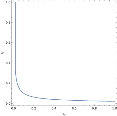
In the existing literature (e.g., Cook ), the second term in the parenthesis was generically small. However, in the present analysis, it can be significantly large due to nontrivial speed of propagation. For example, if the second term is of order of one, the signal strength of two point correlation function of PGW due to (p)reheating can be of the same order of the vacuum contribution. Fig 1 demonstrates the comparative values of the two speed of propagation in order to achieve this.

Figure 1: The correlation between $c_{\gamma}$ and $c_{\chi}$ for large contribution of reheating sourced two point correlation function

Let us explain it with a particular example. If we take a representative value for the tensor-to-scalar ratio as $r\approx 0.06$ that is close to the upper bound set by the latest Planck 2018 data Akrami:2018odb , then for $c_{\gamma}=1,~{}c_{\chi}\approx 0.02$ the second term will be $\mathcal{O}(1)$. However, the signal strength of two point correlation function due to (p)reheating particles can be much larger than the signal strength due to vacuum fluctuations if $c_{\gamma}$ and $c_{\chi}$ become smaller than the above mentioned limit. Also we have noted earlier that the signal strength gets maximum contribution for $c_{\gamma}k\tau_{0}=2.46$, so the peak frequency of the signal will be dependent on $c_{\gamma}$. The peak frequency will be higher for a smaller $c_{\gamma}$. So the detectability of the signal is dependent on the EFT parameters and as explained above there lies a region in the parameter space where the signal strength becomes strong with peak frequency determined by $c_{\gamma}$. This can be of interest for the upcoming gravitational wave (GW) missions such as the Einstein telescope Maggiore:2019uih which will operate in the high frequency limit where the GW signal strength produced from (p)reheating gets peaked.

The reason for the enhancement of the signal is that for $c_{\chi}<1$ the resonance band become broadened and there is an enhancement in particle production as discussed in Giblin:2017qjp . On the other hand according to Karouby:2011xs small propagation speed of tensor fluctuation is also responsible for large signal because non canonical inflationary case is responsible for a saw-tooth like profile of inflaton which moves the system to broad parametric resonance and significant particle production occurs. Note that in the above analysis we did not consider the non-adiabatic scenario as it is shown in Cook that this regime produces same result as the adiabatic regime.

4 Three-point correlation function

Having convinced ourselves about the role of the non-trivial propagation speed on the signal strength, let us now move forward to calculate the three-point function for (p)reheating-sourced gravitational waves. The expression for three-point function is given by

$$\langle\gamma^{s_{1}}(k_{1})\gamma^{s_{2}}(k_{2})\gamma^{s_{3}}(k_{3})\rangle=\left(\frac{-2\alpha_{1}}{2\pi^{2}M_{p}^{2}}\right)^{3}\int\frac{d\tau_{1}d\tau_{2}d\tau_{3}}{a(\tau_{1})^{2}a(\tau_{2})^{2}a(\tau_{3})^{2}}\\ \times e^{s_{1}}_{i_{1}j_{1}}e^{s_{2}}_{i_{2}j_{2}}e^{s_{3}}_{i_{3}j_{3}}\Pi_{i_{1}j_{1}}^{ab}(k_{1})\Pi_{i_{2}j_{2}}^{cd}(k_{2})\Pi_{i_{3}j_{3}}^{ef}(k_{3})p_{1a}p_{1b}p_{2c}p_{2d}p_{3e}p_{3f}\\ \times\langle\chi(p_{1},\tau_{1})\chi(k_{1}-p_{1},\tau_{1})\chi(p_{2},\tau_{2})\chi(k_{2}-p_{2},\tau_{2})\chi(p_{3},\tau_{3})\chi(k_{3}-p_{3},\tau_{3})\rangle,$$ (23)

where $s_{i}$ are helicity indices and $e^{s_{i}}_{ij}$ are polarization tensors. To fix the representation of polarization tensors we take a particular $k_{i}$ basis and consider that this basis is lying on $(x,y)$ plane. In doing so we will not lose any generality because of the momentum conserving $\delta$ function. In what follows we will choose the representation adapted in Soda:2011am : $k_{1}=k_{1}(1,0,0)$, $k_{2}=k_{2}(\cos\theta_{1},\sin\theta_{1},0)$, $k_{3}=k_{3}(\cos\theta_{2},\sin\theta_{2},0)$ where
$\cos\theta_{1}=\frac{k_{3}^{2}-k_{1}^{2}-k_{2}^{2}}{2k_{1}k_{2}}$,
$\sin\theta_{1}=\frac{\sqrt{2k_{1}^{2}k_{2}^{2}+2k_{2}^{2}k_{3}^{2}+2k_{1}^{2}k_{3}^{2}-k_{1}^{4}-k_{2}^{4}-k_{3}^{4}}}{2k_{1}k_{2}}$,
$\cos\theta_{2}=\frac{k_{2}^{2}-k_{1}^{2}-k_{3}^{2}}{2k_{1}k_{3}}$,
$\sin\theta_{2}=-\frac{\sqrt{2k_{1}^{2}k_{2}^{2}+2k_{2}^{2}k_{3}^{2}+2k_{1}^{2}k_{3}^{2}-k_{1}^{4}-k_{2}^{4}-k_{3}^{4}}}{2k_{1}k_{3}}$.

With this choice the polarization tensors can be written as,

$$e^{s_{1}}(k_{1})=\begin{pmatrix}0&0&0\\ 0&1&is_{1}\\ 0&is_{1}&-1\end{pmatrix},$$ (24)

$$e^{s_{2}}(k_{2})=\begin{pmatrix}\sin^{2}\theta_{1}&-\sin\theta_{1}\cos\theta_{1}&-is_{2}\sin\theta_{1}\\ -\sin\theta_{1}\cos\theta_{1}&\cos^{2}\theta_{1}&is_{2}\cos\theta_{1}\\ -is_{2}\sin\theta_{1}&is_{2}\cos\theta_{1}&-1\end{pmatrix},$$ (25)

$$e^{s_{2}}(k_{3})=\begin{pmatrix}\sin^{2}\theta_{2}&-\sin\theta_{2}\cos\theta_{2}&-is_{2}\sin\theta_{2}\\ -\sin\theta_{2}\cos\theta_{2}&\cos^{2}\theta_{2}&is_{2}\cos\theta_{2}\\ -is_{2}\sin\theta_{2}&is_{2}\cos\theta_{2}&-1\end{pmatrix}.$$ (26)

Consequently, the total three-point function gives us,

$$\langle\gamma^{s_{1}}(k_{1})\gamma^{s_{2}}(k_{2})\gamma^{s_{3}}(k_{3})\rangle_{\rm total}=\langle\gamma^{s_{1}}(k_{1})\gamma^{s_{2}}(k_{2})\gamma^{s_{3}}(k_{3})\rangle_{\rm vac}\\ +\langle\gamma^{s_{1}}(k_{1})\gamma^{s_{2}}(k_{2})\gamma^{s_{3}}(k_{3})\rangle_{\rm so},$$ (27)

where the subscripts ”vac” and ”so” stand for ”vacuum” and ”source” (here, (p)reheating) respectively and these abbreviations would be used in the rest of the article.

As already mentioned, the vacuum solution has been explored at length in a previous article by the present authors Naskar:2018rmu and is given as,

$$\langle\gamma^{s_{1}}(k_{1})\gamma^{s_{2}}(k_{2})\gamma^{s_{3}}(k_{3})\rangle_{\rm vac}=(2\pi)^{3}\delta^{(3)}({k_{1}}+{k_{2}}+{k_{3}})\\ \times F(s_{1}k_{1},s_{2}k_{2},s_{3}k_{3})\\ \times\left(\frac{64H^{4}}{c_{\gamma}^{2}M_{pl}^{4}}\frac{A(k_{1},k_{2},k_{3})(s_{1}k_{1}+s_{2}k_{2}+s_{3}k_{3})^{2}}{k_{1}^{3}k_{2}^{3}k_{3}^{3}}\right.\\ \left.+\frac{4\bar{M}_{9}H^{5}}{M_{pl}^{6}}\frac{1}{k_{1}k_{2}k_{3}}\frac{1}{(k_{1}+k_{2}+k_{3})^{3}}\right),$$ (28)

where $A(k_{1},k_{2},k_{3})=\frac{K}{16}\left(1-\frac{1}{k^{3}}\sum_{i\neq j}k_{i}^{2}k_{j}-\frac{4k_{1}k_{2}k_{3}}{K^{3}}\right)$ with ${K}=k_{1}+k_{2}+k_{3}$, and $F(x,y,z)=-\frac{1}{64x^{2}y^{2}z^{2}}(x+y+z)^{3}(x+y-z)(x-y+z)(y+z-x).$

We will calculate the contribution from source term here. In evaluating the three-point function, we will use the same approximation of adiabatic regime as in the case of two-point function. By employing this approximation, the source part of the three-point function takes the form

$$\langle\gamma^{s_{1}}(k_{1})\gamma^{s_{2}}(k_{2})\gamma^{s_{3}}(k_{3})\rangle_{\rm so}=-\left(\frac{2}{(2\pi M_{p})^{2}}\right)^{3}\frac{\alpha_{1}^{3}}{(\alpha_{1}+\alpha_{2})^{3}}\\ \times\frac{H^{12}\tau_{0}^{6}}{g^{3}\dot{\phi}_{0}^{3}k_{1}^{3}k_{2}^{3}k_{3}^{3}c_{\gamma}^{9}}\left(\ln\frac{\sqrt{g\dot{\phi}_{0}}}{H}\right)^{3}(\mathcal{A}_{k}+\mathcal{B}_{k})\\ \times\prod_{i=1}^{3}\left(c_{\gamma}k_{i}\tau_{0}\cos(c_{\gamma}k_{i}\tau_{0})-\sin(c_{\gamma}k_{i}\tau_{0})\right),$$ (29)

where the terms $\mathcal{A}_{k}$ and $\mathcal{B}_{k}$ have very tedious expressions. For completeness, we summaries them below:

$$\mathcal{A}_{k}=\frac{(g\dot{\phi}_{0})^{\frac{7}{2}}}{124416c_{\chi}^{9}H^{9}\pi^{3}\tau_{0}^{9}}\frac{\left(k_{1}^{4}+(k_{2}^{2}-k_{3}^{2})^{2}-2k_{1}^{2}(k_{2}^{2}+k_{3}^{2})\right)}{k_{1}^{2}k_{2}^{2}k_{3}^{2}}\\ \times\left(-3(81\sqrt{2}+16\sqrt{3})\right)\pi\tau_{0}^{2}H^{2}c_{\chi}^{2}\\ \times\left\{k_{1}^{4}+k_{1}^{2}(6k_{2}^{2}-2k_{3}^{2})+(k_{2}^{2}-k_{3}^{2})^{2}+4k_{1}^{3}k_{2}s_{1}s_{2}\right.\\ \left.+4k_{1}k_{2}(k_{2}^{2}-k_{3}^{2})^{2}s_{1}s_{2}\right\}+5~{}perms,$$ (30)

$$\mathcal{B}_{k}=\frac{(g\dot{\phi}_{0})^{\frac{7}{2}}}{124416c_{\chi}^{9}H^{9}\pi^{3}\tau_{0}^{9}}\frac{\left(k_{1}^{4}+(k_{2}^{2}-k_{3}^{2})^{2}-2k_{1}^{2}(k_{2}^{2}+k_{3}^{2})\right)}{k_{1}^{2}k_{2}^{2}k_{3}^{2}}g\dot{\phi}\\ \times 2(243\sqrt{2}+32\sqrt{3})(k_{1}^{2}+k_{2}^{2}+k_{3}^{2}+2(2k_{1}k_{2}s_{1}s_{2}+2k_{1}k_{3}s_{1}s_{3}+2k_{2}k_{3}s_{2}s_{3})).$$ (31)

Note that $\mathcal{B}_{k}$ is the sum of all six permutations.

As mentioned, the resulting three-point function (27) is the sumtotal of (28) and (29).

Let us now critically investigate for the results thus obtained. To do so, we will have the following observations. First, from the expression of $\mathcal{A}_{k}$ and $\mathcal{B}_{k}$ we can see that they can be written as,

$$\mathcal{A}_{k}=C(c_{\chi}^{2}f(k)),$$ (32)

$$\mathcal{B}_{k}=C(g\dot{\phi}g(k)).$$ (33)

Where $C=\frac{1}{124416c_{\chi}^{8}H^{8}\pi^{3}\tau_{0}^{8}}\sqrt{\frac{g\dot{\phi}}{c_{\chi}^{2}H^{2}\tau_{0}^{2}}}(g\dot{\phi})^{3}$ and $f(k)$ and $g(k)$ encodes all the momentum dependence and relevant prefactors. It is evident from the above expression that for a small $c_{\chi}$ we can neglect $\mathcal{A}_{k}$ and only $\mathcal{B}_{k}$ contributes to the three point function. Secondly, the term $\left(c_{\gamma}k_{i}\tau_{0}\cos(c_{\gamma}k_{i}\tau_{0})-\sin(c_{\gamma}k_{i}\tau_{0})\right)$ can be expanded for small $c_{\gamma}$ and upto third order in $c_{\gamma}$ can be written as, $(c_{\gamma}k_{i}\tau_{0})^{3}$. In order to extract out the momentum dependence of the bispectra from complicated functional form of $\mathcal{B}_{k}$ we are working in a limit where we can keep up to $c_{\gamma}^{3}$ term and can neglect $c_{\chi}^{2}$ term.

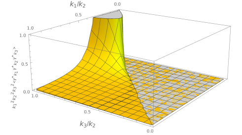
Figure 2: The bispectra is plotted as a function of $\frac{k_{1}}{k_{2}}$ and $\frac{k_{3}}{k_{2}}$

The resultant contributions have been pictorially depicted in Fig 2. The figure shows the momentum dependence of the bispectra as a function of $\frac{k_{1}}{k_{2}}$ and $\frac{k_{3}}{k_{2}}$. The essential conclusion that can be readily obtained from the above figure is that for $\frac{k_{1}}{k_{2}}\rightarrow 0$ and $0.755<\frac{k_{3}}{k_{2}}\leq 1$ we get large amplitude for the bispectra. This shows that intermediate momentum configurations other than squeezed limit and equilateral limit can contribute significantly to the signal. Also we get positive contribution for squeezed and equilateral limit and much larger amplitude for the bispectra which cannot be achieved in case of vacuum. This was the primary goal of the present article. We shall elaborate more on this in the following section.

5 Estimation of $f_{NL}$

We are now in a position to calculate the expressions for the nonlinearity parameter $f_{NL}$. In what follows we shall make use of the same definition of the non-linearity parameter as adopted in Naskar:2018rmu , namely, $\frac{6}{5}f_{NL}=\frac{\langle\gamma\gamma\gamma\rangle}{P_{\zeta}(k_{1})+P_{\zeta}(k_{2})+P_{\zeta}(k_{3})}$, where $P_{\zeta}(k)$ is the scalar powerspectrum and can be written as,
$P_{\zeta}(k)=\frac{2\pi}{k^{3}}\frac{H^{2}}{8\pi M_{pl}^{2}c_{s}}\left(\frac{k}{k_{*}}\right)^{(n_{s}-1)}$ with $n_{s}$ and $c_{s}$ being the spectral tilt and sound speed of scalar perturbations respectively. Also, the tensor modes generated due to vacuum fluctuation would in any case be small, the templates for which have already been proposed in the previous article Naskar:2018rmu . Hence, in this article we would be interested only about the three-point function due to source term $\langle\gamma^{s_{1}}(k_{1})\gamma^{s_{2}}(k_{2})\gamma^{s_{3}}(k_{3})\rangle_{\rm so}$ in formulating the templates. As has been pointed out, we are interested about any significant enhancement of signal. Hence, we would consider the scenario where the three-point function due to source term would have been dominant contribution to $\langle\gamma^{s_{1}}(k_{1})\gamma^{s_{2}}(k_{2})\gamma^{s_{3}}(k_{3})\rangle_{\rm total}$ in Eq (27) and would investigate if this is achievable with the parameters under consideration.

Like the vacuum solution, in the case of equilateral limit $k_{1}=k_{2}=k_{3}$ we have two independent non-linearity parameters. They are given by

$$f_{NL}^{+++,eq}=f_{NL}^{---,eq}=\frac{1945.07g\dot{\phi}_{0}\left(\ln\frac{\sqrt{g\dot{\phi}_{0}}}{H}\right)^{3}}{M_{p}^{2}c_{\gamma}^{7}c_{\chi}^{3}k_{1}^{3}\tau_{0}^{3}}\\ \times\left(c_{\gamma}k_{1}\tau_{0}\cos(c_{\gamma}k_{1}\tau_{0})-\sin(c_{\gamma}k_{1}\tau_{0})\right)^{3}\\ \times\left(\frac{c_{s}\epsilon}{c_{\gamma}}\right)^{2}\frac{\sqrt{g\dot{\phi}_{0}}}{H}\left(k_{1}/k_{*}\right)^{-2(n_{s}-1)},$$ (34)

$$f_{NL}^{+-+,eq}=f_{NL}^{++-,eq}=f_{Nl}^{-+-,eq}\\ =f_{NL}^{--+,eq}=f_{NL}^{+--,eq}=f_{NL}^{-++,eq}=\\ \frac{216.12g\dot{\phi}_{0}\left(\ln\frac{\sqrt{g\dot{\phi}_{0}}}{H}\right)^{3}(c_{\gamma}k_{1}\tau_{0}\cos(c_{\gamma}k_{1}\tau_{0})-\sin(c_{\gamma}k_{1}\tau_{0}))^{3}}{M_{p}^{2}c_{\gamma}^{7}c_{\chi}^{3}k_{1}^{3}\tau_{0}^{3}}\\ \times\left(\frac{c_{s}\epsilon}{c_{\gamma}}\right)^{2}\frac{\sqrt{g\dot{\phi}_{0}}}{H}\left(k_{1}/k_{*}\right)^{-2(n_{s}-1)}.$$ (35)

Consequently, for the squeezed limit, we get the following non-linearity parameters

$$f_{NL}^{+++,sq}=f_{NL}^{---,sq}=f_{NL}^{+--,sq}=f_{NL}^{-++,sq}\underset{k_{1}\rightarrow 0}{=}\\ \frac{3457.89g\dot{\phi}\left(\ln\frac{\sqrt{g\dot{\phi}}}{H}\right)^{3}}{M_{p}^{2}c_{\gamma}^{7}c_{\chi}^{3}k_{2}^{3}\tau_{0}^{3}}\prod_{i=1}^{3}\left(c_{\gamma}k_{i}\tau_{0}\cos(c_{\gamma}k_{i}\tau_{0})-\sin(c_{\gamma}k_{i}\tau_{0})\right)\\ \times\left(\frac{c_{s}\epsilon}{c_{\gamma}}\right)^{2}\frac{\sqrt{g\dot{\phi}}}{H}\left(k_{2}/k_{*}\right)^{-2(n_{s}-1)}.$$ (36)

We can see from the above expressions of $f_{NL}$ that a small propagation speed of either tensor fluctuations or preheating particles can lead to a large amplitude for tensor bispectrum. The non-Gaussian signal produced from (p)reheating can not be observed in CMB scales but can be observable in GW interferometers. However current interferometers still do not probe the scales where the signal can be detectable. But we should note that as the signal can be large for parameter combination mentioned above, the next iterations of the interferometers which can probe higher frequencies can have a chance to detect them.

Here we consider CMB constraints on squeezed limit and equilateral limit bispectra Shiraishi:2019yux ; Shiraishi:2013wua ; Ade to show the difference in magnitude of equilateral and squeezed limit and to demonstrate how the constraint on $c_{\chi}$ changes, though one should remember that CMB constraint may not be applicable to the derived $f_{NL}$. As we have stated earlier, from (p)reheating the two point function is peaked at $c_{\gamma}k_{i}\tau_{0}=2.46$ and for $c_{\gamma}=1$ and $c_{\chi}=0.02$ the signal strength becomes of the same order of vacuum contribution. For squeezed limit $f_{NL}$ where one momentum is smaller than the other two momenta, we consider that $\frac{k_{\rm large}}{k_{\rm small}}\approx 10$. The constraint on squeezed limit from Planck is $290\pm 180$ Ade . Using the above approximations and the upper limit of observational value of $f_{NL}^{+++,sq}=470$ we get $c_{\chi}>0.2$. Using the new constraint on $c_{\chi}$ we can estimate the $f_{NL}^{+++,eq}=0.3\left(k_{1}/k_{*}\right)^{0.071}$. Here we have used the best fit value for $n_{s}=0.9645$ from Planck 2018 Akrami:2018odb . From these estimations we can see that for $c_{\gamma}=1$ and small $c_{\chi}$ squeezed limit bispectrum is much larger than equilateral limit for PGW produced from (p)reheating. This nature is also visible in Fig 2, but there we used an approximation such that we can keep terms upto $c_{\chi}^{3}$ and neglect terms proportional to $c_{\chi}$. So for small $c_{\chi}$ squeezed limit will always be larger than the equilateral limit independent of whether $c_{\gamma}$ is small or unity.

Of course, these numerical estimations are not too accurate as we have considered the coupling constant to be $\mathcal{O}(1)$ which may not be strictly valid. Also one have to use the late time GW detectors’ constraint on $f_{NL}$ to analyze the scenario. In this work we refrain from commenting about the detectability of the signal by upcoming GW missions rather our target was to demonstrate that using EFT in inflation and (p)reheating, large signal for tenor non-Gaussianities can be produced due to the presence of non trivial propagation speed of $\chi$ particles and tensor modes.

The bottomline of the above analysis is that we can have an enhanced tensor non-Gaussian signal from (p)reheating with non-trivial propagation speed $c_{\chi}$. Also, particle production from non-canonical inflation with $c_{\gamma}<1$ can enhance the tensor non-Gaussian signal further. A rather conservative statement would be that, the non-Gaussian signal produced from (p)reheating can fall well within the reach of next generation GW missions. As mentioned earlier Einstein telescope will operate on the relevant frequency range to detect preheating produced GW signal Maggiore:2019uih , and this non-trivial non-Gaussian property of PGW can be of relevance for this kind of observations. However, an actual comparison with the sensitivity of upcoming GW missions can only confirm this.

6 Conclusion

In this article we have presented a way to enhance the signal for tensor three-point function sourced by (p)reheating. Our analysis is based on EFT of inflation and (p)reheating, so we were able to analyze a large class of models where the interaction between inflaton and (p)reheating particle is described by the choice of the EFT parameter $\alpha_{3}$. Using EFT we have been able to deal with a non standard case for (p)reheating for which the propagation speed of (p)reheat particle $\chi$ is different from unity. We have demonstrated that tuning this non-trivial propagation speed of (p)reheating particles along with the propagation speed of tensor fluctuation one can actually enhance the signal of tensor non-Gaussianities which was not achievable in the vacuum as well as in the standard (p)reheating analysis. We have further been able to propose templates for the non-linearity parameter $f_{NL}$ for these class of models and found that, like the source-free case, here also squeezed limit bispectrum is stronger than equilateral limit. As a result, possibility of detection in future mission of the squeezed limit is higher along with the momentum range described in Section IV. An actual comparison with the sensitivity of upcoming GW missions is beyond the scope of present article. We hope to address this issue with forecasts on couple of next-generation surveys in near future.