Chemical Compositions of Field and Globular Cluster RR Lyrae Stars: II. $\omega$ Centauri

Abstract

We present a detailed spectroscopic analysis of RR Lyrae (RRL) variables in the globular cluster NGC 5139 ($\omega$ Cen). We collected optical (4580–5330 Å), high resolution ($R\sim$ 34,000), high signal-to-noise ratio ($\sim$200) spectra for 113 RRLs with the multi-fiber spectrograph M2FS at the Magellan/Clay Telescope at Las Campanas Observatory. We also analysed high resolution ($R\sim$ 26,000) spectra for 122 RRLs collected with FLAMES/GIRAFFE at the VLT, available in the ESO archive. The current sample doubles the literature abundances of cluster and field RRLs in the Milky Way based on high resolution spectra. Equivalent width measurements were used to estimate atmospheric parameters, iron, and abundance ratios for $\alpha$ (Mg, Ca, Ti), iron peak (Sc, Cr, Ni, Zn), and s-process (Y) elements. We confirm that $\omega$ Cen is a complex cluster, characterised by a large spread in the iron content: $-$2.58 $\leq$ [Fe/H] $\leq$ $-$0.85. We estimated the average cluster abundance as $\langle$[Fe/H]$\rangle$ = $-$1.80 $\pm$ 0.03, with $\sigma$ = 0.33 dex. Our findings also suggest that two different RRL populations coexist in the cluster. The former is more metal-poor ([Fe/H] $\lesssim$ $-$1.5), with almost solar abundance of Y. The latter is less numerous, more metal-rich, and yttrium enhanced ([Y/Fe] $\gtrsim$ 0.4). This peculiar bimodal enrichment only shows up in the s-process element, and it is not observed among lighter elements, whose [X/Fe] ratios are typical for Galactic globular clusters.

1 Introduction

$\omega$ Cen (NGC 5139) is the most massive cluster in the Galaxy (4.05 $\times$ 10⁶ M_⊙, D’Souza & Rix, 2013), containing $\sim$1.7 $\times$ 10⁶ stars (Castellani et al., 2007). $\omega$ Cen is known to host stars that cover a broad range in metallicity, from [Fe/H] $\sim-2.5$ to [Fe/H] $\sim 0.0$ (Calamida et al., 2009; Johnson & Pilachowski, 2010; Marino et al., 2011; Pancino et al., 2011; Villanova et al., 2014). This large metallicity spread, coupled with an age spread of $\sim$2 Gyr (Villanova et al., 2014), suggests that $\omega$ Cen should be identified as the remnant core of a larger pristine dwarf galaxy, successively accreted by the Milky Way (Bekki & Freeman, 2003; Da Costa & Coleman, 2008; Marconi et al., 2014; Ibata et al., 2019). On the other hand, many studies suggest different origins, with $\omega$ Cen as the possible result of successive merging of inhomogeneous, coeval, proto-cluster clouds (Tsujimoto & Shigeyama, 2003), or the result of a self-enrichment history within the cluster itself (Cunha et al., 2002). A general consensus about this peculiar cluster has not been reached.

Despite the uncertainties about its origin, $\omega$ Cen has several advantages related to its peculiar characteristics. Its huge number of stars permits estimation of its distance with multiple techniques, such as variable stars like Miras (Feast, 1965), SX Phoenicis (McNamara, 2000), Type II Cepheids (Matsunaga et al., 2006), and RR Lyraes (Braga et al., 2018; Bono et al., 2019), the tip of the red giant branch (Bono et al., 2008), or the white dwarf cooling sequence (Calamida et al., 2008). Among them, the large population of candidate RRLs ($\sim$200 stars, Navarrete et al., 2015; Braga et al., 2018), makes $\omega$ Cen the ideal laboratory for a large investigation with multi-object spectroscopy. The multiple possibilities for a distance estimates, the large metallicity spread, and the large number of stars, provide a unique possibility to calibrate RRL period-luminosity-metallicity (PLZ) and period-Wesenheit-metallicity (PWZ) relations with a high level of accuracy, which then can be applied to other RRL samples in the Galaxy.

Photometric investigations concerning the RRLs in $\omega$ Cen date back to more than one century ago (Bailey, 1902) and they have been crucial objects for understanding the pulsation and evolutionary properties of old, low-mass helium burning variables (Martin & Plummer, 1915; Baade, 1958; Sandage, 1981a, b; Bono et al., 2001, 2003). Optical time series CCD data were collected both by OGLE (Udalski et al., 1992) and by CASE (Kaluzny et al., 2004) experiments, and more recently by Weldrake et al. (2007). More recently, a complete optical ($UBVRI$, Braga et al., 2016) and near-infrared ($JHK_{s}$, Navarrete et al., 2015; Braga et al., 2018) census have been published. As usual, the high-resolution spectroscopic investigations lag when compared to the photometric ones. Some abundance analyses have been performed on the $\omega$ Cen RRLs, based either on spectroscopic (Gratton et al., 1986, 18 stars), on spectrophotometric (Rey et al., 2000, 131 stars), or on photometric (Bono et al., 2019, 170 stars) techniques. However, the only large investigation based on high resolution spectroscopy was performed by Sollima et al. (2006, 74 stars collected at $R$ $\sim$ 22,500). This work aims at improving the sample of available high resolution spectroscopic abundances for the RRLs in $\omega$ Cen, based on the techniques already applied in (Magurno et al., 2018, hereinafter Paper I) for the smaller mono-metallic globular cluster NGC 3201.

We describe the collected dataset and the instrument settings in Section 2. Section 3 describes the analysis of radial velocities. The investigation methodology is presented in Section 4, and the abundance results are shown in Section 5 for iron, in Section 6 for the $\alpha$-elements, in Section 7 for the iron-peak elements, and in Section 8 for the yttrium. Finally, conclusions are presented in Section 9.

2 Instrument and data sample

Between 2015 February and April, we collected single epoch, high signal-to-noise ratio (S/N $\sim$ 200), high-resolution spectra of 126 stars in the globular cluster $\omega$ Cen (details in Table 1), uniformly distributed around the cluster center within a radius of about 15 arcmin from the cluster center (Figure 1). The spectra were collected with the Michigan/Magellan Fiber System (M2FS; Mateo et al. 2012) installed at the Magellan/Clay 6.5m telescope at Las Campanas Observatory in Chile. The selected spectrograph configuration limits the spectral coverage to 11 overlapping echelle orders in the range 4580–5330 Å. The 95 $\micron$ slit size allows a spectral resolution $R$ $\equiv$ $\lambda/\Delta\lambda$ $\simeq$ 34,000. Figure 2 compares a portion of the M2FS spectral range for two RRab stars with different metallicity, collected at similar pulsation phases.

The sample of RRLs to be observed was selected as follows: we started with the variable stars catalogue by Samus et al. (2009), and the two large RRL catalogues by Kaluzny et al. (2004) and (Clement et al., 2001, and following updates), restricted to those stars within the field of view of M2FS. The Clement et al. on-line database is not independent of the other two. We also have our own positions from the FourStar (Persson et al., 2013) dataset, already used in Braga et al. (2018). These have high accuracy because the pixel scale of FourStar is 0.16^′′/pixel and the typical image full width at half maximum (FWHM) for the infrared photometry is $\sim$0.5^′′ or better. We first checked the targets positions because the M2FS fibers are placed in pre-drilled holes that must be accurate. We started with a sample of all the relevant stars, weeded out the ones for which Clement et al. has doubts, used the FourStar images to delete crowded stars, and adopted the FourStar positions where appropriate. This sample contained 160 RRLs, with roughly equal numbers of RRab and RRc. The sample was divided into nine slices, each containing roughly 160/9 $\simeq$ 18 stars. Because 16 spectra were obtained per setup (i.e. slice) on the two M2FS camera/detector units, this ensured that not all the stars could be observed. A choice necessitated by observing convenience and total available telescope time. Stars in the last slice were observed in 2016, about a year after the other eight. Their spectra were of inferior quality and were not included in the analysis. This left 8 slices $\times$ 16 stars/slice = 128 spectra. Of these, two spectra were unusable leaving the final sample of 126.

Unfortunately, while the sample was being cleaned, a few radial velocity non-cluster members and light curve non-RRL stars were mistakenly included. Among the 126 collected spectra, three objects were marked as non cluster members because of their almost null radial velocity, not compatible with the cluster (see Section 3), and they were removed from the final sample. The remaining 123 spectra can be distinguished into 113 RRLs and 10 non-RRL stars. Only one RR Lyrae, V38, was observed twice. The main body of the paper only refers to the RRLs, whereas the non-RRL stars are briefly described in the Appendix.

In addition to our M2FS data, we also analysed a sample of 560 multi-epoch spectra for 122 RRLs from the ESO archive, collected with the multi-object, medium-high resolution spectrograph FLAMES/GIRAFFE (Pasquini et al., 2002). We selected from the archive all the available RRL spectra collected with the HR13 grism, covering the wavelength range 6120–6405 Å with a spectral resolution $R\simeq$ 26,400.

In total, 22 RRLs were only observed with M2FS, 31 RRLs were only observed with GIRAFFE, and 91 RRLs have spectra collected with both M2FS and GIRAFFE.

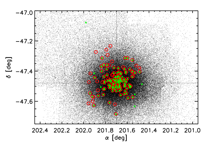
Figure 1: Radial distribution of the RRLs in our spectroscopic samples. The targets collected with M2FS and FLAMES/GIRAFFE are marked with red circles and green triangles, respectively. The cluster center is marked by the black crossing lines.

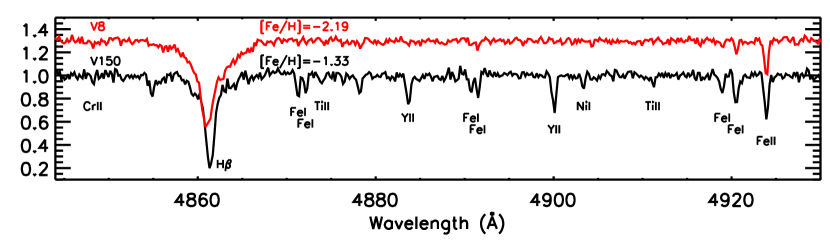
Figure 2: Comparison of a portion of the M2FS spectral range for two RRab stars, V8 and V150, observed at similar phases ($\phi\sim 0.2$). The location of some useful absorption lines are marked for iron, $\alpha$, iron peak, and s-process elements. The metal-poor spectrum (red) is vertically shifted for convenience.

Table 1: Photometric parameters and radial velocities for the sample stars in $\omega$ Cen, collected with M2FS.

ID	$\alpha$	$\delta$	period	HJD	phase	type	$\langle$V$\rangle$	$A_{V}$	$RV$
	J2000	J2000	days	2450000$+$			mag	mag	km s-1
V4	13:26:12.94	$-$47:24:19.2	0.62731846	7077.79451	1.00	RRab	14.467	1.119	202.5
V5	13:26:18.34	$-$47:23:12.8	0.51528002	7077.79451	0.59	RRab*	14.702	0.852	242.8
V7	13:27:01.04	$-$47:14:00.1	0.71303420	7086.82140	0.52	RRab	14.594	0.950	242.8
V8	13:27:48.43	$-$47:28:20.6	0.52132593	7125.83064	0.25	RRab	14.671	1.263	221.9
V10	13:26:07.01	$-$47:24:37.0	0.37475609	7077.79451	0.34	RRc	14.505	0.421	249.8
V11	13:26:30.56	$-$47:23:01.9	0.56480650	7087.78075	0.44	RRab*	14.476	0.453	243.3
V12	13:26:27.19	$-$47:24:06.6	0.38677657	7084.78661	0.58	RRc	14.498	0.438	229.3
V16	13:27:37.71	$-$47:37:35.0	0.33019610	7125.83063	0.73	RRc	14.558	0.487	228.7
V18	13:27:45.07	$-$47:24:56.9	0.62168636	7125.83064	0.87	RRab	14.551	1.152	225.8
V20	13:27:14.05	$-$47:28:06.8	0.61558779	7082.75671	0.36	RRab	14.540	1.098	232.5

3 Radial Velocities

Estimating the radial velocity ($RV$) is a common way to establish whether a star is a globular cluster member. $\omega$ Cen has had many $RV$ membership investigations thanks to its huge stellar population. Recently, An et al. (2017) estimated a cluster average velocity of 232.7 $\pm$ 0.6 km s^-1, with a dispersion $\sigma$ = 14.4 km s^-1, by using 581 red giant branch (RGB) stars. A decade earlier, Reijns et al. (2006) performed the largest investigation of $\omega$ Cen, estimating an average radial velocity of 231.3 $\pm$ 0.3 km s^-1 ($\sigma$ = 11.7 km s^-1), with 1589 RGB stars. This very large cluster $RV$ makes it unlikely that a field star in its sightline could be erroneously identified as a cluster member.

Nevertheless, we are dealing with variable stars and single epoch measurements are affected by intrinsic radial velocity variations along the pulsation cycle. Indeed, RRL pulsation cycles cause variations up to $\sim$70 km s^-1 in the observed $RV$s for RRab and up to $\sim$45 km s^-1 for RRc. Therefore, it was necessary to correct their observed radial velocities for the pulsational components, in order to determine their systemic (cluster) velocities, applying the velocity templates described in the following.

We first measured the instantaneous radial velocities using the task fxcor in IRAF (Tody, 1986, 1993). The individual spectra were cross-correlated with a synthetic spectrum generated with the driver synth of the local thermodynamic equilibrium (LTE) line analysis code MOOG (Sneden, 1973). This model spectrum was computed with the atmospheric parameters typical of stars in the RRL domain ($T_{\rm eff}$ = 6500 K, log g = 2.5, $\xi_{\rm turb}$ = 3.0 km s^-1, [Fe/H] = $-$1.5; For et al., 2011; Sneden et al., 2017) and then smoothed to the M2FS or GIRAFFE resolution. The individual velocities are listed in the last column of Table 1, and we assume an average error for the entire sample of $\sim$1.3 km s^-1, as given by fxcor.

The use of multiple $RV$ measurements allows us to improve the phasing of the individual data. The phase of the individual measurements was computed by using the period and the epoch of maximum light, relying on the work by Braga et al. (2016, 2018) for the most updated and homogeneous photometry, in the $UBVRIJHK_{s}$ bands, of the $\omega$ Cen RRLs. However, this approach is prone to possible systematics in cases of a large time interval between photometric and spectroscopic observations. Indeed, small errors in the determination of the period and/or in the epoch of maximum light could transform into large errors in the phase determination. Note that typical RRL periods range over about 6–18 hours (0.25–0.75 d). Moreover, for RRLs that are located in the cluster outskirts, we still lack accurate epoch of maximum light (Navarrete et al., 2015; Braga et al., 2018). On the other hand, radial velocities are measured with high precision and have no dependence on photometry. Therefore, we can use $RVs$ to compute more precise phases of the individual data points. To do that, we first defined two radial velocity templates, for RRab and RRc stars. Sesar (2012) identified a linear relation between the photometric $V$ band amplitude ($A_{V}$, mag) and the $RV$ pulsation amplitude ($A_{rv}$, km s^-1) for the RRab stars. Thus, we adopted his Equation 2

$$A_{\text{rv,RRab}}=25.6(\pm 2.5)A_{V}+35.0(\pm 2.3)$$ (1)

to scale his radial velocity curve template at the specific amplitude of each RRab star in our sample. The same approach was applied to the RRc stars, from the photometry and $RVs$ presented by Sneden et al. (2017). We used the data in their Table 1 to define an average ratio between the velocity amplitude and the photometric $V$ band amplitude

$$A_{\text{rv,RRc}}=54.7(\pm 2.7)A_{V}$$ (2)

and we scaled their radial velocity curve template accordingly. The next step was to fix the relative phases between the multiple $RV$ measurements for a single star, according to their epochs and to the period. Finally, we used a minimization procedure with two free parameters (phase and average template velocity) and two fixed ones (measured $RV$ and template amplitude) to phase our data. Figure 3 shows the alignment of the measured $RV$ points with the $RV$ template curves after the minimization procedure, for a RRab (top panel) and a RRc (bottom panel) star. The higher the number of points, the higher the precision of the result. We applied this method to all the stars for which at least three $RVs$ were available (113 stars), and we used the usual method of maximum light epoch for the remaining ones (31 stars), using the most updated epochs for the RRLs in $\omega$ Cen estimated by Braga et al. (2016, 2018).

The top panel of Figure 4 shows the dependence on phase of the instantaneous radial velocity for both the M2FS (red filled circles) and GIRAFFE (black open circles) data sets. Pulsational velocity effects are easily seen in this panel. For the individual stars, we applied the template velocity curves to remove these effects and derive the systemic velocities ($V_{\gamma}$). For the stars with three or more $RV$ measurement, we computed $V_{\gamma}$ as the integral average of the fitting template computed before. For the other stars, we anchored the template curve, scaled to the appropriate amplitude, to our single measured radial velocity and phase, based on the epoch of maximum light, and we computed the integral average velocity on the template curve. The bottom panel of Figure 4 shows that the estimated $V_{\gamma}$ is almost independent of phase, within the natural star-to-star scatter. The average cluster velocity, from the joint samples of M2FS and GIRAFFE instantaneous velocities, was estimated as 232.6 $\pm$ 0.7 km s^-1, with a dispersion $\sigma$ = 17.1 km s^-1. Once the template is applied, the average cluster velocity based on $V_{\gamma}$ is slightly reduced to 231.8 $\pm$ 0.5 km s^-1, with a dispersion $\sigma$ = 13.9 km s^-1. This value is in very good agreement with the cluster velocities found by Reijns et al. (2006) and An et al. (2017).

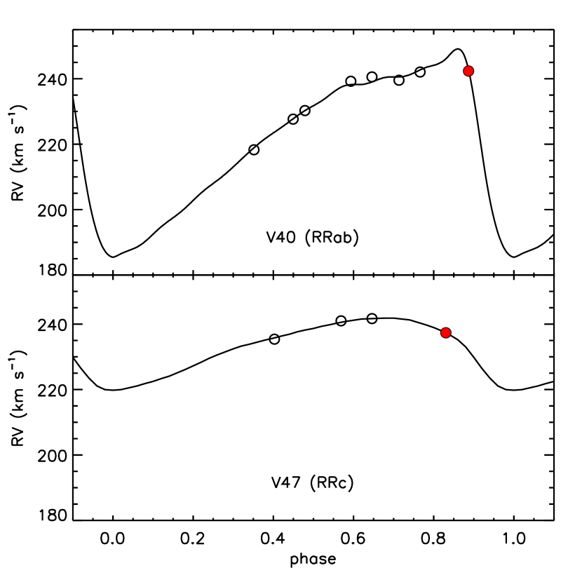
Figure 3: Results of the minimization procedure to phase multiple radial velocity measurements. The template curves by Sesar 2012 (RRab, top panel) and by Sneden et al. 2017 (RRc, bottom panel) are used as a reference to phase GIRAFFE (open black circles) and M2FS (filled red circles) observations.

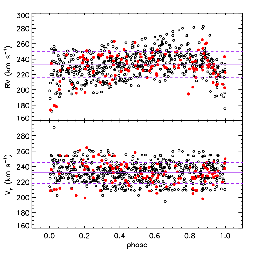
Figure 4: Top panel: instantaneous radial velocity vs. phase for all the RRLs in the M2FS (red filled circles) and in the GIRAFFE (black open circles) samples. Average velocity and $1\sigma$ dispersion are shown with purple lines. Bottom panel: as on top, but for the systemic velocity $V_{\gamma}$.

4 Abundance analysis

We used an equivalent width (EW) analysis method to derive atmospheric parameters, metallicities and relative abundances from the M2FS sample spectra.

4.1 Methodology

We selected the 140 atomic transitions listed in Table 2 from a collection of laboratory measurements and reverse solar analysis. This set of lines includes all of the transitions used in Paper I (see their Table 3 and references therein), augmented by some other lines that are detectable in the more metal-rich RRLs of $\omega$ Cen. We measured the EWs of these lines by means of a multi-gaussian fitting performed with the pyEW code developed by M. Adamow. Highly asymmetric lines were discarded, as well as too weak (EW$\leq$15 mÅ) or too strong (EW$\geq$180 mÅ) lines. The measurement error $\epsilon$ on the EW, for each absorption line, can be estimated using the relation by Venn et al. (2012)

$$\epsilon=(S/N)^{-1}\times\sqrt{1.5\times FWHM\times\delta x}+0.1\times EW$$ (3)

where $\delta x$ is the pixel size of the instrument (180 mÅ). We obtained an average error for the entire sample $\epsilon$ $\simeq$ 8 mÅ. As a final step, we used the LTE line analysis code MOOG, implemented in the Python wrapper pyMOOGi (Adamow, 2017), to estimate atmospheric parameters ($T_{\rm eff}$, log g, $\xi_{\rm turb}$, [Fe/H]) and some relative abundances, using models interpolated from a grid of $\alpha$-enhanced ($+$0.4 in the log) atmospheres (Castelli & Kurucz, 2003). The effective temperature was estimated by minimizing the dependence of the abundances on the excitation potential (EP), for the individual Fe i lines. The surface gravity was estimated by forcing the balance between the neutral and the ionized iron line abundances. Finally, the microturbulence was estimated by minimizing the dependence of the abundances on the reduced equivalent width, RW $\equiv$ log(EW/$\lambda$), for the individual Fe i lines.

Table 2: Line list and atomic parameteres.

$\lambda$	Species	EP	log($gf$)
(Å)		(eV)	(dex)
4702.991	Mg i	4.346	$-$0.44
5172.684	Mg i	2.712	$-$0.39
5183.604	Mg i	2.717	$-$0.17
5265.556	Ca i	2.523	$-$0.26
5031.021	Sc ii	1.357	$-$0.40
5239.813	Sc ii	1.456	$-$0.77
4981.731	Ti i	0.848	$+$0.57
4999.503	Ti i	0.825	$+$0.32
5064.653	Ti i	0.048	$-$0.94
5173.743	Ti i	0.000	$-$1.06

Table 3: Errors on iron abundances associated with errors on the paramater estimates.

Species	$\Delta$$T_{\rm eff}$	$\Delta$log g	$\Delta$$\xi_{\rm turb}$
	($\pm$500 K)	($\pm$0.5 dex)	($\pm$0.5 km s-1)
$\Delta$[Fe i/H]	$\pm$0.35	$\mp$0.01	$\mp$0.04
$\Delta$[Fe ii/H]	$\pm$0.10	$\pm$0.17	$\mp$0.07

Errors in estimating the atmospheric parameters also reflect in the estimated abundances. Table 3 shows the effects on iron abundance due to typical atmospheric variations occurring along the entire pulsation cycle of a RRL star (For et al., 2011; Sneden et al., 2017). Effective temperature and surface gravity are the main sources of uncertainty for Fe i and Fe ii, respectively, whereas the impact of microturbulence is relatively small.

4.2 Metallicity scale calibration

This study and Paper I represent the first use of M2FS, with its limited spectral coverage, in a traditional abundance analysis of RRL stars. It is important to understand how the metallicity scale from our analysis compares with previous studies. To accomplish this, we used spectroscopic data from the high-resolution study of field RRLs recently reported by Chadid et al. (2017, hereinafter C17). They collected thousands of spectra for a sample of 35 field RRab stars, with the du Pont telescope at Las Campanas Observatory, over several years. Their spectra cover a very large spectral interval, in the range 3400–9000 Å, much larger than the included M2FS spectral range, with a spectral resolution $R$ $\simeq$ 27,000. We performed our analysis on a selection of 27 stacked spectra (S/N $\sim$ 100) by C17, by using only the selected iron lines in the M2FS spectral range. In Table 4, we list the model parameters from C17 and from our M2FS analysis, along with the offsets between the two metallicity estimates. The agreement in the parameter sets is excellent: defining $\Delta$X $\equiv$ X_C17 $-$ X_M2FS, we found $\langle\Delta$$T_{\rm eff}$$\rangle$ = $-$43 K ($\sigma$ = 157 K), $\langle\Delta$log g$\rangle$ = $-$0.07 ($\sigma$ = 0.29), $\langle\Delta$$\xi_{\rm turb}$$\rangle$ = $-$0.33 km s^-1 ($\sigma$ = 0.43 km s^-1), and $\langle\Delta$[Fe/H]$\rangle$ = $-$0.02 ($\sigma$ = 0.11). Most importantly, our M2FS-based Fe abundances are in very good agreement with the values obtained from the more comprehensive spectra of C17 (see Figure 5). A small offset can be noticed only for two out of the three C17 most metal-rich spectra, however, the differences are within 3$\sigma$ from the mean. The difference of the third spectrum is still within 1$\sigma$. We can conclude that we are working on the same metallicity scale.

An additional calibration was performed in Paper I, in which the same kind of analysis, applied to the RRLs in the monometallic globular cluster NGC 3201, gave comparable results with previous studies based on non-variable red giant stars.

Table 4: Calibrating stars and estimated parameters.

		C17				M2FS
Star	phase	$T_{\rm eff}$	log g	$\xi_{\rm turb}$	[Fe/H]	$T_{\rm eff}$	log g	$\xi_{\rm turb}$	[Fe/H]	$\Delta$[Fe/H]
		K	cgs	km s-1	dex	K	cgs	km s-1	dex	dex
DN Aqr	0.247	6100	1.80	3.00	$-$1.78	6400	2.20	3.80	$-$1.69	$-$0.09
DN Aqr	0.366	6100	1.80	2.80	$-$1.74	6000	1.70	3.45	$-$1.85	+0.11
SW Aqr	0.280	6500	1.90	2.90	$-$1.40	6500	2.00	2.90	$-$1.39	$-$0.01
SW Aqr	0.413	6200	2.00	2.90	$-$1.34	6600	2.70	3.90	$-$1.10	$-$0.24
X Ari	0.301	6200	1.90	2.80	$-$2.66	6300	2.00	3.50	$-$2.69	+0.03
X Ari	0.374	6100	2.15	2.80	$-$2.61	6300	2.50	3.90	$-$2.56	$-$0.05
X Ari	0.470	6000	1.90	2.80	$-$2.58	6000	1.80	3.05	$-$2.60	+0.02
RR Cet	0.335	6100	1.70	2.90	$-$1.49	6250	2.10	3.15	$-$1.39	$-$0.10
RR Cet	0.554	5950	1.70	3.10	$-$1.63	6000	2.10	3.50	$-$1.56	$-$0.07
SX For	0.308	6000	1.70	2.70	$-$1.79	6100	2.00	2.75	$-$1.72	$-$0.07
SX For	0.363	6000	1.70	2.80	$-$1.80	6000	1.70	2.90	$-$1.78	$-$0.02
SX For	0.454	5950	1.70	2.80	$-$1.80	5800	1.60	2.95	$-$1.87	+0.07
V Ind	0.323	6400	2.00	2.70	$-$1.54	6200	1.80	2.70	$-$1.74	+0.20
V Ind	0.396	6200	2.00	2.80	$-$1.64	6300	2.20	2.65	$-$1.58	$-$0.06
V Ind	0.471	6200	2.10	2.70	$-$1.62	6100	2.00	2.50	$-$1.67	+0.05
SS Leo	0.314	6200	2.10	2.90	$-$1.86	6200	2.20	3.10	$-$1.87	+0.01
SS Leo	0.410	6100	2.10	2.80	$-$1.88	6100	2.00	3.50	$-$1.92	+0.04
SS Leo	0.557	6000	1.90	2.90	$-$1.91	6000	1.60	3.90	$-$1.98	+0.07
ST Leo	0.217	6650	2.00	3.00	$-$1.28	6900	2.10	3.20	$-$0.97	$-$0.31
ST Leo	0.316	6300	1.70	2.70	$-$1.28	6500	2.00	3.30	$-$1.16	$-$0.12
ST Leo	0.452	6150	2.10	2.80	$-$1.38	6000	1.50	2.75	$-$1.43	+0.05
VY Ser	0.229	6200	1.85	2.90	$-$1.91	6200	2.10	2.80	$-$1.95	+0.04
VY Ser	0.293	6200	1.85	2.90	$-$1.86	6000	1.60	3.00	$-$2.00	+0.14
VY Ser	0.366	6100	1.85	2.80	$-$1.86	6100	1.70	2.20	$-$1.85	$-$0.01
W Tuc	0.284	6350	1.75	3.00	$-$1.74	6650	2.20	3.85	$-$1.53	$-$0.21
W Tuc	0.397	6100	1.85	3.00	$-$1.72	6000	1.50	3.25	$-$1.78	+0.06
W Tuc	0.475	6100	1.85	3.00	$-$1.80	6100	1.90	3.60	$-$1.82	+0.02

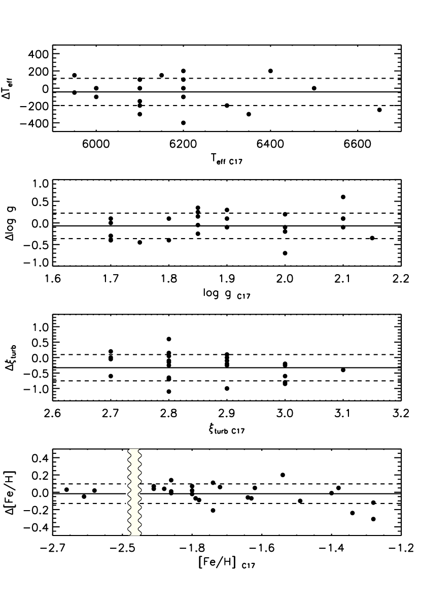
Figure 5: Difference in atmospheric parameters and iron abundance between the calibrating sample by C17 (limited to the M2FS spectral range) and our estimates for the same sample, as a function of metallicity ($\Delta$X = X_C17 $-$ X_M2FS). The mean and 1$\sigma$ are shown with solid and dashed lines. The vertical wavy lines in the last panel break the plot for convenience, since there are no objects in the interval $-2.5\lesssim$ [Fe/H] $\lesssim-2.0$.

4.3 Stellar Parameters

A total of 58 M2FS $\omega$ Cen spectra (57 objects) showed enough useful lines to perform a full spectroscopic parameter determination and abundance analysis. Figure 6 compares the relation $T_{\rm eff}$–log g for our M2FS sample (filled red circles), with the parameters obtained by For et al. (2011) and Sneden et al. (2017) for field RRLs (open black marks). The agreement of the two samples is good, with a few exceptions. In particular, two stars (V91 and V125) appear cooler than the bulk of the data. However, a visual inspection of the spectra does not give any argument to reject these stars as non-RRLs, so they are kept in the sample.

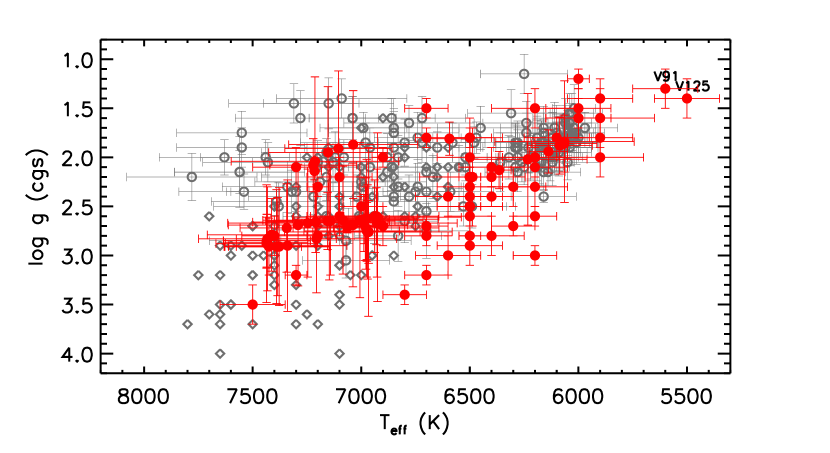
Figure 6: $T_{\rm eff}$ vs log g estimated with the EW method for our cluster RRLs (filled red circles) and a sample of literature values for field RRab (For et al., 2011, open black circles) and field RRc (Sneden et al., 2017, open black diamonds). Note that the axis orientation is reversed, to resemble the structure of a HR diagram.

Another 51 M2FS spectra did not have enough iron lines to retrieve reliable atmospheric parameters with the EW method. The S/N ratio of the spectra is quite homogeneous. The lack of lines is caused either by the low metallicity of the target, or to a hotter pulsation phase, or both. In particular, many of them did not have enough measurable Fe i lines to estimate effective temperature from Boltzmann excitation equilibrium, and others did not have any Fe ii lines to estimate surface gravity from Saha ionization equilibrium. However, we were able to estimate average parameters starting from their phase. For et al. (2011) analysed 11 field RRab, covering their entire pulsation cycles with multiple observations, showing that the atmospheric parameters have a relatively slow and regular variation along the pulsation cycle. The same applies to the 19 RRc analysed by Sneden et al. (2017). However, the two quoted groups show, at fixed pulsation phase, a significant difference in the spread for which we do not have yet an explanation (see Figure 7). Both the samples were collected at the du Pont telescope and were analysed with the same approach adopted by C17. This guarantees that we are still in the same calibration system as shown in Section 4.2. We applied the PEGASUS (PEriodic GAuSsian Uniform and Smooth fit) procedure described by Inno et al. (2015) to fit the atmospheric parameter distributions as a function of phase (solid lines in Figure 7). This was applied to the two individual samples of RRab and RRc, to obtain phase average parameters (hereinafter called PAP) to be used in the abundance determinations. The fitting function is in the form

$$y(\phi)=A_{0}+\sum_{i=1}^{N}A_{i}\ e^{-B_{i}\sin^{2}(\pi(\phi-\Phi_{i}))}$$ (4)

Table 5: Polynomial coefficients of the atmospheric parameter fitting functions.

	RRab			RRc
coeff.	$T_{\rm eff}$	log g	$\xi_{\rm turb}$	$T_{\rm eff}$	log g	$\xi_{\rm turb}$
$N$	5	3	6	5	5	4
$A_{0}$	106019	1.89243	2.71275	14383.4	2.58097	2.55349
$A_{1}$	$-$489.403	$+$0.431386	$+$0.620255	$-$440.029	$+$0.335342	$+$0.103329
$A_{2}$	$-$98093.6	$-$0.0834223	$-$0.0470036	$-$7261.09	$-$0.243433	$-$0.209276
$A_{3}$	$-$3760.66	$-$0.0719636	$+$0.21354	$-$55.011	$+$0.305311	$+$0.0910824
$A_{4}$	$-$813.769	…	$+$0.332713	$-$26.8128	$+$0.0202035	$+$0.19808
$A_{5}$	$-$1071.11	…	$+$0.594971	$-$16.9569	$+$0.0280391	…
$A_{6}$	…	…	$+$0.192962	…	…	…
$B_{1}$	19.3373	16.5656	3.17812	2.17685	2.2762	5.32572
$B_{2}$	0.0309723	7.78696	18.4264	0.0714892	7.73026	9.36127
$B_{3}$	0.943952	3.36144	17.8028	13.8483	9.66563	12.0717
$B_{4}$	10.3451	…	4.28953	15.0278	30.0616	9.83077
$B_{5}$	3.40488	…	4.6093	32.1722	65.5694	…
$B_{6}$	…	…	18.6277	…	…	…
$\Phi_{1}$	0.893882	0.932017	0.685243	0.649517	0.843868	0.398946
$\Phi_{2}$	0.500645	0.121129	0.292199	0.325824	0.525006	0.947203
$\Phi_{3}$	0.0963617	0.500979	0.892172	0.54464	0.477258	0.759689
$\Phi_{4}$	0.819111	…	0.14965	0.360766	0.234945	0.558797
$\Phi_{5}$	0.716676	…	0.825808	0.922283	0.402275	…
$\Phi_{6}$	…	…	0.0919317	…	…	…

where $y$ is one of the atmospheric parameters ($T_{\rm eff}$, log g, $\xi_{\rm turb}$) and $\phi$ is the pulsation phase. All the coefficients are provided in Table 5. Unfortunately, the errors based on this approach are about one order of magnitude larger than those based on a EW analysis, for two reasons.

i) The atmospheric parameters are the average ones, and their standard deviations can be as high as $\sigma_{T_{\text{eff}}}\simeq$ 400 K, $\sigma_{\log g}\simeq$ 0.6 dex, $\sigma_{\xi_{\text{turb}}}\simeq$ 0.6 km s^-1, especially for the first overtone mode and during the phases of maximum light. This causes uncertainties in the abundances up to 0.4–0.5 dex (see Table 3).

ii) The spectra are not good candidates for a full EW analysis due to the paucity of good lines. This means that it is more difficult to decide whether a line is good or not with respect to the others, simply because there are few lines to compare with. Indeed, in a group of tens of lines, an outlier is immediately identified and removed. At the contrary, with only one or two lines it is not possible to exclude any value.

However, this approach gives better results than an estimate of the parameters based on photometric colors, as used, for example, by Sollima et al. (2006) and Johnson & Pilachowski (2010). To confirm that, we applied both the PAP and the photometric approach to the sample of RRLs for which we spectroscopically estimated the atmospheric parameters. For the photometric approach, we used the parametrizations defined by Johnson & Pilachowski (2010), with the light curves in V and K_s collected by Braga et al. (2016, 2018). The microturbulence was defined by minimizing the abundance dependence on the reduced EW, once fixed $T_{\rm eff}$ and log g. The average differences, in terms of the atmospheric parameters, between the spectroscopic and the photometric estimates, confirm that the PAP appears to be more accurate. Indeed, defining $\Delta X_{\text{PE}}\equiv X_{\text{PAP}}-X_{\text{EW}}$ and $\Delta X_{\text{phE}}\equiv X_{\text{photometric}}-X_{\text{EW}}$, where $X$ represents one of the atmospheric parameters, we found $\langle\Delta\mbox{$T_{\rm eff}$}_{\text{,PE}}\rangle\simeq$ 240 K, $\langle\Delta\mbox{$T_{\rm eff}$}_{\text{,phE}}\rangle\simeq$ 370 K, $\langle\Delta\mbox{log~{}{\it g}}_{\text{PE}}\rangle\simeq$ 0.04, $\langle\Delta\mbox{log~{}{\it g}}_{\text{phE}}\rangle\simeq$ 0.6, $\langle\Delta\mbox{$\xi_{\rm turb}$}_{\text{,PE}}\rangle\simeq$ 0.5 km s^-1, $\langle\Delta\mbox{$\xi_{\rm turb}$}_{\text{,phE}}\rangle\simeq$ 0.08 km s^-1. The parameter dispersions in the two approaches are similar, of the order of $\sigma_{\text{\mbox{$T_{\rm eff}$}}}\simeq$ 500 K, $\sigma_{\text{\mbox{log~{}{\it g}}}}\simeq$ 0.6, $\sigma_{\text{\mbox{$\xi_{\rm turb}$}}}\simeq$ 0.5 km s^-1. We then applied the PAP approach to retrieve the abundances for the additional 51 RRLs.

For the remaining four spectra, no abundance analysis was possible because of the absence of useful lines or of phase information.

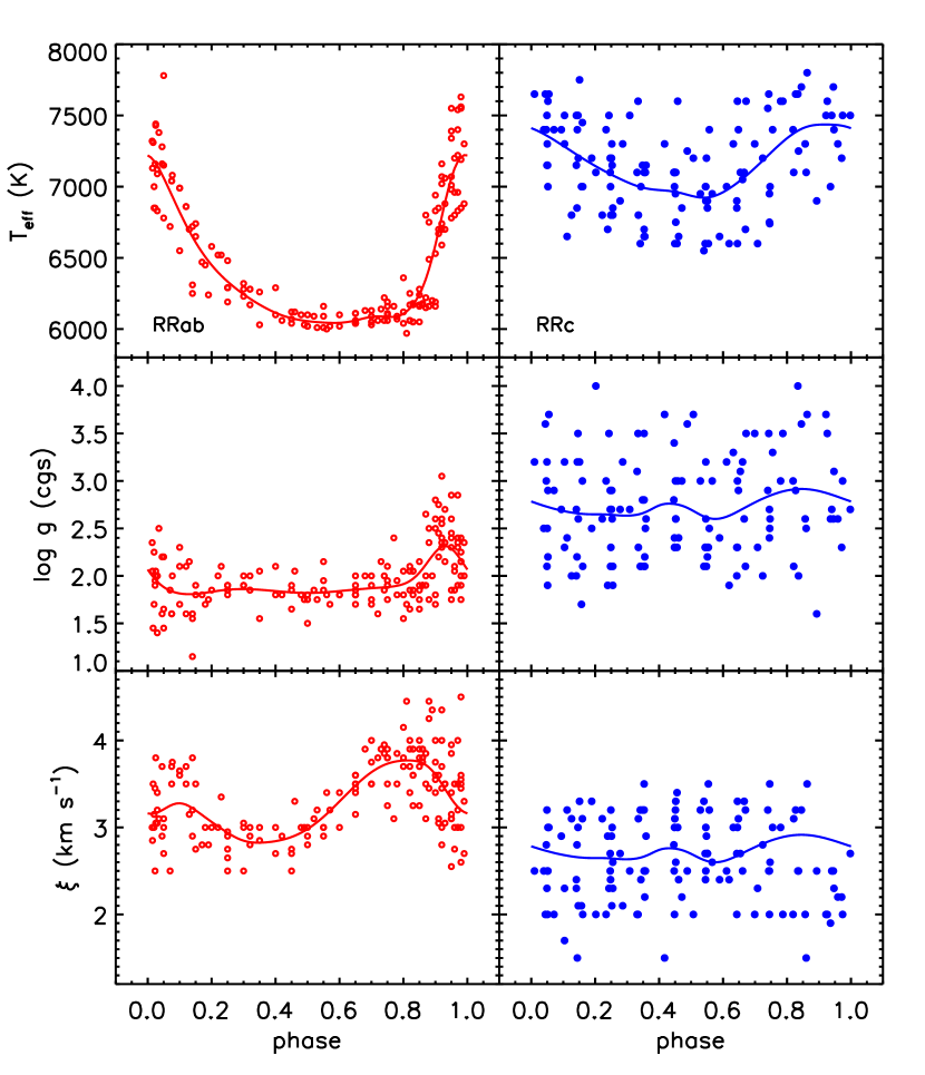
Figure 7: Atmospheric parameters vs. phase for RRab (For et al., 2011, left panels) and RRc (Sneden et al., 2017, right panels). Polynomial fits on the different samples are shown with solid lines (see text for more details).

5 Metallicity Distribution

The iron abundance estimates for the individual stars are listed in Table 6. The sample of 57 RRLs for which we applied a full spectroscopic analysis based on the EW method shows an average cluster metallicity $\langle$[Fe/H]$\rangle$ = $-1.76\pm 0.05$ and a large star-to-star dispersion $\sigma=0.36$, as expected for $\omega$ Cen Freeman & Rodgers (1975); Pancino et al. (2000); Calamida et al. (2009); Bono et al. (2019). As shown in Figure 8, top panel, our sample has its metallicity peak at about [Fe/H] = $-$1.9 and a pronounced tail toward higher metallicities, up to [Fe/H] = $-$0.85. The low metallicity tail is much less evident, with the most metal-poor RRL estimated at [Fe/H] = $-$2.53.

Before taking into account the 51 additional RRLs obtained with the PAP approach, we performed a further calibration by computing, for the RRLs in the EW sample, the corresponding iron abundances with the PAP method. In Figure 9, we plotted the difference in [Fe/H] between the two approaches, for the same stars, as a function of the iron abundance estimated with the PAP approach. There is clearly a large spread in the points, because the average atmospheric parameters can have higher or lower values than the real ones. Moreover, the parametrization for the RRab appears very promising, with a difference between the two approaches very close to zero, whereas the RRc appear, on average, more metal-rich with the PAP approximation. We therefore applied a zero point calibration to the PAP sample of $\omega$ Cen RRLs, according to the pulsation type, to make it consistent with the more accurate spectroscopic one. We also applied the same kind of correction to all the other elements, after performing a similar calibration based on their [X/H] abundances. Figure 8, middle panel, shows the histogram for the entire M2FS sample (black thick line) after the calibration, together with the two subsamples: the EW (orange filled area) and the PAP (purple shaded area). For the joint EW and PAP samples, we derived $\langle$[Fe/H]$\rangle$ = $-1.82\pm 0.03$ ($\sigma$ = 0.33). This mean value is only 0.06 dex lower than that derived with the pure EW analysis. Once again, the distribution peaks at about [Fe/H] = $-$1.9, with a longer metal-rich tail and a shorter metal-poor one.

Table 7 shows the mean iron content of the two RRL populations, RRab and RRc, with the different approaches adopted. It can be noticed that the EW method produces very similar results for both RRab and RRc, with a difference in the average iron content limited to 0.03 dex. At the contrary, the PAP method produces a RRab population that is 0.13 dex more metal-rich than the RRc one. In particular, the RRab sample has the same average abundance ($\langle$[Fe/H]$\rangle$ = $-$1.78) for both methods, whereas the RRc sample is more metal-poor in the PAP sample ($\langle$[Fe/H]$\rangle$ = $-$1.91) than in the EW one ($\langle$[Fe/H]$\rangle$ = $-$1.75). However, a lower metallicity for the PAP sample is expected, since the method is applied to those spectra with a limited number of lines.

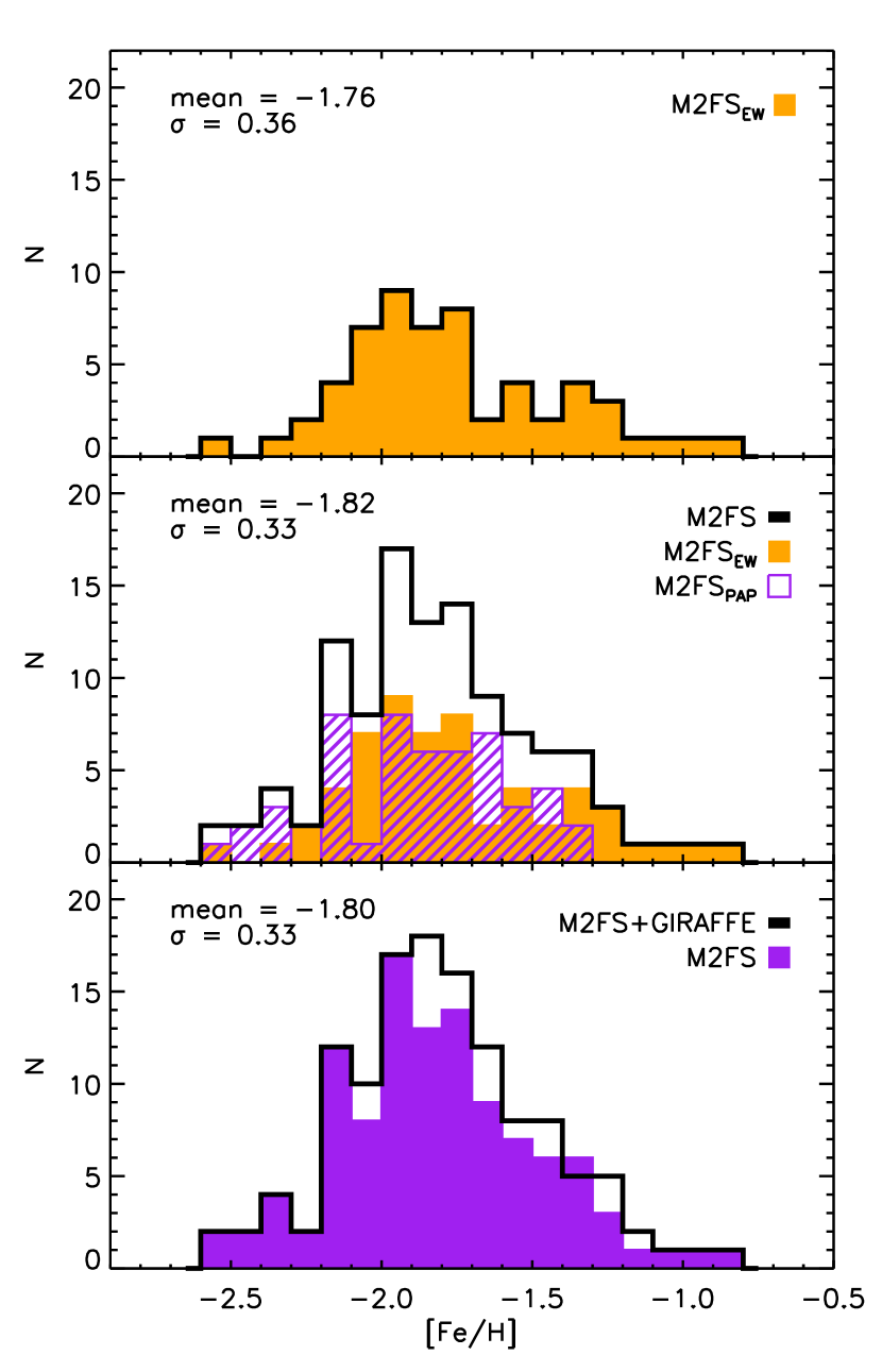
Figure 8: Top panel: metallicity distribution for the M2FS sample of RRLs in $\omega$ Cen, whose parameters were estimated with the EW approach. Middle panel: metallicity distribution for the full sample of M2FS RRLs (black thick line). The orange filled area is the same as in the top panel, showing the sample estimated with the EW approach. The purple shaded area shows the sample estimated with the PAP approach. Bottom panel: metallicity distribution of the entire sample of RRLs collected with M2FS and GIRAFFE (black thick line). The purple filled area is the same total M2FS sample shown in the middle panel.

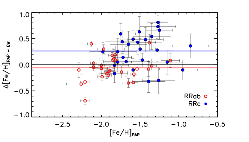
Figure 9: Calibration of the metallicity scale obtained with the EW and the PAP approach for the M2FS sample RRLs. The mean difference of the two samples was used to correct the PAP sample.

Table 6: Iron abundances for the considered samples of $\omega$ Cen RRLs. Mean value, standard deviation, and number of stars for each sample are listed at the bottom.

ID	[Fe/H]EW	[Fe/H]PAP	[Fe/H]GIRAFFE	$n$	[Fe/H]tot
V4	…	$-$1.82 $\pm$ 0.10	…	…	$-$1.82 $\pm$ 0.10
V5	$-$1.40 $\pm$ 0.02	…	$-$1.51 $\pm$ 0.29	2	$-$1.40 $\pm$ 0.03
V7	$-$1.76 $\pm$ 0.03	…	…	…	$-$1.76 $\pm$ 0.03
V8	$-$2.19 $\pm$ 0.07	…	…	…	$-$2.19 $\pm$ 0.07
V10	$-$2.23 $\pm$ 0.04	…	…	…	$-$2.23 $\pm$ 0.04
V11	$-$1.88 $\pm$ 0.05	…	…	…	$-$1.88 $\pm$ 0.05
V12	…	$-$2.37 $\pm$ 0.04	…	…	$-$2.37 $\pm$ 0.04
V15	…	…	$-$1.68 $\pm$ 0.35	3	$-$1.68 $\pm$ 0.35
V16	…	$-$2.00 $\pm$ 0.11	…	…	$-$2.00 $\pm$ 0.11
V18	…	$-$1.89 $\pm$ 0.52	…	…	$-$1.89 $\pm$ 0.52
$\omega$ Cen	$-$1.76 $\pm$ 0.05	$-$1.87 $\pm$ 0.04	$-$1.71 $\pm$ 0.04		$-$1.80 $\pm$ 0.03
$\sigma$	0.36	0.30	0.28		0.33
$N$	57	51	44		125

Table 7: Mean iron abundance and standard deviation for the analysed samples, with distintion between different RRL pulsation modes. The number of stars for each subsample is also indicated.

	M2FS${}_{\text{EW}}$			M2FS${}_{\text{PAP}}$			GIRAFFE
Mode	$N$	$\langle$[Fe/H]$\rangle$	$\sigma$	$N$	$\langle$[Fe/H]$\rangle$	$\sigma$	$N$	$\langle$[Fe/H]$\rangle$	$\sigma$
RRab	28	$-$1.78	0.34	14	$-$1.78	0.26	37	$-$1.68	0.28
RRc	29	$-$1.75	0.39	37	$-$1.91	0.31	7	$-$1.83	0.26

5.1 The GIRAFFE sample

Among the $\sim$500 GIRAFFE spectra for which we measured a radial velocity, only a limited sample of 99 spectra (44 objects, 27 in common with the M2FS sample) showed high enough S/N (40 $\lesssim$ S/N $\lesssim$ 110) and useful iron lines to perform accurate EW measurements. However, the number of iron lines was too limited for a spectroscopic determination of the atmospheric parameters. In particular, they lacked useful Fe ii lines to balance the surface gravity. Therefore, we applied the PAP approach to estimate the atmospheric parameters, then the abundances, for all the stars with available phase information and good enough iron lines.

As a first step, we averaged the abundances for the stars with multiple GIRAFFE measurements. Then, we compared the stars in common between the GIRAFFE and the M2FS samples. This defined a zero point calibration for RRab and RRc, used to move the entire GIRAFFE sample to the M2FS, spectroscopic, metallicity scale. After the scaling, we performed a weighted averaged of the abundances for the stars with multiple measurements of the two spectrographs (last column of Table 6), assuming the inverse square of the error as weight. We ended with a sample of 125 RRLs, whose distribution is shown in the bottom panel of Figure 8. The shape of the distribution still remains essentially the same, with $\langle$[Fe/H]$\rangle$ = $-1.80\pm 0.03$ and a dispersion $\sigma$ = 0.33 dex.

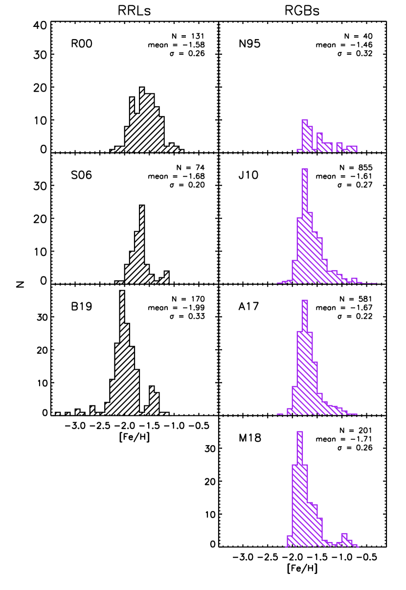
Figure 10: Metallicity distribution for the sample of RRLs (black, left column) and RGBs (purple, right column) in $\omega$ Cen, available in the literature (R00: Rey et al. 2000; S06: Sollima et al. 2006; B19: Bono et al. 2019; N95: Norris & Da Costa 1995; J10: Johnson & Pilachowski 2010; A17: An et al. 2017; M18: Mucciarelli et al. 2018, 2019). J10, A17, and M18 have been scaled to a maximum height of 35 for plotting reasons. They should be multiplied by $\sim$5, $\sim$4, and $\sim$1.5 respectively, to obtain the real scale. The number of stars in the sample, the mean, and the standard deviation are labelled in the top right corner.

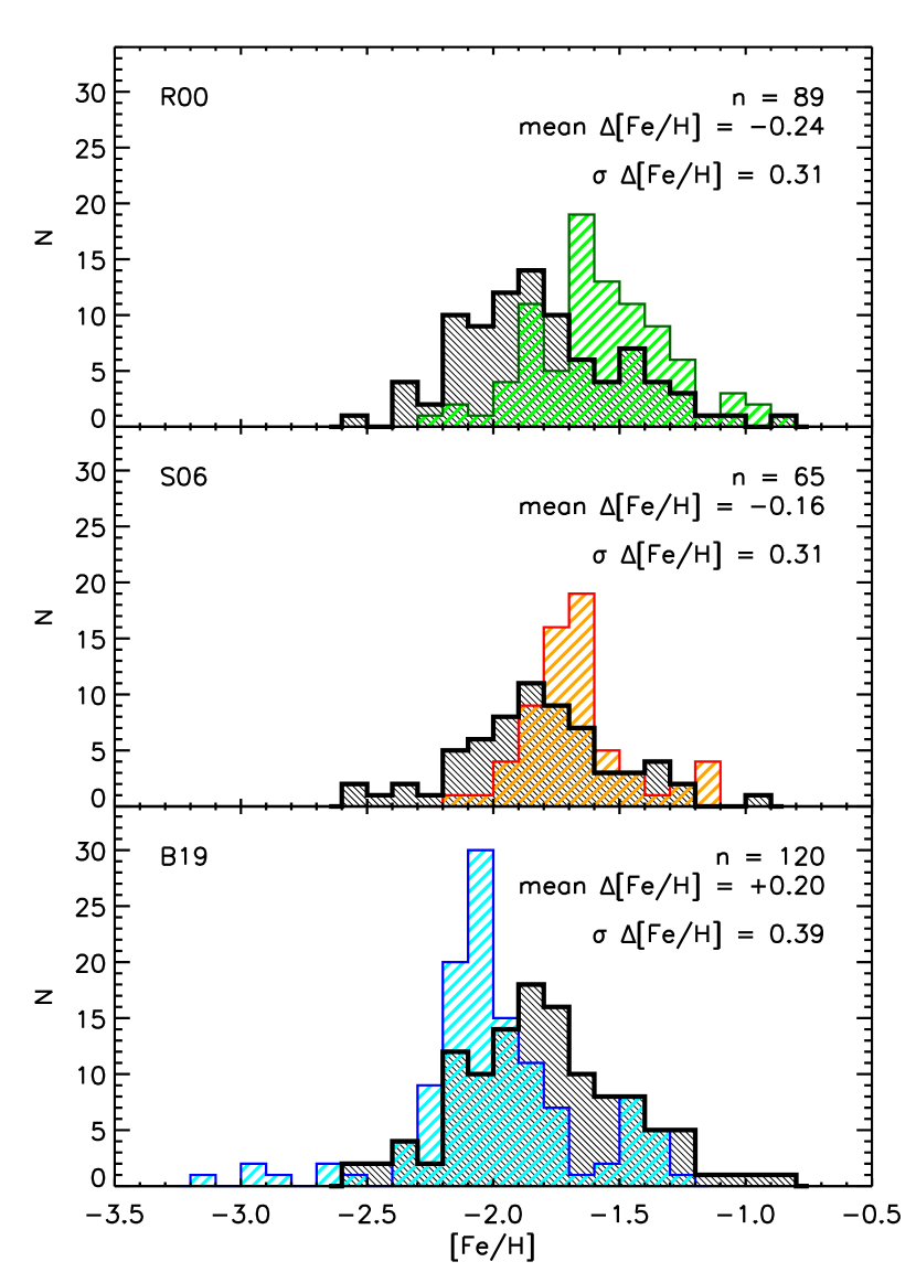
Figure 11: Comparison of the metallicity distribution for our entire $\omega$ Cen sample (M2FS+GIRAFFE, black) and the RRL samples available in the literature (R00: Rey et al. 2000; S06: Sollima et al. 2006; B19: Bono et al. 2019). For each panel, only the stars in common ($\boldsymbol{n}$) between the two works are considered. Mean and standard deviation of the differences among the two samples ($\Delta$[Fe/H] = this work $-$ literature) are labelled on the top right corners of each panel.

5.2 Comparison with the literature

The large dispersion in the metallicity of $\omega$ Cen is a well known attribute that has been investigated for decades. Previous studies of both RGBs (Norris & Da Costa, 1995; Johnson & Pilachowski, 2010; An et al., 2017; Mucciarelli et al., 2018, 2019) and RRLs (Butler et al., 1978; Gratton et al., 1986; Rey et al., 2000; Sollima et al., 2006; Bono et al., 2019) clearly showed metallicity spreads between 0.20 and 0.45 dex. In Figure 10, we collected the [Fe/H] distributions for the largest and most recent studies. With the exception of Rey et al. (2000, hereinafter R00), whose distribution is essentially symmetric, the histograms show the longer metal-rich tail distribution also found in the present study. However, the RRL based analysis of Sollima et al. (2006, hereinafter S06) and Bono et al. (2019, hereinafter B19), as well as the RGB analysis by Mucciarelli et al. (2018, 2019), show the metal-rich tail as a separated secondary peak, whereas the current sample shows either a metal-rich secondary peak for [Fe/H] $\geq$ $-$1.5 (M2FS_EW) or a well defined metal-rich shoulder (M2FS+GIRAFFE). This was already noticed, among the others, by Norris et al. (1996, 1997) with Ca abundance and kinematics data, but we will discuss this point in more detail in Section 8.

It is worth mentioning that the iron distribution peak in the literature is, on average, $\sim$0.2 dex more metal-rich than our estimate, with the exception of B19 who found a slightly more metal-poor peak. These differences are mainly due to the techniques used to estimate the atmospheric parameters. Indeed, S06, Johnson & Pilachowski (2010), and An et al. (2017) used photometrically estimated parameters that, as already mentioned in Section 4.3, give slightly higher $T_{\rm eff}$ and log g. Comparing our GIRAFFE analysis with the sample by S06, that is included in our sample, we found an average difference, for the stars in common, $\Delta$[Fe/H]${}_{\text{GIRAFFE - S06}}$ = $-$0.13. Since this difference can not be due to the spectra, it can only be related to the applied technique. Finally, R00 used the photometric hk index to indirectly estimate the metallicity, while B19 used a technique based on PLZ theoretical predictions. The comparison of the literature results with our entire $\omega$ Cen sample (M2FS+GIRAFFE) is shown in Figure 11, only considering the stars in common among each work and this one. The average differences in [Fe/H] are $\langle\Delta$[Fe/H]$\rangle_{\text{this work--R00}}$ = $-$0.24 (n = 89, $\sigma$ = 0.31), $\langle\Delta$[Fe/H]$\rangle_{\text{this work--S06}}$ = $-$0.16 (n = 65, $\sigma$ = 0.31), and $\langle\Delta$[Fe/H]$\rangle_{\text{this work--B19}}$ = $+$0.20 (n = 120, $\sigma$ = 0.39).

6 The $\alpha$-elements: Mg, Ca, and Ti

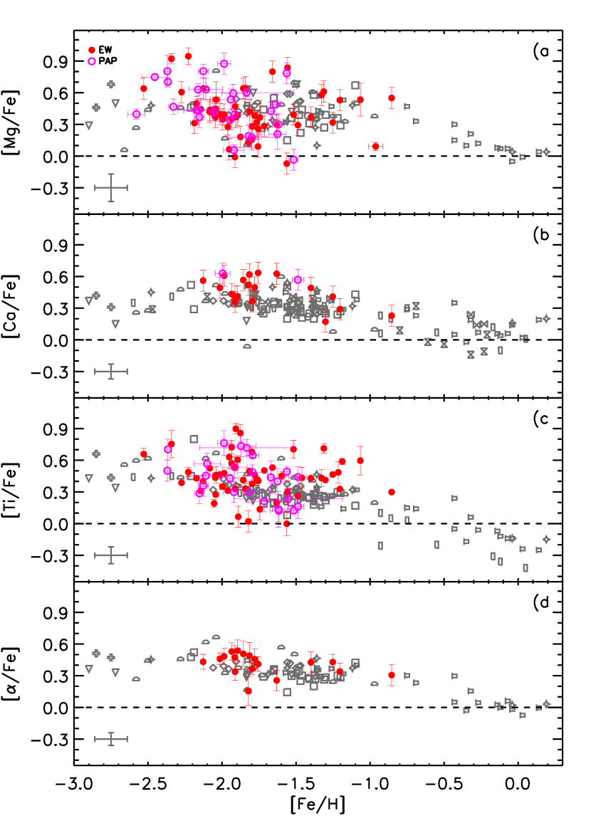
Figure 12: $\alpha$-elements vs. iron abundances for the RRLs in $\omega$ Cen. The stars analysed with the EW approach are marked with red filled circles, those analysed with the PAP approach are marked with magenta open circles. The black symbols mark the field halo RRLs collected with high-resolution spectroscopy from the literature. In each panel, the black error bar on bottom left corner shows the mean individual errors for the literature sample.

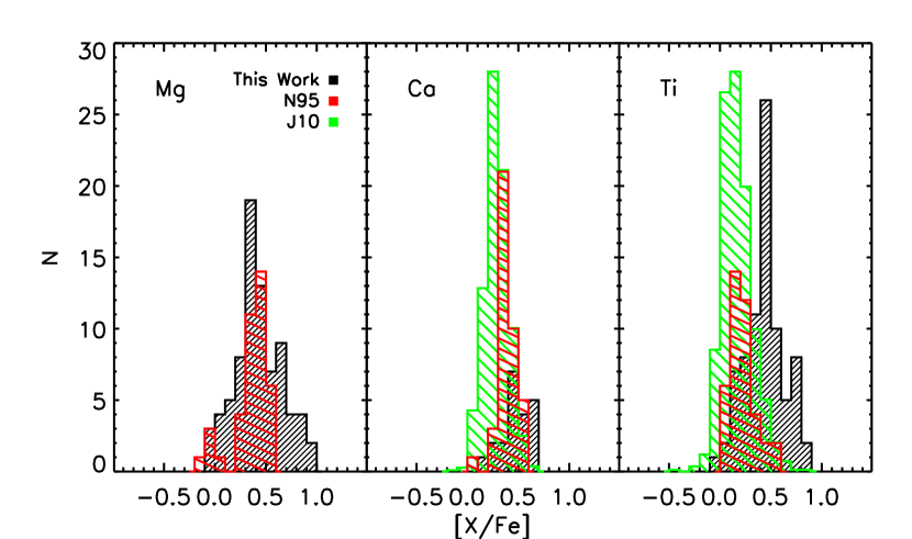
Figure 13: $\alpha$-elements distribution for RGB stars in $\omega$ Cen (N95: Norris & Da Costa 1995; J10: Johnson & Pilachowski 2010), compared with our RRLs sample. J10 has been scaled to a maximum value of 28 for plotting reason.

Figure 14: Top panel: $\alpha$-elements (Mg+Ca+Ti) vs. iron abundances for the individual RRLs in $\omega$ Cen (red filled circles). The sample is compared with Galactic globulars (filled black diamonds, Pritzl et al. 2005; Carretta et al. 2009, 2010) and field halo RRLs (open purple diamonds, same samples as in Figure 12). The solid blue line shows the log-normal fit of the two joint samples, with the 1$\sigma$ dispersion shown by the blue bar in the top left corner. Bottom panel: as on top, but compared with field halo giants (black dots, Frebel, 2010) and RHB–BHB field stars (orange–blue squares, For & Sneden, 2010). The dashed blue line shows an extrapolation of the fit toward lower iron abundances.

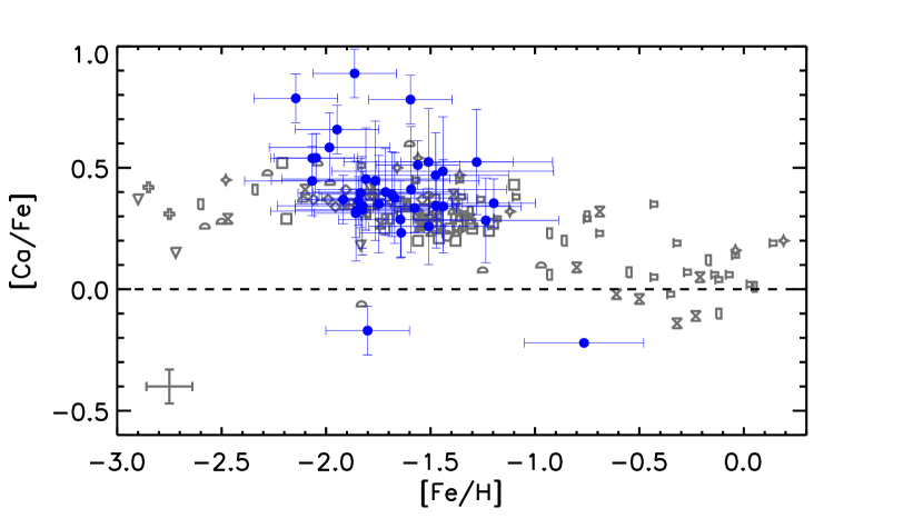
Figure 15: As in Figure 12, panel (b), but for abundances derived from the GIRAFFE spectra (blue filled circles).

Table 8: $\alpha$-, iron-peak, and s-process element abundances for the considered samples of $\omega$ Cen RRLs collected with M2FS. Mean value, standard deviation, and number of stars for each species are listed at the bottom.

ID	[Mg/Fe]	[Ca/Fe]	[Ti/Fe]	[ $\alpha$/Fe]	[Sc/Fe]	[Cr/Fe]	[Ni/Fe]	[Zn/Fe]	[Y/Fe]
V4	0.19 $\pm$ 0.10	…	…	…	…	…	…	…	…
V5	0.37 $\pm$ 0.10	0.49 $\pm$ 0.10	0.43 $\pm$ 0.05	0.43 $\pm$ 0.10	0.08 $\pm$ 0.10	0.01 $\pm$ 0.04	0.01 $\pm$ 0.10	0.30 $\pm$ 0.16	0.38 $\pm$ 0.08
V7	0.26 $\pm$ 0.10	0.63 $\pm$ 0.10	0.40 $\pm$ 0.03	0.41 $\pm$ 0.07	…	$-$0.28 $\pm$ 0.03	…	…	0.19 $\pm$ 0.10
V8	0.31 $\pm$ 0.10	…	…	…	…	0.36 $\pm$ 0.10	…	…	…
V10	0.95 $\pm$ 0.14	…	0.49 $\pm$ 0.09	…	…	0.24 $\pm$ 0.10	…	…	…
V11	0.18 $\pm$ 0.10	…	0.86 $\pm$ 0.11	…	0.66 $\pm$ 0.10	…	…	…	…
V12	0.80 $\pm$ 0.21	…	0.50 $\pm$ 0.10	…	0.33 $\pm$ 0.10	…	…	…	…
V16	…	0.63 $\pm$ 0.10	…	…	…	…	…	…	…
V18	…	…	…	…	…	…	…	…	…
V20	0.09 $\pm$ 0.10	…	0.41 $\pm$ 0.03	…	0.10 $\pm$ 0.10	0.08 $\pm$ 0.10	0.09 $\pm$ 0.12	…	$-$0.10 $\pm$ 0.10
$\omega$ Cen	0.43 $\pm$ 0.03	0.47 $\pm$ 0.03	0.44 $\pm$ 0.02	0.41 $\pm$ 0.02	0.11 $\pm$ 0.04	0.09 $\pm$ 0.02	0.06 $\pm$ 0.04	0.30 $\pm$ 0.05	0.25 $\pm$ 0.05
$\sigma$	0.22	0.13	0.19	0.10	0.21	0.18	0.17	0.11	0.31
$N$	78	21	80	18	32	52	20	6	40

The M2FS spectra cover a relatively short wavelength range, limiting the $\alpha$-element line measurements to only three species: Mg, Ca, and Ti. Titanium is not a “pure” $\alpha$-element (its dominant isotope is ⁴⁸Ti instead of ⁴⁴Ti), however, its abundance at low metallicity usually mimics those of the other $\alpha$-elements. Moreover, titanium lines are the most numerous after iron in the M2FS wavelength range, and in some cases they are the only observable ones among the $\alpha$. Indeed, up to 13 Ti i and Ti ii lines were measured in a single spectrum, whereas Mg i lines were limited to three at most, and only a single Ca i line was measured, if any. We estimated their average cluster abundances for the EW sample as $\langle$[Mg/Fe]$\rangle$ = 0.41 $\pm$ 0.03, $\langle$[Ca/Fe]$\rangle$ = 0.46 $\pm$ 0.03, and $\langle$[Ti/Fe]$\rangle$ = 0.44 $\pm$ 0.03. The dispersion of Mg is the largest one ($\sigma$ = 0.22), whereas Ca has the smallest dispersion ($\sigma$ = 0.13), but also the lowest number of measurements, and Ti lies in between ($\sigma$ = 0.19). Adding the RRLs analysed with the PAP approach does not change significantly the final results, but they double the number of stars: $\langle$[Mg/Fe]$\rangle$ = 0.43 $\pm$ 0.03, $\langle$[Ca/Fe]$\rangle$ = 0.47 $\pm$ 0.03, and $\langle$[Ti/Fe]$\rangle$ = 0.44 $\pm$ 0.02, with exactly the same dispersions as before.

Table 8 lists the individual star abundances, and Figure 12 compares them with those of the field halo RRLs, collected with high-resolution (R $\geq$ 25,000) spectroscopy, available in the literature (Clementini et al., 1995; Fernley & Barnes, 1996; Lambert et al., 1996; Kolenberg et al., 2010; For et al., 2011; Hansen et al., 2011; Liu et al., 2013; Govea et al., 2014; Pancino et al., 2015; Chadid et al., 2017; Sneden et al., 2017, more details about the literature samples can be found in the Appendix of Paper I). The agreement of the two considered samples is evident. The running mean of the two groups is the same, within the dispersion, in the metallicity range covered by the $\omega$ Cen stars, where the $\alpha$-element abundances are almost constant or slightly decreasing toward higher metallicities. We also computed the [$\alpha$/Fe] abundance for the individual RRLs as the biweight mean of the three considered element abundances (bottom panel of Figure 12). Details about this robust iterative estimator of location can be found in Beers et al. (1990). The [$\alpha$/Fe] abundance was only estimated for those RRLs showing lines of all the three elements. This limits the sample to 18 RRLs, but the homogeneity of the results is preserved. The cluster average abundance was estimated as $\langle$[$\alpha$/Fe]$\rangle$ = 0.41 $\pm$ 0.02 ($\sigma$ = 0.10).

Figure 13 compares our $\alpha$-element abundances with those derived in earlier investigations of $\omega$ Cen red giants, and there is a general agreement. It can be noticed that our estimates of Mg abundances are more scattered than those by Norris & Da Costa (1995), but with similar mean values. However, this difference can simply be caused by the different sample size (78 vs. 40 measurements). On the contrary, Ca and Ti have similar dispersions between RRLs and RGBs, but with higher abundances for our sample, especially for Ti, with respect to both Norris & Da Costa (1995) and Johnson & Pilachowski (2010). The two different populations display quite similar $\alpha$-element abundances over the entire metallicity range. To further investigate the chemical enrichment of the $\alpha$-elements in different stellar components, we also compared our results for $\omega$ Cen with similar abundances available in the literature for Galactic globular clusters (Pritzl et al., 2005; Carretta et al., 2009, 2010), field halo red/blue horizontal branch stars (RHB, BHB, For & Sneden, 2010), and kinematically selected field halo red giants (Frebel, 2010). Figure 14 shows all the previous samples and a log-normal analytical fit of their [$\alpha$/Fe] vs. [Fe/H], computed with the Equation 1 in Paper I. It is remarkable that all the observed components, which are RRLs or non-variables, and which are cluster or field stars, agree with the fit within 1$\sigma$. This suggests that all these components experienced very similar chemical enrichment histories for these $\alpha$-elements, also supporting a common old (t $\geq$ 10 Gyr) age for all of them.

From the GIRAFFE spectra, the only element other than Fe that was possible to measure with sufficient precision is Ca. We estimated [Ca/Fe] for 40 out of 44 stars in the sample, shown in Figure 15. Despite a few outliers, the average Ca abundance for the GIRAFFE spectra is in good agreement with the literature values for field halo RRLs. We estimated the average abundance for the GIRAFFE sample, excluding the evident outliers with a sigma clipping procedure, as $\langle$[Ca/Fe]$\rangle$ = 0.42 $\pm$ 0.03, with a dispersion $\sigma$ = 0.17.

7 The Iron-peak Elements: Sc, Cr, Ni, and Zn

We estimated abundances for a few heavier elements in the iron-peak group (Z = 21–30): Sc, Cr, Ni, and Zn, only observable in the M2FS spectra. There are significant differences in the number of useful lines among the four species; indeed, some of these elements are undetectable in many of the stars (Table 8). Cr is the most broadly represented element, observed in about 50% of the RRLs ($\sim$70% for the EW sample alone), with up to ten lines in the best case and at least a couple of lines for the majority of the spectra (either Cr i or Cr ii). On the other hand, Zn i was only observed in a handful of stars, especially in the metal-rich tail of the sample, with only one or two lines. Sc ii and Ni i both have few observed lines in the M2FS spectral range, but the number of RRLs showing them is between those with Cr and Zn. The average cluster abundances were estimated as $\langle$[Sc/Fe]$\rangle$ = 0.11 $\pm$ 0.04, $\langle$[Cr/Fe]$\rangle$ = 0.09 $\pm$ 0.02, $\langle$[Ni/Fe]$\rangle$ = 0.06 $\pm$ 0.04, and $\langle$[Zn/Fe]$\rangle$ = 0.30 $\pm$ 0.05.

Figure 16 shows the comparison between the abundances of the iron-peak elements for the individual $\omega$ Cen RRLs and for the field halo RRLs available in the literature (see Appendix in Paper I for more details about the literature sample). The agreement of the two groups is very good. The running means of the two samples with metallicity are nearly the same. The dispersions, in the metallicity range covered by $\omega$ Cen, are also very similar between the two groups and to those of the $\alpha$-elements, for Sc ($\sigma_{\text{\mbox{$\omega$~{}Cen}}}$ = 0.21, $\sigma_{\text{halo}}$ = 0.15), Cr ($\sigma_{\text{\mbox{$\omega$~{}Cen}}}$ = 0.18, $\sigma_{\text{halo}}$ = 0.09), Ni ($\sigma_{\text{\mbox{$\omega$~{}Cen}}}$ = 0.17, $\sigma_{\text{halo}}$ = 0.26), and Zn ($\sigma_{\text{\mbox{$\omega$~{}Cen}}}$ = 0.11, $\sigma_{\text{halo}}$ = 0.14). Once again, the chemical enrichment history of the RRLs in the Galactic halo appears to be similar for both field and cluster stars.

Our Fe-group abundances from RRL stars are also in good agreement with those derived from the RGB samples. The results obtained by Norris & Da Costa (1995) and Johnson & Pilachowski (2010) for the $\omega$ Cen RGBs (Figure 17) are in general agreement with our RRL sample, with only limited differences in the average values, suggesting similar enrichment histories for the two stellar groups.

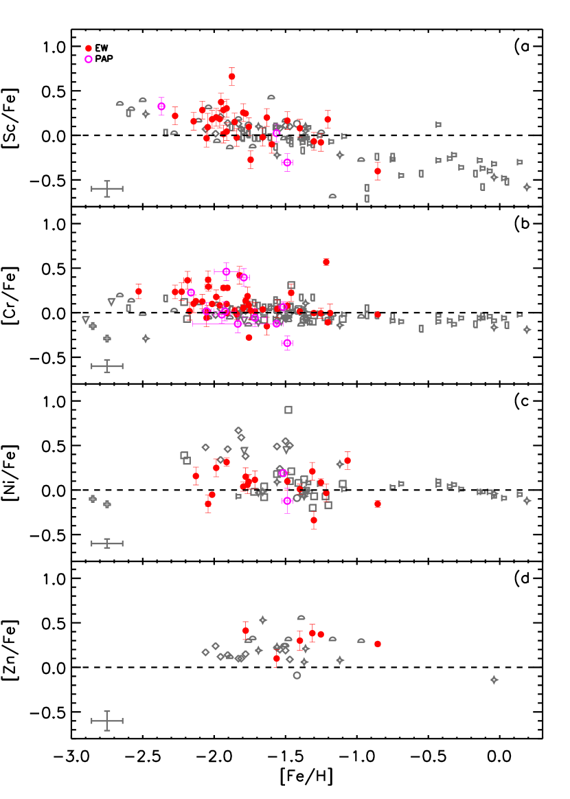
Figure 16: Iron-peak elements vs. iron abundances for the RRLs in $\omega$ Cen. The stars analysed with the EW approach are marked with red filled circles, those analysed with the PAP approach are marked with magenta open circles. The black symbols mark the field halo RRLs collected with high-resolution spectroscopy from the literature. In each panel, the black error bar on bottom left corner shows the mean individual errors for the literature sample.

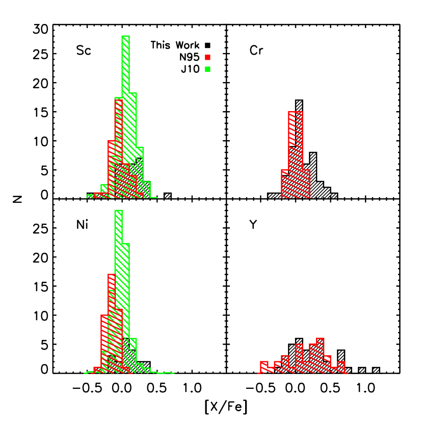
Figure 17: Iron-peak and s-process elements distribution for RGB stars in $\omega$ Cen (N95: Norris & Da Costa 1995; J10: Johnson & Pilachowski 2010), compared with our RRLs sample. Zn is not shown because missing in the RGB samples. J10 has been scaled to a maximum value of 28 for plotting reason.

8 The s-process Element: Y

Among the neutron-capture elements (Z $>$ 30), in the M2FS spectral range, only Y ii lines are easily observable in RRLs (Table 8). A couple of La ii transitions are also present, but they are too weak to produce reliably detectable lines. Indeed, synthetic spectrum tests show that these lines are not observable for [La/H] $\lesssim$ $-$0.8, even with very high S/N. Y ii lines were measured in the entire metallicity range covered by $\omega$ Cen, with an average abundance for the entire sample $\langle$[Y/Fe]$\rangle$ = 0.25 $\pm$ 0.05 and a dispersion $\sigma$ = 0.31. Figure 18 shows the comparison between the Y abundances of RRLs in $\omega$ Cen and the field halo RRLs (top panel, see Appendix in Paper I for details) and RGs (bottom panel, Frebel et al. 2010). Two groups of stars in $\omega$ Cen show different levels of Y-enhancement: about half of the sample is in very good agreement with the field stars, having about solar Y abundances; the other half of the RRLs shows a clear over-enhancement of Y, with [Y/Fe] $\gtrsim$ 0.4. Figure 19 shows the comparison of two spectra: a Y-enhanced RRL (V112, [Y/Fe] = $+$0.61, black line) and an almost solar one (V20, [Y/Fe] = $-$0.10, red line). The two stars are both RRab, observed at similar phase ($\phi$ = 0.28 and 0.36, respectively), and with similar iron abundance ([Fe/H] = $-$1.78 and $-$1.76, respectively). The two shown iron lines are, indeed, almost identical, whereas the yttrium lines are largely different one from each other.

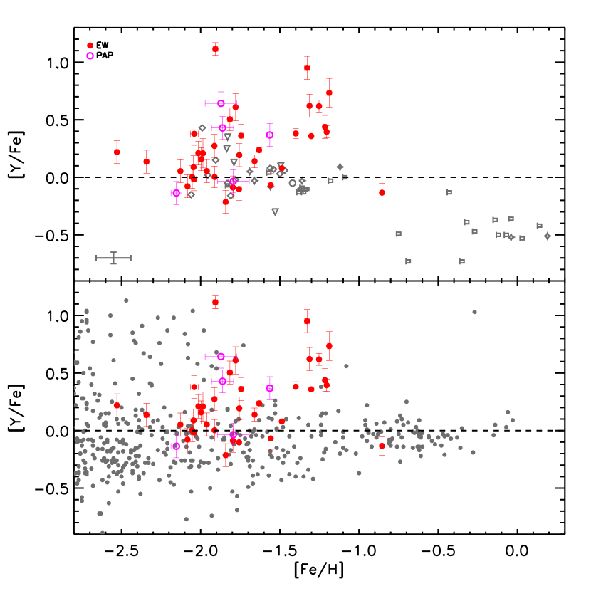
Figure 18: Top panel: yttrium vs. iron abundances for the RRLs in $\omega$ Cen. The stars analysed with the EW approach are marked with red filled circles, those analysed with the PAP approach are marked with magenta open circles. The black symbols mark the field halo RRLs collected with high-resolution spectroscopy from the literature. The black error bar on bottom left corner shows the mean individual errors for the literature sample. Bottom panel: as on top, but compared with field halo RGs (black dots, Frebel, 2010)

The Y-enhanced group of RRLs appears to be mostly the metal-rich one in $\omega$ Cen ([Fe/H] $\gtrsim$ $-$1.5), suggesting differential enrichments for two groups of RRLs. A few other objects with similar strong Y-enhancement are also observed at lower metallicity ([Fe/H] $\sim$ $-$1.8). However, they are a minor fraction of the RRLs more metal poor than [Fe/H] $\lesssim$ $-$1.5. The abrupt increase in the s-process element abundances with increasing [Fe/H] was first observed by Lloyd Evans (1983) and later confirmed by Francois et al. (1988), Paltoglou & Norris (1989), and Vanture et al. (1994), not only for Y, but also for La, Zr, Ba, and Nd. Johnson & Pilachowski (2010) estimated the La abundance for $\sim$800 RGB stars, finding a clear separation between the most metal-poor stars, with almost zero enhancement ([Fe/H] $\lesssim$ $-$1.6, [La/Fe] $\simeq$ 0.0), and the most metal-rich, La enhanced ([Fe/H] $\gtrsim$ $-$1.6, [La/Fe] $\simeq$ 0.4). The hypothesis by Smith et al. (2000) and Cunha et al. (2002) is that two different populations coexist in $\omega$ Cen, whose enrichment history was strictly related to their capability to retain the products of the low velocity ejecta of asymptotic giant branch (AGB) stars wind (rich in s-process elements), allowing a heavy self-enrichment of the second, metal-rich, stellar generation, over time scales of the order of 1 Gyr. We note that the two groups of RRLs, the solar-enhanced and the over-enhanced, show similar radial distributions from the cluster center and similar kinematic properties (radial velocity, radial velocity dispersion). However, more statistics is required before we can reach a firm conclusion.

A different scenario was advanced by Romano et al. (2007), who suggested that the self-enrichment scenario is not able to reproduce the metallicity distribution of $\omega$ Cen, and that the best hypothesis is that of $\omega$ Cen as the remnant of a dwarf spheroidal galaxy, evolved in isolation and then accreted by the Milky Way. In favour of the working hypothesis suggested by Romano et al., let us mention that the Y-enhanced RRLs appear to be an isolated group in terms of Fe and Y abundances, i.e. the current data do not suggest a steady increase in Y when moving from metal-poor to metal-rich RRLs. It is also worth mentioning that Norris et al. (1996) suggested, on the basis of a large sample of Ca abundances of $\omega$ Cen red giants, that $\omega$ Cen might be the merging of two different globulars. This kind of enrichment in s-process elements has never been observed in other Galactic RRLs, and indeed, field RRLs do not show similar Y over-abundances.

Investigations of field stars and globular clusters in dwarf galaxies suggest that only a very limited difference with respect to the Milky Way exists for Y and other s-process element abundances, showing almost zero enhancement with respect to the Sun (Tolstoy et al., 2009, and references therein). Ba abundance in the Fornax dwarf galaxy represents a remarkable exception. Letarte et al. (2010) found [Ba/Fe] $\simeq$ 0.7 for the investigated stars, more metal-rich than [Fe/H] $\simeq$ $-$1.0. However, no similar enhancement was found for Y, and the problem is still open. Even if we can not easily distinguish two separate populations from the [Fe/H] data, as was for S06 and B19, our [Y/Fe] abundances confirm that two distinct populations, one more metal-poor and the other more metal-rich than [Fe/H] $\simeq$ $-$1.5, coexist in $\omega$ Cen. However, over-enhanced RRLs are also observed at [Fe/H] $\sim$ $-$1.8, and the most metal-rich RRL in our sample shows almost solar Y abundance, so that the distinction between the two metallicity groups is not strict.

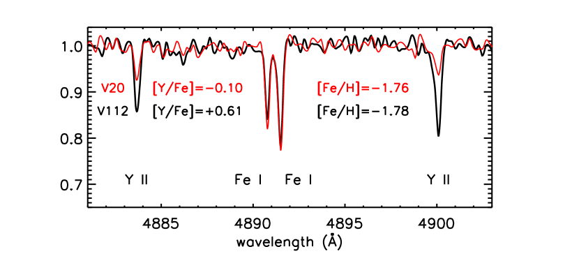
Figure 19: Comparison of two spectra for similar RRLs (same pulsation mode, almost same phase and iron abundance) but with different Y enhancement.

9 Conclusion and final remarks

We performed a large investigation of RR Lyrae stars in the globular cluster $\omega$ Cen, using high-resolution, high S/N spectroscopy. We almost doubled the current sample of optical high-resolution spectroscopic abundances of RRLs, adding 109 cluster stars, observed with M2FS at the Magellan/Clay Telescope, to the $\sim$140 field halo stars available in the literature.

$\omega$ Cen was confirmed as a complex cluster, with a broad metallicity range and multiple populations. Indeed, the samples of proprietary M2FS data and archive GIRAFFE data allowed us to estimate $\langle$[Fe/H]$\rangle$ = $-$1.80 $\pm$ 0.03, with a high dispersion $\sigma$ = 0.33. However, the average cluster metallicity alone is not sufficient to describe its complex nature. In agreement with previous investigations of various $\omega$ Cen samples, we found a non-symmetric distribution of Fe, with a peak at [Fe/H] $\simeq$ $-$1.85 and extended tails both in the metal-poor and especially in the metal-rich regime. The peak of the distribution is $\sim$0.2 dex more metal-poor than previous estimates for the cluster, with the exception of the work by Bono et al. (2019) who found an even more metal-poor distribution. The $\alpha$- (Mg, Ca, and Ti) and iron-peak (Sc, Cr, Ni, and Zn) elements investigated show similar chemical enrichments to other known globular clusters and field stars of similar metallicity. In particular, the agreement was found not only with RRL stars, as the ones in our sample, but in general with variable and non-variable field halo stars (RHB, BHB, and RGB stars), thus suggesting similar enrichment histories for all the analysed old halo components. The $\alpha$-elements are slightly enhanced, as expected for old stars, with [$\alpha$/Fe] = 0.41 $\pm$ 0.02. The iron-peak elements show almost solar abundances, with the exception of Zn that appears slightly enhanced. On the contrary, the s-process element Y abundance shows peculiar characteristics, suggesting that two distinct populations coexist in the cluster, with the more metal-rich tail ([Fe/H] $\gtrsim$ $-$1.5) dominated by stars with a strong enhancement of s-process elements, well represented by the average abundance of [Y/Fe] $\gtrsim$ 0.4, and the more metal-poor stars with almost solar abundance. This over-enhancement of the metal-rich population has no comparison in the field halo RRLs, appearing to be a peculiar characteristic of $\omega$ Cen.

The cluster radial velocity was estimated with the help of multi-epoch observations and template velocity curves to remove the phase-to-phase variability due to pulsation for the individual observations. We finally estimated the average velocity of $\omega$ Cen as 231.8 $\pm$ 0.5 $\pm$ 13.9 km s^-1, in perfect agreement with literature results (Reijns et al., 2006; An et al., 2017).

Appendix A The non-RRL Stars In $\omega$ Cen

For ten stars in our M2FS sample, either the spectra are significantly different from those expected for a RRL or the EW analysis produced equilibrium atmospheric parameters ($T_{\rm eff}$, log g, $\xi_{\rm turb}$) that are not typical of RRLs. However, their radial velocities confirm that these stars are actual members of $\omega$ Cen. The hypothesis is that the wrong stars were observed at the telescope due to the crowding of the $\omega$ Cen central region. Since we are not able to uniquely identify these stars within the cluster, we name them as UNK (unknown), followed by a sequential number corresponding to the RRL that was supposed to be observed (e.g. UNK15 was supposed to be the RRL V15 in $\omega$ Cen). We report in Table 9 a brief summary of their essential atmospheric parameters and abundances. As the nature for these objects is uncertain, we report our results on them only for completeness, but we would recommend further investigations/observations before using them for scientific purposes.

Table 9: Parameters and abundances for the unknown, non-RRL stars.

ID	$T_{\rm eff}$	log g	$\xi_{\rm turb}$	[Fe/H]	[Mg/Fe]	[Ca/Fe]	[Ti/Fe]	[Sc/Fe]	[Cr/Fe]	[Ni/Fe]	[Zn/Fe]	[Y/Fe]
UNK15	8200	4.30	4.50	$-$1.21 $\pm$ 0.01		…	0.61 $\pm$ 0.04	…	…	…	…	…
UNK19	7100	4.00	5.10	$-$1.49 $\pm$ 0.02		…	1.09 $\pm$ 0.14	…	…	…	…	1.12
UNK90	5700	3.60	2.00	$-$1.15 $\pm$ 0.04		…	0.66 $\pm$ 0.08	0.44 $\pm$ 0.23	0.21 $\pm$ 0.10	0.03 $\pm$ 0.07	0.22	0.61 $\pm$ 0.10
UNK109	7500	3.90	2.50	$-$0.92 $\pm$ 0.04		…	…	0.38	…	…	…	…
UNK114	5600	4.10	2.00	$-$2.12 $\pm$ 0.07		0.64	0.90 $\pm$ 0.17	0.74	0.45 $\pm$ 0.50	0.23 $\pm$ 0.26	0.73	0.78 $\pm$ 0.21
UNK118	6900	4.90	0.60	$-$0.59 $\pm$ 0.03		…	0.72 $\pm$ 0.28	0.30	0.09 $\pm$ 0.08	…	…	…
UNK143	5800	3.00	3.00	$-$2.08 $\pm$ 0.04		…	0.89 $\pm$ 0.08	0.39	0.58	…	…	0.48
UNK146	5300	0.20	2.25	$-$2.21 $\pm$ 0.01		…	0.22 $\pm$ 0.18	…	$-$0.20	…	…	$-$0.07 $\pm$ 0.10
UNK267	4900	0.90	2.60	$-$3.01 $\pm$ 0.05		1.48	0.59 $\pm$ 0.02	…	0.71 $\pm$ 0.04	…	…	$-$0.12
UNK277	5800	3.00	1.80	$-$1.40 $\pm$ 0.05		…	0.38 $\pm$ 0.12	…	0.19 $\pm$ 0.08	0.09 $\pm$ 0.16	$-$0.09	0.23

References

- Adamow (2017) Adamow, M. M. 2017, in American Astronomical Society Meeting Abstracts, Vol. 230, American Astronomical Society Meeting Abstracts #230, 216.07
- An et al. (2017) An, D., Lee, Y. S., In Jung, J., et al. 2017, AJ, 154, 150, doi: 10.3847/1538-3881/aa8364
- Asplund et al. (2009) Asplund, M., Grevesse, N., Sauval, A. J., & Scott, P. 2009, ARA&A, 47, 481, doi: 10.1146/annurev.astro.46.060407.145222
- Baade (1958) Baade, W. 1958, Ricerche Astronomiche, Specola Vaticana, Proceedings of the conference sponsored by the Pontifical Academy of Science and the Vatican Observatory, 5, 165
- Bailey (1902) Bailey, S. I. 1902, Annals of Harvard College Observatory, 38
- Beers et al. (1990) Beers, T. C., Flynn, K., & Gebhardt, K. 1990, AJ, 100, 32, doi: 10.1086/115487
- Bekki & Freeman (2003) Bekki, K., & Freeman, K. C. 2003, MNRAS, 346, L11, doi: 10.1046/j.1365-2966.2003.07275.x
- Belmonte et al. (2017) Belmonte, M. T., Pickering, J. C., Ruffoni, M. P., et al. 2017, ApJ, 848, 125, doi: 10.3847/1538-4357/aa8cd3
- Biémont et al. (2011) Biémont, É., Blagoev, K., Engström, L., et al. 2011, MNRAS, 414, 3350, doi: 10.1111/j.1365-2966.2011.18637.x
- Bono et al. (2001) Bono, G., Caputo, F., Castellani, V., Marconi, M., & Storm, J. 2001, MNRAS, 326, 1183, doi: 10.1046/j.1365-8711.2001.04655.x
- Bono et al. (2003) Bono, G., Caputo, F., Castellani, V., et al. 2003, MNRAS, 344, 1097, doi: 10.1046/j.1365-8711.2003.06878.x
- Bono et al. (2008) Bono, G., Stetson, P. B., Sanna, N., et al. 2008, ApJ, 686, L87, doi: 10.1086/593013
- Bono et al. (2019) Bono, G., Iannicola, G., Braga, V. F., et al. 2019, ApJ, 870, 115, doi: 10.3847/1538-4357/aaf23f
- Braga et al. (2016) Braga, V. F., Stetson, P. B., Bono, G., et al. 2016, AJ, 152, 170, doi: 10.3847/0004-6256/152/6/170
- Braga et al. (2018) —. 2018, AJ, 155, 137, doi: 10.3847/1538-3881/aaadab
- Butler et al. (1978) Butler, D., Dickens, R. J., & Epps, E. 1978, ApJ, 225, 148, doi: 10.1086/156476
- Calamida et al. (2008) Calamida, A., Corsi, C. E., Bono, G., et al. 2008, ApJ, 673, L29, doi: 10.1086/527436
- Calamida et al. (2009) Calamida, A., Bono, G., Stetson, P. B., et al. 2009, ApJ, 706, 1277, doi: 10.1088/0004-637X/706/2/1277
- Carretta et al. (2009) Carretta, E., Bragaglia, A., Gratton, R., & Lucatello, S. 2009, A&A, 505, 139, doi: 10.1051/0004-6361/200912097
- Carretta et al. (2010) Carretta, E., Bragaglia, A., Gratton, R., et al. 2010, ApJ, 712, L21, doi: 10.1088/2041-8205/712/1/L21
- Castellani et al. (2007) Castellani, V., Calamida, A., Bono, G., et al. 2007, ApJ, 663, 1021, doi: 10.1086/518209
- Castelli & Kurucz (2003) Castelli, F., & Kurucz, R. L. 2003, in IAU Symposium, Vol. 210, Modelling of Stellar Atmospheres, ed. N. Piskunov, W. W. Weiss, & D. F. Gray, A20
- Chadid et al. (2017) Chadid, M., Sneden, C., & Preston, G. W. 2017, ApJ, 835, 187, doi: 10.3847/1538-4357/835/2/187
- Clement et al. (2001) Clement, C. M., Muzzin, A., Dufton, Q., et al. 2001, AJ, 122, 2587, doi: 10.1086/323719
- Clementini et al. (1995) Clementini, G., Carretta, E., Gratton, R., et al. 1995, AJ, 110, 2319, doi: 10.1086/117692
- Cunha et al. (2002) Cunha, K., Smith, V. V., Suntzeff, N. B., et al. 2002, AJ, 124, 379, doi: 10.1086/340967
- Da Costa & Coleman (2008) Da Costa, G. S., & Coleman, M. G. 2008, AJ, 136, 506, doi: 10.1088/0004-6256/136/1/506
- Den Hartog et al. (2014) Den Hartog, E. A., Ruffoni, M. P., Lawler, J. E., et al. 2014, ApJS, 215, 23, doi: 10.1088/0067-0049/215/2/23
- D’Souza & Rix (2013) D’Souza, R., & Rix, H.-W. 2013, MNRAS, 429, 1887, doi: 10.1093/mnras/sts426
- Feast (1965) Feast, M. W. 1965, The Observatory, 85, 16
- Fernley & Barnes (1996) Fernley, J., & Barnes, T. G. 1996, A&A, 312, 957
- For & Sneden (2010) For, B.-Q., & Sneden, C. 2010, AJ, 140, 1694, doi: 10.1088/0004-6256/140/6/1694
- For et al. (2011) For, B.-Q., Sneden, C., & Preston, G. W. 2011, ApJS, 197, 29, doi: 10.1088/0067-0049/197/2/29
- Francois et al. (1988) Francois, P., Spite, M., & Spite, F. 1988, A&A, 191, 267
- Frebel (2010) Frebel, A. 2010, Astronomische Nachrichten, 331, 474, doi: 10.1002/asna.201011362
- Frebel et al. (2010) Frebel, A., Simon, J. D., Geha, M., & Willman, B. 2010, ApJ, 708, 560, doi: 10.1088/0004-637X/708/1/560
- Freeman & Rodgers (1975) Freeman, K. C., & Rodgers, A. W. 1975, ApJ, 201, L71, doi: 10.1086/181945
- Govea et al. (2014) Govea, J., Gomez, T., Preston, G. W., & Sneden, C. 2014, ApJ, 782, 59, doi: 10.1088/0004-637X/782/2/59
- Gratton et al. (1986) Gratton, R. G., Tornambe, A., & Ortolani, S. 1986, A&A, 169, 111
- Hansen et al. (2011) Hansen, C. J., Nordström, B., Bonifacio, P., et al. 2011, A&A, 527, A65, doi: 10.1051/0004-6361/201015076
- Ibata et al. (2019) Ibata, R. A., Bellazzini, M., Malhan, K., Martin, N., & Bianchini, P. 2019, Nature Astronomy, doi: 10.1038/s41550-019-0751-x
- Inno et al. (2015) Inno, L., Matsunaga, N., Romaniello, M., et al. 2015, A&A, 576, A30, doi: 10.1051/0004-6361/201424396
- Johnson & Pilachowski (2010) Johnson, C. I., & Pilachowski, C. A. 2010, ApJ, 722, 1373, doi: 10.1088/0004-637X/722/2/1373
- Kaluzny et al. (2004) Kaluzny, J., Olech, A., Thompson, I. B., et al. 2004, A&A, 424, 1101, doi: 10.1051/0004-6361:20047137
- Kolenberg et al. (2010) Kolenberg, K., Fossati, L., Shulyak, D., et al. 2010, A&A, 519, A64, doi: 10.1051/0004-6361/201014471
- Kramida et al. (2018) Kramida, A., Yu. Ralchenko, Reader, J., & and NIST ASD Team. 2018, 5.5.3, NIST Atomic Spectra Database, [Online]. Available: https://physics.nist.gov/asd [2018, March 26]. National Institute of Standards and Technology, Gaithersburg, MD.
- Lambert et al. (1996) Lambert, D. L., Heath, J. E., Lemke, M., & Drake, J. 1996, ApJS, 103, 183, doi: 10.1086/192274
- Lawler et al. (2013) Lawler, J. E., Guzman, A., Wood, M. P., Sneden, C., & Cowan, J. J. 2013, ApJS, 205, 11, doi: 10.1088/0067-0049/205/2/11
- Lawler et al. (2017) Lawler, J. E., Sneden, C., Nave, G., et al. 2017, ApJS, 228, 10, doi: 10.3847/1538-4365/228/1/10
- Letarte et al. (2010) Letarte, B., Hill, V., Tolstoy, E., et al. 2010, A&A, 523, A17, doi: 10.1051/0004-6361/200913413
- Liu et al. (2013) Liu, S., Zhao, G., Chen, Y.-Q., Takeda, Y., & Honda, S. 2013, Research in Astronomy and Astrophysics, 13, 1307, doi: 10.1088/1674-4527/13/11/003
- Lloyd Evans (1983) Lloyd Evans, T. 1983, MNRAS, 204, 975, doi: 10.1093/mnras/204.4.975
- Magurno et al. (2018) Magurno, D., Sneden, C., Braga, V. F., et al. 2018, ApJ, 864, 57, doi: 10.3847/1538-4357/aad4a3
- Marconi et al. (2014) Marconi, M., Musella, I., Di Criscienzo, M., et al. 2014, MNRAS, 444, 3809, doi: 10.1093/mnras/stu1691
- Marino et al. (2011) Marino, A. F., Milone, A. P., Piotto, G., et al. 2011, ApJ, 731, 64, doi: 10.1088/0004-637X/731/1/64
- Martin & Plummer (1915) Martin, C., & Plummer, H. C. 1915, MNRAS, 75, 566, doi: 10.1093/mnras/75.7.566
- Mateo et al. (2012) Mateo, M., Bailey, J. I., Crane, J., et al. 2012, in Proc. SPIE, Vol. 8446, Ground-based and Airborne Instrumentation for Astronomy IV, 84464Y
- Matsunaga et al. (2006) Matsunaga, N., Fukushi, H., Nakada, Y., et al. 2006, MNRAS, 370, 1979, doi: 10.1111/j.1365-2966.2006.10620.x
- McNamara (2000) McNamara, D. H. 2000, PASP, 112, 1096, doi: 10.1086/316605
- Mucciarelli et al. (2019) Mucciarelli, A., Monaco, L., Bonifacio, P., et al. 2019, A&A, 623, A55, doi: 10.1051/0004-6361/201834497
- Mucciarelli et al. (2018) Mucciarelli, A., Salaris, M., Monaco, L., et al. 2018, A&A, 618, A134, doi: 10.1051/0004-6361/201833457
- Navarrete et al. (2015) Navarrete, C., Contreras Ramos, R., Catelan, M., et al. 2015, A&A, 577, A99, doi: 10.1051/0004-6361/201424838
- Norris & Da Costa (1995) Norris, J. E., & Da Costa, G. S. 1995, ApJ, 447, 680, doi: 10.1086/175909
- Norris et al. (1997) Norris, J. E., Freeman, K. C., Mayor, M., & Seitzer, P. 1997, ApJ, 487, L187, doi: 10.1086/310895
- Norris et al. (1996) Norris, J. E., Freeman, K. C., & Mighell, K. J. 1996, ApJ, 462, 241, doi: 10.1086/177145
- O’Brian et al. (1991) O’Brian, T. R., Wickliffe, M. E., Lawler, J. E., Whaling, W., & Brault, J. W. 1991, Journal of the Optical Society of America B Optical Physics, 8, 1185, doi: 10.1364/JOSAB.8.001185
- Paltoglou & Norris (1989) Paltoglou, G., & Norris, J. E. 1989, ApJ, 336, 185, doi: 10.1086/167005
- Pancino et al. (2015) Pancino, E., Britavskiy, N., Romano, D., et al. 2015, MNRAS, 447, 2404, doi: 10.1093/mnras/stu2616
- Pancino et al. (2000) Pancino, E., Ferraro, F. R., Bellazzini, M., Piotto, G., & Zoccali, M. 2000, ApJ, 534, L83, doi: 10.1086/312658
- Pancino et al. (2011) Pancino, E., Mucciarelli, A., Bonifacio, P., Monaco, L., & Sbordone, L. 2011, A&A, 534, A53, doi: 10.1051/0004-6361/201117378
- Pasquini et al. (2002) Pasquini, L., Avila, G., Blecha, A., et al. 2002, The Messenger, 110, 1
- Persson et al. (2013) Persson, S. E., Murphy, D. C., Smee, S., et al. 2013, PASP, 125, 654, doi: 10.1086/671164
- Pritzl et al. (2005) Pritzl, B. J., Venn, K. A., & Irwin, M. 2005, AJ, 130, 2140, doi: 10.1086/432911
- Reijns et al. (2006) Reijns, R. A., Seitzer, P., Arnold, R., et al. 2006, A&A, 445, 503, doi: 10.1051/0004-6361:20053059
- Rey et al. (2000) Rey, S.-C., Lee, Y.-W., Joo, J.-M., Walker, A., & Baird, S. 2000, AJ, 119, 1824, doi: 10.1086/301304
- Romano et al. (2007) Romano, D., Matteucci, F., Tosi, M., et al. 2007, MNRAS, 376, 405, doi: 10.1111/j.1365-2966.2007.11446.x
- Ruffoni et al. (2014) Ruffoni, M. P., Den Hartog, E. A., Lawler, J. E., et al. 2014, MNRAS, 441, 3127, doi: 10.1093/mnras/stu780
- Ryabchikova et al. (2015) Ryabchikova, T., Piskunov, N., Kurucz, R. L., et al. 2015, Phys. Scr, 90, 054005, doi: 10.1088/0031-8949/90/5/054005
- Samus et al. (2009) Samus, N. N., Kazarovets, E. V., Pastukhova, E. N., Tsvetkova, T. M., & Durlevich, O. V. 2009, PASP, 121, 1378, doi: 10.1086/649432
- Sandage (1981a) Sandage, A. 1981a, ApJ, 244, L23, doi: 10.1086/183471
- Sandage (1981b) —. 1981b, ApJ, 248, 161, doi: 10.1086/159140
- Sesar (2012) Sesar, B. 2012, AJ, 144, 114, doi: 10.1088/0004-6256/144/4/114
- Smith et al. (2000) Smith, V. V., Suntzeff, N. B., Cunha, K., et al. 2000, AJ, 119, 1239, doi: 10.1086/301276
- Sneden et al. (2017) Sneden, C., Preston, G. W., Chadid, M., & Adamów, M. 2017, ApJ, 848, 68, doi: 10.3847/1538-4357/aa8b10
- Sneden (1973) Sneden, C. A. 1973, PhD thesis, The University of Texas at Austin
- Sobeck et al. (2007) Sobeck, J. S., Lawler, J. E., & Sneden, C. 2007, ApJ, 667, 1267, doi: 10.1086/519987
- Sollima et al. (2006) Sollima, A., Borissova, J., Catelan, M., et al. 2006, ApJ, 640, L43, doi: 10.1086/503099
- Tody (1986) Tody, D. 1986, in Proc. SPIE, Vol. 627, Instrumentation in astronomy VI, ed. D. L. Crawford, 733
- Tody (1993) Tody, D. 1993, in Astronomical Society of the Pacific Conference Series, Vol. 52, Astronomical Data Analysis Software and Systems II, ed. R. J. Hanisch, R. J. V. Brissenden, & J. Barnes, 173
- Tolstoy et al. (2009) Tolstoy, E., Hill, V., & Tosi, M. 2009, ARA&A, 47, 371, doi: 10.1146/annurev-astro-082708-101650
- Tsujimoto & Shigeyama (2003) Tsujimoto, T., & Shigeyama, T. 2003, ApJ, 590, 803, doi: 10.1086/375023
- Udalski et al. (1992) Udalski, A., Szymanski, M., Kaluzny, J., Kubiak, M., & Mateo, M. 1992, Acta Astronomica, 42, 253
- Vanture et al. (1994) Vanture, A. D., Wallerstein, G., & Brown, J. A. 1994, PASP, 106, 835, doi: 10.1086/133451
- Venn et al. (2012) Venn, K. A., Shetrone, M. D., Irwin, M. J., et al. 2012, ApJ, 751, 102, doi: 10.1088/0004-637X/751/2/102
- Villanova et al. (2014) Villanova, S., Geisler, D., Gratton, R. G., & Cassisi, S. 2014, ApJ, 791, 107, doi: 10.1088/0004-637X/791/2/107
- Weldrake et al. (2007) Weldrake, D. T. F., Sackett, P. D., & Bridges, T. J. 2007, AJ, 133, 1447, doi: 10.1086/510454
- Wood et al. (2013) Wood, M. P., Lawler, J. E., Sneden, C., & Cowan, J. J. 2013, ApJS, 208, 27, doi: 10.1088/0067-0049/208/2/27
- Wood et al. (2014) —. 2014, ApJS, 211, 20, doi: 10.1088/0067-0049/211/2/20