Predicting the Curie temperature of ferromagnets using machine learning

Abstract

The magnetic properties of a material are determined by a subtle balance between the various interactions at play, a fact that makes the design of new magnets a daunting task. High-throughput electronic structure theory may help to explore the vast chemical space available and offers a design tool to the experimental synthesis. This method efficiently predicts the elementary magnetic properties of a compound and its thermodynamical stability, but it is blind to information concerning the magnetic critical temperature. Here we introduce a range of machine-learning models to predict the Curie temperature, $T_{\mathrm{C}}$, of ferromagnets. The models are constructed by using experimental data for about 2,500 known magnets and consider the chemical composition of a compound as the only feature determining $T_{\mathrm{C}}$. Thus, we are able to establish a one-to-one relation between the chemical composition and the critical temperature. We show that the best model can predict $T_{\mathrm{C}}$’s with an accuracy of about 50 K. Most importantly our model is able to extrapolate the predictions to regions of the chemical space, where only a little fraction of the data was considered for training. This is demonstrated by tracing the $T_{\mathrm{C}}$ of binary intermetallic alloys along their composition space and for the Al-Co-Fe ternary system.

I Introduction

Magnets Coey (2010); Blundell (2001), compounds in which the atomic spins arrange themselves yielding a macroscopic order, are known since antiquity, but still represent a fascinating class of materials. In these, the interplay between the local Hund’s coupling, the exchange interaction and the magneto-crystalline anisotropy, is able to generate a multitude of ground states, which may differ both at the microscopic and macroscopic level. Often the particular magnetic configuration of a material is the result of a subtle balance between the interactions at play, so that the prediction of the magnetic state based solely on chemical and structural information is a delicate exercise. Probably the largest subset of magnetic compounds is populated by ferromagnets, where the atomic spins align along the same direction. Regardless of the specific magnetic phase, a magnet loses its collective order at the critical temperature that, in the case of a ferromagnet, is known as the Curie temperature, $T_{\mathrm{C}}$. This means that at and above $T_{\mathrm{C}}$ a ferromagnet ceases to be magnetic.

When a magnet is then employed in a given technology, for instance in energy production and transformation or in data storage, its $T_{\mathrm{C}}$ must significantly exceed room temperature. This means that typically a magnet will be considered as ‘useful’, if its Curie temperature is around 600 K. Unfortunately, not many magnetic compounds reach such value. In Fig. 1 we present the distribution of the measured $T_{\mathrm{C}}$’s of about 2,500 known ferromagnets (see later for details). The median of the distribution is 227 K, meaning that the vast majority of ferromagnets known to date are actually paramagnetic at room temperature. Furthermore, it is clear that the number of compounds satisfying the $T_{\mathrm{C}}>600$ K criterion is only a small fraction of the total, suggesting that finding new ‘useful’ ferromagnets is indeed a rare event and welcome news.

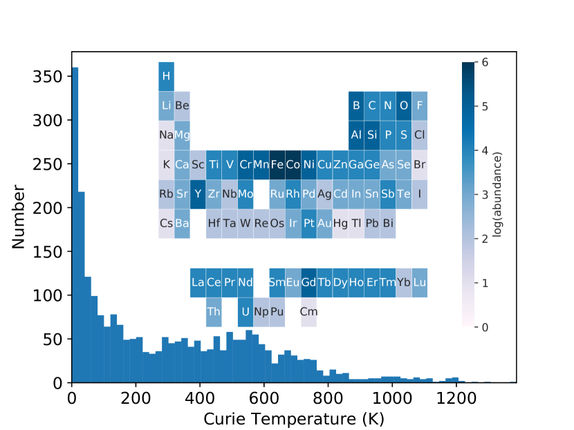
Figure 1: Histogram of the $T_{\mathrm{C}}$’s of about 2,000 known ferromagnets. The median value of the distribution is 227 K. The insert shows the relative elemental abundance, in logarithmic scale, for the ferromagnets included in the dataset (the logarithm of the number of compounds containing a particular element). The most frequent magnetic element is Co followed by Fe and Gd.

Figure 1 also presents the relative elemental abundance for the ferromagnets included in the dataset, namely for every element the number of compounds that contain that given element. As expected the vast majority of the ferromagnets contains at least one of the 3$d$ magnetic transition metals, Fe, Co, Ni and Mn, with Al being the most frequent of the non-magnetic ions. However, it is interesting to note that, with the only exception of noble gases and highly radioactive elements, magnets can be made by incorporating essentially any ion in the periodic table. This gives us a potentially very large chemical space to explore when designing new magnets.

In the last few years there have been a few attempts at systematically predicting the existence of new magnets ahead of experiments. These study are typically based on high-throughput numerical explorations Curtarolo et al. (2013), where the electronic structure of hypothetical compounds is computed at the level of density functional theory. The construction of the prototypes to calculate usually proceeds by substituting elements in known phases Möller et al. (2018); Körner et al. (2018), or by exploring the entire chemical space compatible with a given crystal structure Sanvito et al. (2017). In both cases one can extract some elementary magnetic properties of the prototypes (magnetic moment per cell, density of states, magneto-crystalline anisotropy, etc.) and possibly assess their thermodynamical stability, namely one can forecast if a given prototype can be made and what its magnetic properties would be.

However, little information about $T_{\mathrm{C}}$ can be extracted, unless the specific class of compounds investigated satisfies some simple empirical rules. For example the Curie temperature of Heusler alloys of composition Co${}_{2}XY$, with $X$ and $Y$ being either a transition metal or a main group element, follows a Slater-Pauling curve Graf et al. (2011a), while Mn-containing magnets can be arranged along the phenomenological Castelliz-Kanomata curves Castelliz (1955); Kanomata et al. (1987). In the absence of such empirical rules the search for new compounds remains blind to $T_{\mathrm{C}}$. This is a rather severe deficiency, since the calculations cannot distinguish from the outset which regions of the chemical space may yield high-$T_{\mathrm{C}}$ magnets. As a consequence most of the discovery computational effort is usually spent for materials with little technological potential.

Note that the prediction of $T_{\mathrm{C}}$ by first-principle methods is not an easy task either. The most common strategy consists in mapping electronic structure calculations onto some effective Hamiltonian, most typically the Heisenberg model, which is then used to extract $T_{\mathrm{C}}$ via Monte Carlo techniques. This is a valid approach only if the relevant part of the magnetic excitation spectrum has a spin-wave nature, which is not universally guaranteed. As such the same method applied to different materials may result in predictions of $T_{\mathrm{C}}$’s with a very different level of agreement to experiments Turek et al. (2006). Certainly, the computation of the entire magnetic excitation spectrum with density functional theory is possible Buczek et al. (2009), but the computational overheads are significant. Furthermore, also in this case uncertainty and errors arise from the choice of the exchange and correlation functional and from the other approximations taken. Overall, first-principle methods are very valuable for understanding the origin of a particular $T_{\mathrm{C}}$, but they are currently not fit to be used as a prediction tool ahead of experiments. For all these reasons it would be desirable to construct a universal predictor for $T_{\mathrm{C}}$ based solely on chemical information.

The present work responds to this demand. We introduce a range of machine-learning (ML) models, uniquely based on known experimental data for about 2,500 ferromagnets, which can predict the Curie temperature using only chemical information. Machine learning is rapidly becoming a valuable tool in physics and materials science and it has been used already for a relatively wide range of problems. These go from the accelerated discovery of new materials Pilania et al. (2013); Meredig et al. (2014), to the estimation of materials physical quantities Rupp et al. (2012); Isayev et al. (2017), to the definition of novel density functionals Snyder et al. (2012); Nelson et al. (2019). Here we use ML to unveil patterns in the chemical-to-$T_{\mathrm{C}}$ relation, and use these patterns as predictors for the $T_{\mathrm{C}}$ of new materials. Our approach is in the same spirit of that used by Stanev and co-workers Stanev et al. (2018) to sort superconductors according to their critical temperature.

Our paper is structured as follows. Firstly, we introduce the computational methods used. In particular we discuss extensively the issues of representing the chemical composition of a given compound, of creating and processing the dataset, and of training and choosing the most appropriate and best performing ML model. We then discuss the performance of the various models against our dataset and show their ability to extrapolate in regions of data, where little information were available during the model training. These, for instance, include the prediction of $T_{\mathrm{C}}$ along the composition space of different transition-metal binary systems and for the Al-Co-Fe ternary one. Finally we outline some possible ways to include information about the materials structure in the ML model and its effect on the overall accuracy.

II Methods

II.1 Definition of the feature vectors

The goal of supervised ML is to estimate a function, $f$, that maps a feature vector, x, to a target variable, $y$, namely to find the function $f:\textbf{x}\rightarrow y$ that better interpolates a set of available data (note that the target variable does not need to be a scalar quantity). In our case the feature vector contains information concerning a given compound, while the target variable is $T_{\mathrm{C}}$. Although there are no rigorous stringent rules on how to construct the feature vector, ultimately the success of any ML strategy resides on the ability to define the most relevant features correlating to a given property. When the ML strategy is applied to materials science a number of desirable conditions defining the feature vector emerge naturally Ghiringhelli et al. (2015); Jain et al. (2016); Faber et al. (2015); Rupp et al. (2012); von Lilienfeld et al. (2015). In particular it was proposed that the feature vector

1. should be computationally inexpensive to create.

2. should be continuous, reflecting the fact that the properties of a material vary continuously.

3. should be independent of both the choice of unit cell and of the number of atoms in the unit cell (for periodic solids).

4. should be able to distinguish different materials with different properties, namely different compounds with different $T_{\mathrm{C}}$ should have different feature vectors.

We begin by defining feature vectors that do not include any structural information of compounds, but are constructed to satisfy the first three conditions. Clearly the last one will be automatically violated, since polymorphs of a given chemical composition presenting different $T_{\mathrm{C}}$’s will be described by identical feature vectors. In particular our goal is for the feature vectors to capture the chemical composition of a given compound, namely its chemical formula. We can then divide the features defining a given compound into three categories: features which only take elemental properties into account (e.g. the atomic number), features which take only the compound stoichiometry into account, and features which take both into account.

Notably features belonging to the first category can be found to violate the second criterion and, for this reason, they have been excluded. Take as an example the maximum atomic number, $Z^{\mathrm{max}}$, of a given compound Ward et al. (2016) and consider the binary alloy $\text{A}_{1-x}\text{B}_{x}$, with $Z_{\mathrm{B}}>Z_{\mathrm{A}}$ as an example. At $x=0$ a feature vector containing this component will be discontinuous as the Euclidean distance between $\text{A}_{1}$ and any $\text{A}_{1-x}\text{B}_{x}$ will always be greater than $|Z_{\text{A}}-Z_{\text{B}}|$ and will not go to zero smoothly as $x$ goes to zero. In order to avoid this shortcoming we need to consider features that, either explicitly or implicitly, preserve information related to the atomic fractions of the various elements in a compound, and exclude those that just relate to the elemental properties. As such, features like the number of different elements in the compound (2 for binaries, 3 for ternaries, etc.) or the maximum atomic number are ruled out. In contrast a feature like the mode of the atomic number not is acceptable, since it encodes information about the atomic fractions.

Possible features created solely from the stoichiometry of a compound include the $L^{p}$ stoichiometry norm Ward et al. (2016) and the stoichiometry entropy. The first one is generally defined as $||x||_{p}=(\sum_{i}|x_{i}|^{p})^{1/p}$, while the second is $S=-\sum_{i}x_{i}\log(x_{i})$, where $x_{i}$ is the atomic fraction of the i-$th$ element. Features based on the product of the atomic fractions or on the number of different elements in the compound are ruled out by the second principle, using arguments similar to the one given above. In any case, one has still to establish whether stoichiometry-only features are informative enough for predicting most quantities.

Finally there are generally two ways to define features that take both elemental properties and stoichiometry into account. One possibility is to associate to each compound a high-dimension vector defined as

$$\mathbf{v}_{\mathrm{chem}}=\{x_{\mathrm{H}},x_{\mathrm{He}},x_{\mathrm{Li}},x_{\mathrm{Be}},...\}$$ (1)

where $x_{\alpha}$ is the atomic fraction of element $\alpha$. For instance, $\text{Fe}_{3}\text{O}_{4}$ is represented as the vector $(...,0,4/7,0,...,0,3/7,0...)$, with 4/7 assigned at the eighth position (oxygen) and 3/7 to the 26th one (iron). The advantage of $\mathbf{v}_{\mathrm{chem}}$ is that it uniquely represents a chemical formula, and its disadvantage that the vectors tend to be very sparse and high dimensional, hence difficult to train. A second option was suggested by Ward et al. Ward et al. (2016) and consists in using composition-weighted elemental-properties. An example of these is the composition-weighted atomic number, defined as $\langle Z\rangle=\sum_{i}Z_{i}x_{i}$, with $Z_{i}$ and $x_{i}$ being the atomic number and the atomic fraction of the element $i$. In the case of $\text{Fe}_{3}\text{O}_{4}$ this is $8(4/7)+26(3/7)=15.71$. Similar quantities can be constructed with analogous definitions. Furthermore, for any elemental quantity $Q$ one can also define a composition-weighted mode $\langle|Q|\rangle$, which takes the $Q$ value of the element with the highest atomic fraction in the compound and an average in the case of multiple modes, and a composition-weighted absolute deviation $\langle\Delta Q\rangle=\sum_{i}|Q_{i}-\langle Q\rangle|x_{i}$. Table 1 summarises the features used in this work.

Features	Symbol	Dim.
$L^{p}$ stoichiometry norm ($p=1,2,3$)	$||x||_{p}$	3
Stoichiometry entropy	$S$	1
Atomic fraction vector	$\mathbf{v}_{\mathrm{chem}}$	84
CW atomic number	$\langle Z\rangle$, $\langle|Z|\rangle$, $\langle\Delta Z\rangle$	3
CW valence electrons	$\langle N_{\mathrm{V}}\rangle$, $\langle|N_{\mathrm{V}}|\rangle$, $\langle\Delta N_{\mathrm{V}}\rangle$	3
CW period	$\langle P\rangle$, $\langle|P|\rangle$, $\langle\Delta P\rangle$	3
CW group	$\langle G\rangle$, $\langle|G|\rangle$, $\langle\Delta G\rangle$	3
CW molar volume	$\langle V\rangle$, $\langle|V|\rangle$, $\langle\Delta V\rangle$	3
CW melting $T$	$\langle T_{\mathrm{M}}\rangle$, $\langle|T_{\mathrm{M}}|\rangle$, $\langle\Delta T_{\mathrm{M}}\rangle$	3
CW electronegativity	$\langle\epsilon\rangle$, $\langle|\epsilon|\rangle$, $\langle\Delta\epsilon\rangle$	3

Table 1: The full list of features used in this work. In the last column we report the dimension of any given feature. The atomic fraction vector has dimension 84, as not all elements in the periodic table can be found in the ferromagnets included in our database (e.g. He, Ar, etc.). In total our feature vector has a dimension of 129. Here “CW” denotes “composition-weighted”. The numerical values of the elemental properties are taken from Ref. Ong et al. (2013).

II.2 Machine-learning models training

In an ideal situation, where there is abundance of data, the training of ML models proceeds by splitting the dataset into three mutually exclusive partitions, a training set, a validation set and a test set Friedman et al. (2009). The training set is used to train the model. Most ML models are defined by one or more parameters, called hyperparameters, which cannot be learnt from the data and thus need to be specified from the outset. The validation set is then used for determining the best hyperparameters of any given model and for choosing the best overall model. Finally, the test set is used for estimating the generalization error of the model, namely for assessing how well the given model performs on never-seen-before data. However, in situations where the datasets are small, splitting the data into three sets makes each one of them too small, diminishing the overall ability of the model to learn and hence its accuracy. Therefore, in this case the training and the validation sets are combined into a single set, which we will refer to henceforth as the training set. Then $K$-fold cross-validation is used to determine the hyperparameters and to select the best model. Here the training set is split into $K$ subsets (in this work $K$ was chosen to be $K=3$). For each given set the model is trained over the other $K-1$ sets and tested over the remaining one, the cross-validation error is the average of all the errors. Then the best model, namely the model with the lowest cross-validation error, is trained over the entire training set. Finally, the test set is used to estimate the accuracy of the chosen model.

In order to quantify the model’s performance we have used the coefficient of determination, $R^{2}$. Given a set of target variables $\{y^{i}\}$, with mean $\mu$ and predicted values $\{f(\textbf{x}^{i})\}$, $R^{2}$ is given by

$$R^{2}=1-\frac{\sum_{i}[y^{i}-f(\textbf{x}^{i})]^{2}}{\sum_{i}[y^{i}-\mu]^{2}}\>.$$ (2)

A perfect predictor of the target variables would always score $R^{2}=1$ on any set [$f(\textbf{x}^{i})=y^{i}$ for $\forall i$].

II.3 Construction of the dataset

The dataset of experimental $T_{\mathrm{C}}$ has been constructed by aggregating the following sources: the AtomWork database Xu et al. (2011), Springer Materials Connolly (2012), the Handbook of Magnetic Materials Buschow and Wohlfarth (2009) and the book Magnetism and Magnetic Materials Coey (2010). A few additional values have been taken from the references Albert and Rubin (1971); Givord and Lemaire (1971); Okamoto (1989). For a number of compounds the various databases report multiple values of $T_{\mathrm{C}}$, and there are also compounds where the same database returns a range of $T_{\mathrm{C}}$’s for the same ferromagnet. Notably in the vast majority of cases the spread of $T_{\mathrm{C}}$’s about the mean is rather small, so that the choice of a particular value is irrelevant. In particular, for 79% of the compounds associated to multiple $T_{\mathrm{C}}$’s the difference between the maximum and minimum value is less than 50 K. However, there is also a number of compounds presenting a much larger range of reported critical temperatures, namely for 4.9% of the multiple-$T_{\mathrm{C}}$ data the difference between the maximum and minimum $T_{\mathrm{C}}$ value is greater than 300 K.

There are several reason for these occurrences. In some compounds magnetism is subtly related to the quality of the sample, so that experiments performed by different groups may report different $T_{\mathrm{C}}$. This is particularly relevant, since the various data sources contain $T_{\mathrm{C}}$’s extracted over different periods of time, so that the spread of data sometime reflects the improvements in crystal growth over time. A second reason is related to polymorphism, namely to the existence of compounds with the same stoichiometry but different crystal structure, and hence different $T_{\mathrm{C}}$. Finally, there are several transition-metal/rare-earth intermetallic magnets for which multiple $T_{\mathrm{C}}$ are reported. For instance the two values of 186 K Carfagna and Wallace (1968) and 641 K Buschow (1977) have been both reported for $\text{Sm}_{2}\text{Ni}_{17}$. Such large discrepancy has been attributed to the presence of possible secondary phases Buschow (1977). Since we are aiming at constructing ML models that use only chemical information to define compounds, our feature vector can not include any attribute related to sample quality or polymorphism. As such, in the presence of multiple $T_{\mathrm{C}}$’s we have to establish a criterion to select a single value for any stoichiometry. In this work we have used the median of the distribution instead of the mean or the maximum value as this is more resistant to outliers. For instance, if for a given compound the reported $T_{\mathrm{C}}$’s are 300 K, 305 K and 700 K, their mean is 435 K while their median is 305 K. The first one is not associated to any real measurement while the second is.

In preparing our dataset we have carefully checked that there is enough diversity in the entries. Consider the following thought experiment. Suppose that for every entry in our database there are also many similar entries, namely there are several compounds with similar stoichiometry (feature vector) and similar $T_{\mathrm{C}}$. This may be, for instance, the case of a binary alloy $A_{x}B_{1-x}$, where many data are available in a narrow range of compositions. For a dataset of such homogeneous composition it is likely that almost any ML model will perform well. However, the same model will be unlikely to perform well for compounds significantly different to the ones found in the training set, namely the model will have little ability to generalize to a broader composition range. This is, of course, an unwanted feature. Our strategy to curate the database is then the following. Firstly, we standardise the chemical formula notation, by replacing fractional stoichiometry with integer one (e.g. Cu_0.5Ni_0.5 becomes CuNi = Cu₁Ni₁), and by simplify the stoichiometry when possible (e.g. Ni₇₅Al₂₅ becomes Ni₃Al = Ni₃Al₁). At this point we check for duplicates and, if these result in multiple $T_{\mathrm{C}}$’s for the same stoichiometry we take the median value. Next the dataset is ordered according to the number of atoms in the chemical formula and we compute the $L^{1}$-norm of the atomic fraction vector, $\mathbf{v}_{\mathrm{chem}}$, between all the entries in the database. If the distance between two entries is less than 0.01 we remove the compound with the larger number of atoms in its chemical formula. The rational for doing this reflects our intuition that Fe₅Sn₃ and Fe₈Sn₅, with a distance of 0.019, should be considered as two different compounds, while Co₅Tb₁ and Co_5.1Tb₁, with a distance of 0.005, are essentially the same compound. In this last case we keep only the simpler Co₅Tb₁.

Finally our data needs to enable the ML models to distinguish between magnetic and non-magnetic materials. This is not an issue if our only goal is that of describing the $T_{\mathrm{C}}$ of known ferromagnets, but it becomes one when the ML model is used as $T_{\mathrm{C}}$ predictor for unknown, hypothetical, compounds. As constructed, our data distribution, $p_{\text{data}}$, only includes ferromagnets, so that a ML model will not be able to learn from $p_{\text{data}}$ about stoichiometries having $T_{\mathrm{C}}=0$. A possible way out, as suggested by Stanev et al. Stanev et al. (2018), is that of first training a classifier to predict whether or not a given compound has a $T_{\mathrm{C}}$ greater than some critical value, $T_{\text{critical}}$. If one sets $T_{\text{critical}}$ relatively low, the classifier will distinguish between magnetic compounds and magnetic only at very low temperature. Here, however, we take a somewhat more straightforward approach and we simply include in our dataset some non-magnetic materials. In particular we include the elemental phases of all the non-magnetic elements of the periodic table. This procedure effectively provides to the ML model some information about non-ferromagnets and hopefully it makes it more robust when making new predictions.

After the data processing described above our training set contains 1,866 entries, while the test set has 767. About 3% of the compounds are unaries, including the non-ferromagnetic ones. The ferromagnetic elemental phases are: Co ($T_{\mathrm{C}}=1380$ K), Fe (1040 K), Ni (630 K), Gd (290 K), Tb (220 K), Dy (85 K), Nd (30 K), Tm (30 K), Er (20 K), Ho (20 K) and Pr (8.7 K). Binaries and ternaries make up 31% and 49% of the dataset respectively with the rest of the dataset having more than 3 distinct elements.

III Results

III.1 Machine-learning model performance

In the construction of the ML models we compare four different algorithms, namely Ridge Regression (Ridge), Neural Network (NN), Kernel Ridge Regression (KRR) and Random Forests (RF). The NN is implemented employing Keras Chollet et al. (2015), while for the rest we use Scikit-Learn Pedregosa et al. (2011). For both Ridge and KRR the cross-validation set is used to determine the optimum regularization parameter. In contrast the dropout rate is the hyper-parameter used for the NN, while the maximum depth of the tree is that for RF. The accuracy of many algorithms can be sometimes improved by reducing the dimension of the feature space. This is particularly true when there is correlation between the various features and for ML algorithms affected by the curse of dimensionality Bellman (1957). For a feature vector of dimension $p$, one can construct $2^{p}$ possible subsets of the features, which in our case translates in $\sim 10^{39}$ subsets Not . It is, therefore, infeasible to perform an exhaustive search for the best performing subset. Instead, we have decided to use two different methods of feature-dimension reduction, namely Correlation (C) and Principle Component Analysis (PCA), and used such methods together with all the chosen ML algorithms. Correlation ranks the features according to the absolute value of the Pearson correlation coefficient, which is defined as $c_{\mathrm{P}}=\text{cov}(x,y)/\sigma_{x}\sigma_{y}$, with cov$(x,y)$ being the $(x,y)$ covariance and $\sigma$ the standard deviation. In our case $y$ is the $T_{\mathrm{C}}$ and $x$ corresponds to each feature. In contrast, the PCA projects the feature space into a lower dimensional one, while trying to preserve as much data variance as possible Goodfellow et al. (2016).

The results of the 3-fold cross validation score for the different algorithms operated together with different feature reduction techniques are shown in Table 2.

$R^{2}$	All	C10	C20	C40	C80	P10	P20	P40	P80
Ridge	0.53	0.48	0.5	0.52	0.52	0.24	0.27	0.31	0.39
KRR	0.69	0.72	0.72	0.72	0.69	0.69	0.72	0.70	0.68
NN	0.76	0.72	0.76	0.77	0.78	0.73	0.77	0.77	0.77
RF	0.81	0.76	0.77	0.78	0.79	0.72	0.74	0.73	0.72

Table 2: 3-fold cross-validation $R^{2}$ score of all the algorithms chosen combined with the various feature reduction techniques. “All” indicates the case where no feature reduction is applied. “C” means Correlation feature reduction and “P” is for PCA. The number beside the type of feature reduction scheme indicates the size of the reduced feature space. Thus, for example, P40 means that PCA has generated a 40-dimensional feature space.

In general we find that the performance of the different algorithms ranks them in the following order Ridge, KRR, NN and RF. Dimensionality reduction does not seem to significantly improve the $R^{2}$ and in fact, with the only exception of the Correlation scheme applied to KRR and NN, it appears always better to run the ML algorithm over the full feature space. Overall Random Forests using the entire set of features performs the best on the cross-validation sets and, therefore, it is chosen as the final model. RF achieves a cross-validation $R^{2}$ of 0.81 and a test one of 0.87, demonstrating that the cross-validation score is a good estimate of the test error.

In Fig. 2 we present our best result for the RF algorithm. Here we plot the predicted $T_{\mathrm{C}}$’s against the experimental ones for all the ferromagnets contained in the test set. In addition we present a distribution of the absolute errors and one for the relative error of compounds presenting $T_{\mathrm{C}}>300$ K. In general we find that our ML model can predict relatively well the experimental $T_{\mathrm{C}}$, in particular for Curie temperatures exceeding 300 K. This is important since in this range one finds the magnets useful for room-temperature applications. The mean absolute error over the entire distribution is 57 K. Such a value gives us confidence that the ML model can distinguish between high-$T_{\mathrm{C}}$ ferromagnets and low-$T_{\mathrm{C}}$ ones, namely it allows us to identify the potential of an hypothetical chemical composition against ferromagnetism.

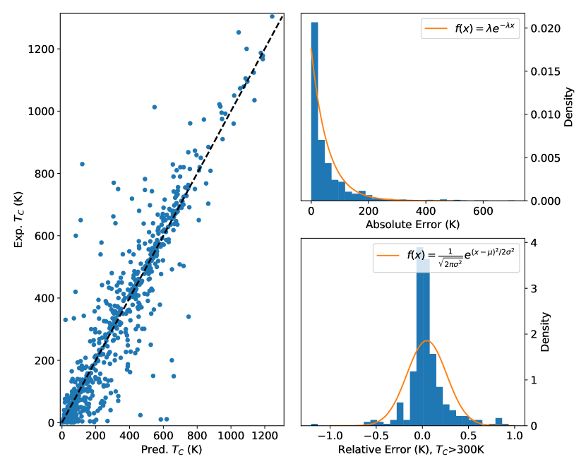
Figure 2: RF model for the $T_{\mathrm{C}}$ of ferromagnets. In the left-hand side panel we compare the experimental and predicted $T_{\mathrm{C}}$ for the test set. The $R^{2}$ coefficient of the model is 0.87 and the mean absolute value is 57 K. The upper left panel shows the distribution of absolute errors, $|T_{\mathrm{C}}^{\mathrm{exp}}-T_{\mathrm{C}}^{\mathrm{predic}}|$, while the lower one displays the distribution of the relative errors for compounds with $T_{\mathrm{C}}>300$ K. The orange lines indicate the best fit respectively to an exponential and a Gaussian distribution.

The distribution of the $T_{\mathrm{C}}$ absolute errors for our best ML model is exponential with decay coefficient, $\lambda$, of 0.018. From the distribution one can learn that an $1-e^{-\lambda x}$ fraction of the data are with $x$ K of the experimental data. For example 59 % of the predicted $T_{\mathrm{C}}$’s are within 50 K from the measured ones, and 83 % are within 100 K. Large absolute errors are found only for compounds presenting a rather small $T_{\mathrm{C}}$, which are erroneously predicted to be robust ferromagnets. A more detailed understanding of the performance of our ML model can be obtained by looking at the distribution of the relative error, defined as $(T_{\mathrm{C}}^{\mathrm{exp}}-T_{\mathrm{C}}^{\mathrm{predic}})/T_{\mathrm{C}}^{\mathrm{exp}}$, where $T_{\mathrm{C}}^{\mathrm{exp}}$ and $T_{\mathrm{C}}^{\mathrm{predic}}$ are respectively the average experimental $T_{\mathrm{C}}$ and the predicted one. In this case we present data only for compounds with $T_{\mathrm{C}}$ exceeding 300 K (right-hand side panel of Fig. 2). There are two main reasons behind such choice. On the one hand, these are the compounds potentially useful for room-temperature applications. On the other hand, for ferromagnets presenting low measured $T_{\mathrm{C}}$, relative small absolute errors may result in rather large relative ones. In this case the distribution appears symmetric around zero, indicating that our ML model has no systematic bias towards either overestimating or underestimating $T_{\mathrm{C}}$. The shape of the distribution is Gaussian-type with a half-height width of 0.51. We find that only 5 % of the compounds present a relative error larger than 50 %, and only 15 % have errors larger than 25 %.

Finally we take a look at whether or not our ML model tends to systematically fail for some particular chemical compositions. Again we analyse data only for compounds with $T_{\mathrm{C}}>300$ K. In Table 3 we present the elemental abundance, $f_{M}^{\alpha}$, of the most relevant magnetic transition metals, $M$, among compounds presenting a relative error beyond a give threshold, $\alpha$. For instance, in the cell corresponding to $f^{50}_{M}$ and Cr we show the relative abundance of the Cr element among the compounds presenting a predicted $T_{\mathrm{C}}$ with a relative error larger than 50 %, $f^{50}_{\mathrm{Cr}}$. The abundance is calculated as the total number of compounds presenting a given element divided by the total number of compounds. Note that the elemental abundances do not necessarily sum up to unity, since a compound may contain more than one transition metal.

Element	$f_{M}^{50}$	$f_{M}^{30}$	$f_{M}^{20}$	$f_{M}^{10}$	$f_{M}^{5}$	$f_{M}^{2}$	$f_{M}^{0}$
Cr	0.0	0.01	0.02	0.02	0.04	0.05	0.05
Mn	0.02	0.04	0.08	0.09	0.12	0.14	0.15
Fe	0.03	0.07	0.13	0.24	0.38	0.56	0.74
Co	0.01	0.02	0.03	0.06	0.11	0.17	0.21
Ni	0.01	0.02	0.02	0.03	0.04	0.05	0.05
Total	0.05	0.13	0.21	0.36	0.56	0.79	1.0

Table 3: Elemental abundance, $f_{M}^{\alpha}$, of the most relevant magnetic transition metals, $M$, among compounds presenting a relative error beyond a give threshold, $\alpha$ (in %). The last row, labelled as ‘total’, lists the fraction of compounds with errors exceeding $\alpha$ (e.g. 0.13 of the compounds have a predicted $T_{\mathrm{C}}$ with error exceeding 30%). The last column (error 0 %) shows the elemental abundance over the entire set.

In general, as expected, we find that the elemental abundance grows as the error on the predicted $T_{\mathrm{C}}$ gets smaller. Such dependence is rather flat for Cr, Mn and Ni, mostly because a relatively limited number of compounds containing these three transition metals are found ferromagnetic above 300 K. The distribution of errors is thus dominated by Fe-containing, and partially Co-containing, ferromagnets, which are calculated with an accuracy comparable to that of the total set. We can then conclude that our best ML model is well balanced across chemical composition and does not favour any particular region of the chemical space.

III.2 Ability of the model to extrapolate

Next we demonstrate the ability of our model to extrapolate to regions of the chemical space where only a few data points were present in the training set. Our first example consists in predicting the $T_{\mathrm{C}}$ as a function of composition for three binary systems. In particular we consider Co-Mn, Fe-Ni and Ni-Rh for concentration ranges where the alloys remain ferromagnetic. Our results are presented in Fig. 3, where we show the prediction of our ML model against available experimental data. In particular we distinguish between the data included in the training set (black crosses) and those that they were not (green dots). Using the Random Forest algorithm we can measure the models uncertainty by looking at the distribution of the predictions of the individual trees. In practice, we measure the uncertainty by grouping the trees into subsets of five trees each, averaging over these subsets and then using the minimum and maximum average as our uncertainty boundaries. In the test set 82 % of the experimental values were within 50 K of the confidence interval. In the figure for every composition we present the average predicted $T_{\mathrm{C}}$ (blue line) and also the confidence interval of the random forest algorithm (light-blue shadow).

Figure 3: $T_{\mathrm{C}}$ prediction as a function of composition for three binary transition-metal systems, namely Co-Mn, Fe-Ni and Ni-Rh. Data are presented as a function of the atomic fraction of one of the two species. The blue line traces the ML prediction, black crosses (green dots) are experimental points included (not included) in the training set. The experimental results are taken from references Menshikov et al. (1985); Swartzendruber et al. (1991); Crangle and Parsons (1960). The light-blue shadowed area corresponds to the range of predicted $T_{\mathrm{C}}$’s of subsets of the trees, namely it indicates the uncertainty of the ML model. In the middle panel the red dots correspond to the $T_{\mathrm{C}}$ associated to the FeNi₃ intermetallic phase, while the green ones correspond to random Ni-Fe alloys.

Manganese and cobalt can form disordered alloys with a few possible crystal structures across the entire composition range Ishida and Nishizawa (1990). The magnetic phase diagram was determined sometime ago Menshikov et al. (1985) and comprises both ferromagnetic and antiferromagnetic orders. In particular when the Co atomic fraction is larger than about 0.68 the alloys are ferromagnetic with a $T_{\mathrm{C}}$ that monotonically increases as a function of the Co content. In contrast, Mn-rich alloys are antiferromagnetic with a Néel temperature that this time monotonically increases as the Mn concentration gets larger. Our ML model predicts well the $T_{\mathrm{C}}$ for all the ferromagnetic phases, with a constant minimal error. For this case only two data points were included in the training set, namely elemental Co and the end-of-the-series alloy, Co₁₃Mn₇. Intriguingly, the model seems to be able to predict also the upturn in critical temperature occurring for Co atomic fractions lower than 0.68, although these correspond to antiferromagnetic phases. It is worth noting that the spread of values returned by the RF algorithm is certainly larger for these Mn-rich phases.

The Ni-Fe system presents a different level of complexity, with the ferromagnetic order being present over the entire composition range Swartzendruber et al. (1991). In the region of temperatures relevant for $T_{\mathrm{C}}$ the Fe-rich phases (for a Fe atomic fraction down to 0.65) are characterized by Ni-doped bcc iron with a $T_{\mathrm{C}}$ that grows monotonically as a function of the Fe fraction. In contrast, when the Fe atomic fraction is reduced below 0.65 the relevant phase is an fcc random alloy, which can be stabilized up to bulk Ni. In this case the $T_{\mathrm{C}}$ is non-monotonic, it increases with the Ni atomic fraction up to 0.70 (the maximum $T_{\mathrm{C}}$ is about 870 K for Fe₃₀Ni₇₀) and then it decreases down to the $T_{\mathrm{C}}$ of bulk Ni. Furthermore, there is also an ordered intermetallic FeNi₃ ferromagnetic phase, which persists over a relatively narrow composition range. This means that in Fe_1-xNi_x at $x\sim 0.75$ there are two ferromagnetic phases with different $T_{\mathrm{C}}$’s. Also in this case our ML model performs rather well. This time seven experimental data points were included in the training set, two for the elemental Ni and Fe and five across the Fe_1-xNi_x alloys. In particular the composition corresponding to the maximum at the intermetallic FeNi₃ phase was included. Our ML model interpolates well between these points, in particular in the Ni-rich part of the composition diagram. As expected from the fact that structural information are not included in the model, we are not able to distinguish the different $T_{\mathrm{C}}$’s associated to different structures.

Finally, we look at the Ni-Rh binary system, an alloy where only one of the two elements is magnetic. As with several other elements of the Pt group, Rh is highly soluble in Ni and random alloys can be formed over almost the entire composition range. Here the $T_{\mathrm{C}}$ monotonically decreases from that of bulk Ni as Rh is added to the alloy. This continues up to a critical composition, found for a Ni atomic fraction of around 63%, where the ferromagnetism disappears completely Muellner and Kouvel (1975). Our ML model is fully capable of describing such behaviour. In particular the ML model successfully predicts the critical concentration for the suppression of ferromagnetism at a Ni atomic fraction lower then 0.7. This is a rather compelling result.

As a second example of the ability of our ML model to extrapolate to unexplored regions of the chemical space we present the $T_{\mathrm{C}}$ diagram of the ternary system Al-Co-Fe.

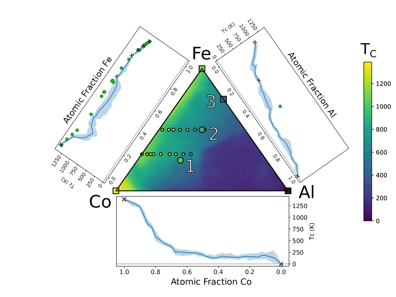
Figure 4: $T_{\mathrm{C}}$ prediction as a function of composition for the ternary system Al-Co-Fe. Data are presented as a function of the atomic fraction of the three species and the $T_{\mathrm{C}}$ is expressed as a heat map. The figure also introduces a detailed analysis of the three relevant binary phase diagrams, where the blue line traces the ML prediction, black crosses (green dots) are experimental points included (not included) in the training set. The light-blue shadowed area in the binary plots corresponds to the range of predicted $T_{\mathrm{C}}$’s, namely it indicates the uncertainty of the ML model. The solid square (circles) included in the ternary $T_{\mathrm{C}}$ diagram are for experimental data included (not included) in the training set, with the colour code describing the $T_{\mathrm{C}}$. Numbers correspond to three known stoichiometric phases: 1) Co₂FeAl, $T_{\mathrm{C}}=$ 1,000 K, 2) Fe₂CoAl, $T_{\mathrm{C}}>$ 873 K, 3) Fe₃Al, $T_{\mathrm{C}}=$ 573 K. The plot was partially made using python-ternary Harper et al. (2015).

In Fig. 4 we show the $T_{\mathrm{C}}$ across the ternary composition space as a colour-coded heat map and that across the three possible binary systems as a standard graph, similar to those of Fig. 3. Also in this case for the binary systems we represent the data included in the training set as black crosses and those outside the training set as solid dots. The same convention is adopted for phases in the middle of the ternary diagram, where now the data included in the training set are solid square. Note that this ternary system includes three stoichiometric magnetic phases, namely Co₂FeAl Graf et al. (2011b), Fe₂CoAl Yin et al. (2015) and Fe₃Al Nathans et al. (1958). Furthermore, magnetic solid state solutions can be stabilized over a rather large composition space.

As for the other binary systems investigated (see Fig. 3) our machine learning model appears well able to describe the main features of the three relevant binary alloys, namely Al-Co, Al-Fe and Co-Fe. This is despite the fact that only a rather limited number of compounds across the various phase diagrams were included in our training set. For instance, the model is capable of describing the critical Al concentration for the appearance of ferromagnetism in Al-Co McAlieter (1989), which has been measured to be at an Al atomic fraction of about 50%. In this case only the end points of the composition diagram, namely elemental Co and Al, were present in the training set, so that the ML model is able to extrapolate such critical concentration from the learning obtained in other part of the chemical space.

The case of Al-Fe is relatively more complex. Our ML model is trained with only three data points from this binary system, namely the end points and the Fe₃Al stoichiometric phase. The resulting $T_{\mathrm{C}}$-versus-composition curve then predicts a monotonic reduction of the Curie temperature as the Al atomic fraction increases, with a rather smooth approach to $T_{\mathrm{C}}=0$ for pure Al. Experimental data obtained for rf-sputtered thin films display a well-disordered bcc phase for Al atomic fractions up to 70%, followed by an amorphous phase between 75% and 85%, and then by an fcc phase for higher Al fractions. The disordered bcc phases are all ferromagnetic, while both the amorphous and the fcc ones are paramagnetic down to 4.2 K Shiga et al. (1985). Although the precise position of such phase boundaries seems to depend somewhat on the details of the growth conditions Sumiyama et al. (1990), our ML model appears also in the case to be able to capture such behaviour.

At variance with the Al-Fe and Al-Co case, the $T_{\mathrm{C}}$ of the Co-Fe binary system presents a non-monotonic behaviour with composition. As we move from elemental Co to elemental Fe, first the $T_{\mathrm{C}}$ decreases with increasing the Fe content, up to a Fe atomic fraction of around 30%. In this case the magnetic transition takes place within the Co-Fe $\gamma$-phase (fcc structure). Then, for Fe atomic fractions comprised between $\sim$30% and $\sim$80%, $T_{\mathrm{C}}$ first increases and then decreases, reaching up a maximum at around a 50-50 composition. Such behaviour effectively traces the phase boundary between the $\gamma$ and the $\alpha$ phases (bcc structure). At the end of the composition range, for Fe atomic fractions above 80%, $T_{\mathrm{C}}$ keeps decreasing down to that of elemental Fe, but the alloys remain in the $\alpha$ phase, namely the magnetic phase transition no longer traces the structural phase boundary Nishizawa and Ishida (1984).

Finally, we take a look at the $T_{\mathrm{C}}$’s for the ternary phases, namely in the center of the composition diagram. In this case no experimental information was included in the training set. Two ternary stoichiometry compounds are known for Al-Co-Fe, namely the Heusler alloys Co₂FeAl and Fe₂CoAl. Their Curie temperature are 1,000 K for Co₂FeAl Graf et al. (2011b) and at least 873 K for Fe₂CoAl Yin et al. (2015) ($T_{\mathrm{C}}$ has not been measured with precision and only a lower bound is available). Our ML model predicts respectively 657 K and 580 K, hence it provides an underestimation of the real $T_{\mathrm{C}}$’s, although it ranks the materials in the right order. Additional experimental data are available across the Al-Co composition (for an Al atomic fractions not exceeding 30%) and constant Fe atomic fractions of 30% and 50% Raghavan (2005). These data are reported as full circles in Fig. 4 showing the ability of our ML model to describe the general trend, namely a decrease in $T_{\mathrm{C}}$ as the Al atomic fraction increases. Also in this case some non-monotonicity is found in the experimental data for small Al concentrations, which is associated to the fact that for such composition range the $T_{\mathrm{C}}$ traces the phase boundary between the $\alpha$ and $\gamma$ phases. Our ML model appears to be able to trace such non-monotonicity.

III.3 Incorporating structural information in the feature vector

As constructed, our ML model does not include any information about the atomic structure of a given compound. For this reason it is unable to distinguish the Curie temperatures of two polymorphs having the same chemical composition, a fact that has been discussed in connection to the Ni-rich part of the Fe-Ni $T_{\mathrm{C}}$ diagram (see Fig. 3). We now present an attempt at overcoming such shortfall by including structural information in our feature vector. This is not a trivial task.

Several strategies to encode structural information of materials in a way that satisfies the four criteria introduced in the Method section have been proposed. These include partial radial distribution functions Schütt et al. (2014), Voronoi tessellation Ward et al. (2017) and representations learnt by neural networks Schütt et al. (2018). The issue with including structural information is that it massively increases the size of the input space, thus requiring much more training data to fully capture the space. This may not be a problem when data is abundant or can be easily generated, but it becomes one when the data is limited, as in our case. In fact, out of our entire dataset, only 792 entires have an associated entry in the ICSD database Belsky et al. (2002). As such only this subset of data can be used in a ML model informed by structural parameters.

We have then constructed four different ML models, each one of them containing only a limited description of the structural information of a compound. The first, denoted as Original + Volume, associates to any compound, in addition to the previous features, the unit cell volume per atom. The second one replaces the atomic fraction of each element present in a compound with its volume fraction, defined as $\mathbf{v}_{\mathrm{chem}}\cdot V$, where $V$ is the volume per atom of the material. This is denoted as Original with V-Frac. The next two models, instead, include a more detailed representation of the atomic positions. We have taken inspiration from the work of Schütt et al. Schütt et al. (2014), who introduced structural information in the form of a radial distribution function,

$$f(r)=\frac{1}{N_{\text{cell}}}\sum_{i=1}^{N_{\text{cell}}}\sum_{j}\theta(d_{ij}-r)\theta(r+\Delta-d_{ij})\>.$$ (3)

Here $N_{\text{cell}}$ is the number of atoms in the unit cell, the index $i$ runs over all the atoms in the unit cell, while the index $j$ over all the atoms neighbouring that at $i$ are within some distance cutoff, $\theta(x)$ is the Heaviside step function, $d_{ij}$ is the distance between the atoms $i$ and $j$ and finally $\Delta$ is the interval, a parameter that we must specify. Note that $\theta(d_{ij}-r)\theta(r+\Delta-d_{ij})$ is equal to one if $r<d_{ij}<r+\Delta$ and vanishes otherwise. In our case we evaluate $f(r)$ at the points $r_{n}=n\Delta$, where $n$ is an integer, and the resulting function is added to the original feature vector (Original + f model).

A second strategy, which tries to incorporate more information in the radial distribution function consists in defining an “interaction-resolved radial distribution function”

$$f_{\alpha}(r)=\frac{1}{N_{\text{cell}}}\sum_{i=1}^{N_{\text{cell}}}\sum_{j}\theta(d_{ij}-r)\theta(r+\Delta-d_{ij})\delta_{\alpha,ij}\>.$$ (4)

Here $\alpha$ represents a type of “interaction” and $\delta_{\alpha,ij}$ does not vanish, if the atoms at the positions $i$ and $j$ define that given interaction. In practice, with “TM” meaning a transition metal atom, “LA” a lanthanide, and “OT” an atom of other type, we consider six types of interactions: TM-TM, TM-LA, TM-OT, LA-LA, LA-OT and OT-OT. Thus, the $f_{\alpha}(r)$ radial distribution function effectively defines the type-specific neighbourhood of a given atom. Note that the two distribution functions are related to each other by the sum rule $f(r)=\sum_{\alpha}f_{\alpha}(r)$. The rationale behind $f_{\alpha}$ is that the magnetic exchange interaction is, in general, dependent on the atom type, and determines the $T_{\mathrm{C}}$. As such, by containing the $f_{\alpha}$ our feature vector is expected to have some freedom to learn about the exchange interaction of a given compound. A similar, although more complex, representation was used also by Schütt et al. Schütt et al. (2014). Here we have simplified the description to keep the dimension of the feature vector relatively low. This last model is denoted as Original + $f_{ab}$.

We then use 3-fold cross-validation on the 792-entires data subset with the Random Forests and KRR algorithm, and the results are shown in Table 4. Note first that on this reduced data subset the original feature vector (129-dimensional) is not able to generate ML models as accurate as before. For instance the $R^{2}$ coefficient of the RF algorithm is now only 0.75, compared with the previous value of 0.81. This is expected, since the pool of data used for the construction of the model now has been drastically reduced. Unfortunately, we also find that any additional feature added to the original vector generally makes the construction of an accurate ML model less successful with $R^{2}$ coefficients systematically smaller than those obtained for the original model regardless of the specific ML algorithm used. The exception here is when adding the volume as a feature. However, the improvement is so small that it is doubtful whether this is a significant result. There are two possible reasons, probably both at play, behind this result. Firstly, in all cases the feature vector dimension is larger, while the training dataset is smaller. Thus the models have now less data to train but more information to use, effectively jeopardising their ability to learn. Secondly, we have now little control on the balance of the data, meaning that we may have a disproportionated amount of information across the different regions of the chemical space.

Features	RF $R^{2}$	KRR $R^{2}$	Dim.
Original	0.75	0.64	102
Original + Volume	0.76	0.64	103
Original with V-Frac	0.75	0.61	129
Original + $f$	0.74	0.63	122
Original + $f_{ab}$	0.74	0.64	220

Table 4: The 3-fold cross-validation $R^{2}$ score of the variously defined feature vectors for both Random Forests (RF) and Kernel Ridge Regression (KRR). Note that here “Original” refers to the original set of features. The last column reports the dimension of the feature vector.

IV Conclusion

We have here described the construction of a ML model to predict the Curie temperature of ferromagnets solely based on their chemical composition. The model has been entirely trained over available experimental data and its construction did not involve any electronic structure calculations. We have considered several ML algorithms and, by using Random Forest we have been able to generate a model presenting a mean absolute error of only 57 K over a test set containing 767 compounds. Interestingly most of the error is associated to magnets with low $T_{\mathrm{C}}$, so that the model is capable to identify high-$T_{\mathrm{C}}$ ferromagnets.

We have then made several attempts to include structural information into the description, but we have never been able to outperform the models containing chemical data only. This is likely to be related to the smaller pool of data to use for the training and to the larger dimension of our feature space. It is also interesting to note that ferromagnets, being mostly metallic, are less sensitive than other magnetically ordered compounds to the structural details. All in all our ML model can be viewed as a first rough guide to navigate the chemical space of magnetism, namely as a first step toward a ML-driven magnetic materials discovery strategy.

Acknowledgment

Financial support for this work has been provided by the Irish Research Council. We thanks Alessandro Lunghi for useful discussions and for a critical read of the manuscript.

References

- Coey (2010) J. Coey, Magnetism and magnetic materials (Cambridge University Press, 2010).
- Blundell (2001) S. Blundell, Magnetism in condensed matter (Oxford Univ. Press, 2001).
- Curtarolo et al. (2013) S. Curtarolo, G. L. W. Hart, M. B. Nardelli, N. Mingo, S. Sanvito, and O. Levy, Nature Materials 12, 191 (2013).
- Möller et al. (2018) J. Möller, W. Körner, G. Krugel, D. Urban, and C. Elsässer, Acta Mater. 153, 53 (2018).
- Körner et al. (2018) W. Körner, G. Krugel, D. Urban, and C. Elsässer, Scripta Mater. 154, 295 (2018).
- Sanvito et al. (2017) S. Sanvito, C. Oses, J. Xue, A. Tiwari, M. Zic, T. Archer, P. Tozman, M. Venkatesan, J. Coey, and S. Curtarolo, Sci. Adv. 3, e1602241 (2017).
- Graf et al. (2011a) T. Graf, C. Felser, and S. S. P. Parkin, Prog. Solid State Chem. 39, 1 (2011a).
- Castelliz (1955) L. Castelliz, Z. Metallk. 46, 198 (1955).
- Kanomata et al. (1987) T. Kanomata, K. Shirakawa, and T. Kaneko, J. Magn. Magn. Mater. 65, 76 (1987).
- Turek et al. (2006) I. Turek, J. Kudrnovsky, V. Drchal, and P. Bruno, Phil. Mag. 86, 1713 (2006).
- Buczek et al. (2009) P. Buczek, A. Ernst, P. Bruno, and L. M. Sandratskii, Phys. Rev. Lett. 102, 247206 (2009).
- Pilania et al. (2013) G. Pilania, C. Wang, X. Jiang, S. Rajasekaran, and R. Ramprasad, Sci. Rep. 3, 2810 (2013).
- Meredig et al. (2014) B. Meredig, A. Agrawal, S. Kirklin, J. E. Saal, J. Doak, A. Thompson, K. Zhang, A. Choudhary, and C. Wolverton, Phys. Rev. B 89, 094104 (2014).
- Rupp et al. (2012) M. Rupp, A. Tkatchenko, K.-R. Müller, and O. A. Von Lilienfeld, Phys. Rev. Lett. 108, 058301 (2012).
- Isayev et al. (2017) O. Isayev, C. Oses, C. Toher, S. C. Eric Gossett, and A. Tropsha, Nature Comm. 8, 15679 (2017).
- Snyder et al. (2012) J. C. Snyder, M. Rupp, K. Hansen, K.-R. Müller, and K. Burke, Phys. Rev. Lett. 108, 253002 (2012).
- Nelson et al. (2019) J. Nelson, R. Tiwari, and S. Sanvito, Phys. Rev. B 99, 075132 (2019).
- Stanev et al. (2018) V. Stanev, C. Oses, A. G. Kusne, E. Rodriguez, J. Paglione, S. Curtarolo, and I. Takeuchi, npj Comp. Mat. 4, 29 (2018).
- Ghiringhelli et al. (2015) L. M. Ghiringhelli, J. Vybiral, S. V. Levchenko, C. Draxl, and M. Scheffler, Phys. Rev. Lett. 114, 105503 (2015).
- Jain et al. (2016) A. Jain, G. Hautier, S. P. Ong, and K. Persson, J. Mat. Res. 31, 977 (2016).
- Faber et al. (2015) F. Faber, A. Lindmaa, O. A. von Lilienfeld, and R. Armiento, Int. J. Quant. Chem. 115, 1094 (2015).
- von Lilienfeld et al. (2015) O. A. von Lilienfeld, R. Ramakrishnan, M. Rupp, and A. Knoll, Int. J. Quant. Chem. 115, 1084 (2015).
- Ward et al. (2016) L. Ward, A. Agrawal, A. Choudhary, and C. Wolverton, npj Comp. Mat. 2, 16028 (2016).
- (24) The mode of the atomic number of a compound is defined as the atomic number of the most abundant element of that compound. For example, the atomic number mode of Fe3O4 is 8, the atomic number of oxygen. In case two or more elements have maximal abundance the mode is defined as the average of their atomic numbers.
- Ong et al. (2013) S. P. Ong, W. D. Richards, A. Jain, G. Hautier, M. Kocher, S. Cholia, D. Gunter, V. L. Chevrier, K. A. Persson, and G. Ceder, Comp. Mat. Sci. 68, 314 (2013).
- Friedman et al. (2009) J. Friedman, T. Hastie, and R. Tibshirani, The elements of statistical learning, 2nd ed. (Springer Series in Statistics, 2009).
- Xu et al. (2011) Y. Xu, M. Yamazaki, and P. Villars, Jpn. J. App. Phys. 50, 11RH02 (2011).
- Connolly (2012) T. F. Connolly, Bibliography of magnetic materials and tabulation of magnetic transition temperatures (Springer Science & Business Media, 2012).
- Buschow and Wohlfarth (2009) K. Buschow and E. Wohlfarth, eds., Handbook of Magnetic Materials, Volumes 4-16 & 18 (Elsevier, 1988-2009).
- Albert and Rubin (1971) H. Albert and L. Rubin, Advances in Chemistry series 98, 1 (1971).
- Givord and Lemaire (1971) F. Givord and R. Lemaire, Solid State Commun. 9, 341 (1971).
- Okamoto (1989) H. Okamoto, Bulletin of Alloy Phase Diagrams 10, 549 (1989).
- Carfagna and Wallace (1968) P. D. Carfagna and W. Wallace, J. Appl. Phys. 39, 5259 (1968).
- Buschow (1977) K. Buschow, Rep. Prog. Phys. 40, 1179 (1977).
- Chollet et al. (2015) F. Chollet et al., “Keras,” https://keras.io (2015).
- Pedregosa et al. (2011) F. Pedregosa, G. Varoquaux, A. Gramfort, V. Michel, B. Thirion, O. Grisel, M. Blondel, P. Prettenhofer, R. Weiss, V. Dubourg, J. Vanderplas, A. Passos, D. Cournapeau, M. Brucher, M. Perrot, and E. Duchesnay, J. Mach. Learn. Res. 12, 2825 (2011).
- Bellman (1957) R. Bellman, Dynamic Programming, Rand Corporation research study (Princeton University Press, 1957).
- (38) The value provided here is calculated over all possible feature subsets, regardless of the dimensionality of the associated feature space.
- Goodfellow et al. (2016) I. Goodfellow, Y. Bengio, and A. Courville, Deep learning (MIT press, 2016).
- Menshikov et al. (1985) A. Menshikov, G. Takzei, Y. A. Dorofeev, V. Kazantsev, A. Kostyshin, and I. Sych, Zh. Eksp. Teor. Fiz. 89, 1269 (1985).
- Swartzendruber et al. (1991) L. Swartzendruber, V. Itkin, and C. Alcock, J. Phase Equilib. 12, 288 (1991).
- Crangle and Parsons (1960) J. Crangle and D. Parsons, Proc. R. Soc. London A 255, 509 (1960).
- Ishida and Nishizawa (1990) K. Ishida and T. Nishizawa, Bulletin of Alloy Phase Diagrams 11, 125 (1990).
- Muellner and Kouvel (1975) W. C. Muellner and J. S. Kouvel, Phys. Rev. B 11, 4552 (1975).
- Harper et al. (2015) M. Harper, B. Weinstein, C. Simon, et al., “Python-ternary: ternary plots in python. zenodo,” (2015).
- Graf et al. (2011b) T. Graf, C. Felser, and S. Parkin, Prog. Sol. State Chem. 39, 1 (2011b).
- Yin et al. (2015) M. Yin, P. Nash, and S. Chen, Intermetallics 57, 34 (2015).
- Nathans et al. (1958) R. Nathans, M. Pigott, and C. Shull, J. Phys. Chem. Solids 6, 38 (1958).
- McAlieter (1989) A. McAlieter, Bulletin of Alloy Phase Diagrams 10, 646 (1989).
- Shiga et al. (1985) M. Shiga, T. Kikawa, K. Sumiyama, and Y. Nakamura, J. Magn. Soc. Jpn. Mag. 9, 187 (1985).
- Sumiyama et al. (1990) K. Sumiyama, Y. Hirose, and Y. Nakamura, J. Phys. Soc. Jpn. 59, 2963 (1990).
- Nishizawa and Ishida (1984) T. Nishizawa and K. Ishida, Bulletin of Alloy Phase Diagrams 5, 250 (1984).
- Raghavan (2005) V. Raghavan, J. Phase Equilib. Diff. 26, 57 (2005).
- Schütt et al. (2014) K. Schütt, H. Glawe, F. Brockherde, A. Sanna, K. Müller, and E. Gross, Phys. Rev. B 89, 205118 (2014).
- Ward et al. (2017) L. Ward, R. Liu, A. Krishna, V. I. Hegde, A. Agrawal, A. Choudhary, and C. Wolverton, Phys. Rev. B 96, 024104 (2017).
- Schütt et al. (2018) K. T. Schütt, H. E. Sauceda, P.-J. Kindermans, A. Tkatchenko, and K.-R. Müller, J. Chem. Phys. 148, 241722 (2018).
- Belsky et al. (2002) A. Belsky, M. Hellenbrandt, V. Karen, and P. Luksch, Acta Cryst. B 58, 364 (2002).