Non-LTE analysis of K I in late-type stars

Abstract

Context. Older models of Galactic chemical evolution (GCE) predict [K/Fe] ratios as much as $1\,\mathrm{dex}$ lower than those inferred from stellar observations. Abundances of potassium are mainly based on analyses of the $7698\ \AA$ resonance line, and the discrepancy between GCE models and observations is in part caused by the assumption of local thermodynamic equilibrium (LTE) in spectroscopic analyses.

Aims. We study the statistical equilibrium of K I, focusing on the non-LTE effects on the $7698\ \AA$ line. We aim to determine how non-LTE abundances of potassium can improve the analysis of its chemical evolution, and help to constrain the yields of GCE models.

Methods. We construct a new model K I atom that employs the most up-to-date atomic data. In particular, we calculate and present inelastic e+K collisional excitation cross-sections from the convergent close-coupling (CCC) and the $B$-Spline $R$-matrix (BSR) methods, and H+K collisions from the two-electron model (LCAO). We constructed a fine, extended grid of non-LTE abundance corrections based on 1D MARCS models that span $4000<T_{\mathrm{eff}}/\rm{K}<8000$, $0.50<\log{g}<5.00$, $-5.00<\mathrm{\left[Fe/H\right]}<+0.50$, and applied the corrections to potassium abundances extracted from the literature.

Results. In concordance with previous studies, we find severe non-LTE effects in the $7698\ \AA$ line. The line is stronger in non-LTE and the abundance corrections can reach $\sim-0.7\,\mathrm{dex}$ for solar-metallicity stars such as Procyon. We determine potassium abundances in six benchmark stars, and obtain consistent results from different optical lines. We explore the effects of atmospheric inhomogeneity by computing for the first time a full 3D non-LTE stellar spectrum of K I lines for a test star. We find that 3D modeling is necessary to predict a correct shape of the resonance 7698Å line, but the line strength is similar to that found in 1D non-LTE.

Conclusions. Our non-LTE abundance corrections reduce the scatter and change the cosmic trends of literature potassium abundances. In the regime [Fe/H]$\lesssim-1.0$ the non-LTE abundances show a good agreement with the GCE model with yields from rotating massive stars. The reduced scatter of the non-LTE corrected abundances of a sample of solar twins shows that line-by-line differential analysis techniques cannot fully compensate for systematic LTE modelling errors; the scatter introduced by such errors introduces a spurious dispersion to K evolution.

1 Introduction

Potassium is an alkali metal with an atomic structure very similar to that of sodium (so similar that they were mistakenly believed to be the same element until after the eighteenth century). However, K is typically an order-of-magnitude less abundant than Na and its spectral fingerprint in late-type stars is accordingly weaker and much less studied. Potassium has three stable isotopes (³⁹K, ⁴⁰K and ⁴¹K); all produced via hydrostatic oxygen shell burning and explosive oxygen burning in massive stars, with a relative proportion that depends on the stellar mass (Woosley & Weaver, 1995). The lightest isotope is dominant with 93% occurrence in solar-system meteorites (Lodders & Palme, 2009). Because of this, and the negligible isotopic shifts of atomic K lines (Clayton, 2007), to our knowledge potassium isotopic ratios have not yet been measured in stars.

Assuming that there are no additional nucleosynthetic production sites of K, there is a clear shortage in the supernova yields, as evidenced by the existence of a large discrepancy between models of chemical evolution and observed K abundances obtained via stellar spectroscopy (Zhao et al., 2016; Sneden et al., 2016). To resolve this discrepancy, the supernova yields for K would need to be empirically increased by as much as twice what current theory would suggest (e.g., Takeda et al., 2002; Romano et al., 2010). Kobayashi et al. (2011) speculate that the underproduction of K in the models is at least partially due to the lack of a neutrino process. On the other hand, yields of rotating massive stars improve the agreement between models and observations, especially in the metal-poor ([Fe/H]$\leq-2.0$) regime, where the scatter of the observed abundances starts to increase and the model predictions match at least the lower envelope (Prantzos et al., 2018).

The discrepancy between models of chemical evolution and observed potassium abundances may also in part be caused by systematic errors in modeling the main potassium abundance diagnostic, the resonance K I $7664$ and $7698$ $\AA$ doublet. In practice, heavy blends with telluric O₂ make it difficult to correctly assess the potassium abundances using the $7664\ \AA$ line, meaning that most of the measurements of potassium come from the $7698\ \AA$ line. Although there are two other observable K I lines in the optical spectra ($5801$ and $6939\AA$), these are usually weak and can only be measured in cool (T${}_{\rm{eff}}\lesssim 6000$ K) high-metallicity ([Fe/H]$\sim+0.0$) stars, and are therefore not used as a diagnostic of the potassium abundance in most studies.

In 1975 astronomers already knew that the $7698\AA$ line was sensitive to departures from local thermodynamic equilibrium (LTE; de La Reza & Mueller, 1975; Bruls et al., 1992; Takeda et al., 2002; Zhang et al., 2006; Andrievsky et al., 2010; Zhao et al., 2016). Previous Galactic chemical evolution (GCE) studies have demonstrated that LTE potassium abundances can be more than 1 dex higher than those predicted by existing models (Kobayashi et al., 2006; Prantzos et al., 2018). Takeda et al. (2002) studied the departures from LTE in the K I $7698.9\ \AA$ line across a grid of $100$ atmospheric models. They found non-LTE corrections spanning from $-0.2$ to $-0.7$ dex, with a strong sensitivity to effective temperature, which was also confirmed in later works (Takeda et al., 2009; Andrievsky et al., 2010). Thus, non-LTE modeling can significantly decrease the discrepancy between models and observations (e.g., Kobayashi et al., 2006; Romano et al., 2010; Kobayashi et al., 2011; Prantzos et al., 2018).

Non-LTE abundances for K are computed, as is common for late-type stars, under the trace element assumption that neglects feedback on the atmospheric structure. Solving the statistical equilibrium equations requires a wealth of atomic data; in particular radiative and collisional transition probabilities. The main uncertainties in non-LTE analyses of potassium have hitherto originated from the photoionization cross-sections, the inelastic H+K collisions, and the inelastic e+K collisions; however, the situation has recently improved. Potassium, atomic number 19, falls just outside of the scope of the Opacity Project (Seaton, 1996; Badnell et al., 2005), and previous studies have employed hydrogenic approximations. However, Zatsarinny & Tayal (2010) calculated photoionization cross-sections with the fully relativistic Dirac B-spline R-matrix (DBSR) method. Furthermore, Yakovleva et al. (2018) recently presented new inelastic H+K collisions using the new asymptotic two-electron model of Barklem (2016); this recipe predicts rates that are in reasonable agreement with fully ab-initio quantum mechanical calculations for low-excitation transitions of lithium, sodium, and magnesium, in particular for the processes with the largest rates.

Rates for inelastic e+K collisional excitation have, in the past, typically been estimated using the semi-empirical recipe of Park (1971), hereafter Park71, or the semi-empirical formula from van Regemorter (1962), hereafter vanReg62. Several more accurate methods now exist. In this study, we present new data based on two modern close-coupling methods, namely the convergent close coupling method (CCC) and the B-spline R-matrix method (BSR). Osorio et al. (2011) and Barklem et al. (2017) demonstrated that the rate coefficients calculated via these two methods tend to agree better than a factor of two for lithium and magnesium.

With the goal of improving potassium abundance determinations, here we study the non-LTE effects in potassium. To that end, we construct a new model K I atom that employs more accurate atomic data than before. In particular, we calculate inelastic e+K collisional excitation cross-sections from the CCC and BSR methods and we also employ improved photoionization cross-sections and inelastic H+K collisions from the literature. In Sect. 2 we present and discuss the calculations of the inelastic e+K collisional excitation cross-sections from the CCC and BSR methods, and in Sect. 3 we present the atomic model. In Sect. 4 we discuss the departures from LTE, and compare results among different collisional and photoionization recipes. In Sect. 5 we show the line fits of our non-LTE model against the solar spectrum and the abundance analysis of benchmark stars (HD 103095, HD 84937, HD 140283, HD 192263 and Procyon). In Sect. 7 we describe our non-LTE grid of corrections. In Sect. 8 we discuss the implications for Galactic chemical evolution and we conclude in Sect. 9.

2 Inelastic e+K collisional excitation

Calculations of collisional excitation of K by electron impacts were performed with two state-of-the-art close-coupling methods, the CCC and the BSR. These methods and calculations are described below, in Sect. 2.1 and Sect. 2.2. In Sect. 2.3 the resulting data are described, and are compared in Sect. 3.3, along with older calculations.

2.1 Convergent close coupling method

The e+K CCC calculations are based on the generalization of the e-H formalism (Bray & Stelbovics, 1992) to quasi one-electron targets such as atomic Li, Na, and K (Bray, 1994). The valence electron is treated as the active electron on top of a frozen Hartree-Fock core. Additionally, virtual excitation of the core electrons is treated via phenomenological local polarization potentials. Their parameters are adjusted to yield the optimally accurate one-electron excitation energies of the valence electron for each target orbital angular momentum $l$.

The e+K system has been considered previously (Stockman et al., 1998, 1999, 2001), which demonstrated the applicability of the CCC approach to the collision system at all energies. The key issue with the CCC method is to choose a sufficiently large number of Laguerre-based states for convergence in the required physical quantities of interest to the desired level of precision. Convergence considerations are energy and transition dependent. To make the presentation simpler we take a single large Laguerre basis $N_{l}$ chosen to generate sufficiently accurate states for the transitions and energies of interest. Specifically, we take the maximum orbital angular momentum $l_{\rm max}=6$, and take $N_{l}=40-l$. Such a choice leads to $n\leq 9$ physical eigenstates with the remainder being negative- and positive-energy pseudostates. Some of the states generated have very high energies and may be excluded from the calculations, depending on the incident electron energy. Having chosen the Laguerre basis, the calculations proceed as described in Bray (1994).

2.2 B-spline R-matrix method

An overview of the $B$-spline $R$-matrix (BSR), which is a different and entirely independent implementation for solving the close-coupling equations, can be found in Zatsarinny & Bartschat (2013). The calculations were performed with an extended version of the computer code (Zatsarinny, 2006) that allows for the inclusion of a sufficient number of physical target states as well as continuum pseudostates in the intermediate-energy regime. Like CCC, this $R$-matrix with pseudo-states implementation is expected to provide a converged (with the number of states included) solution of the close-coupling equations, with the remaining differences between the CCC and BSR results most likely being related to a slightly different target description.

All target states considered in the present calculations have the quasi-one-electron structure (core)$nl$, with the core configuration K${}^{+}(1s^{2}2s^{2}2p^{6}3s^{2}3p^{6})$. We started the structure-part of the problem by generating the core orbitals from a Hartree-Fock (HF) calculation for K⁺. The principal correlation effects in the atomic states are related to the core-valence interaction. In many calculations for alkali-metal atoms (see also the CCC description above), a phenomenological one-electron core polarization potential is typically added to account for this effect. Although such a potential simplifies the calculations significantly and can provide accurate excitation energies and oscillator strengths, the question still remains as to how well the model potential can simulate the entire core-valence correlation, including nondipole contributions. In the present BSR approach, we therefore chose to include the core-valence correlation ab initio through the polarized-pseudostate approach. This method is described in detail in our previous calculation for photoionization of potassium (Zatsarinny & Tayal, 2010).

Specifically, the target states were expanded as

$$\Psi(3p^{6}nl,LS)={\cal A}[\Phi(3p^{6})P(nl)]^{LS}+{\cal A}\sum_{k=1}^{3}[\phi_{p}^{k}P(n^{\prime}l^{\prime})]^{LS},$$

where ${\cal A}$ is the antisymmetrization operator while the $\phi_{p}^{k}$ are the polarized pseudostates that describe the dipole, quadrupole, and octupole polarization of the $3p^{6}$ core, respectively. Their structure and the corresponding polarizabilities are discussed in Zatsarinny & Tayal (2010). The unknown functions $P(nl)$ for the outer valence electron were expanded in a B-spline basis, and the corresponding equations were solved subject to the condition that the wave function vanishes at the $R$-matrix boundary, which is chosen such that exchange effects between the projectile and the target electrons outside the box are negligible. The B-spline coefficients for the valence orbitals $P(nl)$ were obtained by diagonalizing the N-electron atomic Hamiltonian. We included 165 B-splines of order 8 in the present calculations. Choosing $a=80\,a_{0}$ (with $a_{0}=0.529\times 10^{-10}\,$m denoting the Bohr radius), we obtained a good description for all low-lying states of K up to $8s$ (Zatsarinny & Tayal, 2010) regarding both level energies and oscillator strengths. The deviations in the recommended excitation energies (NIST, 2018) were less than approximately $0.01$ eV for all levels. Nevertheless, in the subsequent scattering calculations the calculated excitation energies were adjusted to the experimental ones to remove any uncertainties related to the slightly different excitation thresholds.

The above scheme is also able to generate continuum pseudostates that lie above the ionization threshold. The scattering calculations were carried out by using a fully parallelized version of the BSR complex (Zatsarinny, 2006). These $R$-matrices with pseudostate calculations are similar to the recent BSR calculations for e-Be (Zatsarinny et al., 2016) and e-Mg (Barklem et al., 2017) collisions. More computational details are given in those papers. The final close-coupling expansions contained 284 target states, including 30 bound states plus 254 continuum pseudostates with orbital angular momenta up to $L=4$, which covered the target continuum up to 50 eV above the first ionization limit. We calculated partial waves for total orbital angular momenta up to $L_{max}=50$ numerically. Overall, with the various total spins and parities, this involved 204 partial waves. We considered all transitions between the lowest 17 physical states. The principal difficulty for initially excited states was the slow convergence of the partial wave expansions for transitions between close-lying levels. When needed, we employed a top-up procedure based on the Coulomb-Bethe approximation.

2.3 e+K rate coefficients

In non-LTE applications, the rate coefficient is required, which is calculated by folding the cross sections $\sigma$ produced in the CCC and BSR calculations with the velocity distribution, assumed here to be the Maxwell distribution. The relevant equations are given in Barklem et al. (2017), and the data presented here are similar in form. The effective collision strengths $\Upsilon_{ij}$ from the CCC and BSR methods are calculated for transitions between the 15 lowest-lying states of K, which includes all states up to $6d$ at $3.93$ eV; this is the complete set of low-lying states that are included in both calculations. The states and their experimental energies are listed in Table 1. The effective collision strength calculations are done for temperatures $T$ ranging from $1000$ K to $10000$ K in steps of $1000$ K, with additional results for $500$ K at the cool end, and $15000$ K and $20000$ K at the hot end. The data are only provided electronically at CDS. The data presented there are given as matrices, following the ordering of indexes in Table 1 (i.e., the transition 1–2 corresponds to element (1,2)), one matrix for each temperature.

The data from the CCC and BSR methods are generally in very good agreement, with the location (offset) and scale (scatter) of the ratio $\Upsilon_{ij}(\mathrm{CCC})/\Upsilon_{ij}(\mathrm{BSR})$, assuming a log-normal distribution, 1.03 and 0.17, respectively (see Barklem et al. (2017)). This indicates a mean offset of only 3% and scatter of 17%. In Figure 2, we compare the CCC and BSR data to each other and to older calculations.

Table 1: Physical states for which data are provided from the CCC and BSR calculations, along with experimental excitation energies ($E_{\mathrm{expt}}$) from NIST (2018).

Index	State	g	$E_{\mathrm{expt}}$
			[eV]
1	$4s$	2	0.000
2	$4p$	6	1.615
3	$5s$	2	2.607
4	$3d$	10	2.670
5	$5p$	6	3.064
6	$4d$	10	3.397
7	$6s$	2	3.403
8	$4f$	14	3.487
9	$6p$	6	3.596
10	$5d$	10	3.743
11	$7s$	2	3.754
12	$5f$	14	3.795
13	$5g$	18	3.796
14	$7p$	6	3.853
15	$6d$	10	3.930

3 Non-LTE model

We performed non-LTE modeling in the trace-element approximation of the optical spectral lines of K I using 1D plane-parallel MARCS (Gustafsson et al., 2008) model atmospheres. The statistical equilibrium and spectra were calculated using version 2.3 of the radiative transfer code MULTI (Carlsson, 1986, 1992).

3.1 Energy levels and radiative transitions

Figure 1: Grotrian diagram of K I. In solid red we indicate resonance transitions (both $7664\ \AA$ and $7698\ \AA$) and the blue dashed lines the $5801\ \AA$ and $6939\ \AA$ transitions.

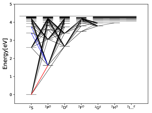
Our potassium model is complete up to $0.13$ eV below the first ionization energy ($4.34$ eV), with all available levels with configurations up to principal quantum number $n=20$ and the K II ground level. We have a total of $134$ levels in our atom, out of which $110$ are fine-structure-resolved energy levels from the NIST (2018) database, which comes primarily from Sugar & Corliss (1985) and Sansonetti (2008). The NIST (2018) database is complete up to orbital quantum number $l=3$, and the missing high-$l$ data were computed under the assumption that they are Rydberg levels ($24$ nonfine-structure-resolved levels).

The oscillator strengths of the allowed bound-bound radiative transitions were taken from Wiese et. al. (1969), Biemont & Grevesse (1973), and Sansonetti (2008). The total number of bound-bound transitions considered is 250. The Grotrian diagram of our atomic model can be seen in Figure 1. All bound-bound transitions involving the Rydberg levels are disregarded as it was seen that transitions with wavelengths larger than around $20000\ \AA$ had negligible impact on the statistical equilibrium. Therefore, these levels were added so that the code computes the partition function as accurately as possible. Whenever available, broadening data were added from the VALD database (Ryabchikova et al., 2015) or from Barklem et al. (1998).

3.2 Photoionization cross sections

The photoionization cross-sections of all levels between 4s and 7s are fine-structure resolved and were taken from Zatsarinny & Bartschat (2008) and Zatsarinny & Tayal (2010), calculated using the fully relativistic DBSR method. The photoionization cross-sections of the remaining levels were calculated using the hydrogenic approximation for bound-free transitions (Gray, 2005, Eq. 8.4). For higher levels, the cross sections of the two methods are more compatible with each other compared to the lower levels, and they start to diverge for increasingly higher wavelengths. Details and examples of the cross-sections can be seen in Figures 1-6 of Zatsarinny & Tayal (2010).

3.3 Collisional data

Figure 2: Ratio between e+K rate coefficients calculated through different methods. The triangles are the rates of the resonance transitions.

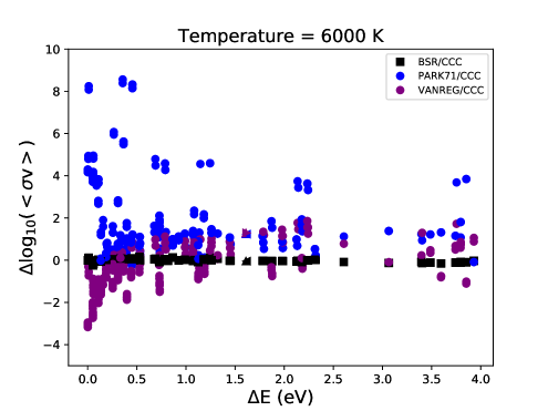
The inelastic e+K collisions have a large impact on the statistical equilibrium of potassium. As discussed in Sect. 2, the inelastic e+K collision rates for transitions between low-lying levels 4s and 6d were calculated using the CCC and BSR methods. Although CCC was employed in our standard atom, the e+K rates calculated via BSR were also tested, and the results with either method are indistinguishable; see Sect. 4.1. The rate coefficients for transitions from or to levels higher than 6d were all calculated using the Park71 method.

As mentioned in Sect. 2.3, in Figure 2 we compare the e+K rate coefficients calculated with the CCC, BSR, Park71, and vanReg62 methods at $6000$ K. We can see that CCC and BSR are in very good agreement, while the Park71 and vanReg62 methods differ from the two more recent and accurate methods. These disagreements lead to differences in the statistical equilibrium, and hence the synthetic lines, which are further explored in Sect. 4.1. We note that the rate coefficients of the resonance transitions 4p^3/2 - 4s^1/2 and 4p^1/2 - 4s^1/2 calculated via both the Park71 and the vanReg62 methods are very similar to each other (blue and purple triangles in Fig. 2).

The inelastic H+K collisions also influence the statistical equilibrium of potassium. For transitions involving low-lying levels (up to level 4f), we adopted the rate coefficients from Yakovleva et al. (2018), which are based on the LCAO model of Barklem (2016). Following Amarsi et al. (2018), we added these data to rate coefficients calculated using the free electron model in the scattering length approximation (Eq. 18, Kaulakys, 1991). The rate coefficients for transitions from or to levels higher than 6d were all calculated using the free electron model alone.

Finally, inelastic e+K collisional ionization was calculated using the empirical formula in chapter 3 of Allen (1976). These rates are important for guaranteeing LTE populations deep in the stellar atmosphere.

4 Non-LTE effects on Potassium

4.1 Test models

Table 2: Different atoms created to compare the collisions and photoionization recipes.

Atom designation

Electron excitation

Neutral hydrogen collisions

photoionization

	CCC	BSR	Park71	vanReg62	Barklem (2016)	Kaulakys (1991)	Zatsarinny & Tayal (2010)	Hydrogenic
a)Standard atom	X		X		X	X	X	X
b)BSR e+K		X	X		X	X	X	X
c)Park71 e+K			X		X	X	X	X
d)Hydrogenic photoionization	X		X		X	X		X
e)Resonance transitions only	X		X		X	X	X	X
f)No resonance transitions	X		X		X	X	X	X
g)Reduced H+K excitation	X		X		x$10^{-3}$	x$10^{-3}$	X	X
h)Reduced e+K excitation	x$10^{-3}$		x$10^{-3}$		X	X	X	X
i)vanReg62 e+K				X	X	X	X	X

Below we present the results of test calculations for the cases of different inelastic e+K collisional rates (CCC, BSR, Park71, and the vanReg62 calculations), and different photoionization calculations (the DBSR method by Zatsarinny & Tayal (2010) and the hydrogenic approximation). Our standard atom is atom a, discussed in Sect. 3. The collisions employed in each atom can be seen in Table 2. Atoms e and f have the same collisions as the standard atom but the first only has the resonance 4p^3/2 - 4s^1/2 and 4p^1/2 - 4s^1/2 radiative transitions and the second has all other transitions except those. Atom g has the H+K excitation rates decreased by a factor of $10^{-3}$; and atom h has the e+K excitation rates decreased by a factor of $10^{-3}$. The last atom (atom i) uses the vanReg62 e+K collisions.

4.2 Departure coefficients

Figure 3: Departure coefficients for the low-excited K I levels in the solar atmosphere.

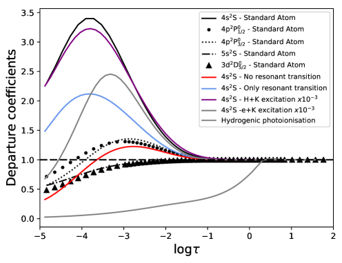
In Figure 3 we show a number of departure coefficients, b_k = n_NLTE /n_LTE, in the solar atmosphere, for our standard atom and for a number of our test atoms (Sect. 4.1), designed to test the main contributors to the non-LTE effects in potassium.

From Figure 3 and from previous works (e.g., Zhang et al., 2006), we see there is a strong overpopulation of the K I ground state and the two first excited states (4s, 4p^1/2 and 4p^3/2). The major drivers of this overpopulation are the resonance transitions due to photon losses. This was previously demonstrated in Sect. 4.3 of Bruls et al. (1992). According to their study, the infrared lines are also important in the statistical equilibrium (but to a much lower degree) and as such, Figure 3 illustrates that there are departures from LTE even when the resonance transitions are switched off (test atom f).

The departure coefficients also illustrate that the inelastic H+K excitation is of lesser importance on solar metallicity than the inelastic e+K excitation, in line with previous studies for alkali metals (Lind et al., 2009, 2011). This is further discussed in the following section through the analysis of synthetic lines.

4.3 Effects on spectral lines

Figure 4: Comparison between the synthetic spectral lines using different collisional recipes for the $5801\ \AA$ and $7698\ \AA$ lines in the 1D solar atmosphere (first and second panels). The third and fourth panels show the same but for a 1D metal-poor atmosphere (HD 84937) and a giant star 1D atmosphere, respectively.

To generate the synthetic spectral lines we employed MARCS (Gustafsson et al., 2008) 1D model atmospheres of the Sun with a potassium abundance of $A\rm{(K)}=5.11$, a metal-poor star with the same stellar parameters determined for HD 84937 in Peterson et al. (2017), and adopted by Spite et al. (2017), with a potassium abundance of $A\rm{(K)}=3.08$ ($T_{\mathrm{eff}}=6300$ K, log$g=4.00$ , [Fe/H]$=-2.25$ and $\xi=1.3\ \rm{km.s^{-1}}$), and a giant star with $T_{\mathrm{eff}}=4500$ K, log$g=1.5$, [Fe/H]$=-3.00$, $\xi=2.0\ \rm{km.s^{-1}}$, and [K/Fe]$=0.0$.

We first discuss how the different collisional and radiative data affect line formation in the solar atmosphere. The results for the $5801\ \AA$ and $7968\ \AA$ lines are shown in the first and second panels of Figure 4. We note that for all tests described in this section, the standard atom (a) and the atom replacing CCC collisions with BSR collisions (b) produce indistinguishable line profiles; as such we do not plot the results of the latter atom.

In our analysis, the high-excitation $5801\ \AA$ line is almost insensitive to departures from LTE. Consequently it is insensitive to the details of the non-LTE modeling, with variations of only around $0.01$ dex. Unfortunately, the line is very weak and can only be detected in very high-resolution and high-S/N spectra of stars with solar metallicity or higher, and solar effective temperature or cooler. Therefore, it is unsuitable for abundance analysis in representative samples. This $5801\ \AA$ line is however very sensitive to the large decrease in e+K excitation of atom h, a case in which the line is almost not formed and is much weaker than in LTE.

The resonance line has a different behavior. While the wings are insensitive to departures from LTE, the core is significantly deeper in non-LTE, as a result of the overpopulation of the ground state as we discussed in Sect. 4.2. There is a non-negligible difference between the line cores when using different collisional recipes.

Concerning the sensitivity of the non-LTE effects to the atomic data, the most prominent difference to the resonance line is observed when we decrease the e+K excitation rates by $10^{-3}$ (atom h). In this case the statistical equilibrium changes to the point where the line is not as deep as the LTE case, due to an increased importance of the photoionization – an effect also observed in the departure coefficient. The second largest difference is seen when the CCC collisions are replaced with the Park71 or vanReg62 collisions (atoms c and i): an abundance difference of $\Delta=+0.11$ dex with respect to the standard atom (a). The third largest difference is seen when adopting hydrogenic photoionization cross-sections (d): an abundance difference of $\Delta=+0.03$ dex with respect to the standard atom (a). When synthesizing the line with inefficient H+K collisions (g) the line core is deeper than the line from the standard atom (a), but the absolute abundance difference is the same as that produced by the atom with hydrogenic photoionization (atom d). The atom with only two radiative transitions, namely the resonance lines (e), has virtually the same abundance as our standard atom.

The non-LTE effects are mainly a source-function effect caused by photon losses (resonance scattering). Like in the Na D lines (see Sect 3.1 of Lind et al., 2011), the overpopulation of the ground state pushes the mean formation depth outward, deepening the lines – but only slightly. The main effect that deepens the spectral line is the sub-thermal line source function. The line source function of a line formed by pure resonance scattering is determined by the radiation field, and therefore by the radiative rates in the lines themselves. This is why the atom with only the resonance lines (e) performs so similarly to the standard atom (a), that is, because the source function is the same in the two cases.

In the third panel of Figure 4 we show the synthetic spectral lines in a metal-poor turn-off star. Similarly to the solar atmosphere case, for HD 84937, compared to the standard atom (a), the non-LTE effects change the most when the e+K collisions are reduced (h), whereas reducing the H+K collisions (g) has only a small impact. The largest abundance differences ($\Delta=+0.04$ dex) are for atoms c, e, and i. The third largest is for atom d ($\Delta=+0.01$ dex). The general difference between the synthetic lines in HD 84937 is smaller than in the solar atmosphere, because in a metal-poor atmosphere the hydrogen collisions are more relevant to the statistical equilibrium, owing to the reduced number of free electrons.

The stars analyzed in this work are late-type stars, in which the H+K excitation is expected to be less important than in giant stars. In the last panel of Figure 4 we tested the differences in a giant star. In this case the lines using the standard and the c atoms are indistinguishable. This happens because in this metal-poor giant star there are not as many free electrons and the contribution of this process becomes less important. Although less important, the effect of the vanReg62 e+K collision rates, which are mostly higher than the other methods employed, can be observed as it increases the depth of the line core. Nevertheless, as the importance of the e+K collisions decreases, we observe that the importance of the H+K excitation increases: compared to the standard atom (a), there is an abundance difference of $\delta\approx 0.03\,\mathrm{dex}$ after reducing the efficiency of the H+K collisions (g). This can be contrasted with the late-type metal-poor star HD 84937 (third panel of Figure 4), where no appreciable difference is observed.

In this section, we showed that the use of improved calculations of electron collisions is the most influential factor in the non-LTE line profile of dwarfs. The CCC and BSR calculations give comparable results, but substituting these calculations with the older Park71 and vanReg62 methods considerably changes the strength of the synthetic lines. Improved photoionization cross-section calculations with the DBSR method also had non-negligible differences in the final line depth of the synthetic lines, and are important for accurate abundance determinations through the $7698\ \AA$ resonance line.

5 Abundance analysis of K in benchmark stars

Table 3: Stellar parameters of the sample.

Star	Teff (K)	$\log\ g$ ($g$ in $\rm{cm.s^{-2}}$)	$\xi$ ($\mathrm{km\,s^{-1}}$)	[Fe/H]	Broadening* ($\mathrm{km\,s^{-1}}$)
Sun	$5772^{a}$	$4.44^{a}$	$1.0^{b}$	$0.00^{c}$	$3.5$
HD 192263	$4998^{d}$	$4.61^{d}$	$0.66^{e}$	$-0.05^{e}$	$3.0$
Procyon	$6556^{f}$	$4.01^{f}$	$1.85^{g}$	$-0.02^{h}$	$6.0$
HD 103095	$5140^{i}$	$4.69^{j}$	$0.9^{k}$	$-1.13^{l}$	$1.0$
HD 140283	$5787^{i}$	$3.66^{m}$	$1.6^{g}$	$-2.28^{n}$	$3.8$
HD 84937	$6371^{d}$	$4.05^{o}$	$1.3^{p}$	$-1.97^{n}$	$5.0$

Table 4: Atomic data of the transitions

$\lambda\ (\AA)$	Transition	E (eV)	log($gf$)	$\sigma/a^{2}_{0}$	$\alpha$
$5801.75$	4p2P${}^{0}_{3/2}$ - 7s2S1/2	$1.617-3.753$	$-1.605$	–	–
$6938.77$	4p2P${}^{0}_{3/2}$ - 6s2S1/2	$1.617-3.403$	$-1.252$	$1721$	$0.294$
$7698.96$	4s2S1/2 - 4p2P${}^{0}_{1/2}$	$0.000-1.610$	$-0.176$	$485$	$0.232$
$12522.16$	4p2P${}^{0}_{3/2}$ - 5s2S1/2	$1.617-2.607$	$-0.134$	$1260$	$0.183$

We further tested our standard atom by modeling the K I optical lines in different stellar atmospheres. We analyzed the Sun and the following benchmark stars of the GAIA-ESO spectroscopic survey: HD 84937, HD 103095, HD 192263, HD 140283 and Procyon. For the Sun we use the Stenflo (2015) flux solar atlas, and the spectra of the remaining objects are high-resolution (R$\approx 220000$) PEPSI spectra (Strassmeier, Ilyin & Weber, 2018); these are available fully reduced and continuum normalized . The stellar parameters of the stellar model atmospheres can be seen in Table 3.

To determine the potassium abundances of the stars we match synthetic equivalent widths (EWs) to observed ones. We tested both Gaussian fitting and full line integration for measuring the EWs in the observed spectra and the methods have similar outcomes. We convolved (Gaussian Kernel) the synthetic spectra of the best abundance to account for rotational and macroturbulence velocities using the PyAstronomy python package. Both are treated as a free parameter but for a first guess we calculate the macoturbulent velocity using the trend with $T_{\mathrm{eff}}$ described in Gray (2005).

We analyzed three observable lines in the optical spectral region: the K I $5801.7$, $6938.7,$ and $7698.9\ \AA$ lines, and for completeness added the $12522\ \AA$ infrared line in the Sun. The atomic data of the transitions are in Table 4. We used standard MARCS (Gustafsson et al., 2008) model atmospheres. In contrast with Zhang et al. (2006) and Scott et al. (2015) we did not analyze the K I $4044.1$ and $7664\ \AA$ lines because they are heavily blended. We show the fitted lines in Figures 5 to 9.

We estimate a lower bound on the modeling errors through the line-to-line scatter of the three observable lines in the Sun and HD 192263. In the Sun, the scatter is only $0.02$ dex, but it is up to $0.05$ dex in HD 192263, possibly due to the strong damping wings and difficulties in determining the abundance through the resonance line in this star (both are further discussed below). Most of our analyzed stars do not show such strong damping wings and asymmetries observed in HD 192263, and therefore the uncertainties are not as high. Thus, we estimate a lower error of $0.03$ dex for our measurements.

5.1 Sun

Figure 5: Non-LTE abundance fit of the $5801$, $6939$, $7698$, and $12522\ \AA$ lines (top left, top right, lower left, and lower right, respectively) at the Sun with an abundance of $A\rm{(K)}=5.11$. The LTE lines of the same abundance are also shown in the plots.

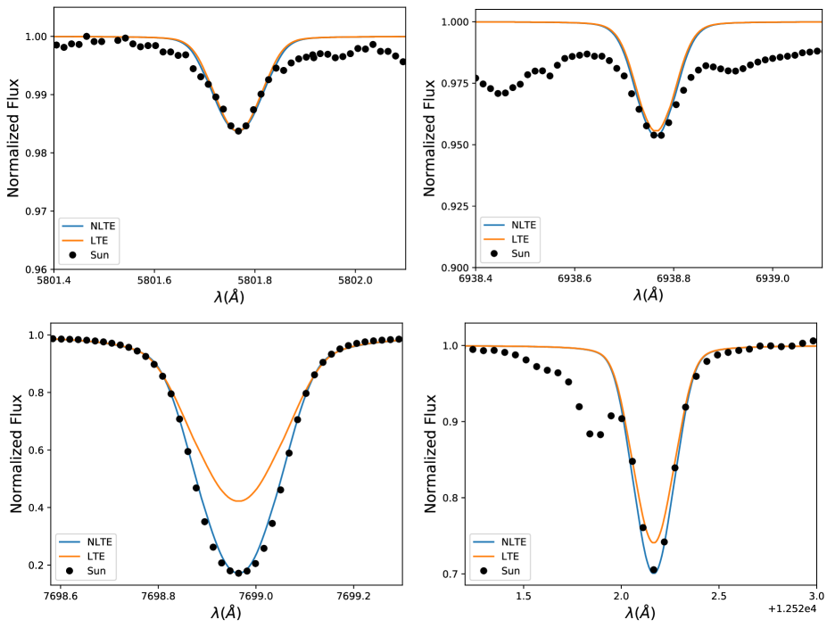
For the Sun we derived a 1D non-LTE abundance of $A\rm{(K)}=5.11$ from averaging the result of the best EW match of the three optical lines in the solar spectrum. In our analysis the individual abundances of each line found were $A\rm{(K)}_{\rm{5801\ \AA}}=5.10$ dex, $A\rm{(K)}_{\rm{6939\ \AA}}=5.10$ dex, and $A\rm{(K)}_{\rm{7698\ \AA}}=5.12$. Zhang et al. (2006) did not find, for these same lines, abundances in such good agreement. Their abundances vary up to $0.09$ dex between the optical ($A\rm{(K)}_{\rm{5801\ \AA}}=5.15$, $A\rm{(K)}_{\rm{6939\ \AA}}=5.06,$ and $A\rm{(K)}_{\rm{7698\ \AA}}=5.14$). With 1D MARCS model atmospheres (such as those used here) Scott et al. (2015) analyzed the lines $5801\ \AA$ and $6939\ \AA$, finding $A\rm{(K)}_{\rm{5801\ \AA}}=5.15$ with a non-LTE correction of $-0.03$ dex, in good agreement with our abundance. For the other line in common they determined $A\rm{(K)}_{\rm{6939\ \AA}}=5.09$, and applied a correction of $-0.03$ dex, a somewhat smaller abundance than what we found ($0.04$ dex) but still within their expected error of $0.05$ dex for potassium.

For our plot we needed to apply a change in the original normalization of the $5801$ and $6939\ \AA$ lines. As already pointed out by Zhang et al. (2006) there are terrestrial blends around the $5801\ \AA$ line and a very uncertain continuum at the $6939\ \AA$ region due to a number of contributions from different lines. We optimized the continuum of those lines based on adjacent regions ($5811\ \AA$ and $6935\ \AA$).

It must be noted that adjacent features were not synthesized, and the potassium lines at $5801$, $6939$, and $12522\ \AA$ were synthesized with the best abundance and a broadening parameter determined via the fitting of the $7698\ \AA$ line. As mentioned above, the abundances were not calculated via synthetic spectra. We separately measured the EW of each observed line and matched them to the EWs of the synthetic lines to find the abundances. Thus, the fits shown in Figure 5 were not used to estimate the abundances, and the line profiles are shown only to demonstrate that our EW abundance can reproduce the lines. As can be seen, the synthetic line fits to the solar spectra are very good. We also show the LTE line of the same abundance as a comparison and one can see that although the differences between the LTE and non-LTE methods for the $5801\ \AA$ and $6939\ \AA$ lines are very small (to fit the lines with LTE one needs an abundance $\approx 0.01$ dex higher than the non-LTE abundance), the difference observed for the resonance $7698\ \AA$ line is very large. In the case of the resonance line, the LTE assumption fails completely and it is not possible to correctly reproduce the spectral line, even when considerably increasing the abundance of K I to $A\rm{(K)}\approx 5.44$ (our best LTE abundance via EW). We emphasize the importance of taking non-LTE effects into account when studying the GCE of potassium using the resonance line (e.g., Takeda et al., 2002; Zhang et al., 2006; Takeda et al., 2009; Andrievsky et al., 2010; Scott et al., 2015).

5.2 HD 84937

Figure 6: Non-LTE abundance fit of the $7698\ \AA$ line for HD 84937 with an abundance of $A\rm{(K)}=3.15$. The LTE line of the same abundance is also shown in the plot.

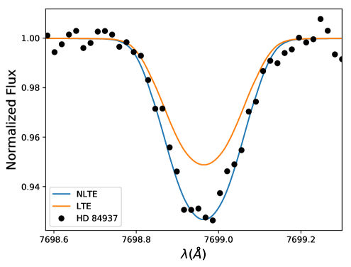
HD 84937 is a low-metallicity ([Fe/H]$=-1.97$), bright, main sequence turn-off star that is commonly used as a standard representative of the abundance pattern of similar-metallicity field stars.

Spite et al. (2017) analyzed the abundance pattern of this star and measured a LTE potassium abundance of $A\rm{(K)}=3.40$ from the resonance $7698\ \AA$ line. These latter authors applied a non-LTE abundance correction of $-0.2$ dex from Zhang et al. (2006), finally advocating $A\rm{(K)}=3.20$ for this line in HD 84937.

In non-LTE, we measured $A\rm{(K)}=3.15$, while our best LTE abundance is $A\rm{(K)}=3.33$, a difference of $\Delta=-0.18$ dex, in excellent agreement with the correction from the model atom described in Zhang et al. (2006) and used in Spite et al. (2017). In Figure 6 we show the non-LTE abundance along with the LTE synthetic line of the same abundance for comparison. As can be seen, the non-LTE abundance that was found fits the stellar spectrum very well. The small asymmetry in the red wing of the observed spectral line is due to convective motions in the stellar atmosphere, the same conclusion as drawn from the analysis of this line by Smith et al. (2001). The best LTE line was also able to reproduce the observed line and the best non-LTE is indistinguishable from the best LTE line when plotted together.

5.3 HD 103095

Figure 7: Non-LTE abundance fit of the $7698\ \AA$ line for HD 103095 with an abundance of $A\rm{(K)}=4.00$. The LTE line of the same abundance is also shown in the plot.

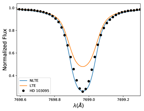
HD 103095 is a metal-poor K-type dwarf, commonly used as a standard star of the inner Halo. This star is an $\alpha$-poor star with [Mg/Fe]$=0.12$ dex (Reggiani & Meléndez, 2018), which is lower than usually found for stars of such metallicity.

When assuming LTE, we determined an abundance $A\rm{(K)}=4.26$ for this star. When the non-LTE modeling was used instead, the best match of EW was found for an abundance of $A\rm{(K)}=4.00$, a difference of $-0.26$ dex. The non-LTE synthetic line, the observed spectra, and the comparison LTE synthetic line can be seen in Fig. 7. The spectral line in HD 103095 is very well reproduced under non-LTE, except for a small discrepancy in the near-to-core region, which might be caused by 3D effects (further discussed in Sect. 6). As for LTE, our best abundance estimate was not able to correctly reproduce the line.

5.4 HD 140283

Figure 8: Non-LTE abundance fit of the $7698\ \AA$ line for HD 140283 with an abundance of $A\rm{(K)}=2.77$. The LTE line of the same abundance is also shown in the plot.

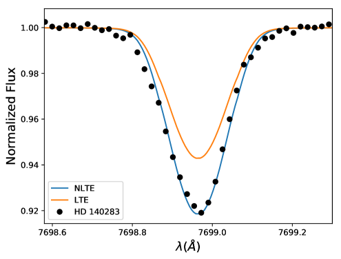
HD 140283 is a bright very metal-poor, high-velocity subgiant in the solar neighborhood. Its proximity to the Sun made it the first star with spectroscopic confirmation of chemical abundances lower than what is found in the Sun (Chamberlain & Aller, 1951; Sandage, 2000). Its brightness and proximity to the Sun means it has a well-determined parallax and also a well-determined age. Furthermore, it is one of the oldest stars with very reliable age estimation (Bond et al., 2013).

The best LTE abundance we found for HD 140283 was $A\rm{(K)}=2.95$ and the final non-LTE abundance is a very low abundance of $A\rm{(K)}=2.77$ (or [K/Fe]$=-0.06$ dex), which is lower than the mean non-LTE abundance we found for stars in the metallicity regime $-2.2\leq$[Fe/H]$\leq-2.5$ of [K/Fe]$=+0.21$ dex; see Fig. 14. This lower-than-usual abundance was not expected, but the LTE abundance we found matches the LTE abundance given by the radiative-transfer code MOOG (Sneden, 1973) using the same stellar information.

Although the best abundance is not as high as we expected for the metallicity of the star, the abundance we found fits very well to the observed spectra and the resulting profile appears to be very reliable. Like in HD 84937, if the best LTE abundance is plotted on top of the best non-LTE abundance the two lines are almost indistinguishable, with the non-LTE line being very slightly deeper. In Figure 8 we show the non-LTE and LTE line of K with an abundance of $A\rm{(K)}=2.77$.

5.5 HD 192263

Figure 9: Non-LTE abundance fit of the $5801$, $6939,$ and $7698\ \AA$ lines (top, middle, and lower panels, respectively) for HD 192263 with an abundance of $A\rm{(K)}=5.03$. The LTE lines of the same abundance are also shown in the plots.

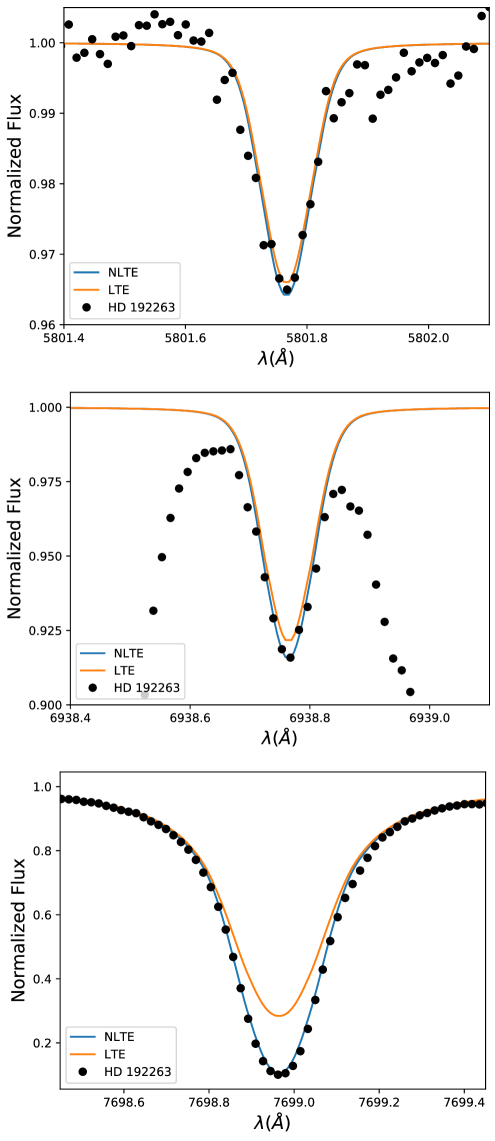
HD 192263 is a cool dwarf star of nearly solar metallicity, and is also a Gaia-ESO benchmark star. Under its atmospheric conditions, the $7698\ \AA$ line develops strong damping wings and it is possible to visually perceive the asymmetries at the wings of the line, as shown in Figure 9. It is difficult to reproduce the potassium line even under non-LTE.

In this star, it is possible to detect not only the resonance line, but also the other two clean potassium spectral lines. We therefore determined the abundance of this star by measuring the EW of the three lines ($5801\ \AA$, $6939\ \AA$, and $7698\ \AA$) and found the non-LTE abundances of $A\rm{(K)}=5.07$, $5.02,$ and $5.01,$ respectively. The adopted value is the averaged value of $A\rm{(K)}=5.03$.

The LTE abundances of the $5801\ \AA$ and $6939\ \AA$ lines were found to be $A\rm{(K)}=5.04$, which is consistent with the non-LTE abundances. The $7698\ \AA$ LTE abundance is $5.26$, a non-LTE correction of $-0.23$ dex.

We show the spectra and the synthetic lines of the $5801$, $6939,$ and $7698\ \AA$ lines in Figure 9. The observed spectra can be reproduced by the non-LTE synthetic spectra but in HD 192263 the synthetic line of the best LTE abundance found could not reproduce either the core or the wings of the observed line. Both in LTE and non-LTE there is an asymmetry at the red wing that has the same form as the asymmetry observed in Procyon (Sect. 5.6 and further discussed in Sect. 6).

5.6 Procyon

Figure 10: Non-LTE abundance fit of the $7698\ \AA$ line for Procyon with an abundance of $A\rm{(K)}=4.86$. The LTE line of the same abundance is also shown in the plot.

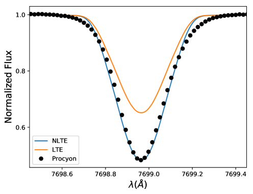
Procyon is a solar metallicity F-type star very close to the Sun, in which the only observable K line is the resonance line $7698\ \AA$. The wings of the line are very broad and difficult to correctly model. The non-LTE abundance, based on the EW of the line, fails to reproduce the wings; the red wing is more broadened than the blue wing, as also observed in HD 192263, an effect that is known to be a result of granulation in the stellar atmosphere (e.g., Dravins et al., 1981). Takeda et al. (1996) were able to model the wings of Procyon, but they applied corrections by hand to the red wing of the line and to the line core in order to correct what they believed to be unfavorable instrumental effects in their measurements.

As can be seen in Figure 10 the line core is well represented by the non-LTE synthetic line, while the broadened wings of the observational spectra diverge near the continuum level. We found a non-LTE abundance of $A\rm{(K)}=4.86$ and a LTE abundance of $A\rm{(K)}=5.54$, a correction of $-0.68$ dex. Takeda et al. (1996) analyzed the potassium abundance in Procyon and also found a non-LTE correction of $\approx-0.7$ dex, although their LTE and non-LTE abundances are higher than what we found. We note again that even in non-LTE a 1D model could not simultaneously reproduce the core and the wings of the potassium $7698\ \AA$ line in Procyon. As before, we also show the LTE line of the same abundance ($A\rm{(K)}=4.86$) in Fig. 10.

6 Three-dimensional non-LTE

Figure 11: Synthetic non-LTE $7698\ \AA$ potassium line under different atmospheric model assumptions (1D and 3D).

In Sect. 5 we demonstrated that there are severe (1D) non-LTE effects on the potassium resonance line, and that non-LTE methods are therefore needed to obtain reliable estimates of potassium abundances. This was particularly observed through the abundances of the Sun and HD 192263, in which one can measure all three optical lines, including those not heavily affected by non-LTE effects. In those cases only a non-LTE analysis can simultaneously give us consistent abundances in all observable lines.

However, although we can correctly reproduce the core of the $7698\ \AA$ line, the wings are not as well reproduced, an effect that is observable in the spectra of HD 192263 (Sect. 5.3) and Procyon (Sect. 5.6). In Procyon one can clearly see the existence of an asymmetry between the blue and red wings of the line.

These types of asymmetries are associated with convection effects and can only be correctly modeled by using a 3D radiation-hydrodynamical simulation of the stellar atmosphere (Dravins et al., 1981; Asplund et al., 2000, 2004). A great amount of effort has been invested in the modeling of the convection-induced asymmetry of the lithium resonance line, which is similar to potassium in many respects. In particular, many have attempted to disentangle the imprint of convection with possible absorption in the red wing due to ⁶Li (e.g., Smith et al., 2001; Asplund et al., 2006). The importance of accounting for non-LTE effects combined with the 3D line formation of lithium has also been emphasized (Cayrel et al., 2004; Lind et al., 2013).

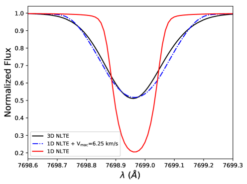
The asymmetric shape of the potassium resonance line has been studied in the context of solar granulation for decades (e.g., Marmolino et al., 1987). However, although there have been studies modeling the resonance line formation using 3D LTE models (e.g., Nissen et al., 2000; Scott et al., 2015) there is, to the best of our knowledge, no published 3D non-LTE study of potassium. Although a full quantitative analysis is outside the scope of this project, we explored the effects with the radiative-transfer code BALDER (Amarsi et al., 2018). We ran one snapshot of a full 3D non-LTE calculation based on a STAGGER (Magic et al., 2013) model atmosphere with $T_{\mathrm{eff}}=6437$ K, log $g=4.0$, [Fe/H]$=0.0,$ and [K/Fe]$=0.0$, which correspond to similar parameters to those of Procyon.

Our results showed that 1D non-LTE can only partially reproduce the wings seen in 3D after we added strong macroturbulent broadening effect of V_MAC $\approx 6.25$ km/s (dashed line), and even so the 1D non-LTE does not fully reproduce the wings seen in 3D, particularly the asymmetry of the line.

The 3D non-LTE feature that we synthesized indicates that the misrepresentation of the wings in our 1D non-LTE analysis is due to unaccounted-for 3D effects. Although the asymmetries of the potassium resonance wings are much better represented in full 3D non-LTE we argue that the EW analysis of the 1D non-LTE yields comparable results.

7 Non-LTE corrections grid

Figure 12: Contour diagram illustrating the abundance corrections in [Fe/H]$=0.0$ (upper panel) and [Fe/H]$=-3.0$ (lower panel) for the $7698\ \AA$ line.

Figure 13: The top panel shows how the non-LTE corrections vary with EW. The lower panel shows the non-LTE correction variation with [Fe/H]. In both panels we have two different model atmospheres and both show the corrections for the $7698\ \AA$ line.

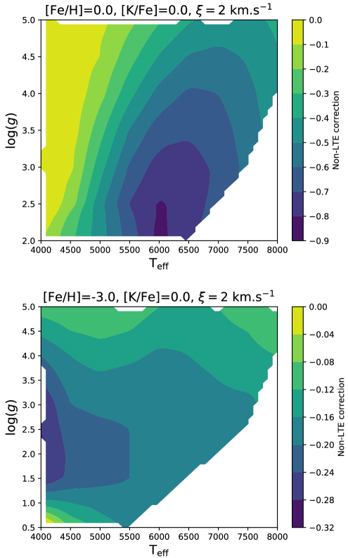
Using our standard atom we produced a grid of non-LTE corrections, for model atmospheres of different stellar parameters. Our grid was computed for models with effective temperatures in the range $4000\leq\rm{T}_{\rm{eff}}\ /\rm{K}\leq 8000$ with steps of $500$ K; for each T_eff the surface gravity range is $0.5\leq\rm{log}(g)\leq 5.0$ dex in steps of $0.5$, and we also vary the metallicities in the range $-5.00\leq$ [Fe/H] $+0.50$ in steps of $0.25$ and use microturbulence velocities of $\xi=1.0$, $2.0,$ and $5.0$ $\rm{km/s}$. We determined synthetic spectral lines of potassium abundances varying in the range $-1.25\leq$[K/Fe] $\leq+1.25$, and estimated the LTE and non-LTE EWs in each case. Thus, we obtained a final grid with synthetic LTE and non-LTE EWs for each calculated abundance in each model atmosphere.

In Figure 12 we show an example of the non-LTE corrections for solar metallicity varying the stellar parameters. The abundance correction for a Sun-like star is approximately $-0.3$ dex and for stars like Procyon the abundance correction is as high as $-0.7$ dex.

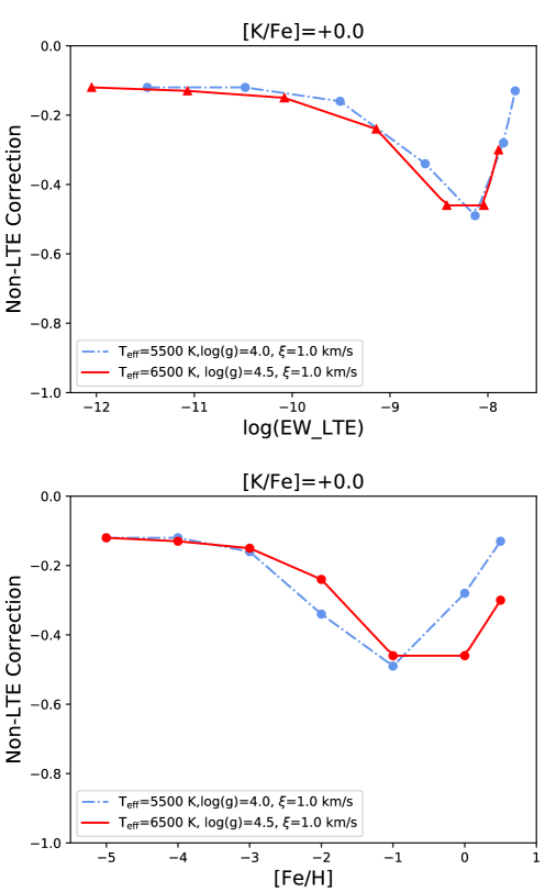
From the top panel of Figure 13 we can see that the correction is very dependent on line strength, and the apparent dependence with temperature seen in Fig. 12 is an indirect effect. The extremely high non-LTE corrections for certain stellar atmospheres shows us that it is imperative to apply non-LTE corrections when analyzing the abundances of potassium from the resonance lines.

In the lower panel of Figure 13 we show the dependence with metallicity of two model atmospheres for a K abundance of [K/Fe]=0.0. An important dependence with metallicity starts to appear at [Fe/H] greater than $-2.0$; this can be directly related to the line becoming stronger for higher metallicities and saturating. As the metallicity increases and the line gets stronger, the corrections are larger and peak at approximately solar metallicity before decreasing again. However, we have not found any measurements of potassium in stars with metallicities higher than solar, and therefore this decrease in the corrections after [Fe/H]=0.0 has not been applied in any observational data to test its compatibility with the GCE models.

We also computed the corrections for the resonance $7664\ \AA$ line and the infrared lines $15163\ \AA$ and $15168\ \AA$ (which are in the APOGEE range). Abundances from the resonance $7664\ \AA$ line must also be non-LTE corrected as the corrections are on the same order as the corrections computed for the $7698\ \AA$ line, but the infrared lines do not have such strong non-LTE dependence (the mean correction of the $15168\ \AA$ for [K/Fe]$=0.0$ at the same models presented in Figure 13 are $-0.03$ and $-0.06$ dex).

Our final grid is publicly available as an electronic table.

8 Chemical evolution of Potassium

8.1 Metal-poor stars

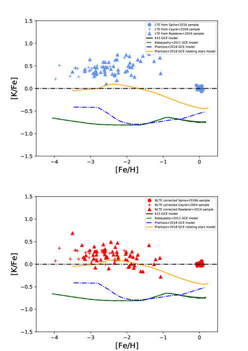
We applied our grid of corrections to a series of abundances from several publications in order to study the evolution of potassium in our galaxy. We show these results and compare them to the K11 (Kobayashi et al., 2011), K15 (Zhao et al., 2016; Sneden et al., 2016) GCE models, and the models from Prantzos et al. (2018) with and without yields from massive rotating stars.

We determined abundances under LTE using the 1D LTE code MOOG (Sneden, 1973) based on three sets of published EWs: Cayrel et al. (2004), Roederer et al. (2014), and Spina et al. (2016). We then determined the non-LTE abundances by applying non-LTE abundance corrections from our grid. Andrievsky et al. (2010) recently reanalyzed the Cayrel et al. (2004) sample with their non-LTE corrections and we compared our results to theirs, finding a mean difference of $\sim-0.1$ dex in the final non-LTE abundances (with their abundances being higher).

Figure 14 and Table LABEL:nlte_cor_abnd_table show both the [K/Fe]_LTE and the [K/Fe]_NLTE results for the above-mentioned samples. In the upper panel of Fig. 14 we see the behavior of the LTE abundances. For all data there is a large discrepancy between the abundances of models and observations, reaching up to $1$ dex. For [Fe/H]$\lesssim-1.0$, the LTE potassium abundances show an increasing trend with [Fe/H], which is similar to what is predicted by the Kobayashi et al. (2011) model, but differs from the behavior of the Prantzos et al. (2018) models.

The non-LTE abundances however show a different result. In the region [Fe/H]$\lesssim-1.0$, there is no longer a trend of increasing potassium abundances with increasing [Fe/H]; rather, the potassium abundances gradually decrease. The model of rotating massive stars by Prantzos et al. (2018) appears to correctly reproduce the observations, although the mean observed abundance is slightly higher than the model. Non-LTE corrected abundances and the model of massive rotating stars show the same behavior: a small increase in abundances between $-3\leq$ [Fe/H] $\leq-2$ followed by a decrease in abundances with increasing metallicity. On the other hand, the models from Kobayashi et al. (2011) and the Prantzos et al. (2018) model without rotation underestimate the production of potassium and their yields clearly fail to reproduce the observations.

8.2 Solar twins

The solar twin sample of Spina et al. (2016) sits at [Fe/H]$\approx 0.0$ in Fig. 14. Correcting the abundances for non-LTE effects does not have a significant effect here. This is because these abundances were measured in a line-by-line differential analysis with respect to the Sun. To first order, the non-LTE errors in the analysis of the solar twin spectra cancel with the non-LTE errors in the analysis of the solar spectrum. However, the non-LTE corrections lead to a reduction in the scatter of the potassium abundances, as we discuss below.

Figure 14: (Top panel) LTE abundances calculated using MOOG and the EWs from Cayrel et al. (2004), Roederer et al. (2014), and Spina et al. (2016). (Lower panel) Non-LTE corrected abundances (from the LTE abundances in the upper panel). The LTE and non-LTE corrected abundances (in A(K)), are shown in Table LABEL:nlte_cor_abnd_table. In both panels we also show three different GCE models: in black the model from Kobayashi et al. (2011); in dashed blue and orange the models from Prantzos et al. (2018) without and with yields from massive rotating stars, respectively.

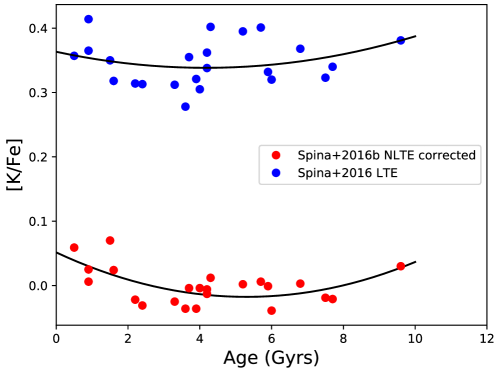
In their high-precision differential analysis of solar twins (stars with atmospheric parameters similar to the solar parameters - $\Delta\rm{T}_{\rm{eff}}\pm 100$ K, $\Delta\rm{log}(g)\pm 0.1$ dex, $\Delta\rm{[Fe/H]}\pm 0.1$ dex and mass within $\approx 5\%$ of the solar mass) Spina et al. (2016) analyzed 20 elements and for all of them, except potassium, they found a tight relationship between stellar age and [X/Fe], with strongly varying slope depending on the element. With this in mind we reanalyzed their sample of solar twins and the same plot of [K/Fe] versus age can be seen in Fig. 15. The trends with stellar age of the LTE and the non-LTE abundances are the same. Being solar twins, not only are the abundances very similar to one another, but also the non-LTE corrections. Although this result was expected, we call attention to the fact that the non-LTE abundances have a smaller scatter than the LTE abundances. This means that the non-LTE abundances might be more reliable, as the abundances of solar twins are very homogeneous and similar to the solar abundance (Bedell et al., 2018). This is also important because it shows that even in a differential abundance analysis of solar twins, non-LTE corrections play an important role in explaining the evolution of the elements by decreasing the scatter of abundance measurements, which might further improve fits of their behavior. The reduced scatter is important to correctly assess the homogeneity of chemical evolution and therefore to draw more precise conclusions on the nucleosynthetic mechanisms that drive potassium evolution throughout cosmic history. The reduced scatter is also important to assess the homogeneity of different stellar populations (e.g., thin/thick disk) and stellar associations (clusters or binaries), which is also relevant for chemical tagging, a popular application of stellar spectroscopy.

As already mentioned, Spina et al. (2016) found a function able to describe [X/Fe] abundances over cosmic time for all elements analyzed, apart from potassium. We also tried to find a function to describe [K/Fe] over time with our lower scatter non-LTE abundances, but as in Spina et al. (2016) we did not find a function that can describe its behavior. Figure 15 shows a fourth-degree polynomial function that was used only to demonstrate the smaller scatter of the non-LTE data. The standard deviations of the non-LTE-corrected and the LTE abundances are $0.027$ dex and $0.035$ dex, respectively, an improvement of $\sim 23\%$. Within $1\sigma$ the LTE and non-LTE fits are the same.

It is interesting how there is no possible fit to the potassium abundances over time, as found for the other elements. This might indicate an inhomogeneous enrichment of potassium, although the small scatter we observe might be caused by errors in the analysis. If indeed the ISM was not fully homogenized with K, the small abundance differences among stars born in different sites in the Galaxy could explain this uncanny inability to fit the abundances. This behavior could be explained by a GCE where rotating massive stars play a role. As the occurrence of such objects is not as common as, for example, type II supernovae, rotating massive stars might be able to produce these localized small inhomogeneities, which would depend on a localized mass function and the production of the rotating massive stars. This localized effect would not be seen in most of the other commonly measured elements (such as C, O, Na, Mg, Al, Si, etc) because, as one can see in Fig. 13 of Prantzos et al. (2018), most of them have an evolution that is not significantly influenced by massive rotating stars, as both models (with and without the massive rotating stars) have virtually the same results. However, we caution that such small scatter might also be caused by errors in our analysis, and that the inability to fit the solar-twin data might simply be because the empirical fits suggested are not adequate.

Figure 15: In red we show the non-LTE abundances of the Spina et al. (2016) sample and in light blue the scaled LTE abundances. The offset is due to the use of the same solar potassium abundance LTE and non-LTE.

9 Conclusions

We built a new model atom of potassium in order to test the non-LTE effects in stellar abundances estimations. We used state-of-the-art calculations of neutral hydrogen and electronic collisional cross-sections and photoionization cross-sections.

The use of improved calculations of electron collisions were the most influential factor in the non-LTE line profile of the late-type stars and both CCC and BSR calculations give comparable results. The choice between the different H+K collisions and the DBSR photoionization cross-sections also had non-negligible and similar effects on the final line depth of the synthetic lines, and their contribution is more relevant to the analysis of giant stars. The use of different collisional recipes can lead to differences of up to $0.1$ dex in the abundance analysis. With the aid of an atom with only the resonance transitions we concluded that the major driver of the non-LTE effects is the photon losses in the $7664$ and $7698\ \AA$ lines.

As test cases for the quality of our synthetic spectra, we derived the potassium abundance of the Sun and other benchmark stars. We found that our non-LTE synthetic spectra are a good fit to the stellar spectra, as opposed to what is seen in LTE. When available the abundances were derived from the three optical spectral lines and the results are very homogeneous with the non-LTE approach, and vary considerably if every line is analyzed in LTE. Through this analysis we also showed that there are important 3D effects that can be observed via the asymmetries in the wings of the potassium line. The differences of the 1D and 3D line profiles were shown for a test case and we see that EW analyses of 1D non-LTE and 3D non-LTE lines give similar results, which is valuable to validate the grid of corrections that was developed for this work.

Finally, we used our grid of corrections on three sets of potassium data to analyze the chemical evolution of the Galaxy. We see that the yields of the common models (Figure 14) are not enough to explain the observational data. However, the model with yields from rotating massive stars by Prantzos et al. (2018) is able to partially reproduce the core of the observed abundances, especially the decrease in abundance for metallicities higher than [Fe/H] of around $-2.5$ dex, which we also observe in our non-LTE results from the Roederer et al. (2014) sample. All the GCE models fail to reproduce the observed abundances at solar metallicity. However, the decreased scatter in the solar twins is an important result as it shows that the LTE differential abundance is not fully free of systematic uncertainties due to line formation responsible for part of the observed inhomogeneities, and will help constrain the nucleosynthetic mechanism mainly responsible for potassium production in this narrow metallicity range.

Appendix A Non-LTE corrected abundances

1]

Table 5: Non-LTE corrected abundances. Stellar parameters and LTE abundances are from Spina et al. (2016); Cayrel et al. (2004) and Roederer et al. (2014)

Star	Teff (K)	$\log\ g$ ($g$ in $\rm{cm.s^{-2}}$)	[Fe/H]	$\xi$ ($\rm{km.s^{-1}}$)	KNLTE	KLTE
18Sco	$5818$	$4.46$	$0.05$	$1.00$	$5.14$	$5.48$
HIP 56948	$5793$	$4.47$	$0.02$	$1.00$	$5.10$	$5.44$
HIP 102152	$5724$	$4.36$	$-0.01$	$1.00$	$5.08$	$5.44$
HD 20630	$5744$	$4.49$	$0.06$	$1.10$	$5.23$	$5.53$
HD 202628	$5831$	$4.51$	$0.00$	$1.00$	$5.13$	$5.47$
HIP 30502	$5736$	$4.42$	$-0.06$	$1.00$	$5.01$	$5.37$
HIP 73815	$5800$	$4.33$	$0.03$	$1.10$	$5.14$	$5.50$
HIP 77883	$5701$	$4.37$	$0.02$	$1.00$	$5.11$	$5.45$
HIP 89650	$5853$	$4.42$	$-0.01$	$1.10$	$5.09$	$5.46$
HD 9986	$5827$	$4.44$	$0.09$	$1.00$	$5.17$	$5.51$
HD 13531	$5653$	$4.53$	$0.02$	$1.20$	$5.15$	$5.45$
HD 13931	$5895$	$4.29$	$0.07$	$1.10$	$5.19$	$5.58$
HD 32963	$5768$	$4.37$	$0.09$	$1.00$	$5.20$	$5.53$
HD 33636	$5963$	$4.47$	$-0.08$	$1.10$	$5.04$	$5.44$
HD 43162	$5661$	$4.53$	$0.06$	$1.20$	$5.24$	$5.52$
HD 45184	$5873$	$4.41$	$0.07$	$1.00$	$5.18$	$5.54$
HD 87359	$5700$	$4.47$	$0.07$	$0.90$	$5.18$	$5.48$
HD 95128	$5904$	$4.35$	$0.02$	$1.10$	$5.13$	$5.53$
HD 98618	$5845$	$4.42$	$0.05$	$1.10$	$5.12$	$5.48$
HD 106252	$5885$	$4.42$	$-0.07$	$1.10$	$5.05$	$5.44$
HD 140538	$5704$	$4.48$	$0.06$	$0.90$	$5.13$	$5.45$
HD 143436	$5825$	$4.43$	$0.04$	$1.00$	$5.14$	$5.49$
HD 112257	$5686$	$4.30$	$-0.00$	$0.90$	$5.14$	$5.49$
HD 2796	$4950$	$1.50$	$-2.47$	$2.10$	$2.88$	$3.13$
HD 122563	$4600$	$1.10$	$-2.82$	$2.00$	$2.36$	$2.75$
HD 186478	$4700$	$1.30$	$-2.59$	$2.00$	$2.52$	$3.01$
BD +17 3248	$5250$	$1.40$	$-2.07$	$1.50$	$3.34$	$3.72$
BD -18 5550	$4750$	$1.40$	$-3.06$	$1.80$	$2.33$	$2.52$
BS 16477-003	$4900$	$1.70$	$-3.36$	$1.80$	$2.04$	$2.19$
BS 17569-049	$4700$	$1.20$	$-2.88$	$1.90$	$2.33$	$2.69$
CS 22169-035	$4700$	$1.20$	$-3.04$	$2.20$	$2.22$	$2.45$
CS 22172-002	$4800$	$1.30$	$-3.86$	$2.20$	$1.60$	$1.76$
CS 22873-055	$4550$	$0.70$	$-2.99$	$2.20$	$2.13$	$2.52$
CS 22873-166	$4550$	$0.90$	$-2.97$	$2.10$	$2.19$	$2.59$
CS 22892-052	$4850$	$1.60$	$-3.03$	$1.90$	$2.32$	$2.48$
CS 22896-154	$5250$	$2.70$	$-2.69$	$1.20$	$2.69$	$2.88$
CS 22897-008	$4900$	$1.70$	$-3.41$	$2.00$	$2.01$	$2.15$
CS 22948-066	$5100$	$1.80$	$-3.14$	$2.00$	$2.23$	$2.39$
CS 22949-037	$4900$	$1.50$	$-3.97$	$1.80$	$1.21$	$1.35$
CS 22952-015	$4800$	$1.30$	$-3.43$	$2.10$	$1.99$	$2.13$
CS 22953-003	$5100$	$2.30$	$-2.84$	$1.70$	$2.38$	$2.55$
CS 22956-050	$4900$	$1.70$	$-3.33$	$1.80$	$1.89$	$2.04$
CS 22966-057	$5300$	$2.20$	$-2.62$	$1.40$	$2.71$	$2.90$
CS 22968-014	$4850$	$1.70$	$-3.56$	$1.90$	$1.66$	$1.82$
CS 29495-041	$4800$	$1.50$	$-2.82$	$1.80$	$2.55$	$2.80$
CS 29518-051	$5200$	$2.60$	$-2.69$	$1.40$	$2.73$	$2.91$
HD 94028	$5730$	$3.70$	$-1.81$	$1.00$	$3.22$	$4.20$
HD 175305	$4920$	$2.30$	$-1.56$	$1.40$	$3.39$	$4.27$
HD 11582	$5020$	$2.20$	$-2.03$	$1.40$	$3.31$	$4.08$
BD +29 2356	$4710$	$1.75$	$-1.62$	$1.50$	$3.33$	$4.09$
HD 201891	$5840$	$4.10$	$-1.21$	$1.10$	$4.00$	$4.72$
HD 45282	$5230$	$2.90$	$-1.73$	$1.40$	$3.51$	$4.21$
G 161-073	$5680$	$3.90$	$-1.07$	$1.10$	$3.76$	$4.38$
BD +19 1185A	$5440$	$4.30$	$-1.25$	$1.10$	$3.86$	$4.46$
HD 126238	$4750$	$1.65$	$-1.96$	$1.60$	$3.09$	$3.65$
G 153-064	$5630$	$4.15$	$-1.09$	$0.90$	$4.16$	$4.70$
CS 22873-128	$4710$	$1.20$	$-3.24$	$1.60$	$2.29$	$2.78$
HD 178443	$5170$	$1.45$	$-2.02$	$1.90$	$3.36$	$3.83$
BD -15 5781	$4550$	$0.70$	$-2.87$	$1.70$	$2.16$	$2.60$
G 126-062	$5970$	$3.85$	$-1.70$	$1.10$	$3.62$	$4.05$
HD 31128	$5630$	$3.60$	$-1.92$	$1.10$	$3.37$	$3.76$
HD 219617	$5730$	$3.70$	$-1.83$	$1.30$	$3.44$	$3.81$
CS 22955-110	$6710$	$3.45$	$-1.39$	$1.90$	$4.14$	$4.48$
CS 22185-007	$4730$	$1.30$	$-3.02$	$1.60$	$2.40$	$2.73$
CS 22182-047	$5640$	$3.60$	$-1.99$	$1.10$	$3.21$	$3.52$
CS 22892-052	$4690$	$1.15$	$-3.16$	$1.50$	$2.07$	$2.37$
HD 188510	$5210$	$4.10$	$-1.88$	$0.80$	$3.23$	$3.52$
BD -01 2582	$4920$	$1.80$	$-2.65$	$1.50$	$2.76$	$3.05$
HD 122196	$5880$	$3.80$	$-1.79$	$1.20$	$3.29$	$3.58$
CS 29495-005	$5990$	$3.75$	$-2.26$	$1.10$	$3.32$	$3.60$
CS 29513-032	$6080$	$3.85$	$-1.91$	$1.30$	$3.40$	$3.67$
G 090-025	$5150$	$4.05$	$-2.04$	$0.90$	$3.17$	$3.44$
CS 30492-110	$4660$	$1.05$	$-3.16$	$1.80$	$2.06$	$2.33$
CS 29514-017	$5270$	$2.80$	$-2.34$	$1.20$	$2.80$	$3.06$
CS 29513-014	$5440$	$1.55$	$-2.32$	$2.00$	$3.17$	$3.42$
HD 108317	$5030$	$2.10$	$-2.60$	$1.40$	$2.85$	$3.09$
G 090-003	$5680$	$3.60$	$-2.24$	$1.20$	$2.98$	$3.22$
G 025-024	$5670$	$3.55$	$-2.28$	$1.70$	$3.10$	$3.34$
HD 119516	$5660$	$1.90$	$-1.93$	$1.90$	$3.14$	$3.36$
CS 22943-095	$6140$	$3.80$	$-2.44$	$1.40$	$3.16$	$3.38$
CS 22881-036	$5940$	$3.70$	$-2.37$	$1.10$	$2.95$	$3.17$
HD 19445	$5820$	$3.65$	$-2.40$	$1.20$	$2.98$	$3.20$
CS 22968-026	$5850$	$3.65$	$-2.33$	$1.20$	$2.88$	$3.10$
HD 13979	$4830$	$1.60$	$-2.72$	$1.60$	$2.49$	$2.70$
CS 22958-065	$6020$	$3.75$	$-2.24$	$1.30$	$3.02$	$3.23$
CS 22884-020	$6040$	$3.75$	$-2.27$	$1.40$	$3.05$	$3.25$
CS 22894-004	$5920$	$3.65$	$-2.65$	$1.50$	$2.90$	$3.10$
CS 22945-028	$4900$	$1.75$	$-2.89$	$1.50$	$2.50$	$2.70$
CS 22958-074	$5800$	$3.60$	$-2.62$	$1.40$	$2.76$	$2.96$
CS 22886-012	$5650$	$3.50$	$-2.61$	$1.40$	$2.71$	$2.92$
CS 22885-203	$5820$	$3.60$	$-2.57$	$1.30$	$2.71$	$2.91$
CS 22186-002	$5500$	$3.35$	$-2.50$	$1.10$	$2.52$	$2.71$
CS 22186-017	$5770$	$3.55$	$-2.90$	$1.30$	$2.60$	$2.79$
CS 22942-011	$4930$	$1.85$	$-2.83$	$1.20$	$2.36$	$2.55$
CS 29514-018	$5990$	$3.70$	$-2.58$	$1.20$	$2.67$	$2.86$
CD -36 1052	$6030$	$2.05$	$-1.86$	$3.30$	$3.53$	$3.72$
CS 30339-015	$5840$	$3.60$	$-2.86$	$1.40$	$2.53$	$2.72$
CS 22896-015	$5080$	$2.25$	$-2.84$	$1.20$	$2.48$	$2.67$
BD +24 1676	$6140$	$3.75$	$-2.54$	$1.40$	$2.72$	$2.91$
HE 0938+0114	$6030$	$3.65$	$-2.92$	$1.20$	$2.31$	$2.49$
CS 22951-059	$5120$	$2.35$	$-2.83$	$1.50$	$2.56$	$2.74$
CS 22183-031	$4850$	$1.60$	$-3.50$	$1.60$	$2.30$	$2.47$
CS 22956-106	$6410$	$3.90$	$-2.60$	$1.80$	$2.80$	$2.97$
CS 22893-010	$5150$	$2.45$	$-2.93$	$1.40$	$2.38$	$2.55$
CS 29502-092	$4820$	$1.50$	$-3.20$	$1.50$	$2.06$	$2.22$
G 190-015	$4950$	$3.85$	$-3.13$	$1.50$	$2.17$	$2.31$

Table 5: Continued