Mathematical modeling of a Cosserat method in finite-strain holonomic plasticity

Abstract

This article deals with the mathematical derivation and the validation over benchmark examples of a numerical method for the solution of a finite-strain holonomic (rate-independent) Cosserat plasticity problem for materials, possibly with microstructure. Two improvements are made in contrast to earlier approaches: First, the micro-rotations are parameterized with the help of an Euler-Rodrigues formula related to quaternions. Secondly, as main result, a novel two-pass preconditioning scheme for searching the energy-minimizing solutions based on the limited memory Broyden-Fletcher-Goldstein-Shanno quasi-Newton method is proposed that consists of a predictor step and a corrector-iteration. After outlining the necessary adaptations to the model, numerical simulations compare the performance and efficiency of the new and the old algorithm. The proposed numerical model can be effectively employed for studying the mechanical response of complicated materials featuring large size effects.

1 Introduction

In recent years, the scientific interest towards sophisticated and heterogeneous materials featuring multiple internal length scales has grown significantly, mainly due to the possibility of playing with the internal microstructure of these materials to model and engineer structures that exhibit properties not found in conventional materials (refer, e.g., to Lakes91 ; bardellaSI and references therein). Such materials include cellular solids, fibrous and particle composites, biological materials, robots, and also building-scale systems made of masonry structures ZMP17 ; TACM14 ; TCPB18a ; JAM10 ; JDP98 ; minga . The mechanical modeling of these materials and structures calls for the introduction of degrees of freedom that are not accounted for in classical continuum mechanics, typically rotation of points (or micro-rotations) and couple stresses BOOK95 ; Mindlin64 ; Eringen99 . A viable continuum description of such phenomena is provided by the micropolar theories of Cosserat continua Coss09 , which have been intensively applied since their introduction in 1909 to a variety of different problems in solid and structural mechanics, fluid dynamics, liquid crystals, granular materials, powders, etc. (cf. Maugin10 ; Neff06 ; TJMPS18 for an overview). Particularly interesting is the Cosserat modeling of chiral honeycomb lattices with bending-dominated behavior whose mechanical response cannot be accurately described by classical continuum theories due to large size effects, ZMP17 . So far, physical models of these exciting materials have been fabricated through additive manufacturing (AM) technologies in polymeric materials and have been described through Cosserat elasticity, ZMP17 . The numerical model presented in this work allows for simulating the response of ductile versions of such metamaterials, assuming radial loading and holonomic plasticity, corradi1 ; corradi2 ; desimone , which are, e.g., fabricated via AM techniques manual assembling methods employing metallic materials, pentamode ; theta1 ; theta2 .

Since the Cosserat model of a micropolar material induces sensitivity to the microrotation strain gradient, such generalized continua are endowed with an internal length scale such that localization zones have a finite width. The Broyden-Fletcher-Goldfarb-Shanno (BFGS) algorithm is a well-known quasi-Newton method where instead of storing the full Hessian matrix $H$ (a big matrix for large dimensions) an approximation is computed by the sum of two rank-one matrices. In the limited-memory (L-BFGS) variant, Nocedal80 ; LBFGS , the approximation to $H$ is constructed from a small number of vectors by a rank-one update formula, see Eqn. (42) below. The resulting algorithm is still considered the state-of-the-art method when huge systems of equations with a very large number of unknowns need to get solved.

In Ble15 , a L-BFGS algorithm is developed for the solution of a finite-strain rate-independent Cosserat model of finite plasticity. Therein, the elastic Cosserat micro-rotations $R_{\mathrm{\!e}}$ are parameterized by a vector ${{}\mathchoice{\mbox{\boldmath$\displaystyle\mathchar 267\relax$}}{\mbox{\boldmath$\textstyle\mathchar 267\relax$}}{\mbox{\boldmath$\scriptstyle\mathchar 267\relax$}}{\mbox{\boldmath$\scriptscriptstyle\mathchar 267\relax$}}}=({{}\mathchoice{\mbox{\boldmath$\displaystyle\mathchar 267\relax$}}{\mbox{\boldmath$\textstyle\mathchar 267\relax$}}{\mbox{\boldmath$\scriptstyle\mathchar 267\relax$}}{\mbox{\boldmath$\scriptscriptstyle\mathchar 267\relax$}}}_{1},{{}\mathchoice{\mbox{\boldmath$\displaystyle\mathchar 267\relax$}}{\mbox{\boldmath$\textstyle\mathchar 267\relax$}}{\mbox{\boldmath$\scriptstyle\mathchar 267\relax$}}{\mbox{\boldmath$\scriptscriptstyle\mathchar 267\relax$}}}_{2},{{}\mathchoice{\mbox{\boldmath$\displaystyle\mathchar 267\relax$}}{\mbox{\boldmath$\textstyle\mathchar 267\relax$}}{\mbox{\boldmath$\scriptstyle\mathchar 267\relax$}}{\mbox{\boldmath$\scriptscriptstyle\mathchar 267\relax$}}}_{3})\in\mathbb{R}^{3}$ of Euler angles,

$$\widetilde{R_{\mathrm{\!e}}}({{}\mathchoice{\mbox{\boldmath$\displaystyle\mathchar 267\relax$}}{\mbox{\boldmath$\textstyle\mathchar 267\relax$}}{\mbox{\boldmath$\scriptstyle\mathchar 267\relax$}}{\mbox{\boldmath$\scriptscriptstyle\mathchar 267\relax$}}}) :=R_{3}({{}\mathchoice{\mbox{\boldmath$\displaystyle\mathchar 267\relax$}}{\mbox{\boldmath$\textstyle\mathchar 267\relax$}}{\mbox{\boldmath$\scriptstyle\mathchar 267\relax$}}{\mbox{\boldmath$\scriptscriptstyle\mathchar 267\relax$}}}_{3})R_{2}({{}\mathchoice{\mbox{\boldmath$\displaystyle\mathchar 267\relax$}}{\mbox{\boldmath$\textstyle\mathchar 267\relax$}}{\mbox{\boldmath$\scriptstyle\mathchar 267\relax$}}{\mbox{\boldmath$\scriptscriptstyle\mathchar 267\relax$}}}_{2})R_{1}({{}\mathchoice{\mbox{\boldmath$\displaystyle\mathchar 267\relax$}}{\mbox{\boldmath$\textstyle\mathchar 267\relax$}}{\mbox{\boldmath$\scriptstyle\mathchar 267\relax$}}{\mbox{\boldmath$\scriptscriptstyle\mathchar 267\relax$}}}_{1})$$

$$:=\!\left(\begin{array}[]{c@{\;\;}c@{\;\;}c}1&0&0\\ 0&\cos{{}\mathchoice{\mbox{\boldmath$\displaystyle\mathchar 267\relax$}}{\mbox{\boldmath$\textstyle\mathchar 267\relax$}}{\mbox{\boldmath$\scriptstyle\mathchar 267\relax$}}{\mbox{\boldmath$\scriptscriptstyle\mathchar 267\relax$}}}_{3}&\sin{{}\mathchoice{\mbox{\boldmath$\displaystyle\mathchar 267\relax$}}{\mbox{\boldmath$\textstyle\mathchar 267\relax$}}{\mbox{\boldmath$\scriptstyle\mathchar 267\relax$}}{\mbox{\boldmath$\scriptscriptstyle\mathchar 267\relax$}}}_{3}\\ 0&-\sin{{}\mathchoice{\mbox{\boldmath$\displaystyle\mathchar 267\relax$}}{\mbox{\boldmath$\textstyle\mathchar 267\relax$}}{\mbox{\boldmath$\scriptstyle\mathchar 267\relax$}}{\mbox{\boldmath$\scriptscriptstyle\mathchar 267\relax$}}}_{3}&\cos{{}\mathchoice{\mbox{\boldmath$\displaystyle\mathchar 267\relax$}}{\mbox{\boldmath$\textstyle\mathchar 267\relax$}}{\mbox{\boldmath$\scriptstyle\mathchar 267\relax$}}{\mbox{\boldmath$\scriptscriptstyle\mathchar 267\relax$}}}_{3}\end{array}\right)\left(\begin{array}[]{c@{\;\;}c@{\;\;}c}\cos{{}\mathchoice{\mbox{\boldmath$\displaystyle\mathchar 267\relax$}}{\mbox{\boldmath$\textstyle\mathchar 267\relax$}}{\mbox{\boldmath$\scriptstyle\mathchar 267\relax$}}{\mbox{\boldmath$\scriptscriptstyle\mathchar 267\relax$}}}_{2}&0&-\sin{{}\mathchoice{\mbox{\boldmath$\displaystyle\mathchar 267\relax$}}{\mbox{\boldmath$\textstyle\mathchar 267\relax$}}{\mbox{\boldmath$\scriptstyle\mathchar 267\relax$}}{\mbox{\boldmath$\scriptscriptstyle\mathchar 267\relax$}}}_{2}\\ 0&1&0\\ \sin{{}\mathchoice{\mbox{\boldmath$\displaystyle\mathchar 267\relax$}}{\mbox{\boldmath$\textstyle\mathchar 267\relax$}}{\mbox{\boldmath$\scriptstyle\mathchar 267\relax$}}{\mbox{\boldmath$\scriptscriptstyle\mathchar 267\relax$}}}_{2}&0&\cos{{}\mathchoice{\mbox{\boldmath$\displaystyle\mathchar 267\relax$}}{\mbox{\boldmath$\textstyle\mathchar 267\relax$}}{\mbox{\boldmath$\scriptstyle\mathchar 267\relax$}}{\mbox{\boldmath$\scriptscriptstyle\mathchar 267\relax$}}}_{2}\end{array}\right)$$ (7)

$$\ \ \ \ \ \left(\begin{array}[]{c@{\;\;}c@{\;\;}c}\cos{{}\mathchoice{\mbox{\boldmath$\displaystyle\mathchar 267\relax$}}{\mbox{\boldmath$\textstyle\mathchar 267\relax$}}{\mbox{\boldmath$\scriptstyle\mathchar 267\relax$}}{\mbox{\boldmath$\scriptscriptstyle\mathchar 267\relax$}}}_{1}&\sin{{}\mathchoice{\mbox{\boldmath$\displaystyle\mathchar 267\relax$}}{\mbox{\boldmath$\textstyle\mathchar 267\relax$}}{\mbox{\boldmath$\scriptstyle\mathchar 267\relax$}}{\mbox{\boldmath$\scriptscriptstyle\mathchar 267\relax$}}}_{1}&0\\ -\sin{{}\mathchoice{\mbox{\boldmath$\displaystyle\mathchar 267\relax$}}{\mbox{\boldmath$\textstyle\mathchar 267\relax$}}{\mbox{\boldmath$\scriptstyle\mathchar 267\relax$}}{\mbox{\boldmath$\scriptscriptstyle\mathchar 267\relax$}}}_{1}&\cos{{}\mathchoice{\mbox{\boldmath$\displaystyle\mathchar 267\relax$}}{\mbox{\boldmath$\textstyle\mathchar 267\relax$}}{\mbox{\boldmath$\scriptstyle\mathchar 267\relax$}}{\mbox{\boldmath$\scriptscriptstyle\mathchar 267\relax$}}}_{1}&0\\ 0&0&1\end{array}\right).$$ (11)

Two main criticisms of the approach in Ble15 are eminent. The first is that Euler angles are not well-suited to parameterize the rotation group $\mathcal{SO}(3)$ and have several shortcomings. Especially the parameterization may degenerate and become non-unique.

In other areas of mechanics such as unmanned aerial vehicle (UAV) control, quaternion-based descriptions have demonstrated their superior performance, see AAMR13 ; DSM15 . Therefore, in this article, the alternative parameterization

$${\footnotesize R_{\mathrm{\!e}}(q):=\left(\begin{array}[]{c@{\quad}c@{\quad}c}q_{0}^{2}\!+\!q_{1}^{2}\!-\!q_{2}^{2}\!-\!q_{3}^{2}&2(q_{1}q_{2}\!-\!q_{0}q_{3})&2(q_{1}q_{3}\!+\!q_{0}q_{2})\\ 2(q_{1}q_{2}\!+\!q_{0}q_{3})&q_{0}^{2}\!-\!q_{1}^{2}\!+\!q_{2}^{2}\!-\!q_{3}^{2}&2(q_{2}q_{3}\!-\!q_{0}q_{1})\\ 2(q_{1}q_{3}\!-\!q_{0}q_{2})&2(q_{2}q_{3}\!+\!q_{0}q_{1})&q_{0}^{2}\!-\!q_{1}^{2}\!-\!q_{2}^{2}\!+\!q_{3}^{2}\end{array}\right)}$$ (12)

is studied which is based on an Euler-Rodrigues vector $q=(q_{1},q_{2},q_{3},q_{4})$ defined on the unit sphere

$$S^{3}:=\Big{\{}q=(q_{1},q_{2},q_{3},q_{4})\in\mathbb{R}^{4}\;\Big{|}\;|q|^{2}=1\Big{\}}.$$

Formula (12) goes back to historical work by L. Euler in 1775, Eul1775 . The approach was independently reinvented by Rodrigues in 1840, Rod1840 . As was already discovered early, it can also be derived from quaternion theory, Ham2 .

The second major criticism to Ble15 is that the quasi-Newton iteration may get stuck in a local minimum of the mechanical energy without finding the global minimizer. Preconditioning of the numerical scheme may help to speed up the code and correctly compute the global minimizer. While there is vast literature on preconditioning in general, only a few articles deal with preconditioning of the L-BFGS-method, A06 ; EM12 ; DH18 ; ML13 , especially when directly related to energy minimization, JBES04 .

The first goal of this paper is to study the implications of (7), (12) on the finite-strain Cosserat algorithm, assuming radial loading and holonomic-type plasticity corradi1 ; corradi2 ; desimone . Secondly, as main result, a two-step preconditioning strategy of the L-BFGS algorithm is proposed that consists of a predictor step followed by a corrector iteration for solving the time-discrete problem. This two-pass approach effectively defines a non-linear preconditioning strategy.

This article is organized in the following way. In Section 2, the finite-strain Cosserat model is reviewed. Section 3 derives background theory on a quaternion-based Cosserat theory. Section 4 revisits the L-BFGS update scheme and derives the aforementioned preconditioning method. Section 5 performs various numerical tests, followed by a discussion of the results and an outlook. At the end of the paper, a complete list of symbols with explanations can be found. The generalization of the present approach to more general cases of gradient-type plasticity Gurtin02 ; CHM2002 ; bardellaJMPS ; schatz ; borokinni is addressed to future work.

2 The finite-strain Cosserat model of holonomic plastic materials with microstructure

The deformation mapping of the current material from the reference configuration $\Omega\subset\mathbb{R}^{3}$ to the deformed state $\Omega_{t}$ is described by a diffeomorphism ${{}\mathchoice{\mbox{\boldmath$\displaystyle\mathchar 295\relax$}}{\mbox{\boldmath$\textstyle\mathchar 295\relax$}}{\mbox{\boldmath$\scriptstyle\mathchar 295\relax$}}{\mbox{\boldmath$\scriptscriptstyle\mathchar 295\relax$}}}\in\mathcal{G}l^{+}(3)$, for times $t\geq 0$. Throughout, $\Omega$ is assumed a smooth Lipschitz domain.

Assuming radial loading and holonomic-type plasticity corradi1 ; corradi2 , the fundamental relationship of the Cosserat approach is the multiplicative decomposition

$$F=F_{\mathrm{e}}F_{\mathrm{p}}=R_{\mathrm{\!e}}U_{\mathrm{\!e}}F_{\mathrm{p}}$$ (13)

of the deformation tensor $F:=D{{}\mathchoice{\mbox{\boldmath$\displaystyle\mathchar 295\relax$}}{\mbox{\boldmath$\textstyle\mathchar 295\relax$}}{\mbox{\boldmath$\scriptstyle\mathchar 295\relax$}}{\mbox{\boldmath$\scriptscriptstyle\mathchar 295\relax$}}}$, where $F_{\mathrm{e}}$, $F_{\mathrm{p}}$ are the elastic and the plastic deformation tensors, $U_{\mathrm{\!e}}=R_{\mathrm{\!e}}^{t}D{{}\mathchoice{\mbox{\boldmath$\displaystyle\mathchar 295\relax$}}{\mbox{\boldmath$\textstyle\mathchar 295\relax$}}{\mbox{\boldmath$\scriptstyle\mathchar 295\relax$}}{\mbox{\boldmath$\scriptscriptstyle\mathchar 295\relax$}}}F_{\mathrm{p}}^{-1}\in\mathcal{G}l(3)$ is the stretching component, and

$$R_{\mathrm{\!e}}\in\mathcal{SO}(3):=\{R\in\mathcal{G}l(3)\;|\;\det(R)=1,\;R^{t}R=\mathbb{I}\}$$

are the micro-rotations. In (13), $U_{\mathrm{\!e}}$ need not be symmetric and positive definite, i.e. the decomposition $F_{\mathrm{e}}=R_{\mathrm{\!e}}U_{\mathrm{\!e}}$ is in general not the polar decomposition.

We fundamentally assume that the mechanical energy depends on the elastic part $F_{\mathrm{e}}$ of the deformation, only. With $\textstyle\mathchar 276\relax$ denoting the density of the (geometrically necessary) dislocations, it follows by frame indifference that the stored mechanical energy is of the form, Kessel64 ,

$$W(F_{\mathrm{e}},{{}\mathchoice{\mbox{\boldmath$\displaystyle\mathchar 276\relax$}}{\mbox{\boldmath$\textstyle\mathchar 276\relax$}}{\mbox{\boldmath$\scriptstyle\mathchar 276\relax$}}{\mbox{\boldmath$\scriptscriptstyle\mathchar 276\relax$}}})=W_{\mathrm{st}}(U_{\mathrm{\!e}})+W_{\mathrm{c}}(K_{\mathrm{\!e}})+V({{}\mathchoice{\mbox{\boldmath$\displaystyle\mathchar 276\relax$}}{\mbox{\boldmath$\textstyle\mathchar 276\relax$}}{\mbox{\boldmath$\scriptstyle\mathchar 276\relax$}}{\mbox{\boldmath$\scriptscriptstyle\mathchar 276\relax$}}}),$$

where $K_{\mathrm{\!e}}=(R_{\mathrm{\!e}}^{t}\partial_{x_{l}}R_{\mathrm{\!e}})_{1\leq l\leq 3}$ is the (right) curvature tensor, $W_{\mathrm{st}}$ denotes the stretching energy, $W_{\mathrm{c}}$ the curvature energy due to bending and torsion of the material, and $V$ the energy of stored dislocations. For these functionals we make the ansatz, cf. Neff06 ; Ble13 ,

$$W_{\mathrm{st}}(U_{\mathrm{\!e}})\,:= \,{{}\mathchoice{\mbox{\boldmath$\displaystyle\mathchar 278\relax$}}{\mbox{\boldmath$\textstyle\mathchar 278\relax$}}{\mbox{\boldmath$\scriptstyle\mathchar 278\relax$}}{\mbox{\boldmath$\scriptscriptstyle\mathchar 278\relax$}}}\|\mathop{\mathrm{sym}}U_{\mathrm{\!e}}-\mathbb{I}\|^{2}+{{}\mathchoice{\mbox{\boldmath$\displaystyle\mathchar 278\relax$}}{\mbox{\boldmath$\textstyle\mathchar 278\relax$}}{\mbox{\boldmath$\scriptstyle\mathchar 278\relax$}}{\mbox{\boldmath$\scriptscriptstyle\mathchar 278\relax$}}}_{c}\|\operatorname{skw}(U_{\mathrm{\!e}}-\mathbb{I})\|^{2}$$

$$+\frac{{{}\mathchoice{\mbox{\boldmath$\displaystyle\mathchar 277\relax$}}{\mbox{\boldmath$\textstyle\mathchar 277\relax$}}{\mbox{\boldmath$\scriptstyle\mathchar 277\relax$}}{\mbox{\boldmath$\scriptscriptstyle\mathchar 277\relax$}}}}{2}|\mbox{tr}\,(U_{\mathrm{\!e}}-\mathbb{I})|^{2},$$ (14)

$$W_{\mathrm{c}}(q)\,:= \,{{}\mathchoice{\mbox{\boldmath$\displaystyle\mathchar 278\relax$}}{\mbox{\boldmath$\textstyle\mathchar 278\relax$}}{\mbox{\boldmath$\scriptstyle\mathchar 278\relax$}}{\mbox{\boldmath$\scriptscriptstyle\mathchar 278\relax$}}}_{2}\|K_{\mathrm{\!e}}(q)\|^{2}={{}\mathchoice{\mbox{\boldmath$\displaystyle\mathchar 278\relax$}}{\mbox{\boldmath$\textstyle\mathchar 278\relax$}}{\mbox{\boldmath$\scriptstyle\mathchar 278\relax$}}{\mbox{\boldmath$\scriptscriptstyle\mathchar 278\relax$}}}_{2}\|\nabla R_{\mathrm{\!e}}(q)\|^{2}$$

$$= \,{{}\mathchoice{\mbox{\boldmath$\displaystyle\mathchar 278\relax$}}{\mbox{\boldmath$\textstyle\mathchar 278\relax$}}{\mbox{\boldmath$\scriptstyle\mathchar 278\relax$}}{\mbox{\boldmath$\scriptscriptstyle\mathchar 278\relax$}}}_{2}\sum_{l=1}^{3}\|\partial_{l}R_{\mathrm{\!e}}(q)\|^{2},$$ (15)

$$V({{}\mathchoice{\mbox{\boldmath$\displaystyle\mathchar 276\relax$}}{\mbox{\boldmath$\textstyle\mathchar 276\relax$}}{\mbox{\boldmath$\scriptstyle\mathchar 276\relax$}}{\mbox{\boldmath$\scriptscriptstyle\mathchar 276\relax$}}})\,:= \,{{}\mathchoice{\mbox{\boldmath$\displaystyle\mathchar 293\relax$}}{\mbox{\boldmath$\textstyle\mathchar 293\relax$}}{\mbox{\boldmath$\scriptstyle\mathchar 293\relax$}}{\mbox{\boldmath$\scriptscriptstyle\mathchar 293\relax$}}}{{}\mathchoice{\mbox{\boldmath$\displaystyle\mathchar 276\relax$}}{\mbox{\boldmath$\textstyle\mathchar 276\relax$}}{\mbox{\boldmath$\scriptstyle\mathchar 276\relax$}}{\mbox{\boldmath$\scriptscriptstyle\mathchar 276\relax$}}}^{2}.$$ (16)

In (2), (15), ${{}\mathchoice{\mbox{\boldmath$\displaystyle\mathchar 278\relax$}}{\mbox{\boldmath$\textstyle\mathchar 278\relax$}}{\mbox{\boldmath$\scriptstyle\mathchar 278\relax$}}{\mbox{\boldmath$\scriptscriptstyle\mathchar 278\relax$}}}_{2}:=\frac{{{}\mathchoice{\mbox{\boldmath$\displaystyle\mathchar 278\relax$}}{\mbox{\boldmath$\textstyle\mathchar 278\relax$}}{\mbox{\boldmath$\scriptstyle\mathchar 278\relax$}}{\mbox{\boldmath$\scriptscriptstyle\mathchar 278\relax$}}}}{2}L_{c}^{2}$ with the internal length scale $L_{c}>0$, the Cosserat couple modulus ${{}\mathchoice{\mbox{\boldmath$\displaystyle\mathchar 278\relax$}}{\mbox{\boldmath$\textstyle\mathchar 278\relax$}}{\mbox{\boldmath$\scriptstyle\mathchar 278\relax$}}{\mbox{\boldmath$\scriptscriptstyle\mathchar 278\relax$}}}_{c}>0$, and ${{}\mathchoice{\mbox{\boldmath$\displaystyle\mathchar 277\relax$}}{\mbox{\boldmath$\textstyle\mathchar 277\relax$}}{\mbox{\boldmath$\scriptstyle\mathchar 277\relax$}}{\mbox{\boldmath$\scriptscriptstyle\mathchar 277\relax$}}}>0$, ${{}\mathchoice{\mbox{\boldmath$\displaystyle\mathchar 278\relax$}}{\mbox{\boldmath$\textstyle\mathchar 278\relax$}}{\mbox{\boldmath$\scriptstyle\mathchar 278\relax$}}{\mbox{\boldmath$\scriptscriptstyle\mathchar 278\relax$}}}>0$ are the Lamé parameters; $\partial_{l}:=\frac{\partial}{\partial x_{l}}$, $1\leq l\leq 3$ for short; ${{}\mathchoice{\mbox{\boldmath$\displaystyle\mathchar 293\relax$}}{\mbox{\boldmath$\textstyle\mathchar 293\relax$}}{\mbox{\boldmath$\scriptstyle\mathchar 293\relax$}}{\mbox{\boldmath$\scriptscriptstyle\mathchar 293\relax$}}}>0$ is a constant. In (2), $\mathop{\mathrm{sym}}(A):=\frac{1}{2}(A+A^{t})$, $\operatorname{skw}(A):=\frac{1}{2}(A-A^{t})$ denote the symmetric and skew-symmetric part of a tensor $A$, respectively; $\mbox{tr}\,(A):=\sum_{i}A_{ii}$ is the trace operator, $\|A\|:=\sqrt{\mbox{tr}\,(A^{t}A)}$ the Frobenius matrix norm; $\mathbf{u}\!\cdot\!\mathbf{v}:=\sum_{i=1}^{3}u_{i}v_{i}$ is the inner product in $\mathbb{R}^{3}$, $\mathbb{I}$ the real $3\times 3$ identity matrix. For $A,B\in\mathbb{R}^{3\times 3}$, $A\!:\!B:=\mbox{tr}\,(A^{t}B)=\sum_{i,j=1}^{3}A_{ij}B_{ij}$ denotes the inner product in $\mathbb{R}^{3\times 3}$. For a general introduction to tensor calculus in plasticity, we recommend HR99 ; Lub08 .

Applying ideas from FF95 , see also OR99 , the time evolution of the deformed material can be computed by a sequence of minimization problems for the mechanical energy. If $h>0$ is a fixed time step, for given $(F_{\mathrm{p}}^{0},{{}\mathchoice{\mbox{\boldmath$\displaystyle\mathchar 276\relax$}}{\mbox{\boldmath$\textstyle\mathchar 276\relax$}}{\mbox{\boldmath$\scriptstyle\mathchar 276\relax$}}{\mbox{\boldmath$\scriptscriptstyle\mathchar 276\relax$}}}^{0})$ of the previous time step, the values of $({{}\mathchoice{\mbox{\boldmath$\displaystyle\mathchar 295\relax$}}{\mbox{\boldmath$\textstyle\mathchar 295\relax$}}{\mbox{\boldmath$\scriptstyle\mathchar 295\relax$}}{\mbox{\boldmath$\scriptscriptstyle\mathchar 295\relax$}}},R_{\mathrm{\!e}},F_{\mathrm{p}},{{}\mathchoice{\mbox{\boldmath$\displaystyle\mathchar 276\relax$}}{\mbox{\boldmath$\textstyle\mathchar 276\relax$}}{\mbox{\boldmath$\scriptstyle\mathchar 276\relax$}}{\mbox{\boldmath$\scriptscriptstyle\mathchar 276\relax$}}})$ need to be calculated at time $t+h$. Let $P:=F_{\mathrm{p}}^{-1}$ be the plastic backstress, and $P^{0}:=({F_{\mathrm{p}}}^{0})^{-1}$. Then the approximations

$$d_{t}^{h}(F_{\mathrm{p}}):=\frac{\mathbb{I}-P^{-1}P^{0}}{h},\qquad\partial_{t}^{h}{{}\mathchoice{\mbox{\boldmath$\displaystyle\mathchar 276\relax$}}{\mbox{\boldmath$\textstyle\mathchar 276\relax$}}{\mbox{\boldmath$\scriptstyle\mathchar 276\relax$}}{\mbox{\boldmath$\scriptscriptstyle\mathchar 276\relax$}}}:=\frac{{{}\mathchoice{\mbox{\boldmath$\displaystyle\mathchar 276\relax$}}{\mbox{\boldmath$\textstyle\mathchar 276\relax$}}{\mbox{\boldmath$\scriptstyle\mathchar 276\relax$}}{\mbox{\boldmath$\scriptscriptstyle\mathchar 276\relax$}}}-{{}\mathchoice{\mbox{\boldmath$\displaystyle\mathchar 276\relax$}}{\mbox{\boldmath$\textstyle\mathchar 276\relax$}}{\mbox{\boldmath$\scriptstyle\mathchar 276\relax$}}{\mbox{\boldmath$\scriptscriptstyle\mathchar 276\relax$}}}^{0}}{h}$$

of the time derivatives are used. Other forms of time integrators are discussed in WA90 . We obtain the minimization problem

$${\mathcal{E}}({{}\mathchoice{\mbox{\boldmath$\displaystyle\mathchar 295\relax$}}{\mbox{\boldmath$\textstyle\mathchar 295\relax$}}{\mbox{\boldmath$\scriptstyle\mathchar 295\relax$}}{\mbox{\boldmath$\scriptscriptstyle\mathchar 295\relax$}}},q,F_{\mathrm{p}},{{}\mathchoice{\mbox{\boldmath$\displaystyle\mathchar 276\relax$}}{\mbox{\boldmath$\textstyle\mathchar 276\relax$}}{\mbox{\boldmath$\scriptstyle\mathchar 276\relax$}}{\mbox{\boldmath$\scriptscriptstyle\mathchar 276\relax$}}}):=\int\limits_{\Omega} W_{\mathrm{st}}(U_{\mathrm{\!e}}({{}\mathchoice{\mbox{\boldmath$\displaystyle\mathchar 295\relax$}}{\mbox{\boldmath$\textstyle\mathchar 295\relax$}}{\mbox{\boldmath$\scriptstyle\mathchar 295\relax$}}{\mbox{\boldmath$\scriptscriptstyle\mathchar 295\relax$}}},q,F_{\mathrm{p}}))+W_{\mathrm{c}}(K_{\mathrm{\!e}}(q))+V({{}\mathchoice{\mbox{\boldmath$\displaystyle\mathchar 276\relax$}}{\mbox{\boldmath$\textstyle\mathchar 276\relax$}}{\mbox{\boldmath$\scriptstyle\mathchar 276\relax$}}{\mbox{\boldmath$\scriptscriptstyle\mathchar 276\relax$}}})$$

$$+\!\Lambda\big{(}1\!-\!|q|^{2}\big{)}^{2}\!-\!f_{\mathrm{ext}}\cdot{{}\mathchoice{\mbox{\boldmath$\displaystyle\mathchar 295\relax$}}{\mbox{\boldmath$\textstyle\mathchar 295\relax$}}{\mbox{\boldmath$\scriptstyle\mathchar 295\relax$}}{\mbox{\boldmath$\scriptscriptstyle\mathchar 295\relax$}}}\!-\!M_{\mathrm{ext}}\!:\!R_{\mathrm{\!e}}(q)$$

$$+hQ^{*}(d_{t}^{h}(F_{\mathrm{p}}),\partial_{t}^{h}{{}\mathchoice{\mbox{\boldmath$\displaystyle\mathchar 276\relax$}}{\mbox{\boldmath$\textstyle\mathchar 276\relax$}}{\mbox{\boldmath$\scriptstyle\mathchar 276\relax$}}{\mbox{\boldmath$\scriptscriptstyle\mathchar 276\relax$}}})\,\mathrm{d}x-\int\limits_{\Gamma_{\mathfrak{t}}}\vec{\mathfrak{t}}\!\cdot\!{{}\mathchoice{\mbox{\boldmath$\displaystyle\mathchar 295\relax$}}{\mbox{\boldmath$\textstyle\mathchar 295\relax$}}{\mbox{\boldmath$\scriptstyle\mathchar 295\relax$}}{\mbox{\boldmath$\scriptscriptstyle\mathchar 295\relax$}}}\,\mathrm{d}S$$

$$-\!\int\limits_{\Gamma_{C}}M_{\mathfrak{t}}\!:\!R_{\mathrm{\!e}}(q)\,\mathrm{d}S\to\min$$ (17)

subject to the initial and Dirichlet boundary conditions

$${{}\mathchoice{\mbox{\boldmath$\displaystyle\mathchar 295\relax$}}{\mbox{\boldmath$\textstyle\mathchar 295\relax$}}{\mbox{\boldmath$\scriptstyle\mathchar 295\relax$}}{\mbox{\boldmath$\scriptscriptstyle\mathchar 295\relax$}}}(x,0)=x,\quad{{}\mathchoice{\mbox{\boldmath$\displaystyle\mathchar 276\relax$}}{\mbox{\boldmath$\textstyle\mathchar 276\relax$}}{\mbox{\boldmath$\scriptstyle\mathchar 276\relax$}}{\mbox{\boldmath$\scriptscriptstyle\mathchar 276\relax$}}}(\cdot,0)={{}\mathchoice{\mbox{\boldmath$\displaystyle\mathchar 276\relax$}}{\mbox{\boldmath$\textstyle\mathchar 276\relax$}}{\mbox{\boldmath$\scriptstyle\mathchar 276\relax$}}{\mbox{\boldmath$\scriptscriptstyle\mathchar 276\relax$}}}^{0}\qquad\mbox{in }\Omega,$$ (18)

$${{}\mathchoice{\mbox{\boldmath$\displaystyle\mathchar 295\relax$}}{\mbox{\boldmath$\textstyle\mathchar 295\relax$}}{\mbox{\boldmath$\scriptstyle\mathchar 295\relax$}}{\mbox{\boldmath$\scriptscriptstyle\mathchar 295\relax$}}}=g_{{}_{D}},\quad q=q_{D}\hskip 56.0pt\mbox{on }\Gamma_{D}$$

with fixed Dirichlet boundary data $q_{D}$ and $g_{D}$. As is typical of a variational theory, the functional ${\mathcal{E}}$ represents the total mechanical energy of the system minus the ground state energy. In (17), (18), $\Gamma_{D}\subset\partial\Omega$ is that part of the boundary where Dirichlet conditions are applied; $\Gamma_{\mathfrak{t}}$ is the part of the boundary where traction boundary conditions apply; $\Gamma_{C}\subset\partial\Omega$ the boundary where surface couples are applied. It must hold $\Gamma_{D}\cap\Gamma_{\mathfrak{t}}=\emptyset$, $\Gamma_{D}\cap\Gamma_{C}=\emptyset$. For simplicity, we assume from now on $\Gamma_{D}=\partial\Omega$ and $\Gamma_{\mathfrak{t}}=\Gamma_{C}=\emptyset$.

In (17), the term $\varLambda(|q|^{2}-1)^{2}$ ensures the validity of the constraint $|q|=1$ in $\Omega$, where $\varLambda>0$ is a constant. By $f_{\mathrm{ext}}=f_{\mathrm{ext}}(t)$, $M_{\mathrm{ext}}=M_{\mathrm{ext}}(t)$, the external volume force density and external volume couples are specified, respectively. The term $hQ^{*}(d_{t}^{h}(F_{\mathrm{p}}),\partial_{t}^{h}{{}\mathchoice{\mbox{\boldmath$\displaystyle\mathchar 276\relax$}}{\mbox{\boldmath$\textstyle\mathchar 276\relax$}}{\mbox{\boldmath$\scriptstyle\mathchar 276\relax$}}{\mbox{\boldmath$\scriptscriptstyle\mathchar 276\relax$}}})$ is the dissipated mechanical energy in the time interval from $t$ to $t+h$. It is the Legendre-Fenchel dual

$$Q^{*}(F_{\mathrm{p}},{{}\mathchoice{\mbox{\boldmath$\displaystyle\mathchar 276\relax$}}{\mbox{\boldmath$\textstyle\mathchar 276\relax$}}{\mbox{\boldmath$\scriptstyle\mathchar 276\relax$}}{\mbox{\boldmath$\scriptscriptstyle\mathchar 276\relax$}}}):=\sup_{(X,{{}\mathchoice{\mbox{\boldmath$\displaystyle\mathchar 280\relax$}}{\mbox{\boldmath$\textstyle\mathchar 280\relax$}}{\mbox{\boldmath$\scriptstyle\mathchar 280\relax$}}{\mbox{\boldmath$\scriptscriptstyle\mathchar 280\relax$}}})}\big{\{}X:F_{\mathrm{p}}+{{}\mathchoice{\mbox{\boldmath$\displaystyle\mathchar 280\relax$}}{\mbox{\boldmath$\textstyle\mathchar 280\relax$}}{\mbox{\boldmath$\scriptstyle\mathchar 280\relax$}}{\mbox{\boldmath$\scriptscriptstyle\mathchar 280\relax$}}}{{}\mathchoice{\mbox{\boldmath$\displaystyle\mathchar 276\relax$}}{\mbox{\boldmath$\textstyle\mathchar 276\relax$}}{\mbox{\boldmath$\scriptstyle\mathchar 276\relax$}}{\mbox{\boldmath$\scriptscriptstyle\mathchar 276\relax$}}}-Q(X,{{}\mathchoice{\mbox{\boldmath$\displaystyle\mathchar 280\relax$}}{\mbox{\boldmath$\textstyle\mathchar 280\relax$}}{\mbox{\boldmath$\scriptstyle\mathchar 280\relax$}}{\mbox{\boldmath$\scriptscriptstyle\mathchar 280\relax$}}})\big{\}}$$ (19)

of the plastic potential

$$Q(X,{{}\mathchoice{\mbox{\boldmath$\displaystyle\mathchar 280\relax$}}{\mbox{\boldmath$\textstyle\mathchar 280\relax$}}{\mbox{\boldmath$\scriptstyle\mathchar 280\relax$}}{\mbox{\boldmath$\scriptscriptstyle\mathchar 280\relax$}}}):=\left\{\begin{array}[]{ll}0,&\;\mbox{for }Y(X,{{}\mathchoice{\mbox{\boldmath$\displaystyle\mathchar 280\relax$}}{\mbox{\boldmath$\textstyle\mathchar 280\relax$}}{\mbox{\boldmath$\scriptstyle\mathchar 280\relax$}}{\mbox{\boldmath$\scriptscriptstyle\mathchar 280\relax$}}})\leq 0,\\ \infty,&\;\mbox{else,}\end{array}\right.$$

where $Y\leq 0$ is the yield function with $Y=0$ indicating plastic flow. In case of the van Mises condition,

$$Y({{}\mathchoice{\mbox{\boldmath$\displaystyle\mathchar 283\relax$}}{\mbox{\boldmath$\textstyle\mathchar 283\relax$}}{\mbox{\boldmath$\scriptstyle\mathchar 283\relax$}}{\mbox{\boldmath$\scriptscriptstyle\mathchar 283\relax$}}},{{}\mathchoice{\mbox{\boldmath$\displaystyle\mathchar 280\relax$}}{\mbox{\boldmath$\textstyle\mathchar 280\relax$}}{\mbox{\boldmath$\scriptstyle\mathchar 280\relax$}}{\mbox{\boldmath$\scriptscriptstyle\mathchar 280\relax$}}}):=\|\mathrm{dev}\mathop{\mathrm{sym}}{{}\mathchoice{\mbox{\boldmath$\displaystyle\mathchar 283\relax$}}{\mbox{\boldmath$\textstyle\mathchar 283\relax$}}{\mbox{\boldmath$\scriptstyle\mathchar 283\relax$}}{\mbox{\boldmath$\scriptscriptstyle\mathchar 283\relax$}}}\|-{{}\mathchoice{\mbox{\boldmath$\displaystyle\mathchar 283\relax$}}{\mbox{\boldmath$\textstyle\mathchar 283\relax$}}{\mbox{\boldmath$\scriptstyle\mathchar 283\relax$}}{\mbox{\boldmath$\scriptscriptstyle\mathchar 283\relax$}}}_{Y}-{{}\mathchoice{\mbox{\boldmath$\displaystyle\mathchar 280\relax$}}{\mbox{\boldmath$\textstyle\mathchar 280\relax$}}{\mbox{\boldmath$\scriptstyle\mathchar 280\relax$}}{\mbox{\boldmath$\scriptscriptstyle\mathchar 280\relax$}}}$$

with $\mathrm{dev}{{}\mathchoice{\mbox{\boldmath$\displaystyle\mathchar 283\relax$}}{\mbox{\boldmath$\textstyle\mathchar 283\relax$}}{\mbox{\boldmath$\scriptstyle\mathchar 283\relax$}}{\mbox{\boldmath$\scriptscriptstyle\mathchar 283\relax$}}}:={{}\mathchoice{\mbox{\boldmath$\displaystyle\mathchar 283\relax$}}{\mbox{\boldmath$\textstyle\mathchar 283\relax$}}{\mbox{\boldmath$\scriptstyle\mathchar 283\relax$}}{\mbox{\boldmath$\scriptscriptstyle\mathchar 283\relax$}}}-\frac{1}{3}\mathbb{I}$ the deviatoric part of $\textstyle\mathchar 283\relax$. The above formulas establish a rate-independent theory where the material responds immediately (infinitely fast) to applied forces.

As a result of plastic deformation due to structural changes within the material like the increase of immobilized dislocations inside the lattice structure, hardening occurs, CGG06 ; BL06 . It is assumed throughout the text that plastic deformations only occur along one a-priori given material-dependent single-slip system, specified by a normal vector $\mathbf{n}$ and a slip vector $\mathbf{m}$ with $|\mathbf{m}|=|\mathbf{n}|=1$ and $\mathbf{m}\!\cdot\!\mathbf{n}=0$, see Gurtin02 .

The real parameter $\textstyle\mathchar 269\relax$ determines the plastic slip and the plastic deformation tensor by

$$F_{\mathrm{p}}=F_{\mathrm{p}}({{}\mathchoice{\mbox{\boldmath$\displaystyle\mathchar 269\relax$}}{\mbox{\boldmath$\textstyle\mathchar 269\relax$}}{\mbox{\boldmath$\scriptstyle\mathchar 269\relax$}}{\mbox{\boldmath$\scriptscriptstyle\mathchar 269\relax$}}}):=\mathbb{I}+{{}\mathchoice{\mbox{\boldmath$\displaystyle\mathchar 269\relax$}}{\mbox{\boldmath$\textstyle\mathchar 269\relax$}}{\mbox{\boldmath$\scriptstyle\mathchar 269\relax$}}{\mbox{\boldmath$\scriptscriptstyle\mathchar 269\relax$}}}\,\mathbf{m}\!\otimes\!\mathbf{n}.$$ (20)

Formula (20) is obtained from $\dot{F_{\mathrm{p}}}=\dot{{{}\mathchoice{\mbox{\boldmath$\displaystyle\mathchar 269\relax$}}{\mbox{\boldmath$\textstyle\mathchar 269\relax$}}{\mbox{\boldmath$\scriptstyle\mathchar 269\relax$}}{\mbox{\boldmath$\scriptscriptstyle\mathchar 269\relax$}}}}\,\mathbf{m}\otimes\mathbf{n}$ by integration from the initial state $F_{\mathrm{p}}(t=0)=\mathbb{I}$ to time $t$.

In contrast to Ble13 , we restrict here to the case of one slip system, by leaving the multislip case for future work.

As can be checked, CHM2002 , the dissipated energy satisfies the relationship

$$Q^{*}(\dot{A},\dot{k})=\left\{\!\begin{array}[]{l@{\quad}l}{{}\mathchoice{\mbox{\boldmath$\displaystyle\mathchar 283\relax$}}{\mbox{\boldmath$\textstyle\mathchar 283\relax$}}{\mbox{\boldmath$\scriptstyle\mathchar 283\relax$}}{\mbox{\boldmath$\scriptscriptstyle\mathchar 283\relax$}}}_{Y}|\dot{{{}\mathchoice{\mbox{\boldmath$\displaystyle\mathchar 269\relax$}}{\mbox{\boldmath$\textstyle\mathchar 269\relax$}}{\mbox{\boldmath$\scriptstyle\mathchar 269\relax$}}{\mbox{\boldmath$\scriptscriptstyle\mathchar 269\relax$}}}}|,&\mbox{if }\dot{A}=\dot{{{}\mathchoice{\mbox{\boldmath$\displaystyle\mathchar 269\relax$}}{\mbox{\boldmath$\textstyle\mathchar 269\relax$}}{\mbox{\boldmath$\scriptstyle\mathchar 269\relax$}}{\mbox{\boldmath$\scriptscriptstyle\mathchar 269\relax$}}}}\,\mathbf{m}\!\otimes\!\mathbf{n}\mbox{ and }|\dot{{{}\mathchoice{\mbox{\boldmath$\displaystyle\mathchar 269\relax$}}{\mbox{\boldmath$\textstyle\mathchar 269\relax$}}{\mbox{\boldmath$\scriptstyle\mathchar 269\relax$}}{\mbox{\boldmath$\scriptscriptstyle\mathchar 269\relax$}}}}|+\dot{k}\leq 0,\\ \infty,&\mbox{else.}\end{array}\right.$$ (21)

As is well known, plastic deformations always occur on the boundary of the set of feasible deformations. Consequently, see Ble13 , the constraint $|{{}\mathchoice{\mbox{\boldmath$\displaystyle\mathchar 269\relax$}}{\mbox{\boldmath$\textstyle\mathchar 269\relax$}}{\mbox{\boldmath$\scriptstyle\mathchar 269\relax$}}{\mbox{\boldmath$\scriptscriptstyle\mathchar 269\relax$}}}-{{}\mathchoice{\mbox{\boldmath$\displaystyle\mathchar 269\relax$}}{\mbox{\boldmath$\textstyle\mathchar 269\relax$}}{\mbox{\boldmath$\scriptstyle\mathchar 269\relax$}}{\mbox{\boldmath$\scriptscriptstyle\mathchar 269\relax$}}}^{0}|+{{}\mathchoice{\mbox{\boldmath$\displaystyle\mathchar 276\relax$}}{\mbox{\boldmath$\textstyle\mathchar 276\relax$}}{\mbox{\boldmath$\scriptstyle\mathchar 276\relax$}}{\mbox{\boldmath$\scriptscriptstyle\mathchar 276\relax$}}}-{{}\mathchoice{\mbox{\boldmath$\displaystyle\mathchar 276\relax$}}{\mbox{\boldmath$\textstyle\mathchar 276\relax$}}{\mbox{\boldmath$\scriptstyle\mathchar 276\relax$}}{\mbox{\boldmath$\scriptscriptstyle\mathchar 276\relax$}}}^{0}\leq 0$ appearing in the definition of $Q^{*}$ has to be satisfied with equality, leading to

$${{}\mathchoice{\mbox{\boldmath$\displaystyle\mathchar 276\relax$}}{\mbox{\boldmath$\textstyle\mathchar 276\relax$}}{\mbox{\boldmath$\scriptstyle\mathchar 276\relax$}}{\mbox{\boldmath$\scriptscriptstyle\mathchar 276\relax$}}}=-|{{}\mathchoice{\mbox{\boldmath$\displaystyle\mathchar 269\relax$}}{\mbox{\boldmath$\textstyle\mathchar 269\relax$}}{\mbox{\boldmath$\scriptstyle\mathchar 269\relax$}}{\mbox{\boldmath$\scriptscriptstyle\mathchar 269\relax$}}}-{{}\mathchoice{\mbox{\boldmath$\displaystyle\mathchar 269\relax$}}{\mbox{\boldmath$\textstyle\mathchar 269\relax$}}{\mbox{\boldmath$\scriptstyle\mathchar 269\relax$}}{\mbox{\boldmath$\scriptscriptstyle\mathchar 269\relax$}}}^{0}|+{{}\mathchoice{\mbox{\boldmath$\displaystyle\mathchar 276\relax$}}{\mbox{\boldmath$\textstyle\mathchar 276\relax$}}{\mbox{\boldmath$\scriptstyle\mathchar 276\relax$}}{\mbox{\boldmath$\scriptscriptstyle\mathchar 276\relax$}}}^{0},$$ (22)

which allows us to define $\textstyle\mathchar 276\relax$ as a function of $\textstyle\mathchar 269\relax$, ${{}\mathchoice{\mbox{\boldmath$\displaystyle\mathchar 269\relax$}}{\mbox{\boldmath$\textstyle\mathchar 269\relax$}}{\mbox{\boldmath$\scriptstyle\mathchar 269\relax$}}{\mbox{\boldmath$\scriptscriptstyle\mathchar 269\relax$}}}^{0}$, and ${{}\mathchoice{\mbox{\boldmath$\displaystyle\mathchar 276\relax$}}{\mbox{\boldmath$\textstyle\mathchar 276\relax$}}{\mbox{\boldmath$\scriptstyle\mathchar 276\relax$}}{\mbox{\boldmath$\scriptscriptstyle\mathchar 276\relax$}}}^{0}$. Plugging in (22) in $V({{}\mathchoice{\mbox{\boldmath$\displaystyle\mathchar 276\relax$}}{\mbox{\boldmath$\textstyle\mathchar 276\relax$}}{\mbox{\boldmath$\scriptstyle\mathchar 276\relax$}}{\mbox{\boldmath$\scriptscriptstyle\mathchar 276\relax$}}})$ and dropping an inconsequential constant ${{}\mathchoice{\mbox{\boldmath$\displaystyle\mathchar 293\relax$}}{\mbox{\boldmath$\textstyle\mathchar 293\relax$}}{\mbox{\boldmath$\scriptstyle\mathchar 293\relax$}}{\mbox{\boldmath$\scriptscriptstyle\mathchar 293\relax$}}}({{}\mathchoice{\mbox{\boldmath$\displaystyle\mathchar 276\relax$}}{\mbox{\boldmath$\textstyle\mathchar 276\relax$}}{\mbox{\boldmath$\scriptstyle\mathchar 276\relax$}}{\mbox{\boldmath$\scriptscriptstyle\mathchar 276\relax$}}}^{0})^{2}$, we end up with the optimization problem

$${\mathcal{E}}({{}\mathchoice{\mbox{\boldmath$\displaystyle\mathchar 295\relax$}}{\mbox{\boldmath$\textstyle\mathchar 295\relax$}}{\mbox{\boldmath$\scriptstyle\mathchar 295\relax$}}{\mbox{\boldmath$\scriptscriptstyle\mathchar 295\relax$}}},q,{{}\mathchoice{\mbox{\boldmath$\displaystyle\mathchar 269\relax$}}{\mbox{\boldmath$\textstyle\mathchar 269\relax$}}{\mbox{\boldmath$\scriptstyle\mathchar 269\relax$}}{\mbox{\boldmath$\scriptscriptstyle\mathchar 269\relax$}}}):=\int\limits_{\Omega}\!\Big{[} W_{\mathrm{st}}(R_{\mathrm{\!e}}^{t}(q)D{{}\mathchoice{\mbox{\boldmath$\displaystyle\mathchar 295\relax$}}{\mbox{\boldmath$\textstyle\mathchar 295\relax$}}{\mbox{\boldmath$\scriptstyle\mathchar 295\relax$}}{\mbox{\boldmath$\scriptscriptstyle\mathchar 295\relax$}}}F_{\mathrm{p}}({{}\mathchoice{\mbox{\boldmath$\displaystyle\mathchar 269\relax$}}{\mbox{\boldmath$\textstyle\mathchar 269\relax$}}{\mbox{\boldmath$\scriptstyle\mathchar 269\relax$}}{\mbox{\boldmath$\scriptscriptstyle\mathchar 269\relax$}}})^{-1})+W_{\mathrm{c}}(q)$$ (23)

$$+\varLambda(|q|^{2}-1)^{2}-f_{\mathrm{ext}}\cdot{{}\mathchoice{\mbox{\boldmath$\displaystyle\mathchar 295\relax$}}{\mbox{\boldmath$\textstyle\mathchar 295\relax$}}{\mbox{\boldmath$\scriptstyle\mathchar 295\relax$}}{\mbox{\boldmath$\scriptscriptstyle\mathchar 295\relax$}}}-M_{\mathrm{ext}}:R_{\mathrm{\!e}}(q)$$

$$+{{}\mathchoice{\mbox{\boldmath$\displaystyle\mathchar 293\relax$}}{\mbox{\boldmath$\textstyle\mathchar 293\relax$}}{\mbox{\boldmath$\scriptstyle\mathchar 293\relax$}}{\mbox{\boldmath$\scriptscriptstyle\mathchar 293\relax$}}}\big{(}{{}\mathchoice{\mbox{\boldmath$\displaystyle\mathchar 269\relax$}}{\mbox{\boldmath$\textstyle\mathchar 269\relax$}}{\mbox{\boldmath$\scriptstyle\mathchar 269\relax$}}{\mbox{\boldmath$\scriptscriptstyle\mathchar 269\relax$}}}\!-\!{{}\mathchoice{\mbox{\boldmath$\displaystyle\mathchar 269\relax$}}{\mbox{\boldmath$\textstyle\mathchar 269\relax$}}{\mbox{\boldmath$\scriptstyle\mathchar 269\relax$}}{\mbox{\boldmath$\scriptscriptstyle\mathchar 269\relax$}}}^{0}\big{)}^{2}+|{{}\mathchoice{\mbox{\boldmath$\displaystyle\mathchar 269\relax$}}{\mbox{\boldmath$\textstyle\mathchar 269\relax$}}{\mbox{\boldmath$\scriptstyle\mathchar 269\relax$}}{\mbox{\boldmath$\scriptscriptstyle\mathchar 269\relax$}}}\!-\!{{}\mathchoice{\mbox{\boldmath$\displaystyle\mathchar 269\relax$}}{\mbox{\boldmath$\textstyle\mathchar 269\relax$}}{\mbox{\boldmath$\scriptstyle\mathchar 269\relax$}}{\mbox{\boldmath$\scriptscriptstyle\mathchar 269\relax$}}}^{0}|\big{(}{{}\mathchoice{\mbox{\boldmath$\displaystyle\mathchar 283\relax$}}{\mbox{\boldmath$\textstyle\mathchar 283\relax$}}{\mbox{\boldmath$\scriptstyle\mathchar 283\relax$}}{\mbox{\boldmath$\scriptscriptstyle\mathchar 283\relax$}}}_{Y}\!-\!2{{}\mathchoice{\mbox{\boldmath$\displaystyle\mathchar 293\relax$}}{\mbox{\boldmath$\textstyle\mathchar 293\relax$}}{\mbox{\boldmath$\scriptstyle\mathchar 293\relax$}}{\mbox{\boldmath$\scriptscriptstyle\mathchar 293\relax$}}}{{}\mathchoice{\mbox{\boldmath$\displaystyle\mathchar 276\relax$}}{\mbox{\boldmath$\textstyle\mathchar 276\relax$}}{\mbox{\boldmath$\scriptstyle\mathchar 276\relax$}}{\mbox{\boldmath$\scriptscriptstyle\mathchar 276\relax$}}}^{0}\big{)}\Big{]}\,\mathrm{d}x\to\min$$

subject to the initial and boundary conditions (18) for $\Gamma_{D}=\partial\Omega$.

The functional ${\mathcal{E}}$ in (23) coincides with the one in Ble14 except for the new term $\Lambda\big{(}|q|^{2}-1\big{)}^{2}$ and the parameterization (12) instead of (7) for the micro-rotations.

For a fixed discrete time step $h>0$ and known $({{}\mathchoice{\mbox{\boldmath$\displaystyle\mathchar 269\relax$}}{\mbox{\boldmath$\textstyle\mathchar 269\relax$}}{\mbox{\boldmath$\scriptstyle\mathchar 269\relax$}}{\mbox{\boldmath$\scriptscriptstyle\mathchar 269\relax$}}}^{0},{{}\mathchoice{\mbox{\boldmath$\displaystyle\mathchar 276\relax$}}{\mbox{\boldmath$\textstyle\mathchar 276\relax$}}{\mbox{\boldmath$\scriptstyle\mathchar 276\relax$}}{\mbox{\boldmath$\scriptscriptstyle\mathchar 276\relax$}}}^{0})$ at time $t$, the new $({{}\mathchoice{\mbox{\boldmath$\displaystyle\mathchar 295\relax$}}{\mbox{\boldmath$\textstyle\mathchar 295\relax$}}{\mbox{\boldmath$\scriptstyle\mathchar 295\relax$}}{\mbox{\boldmath$\scriptscriptstyle\mathchar 295\relax$}}},q,{{}\mathchoice{\mbox{\boldmath$\displaystyle\mathchar 269\relax$}}{\mbox{\boldmath$\textstyle\mathchar 269\relax$}}{\mbox{\boldmath$\scriptstyle\mathchar 269\relax$}}{\mbox{\boldmath$\scriptscriptstyle\mathchar 269\relax$}}})$ representing values at time $t+h$ are calculated from (23). Finally, the new $\textstyle\mathchar 276\relax$ is computed from (22) and $({{}\mathchoice{\mbox{\boldmath$\displaystyle\mathchar 269\relax$}}{\mbox{\boldmath$\textstyle\mathchar 269\relax$}}{\mbox{\boldmath$\scriptstyle\mathchar 269\relax$}}{\mbox{\boldmath$\scriptscriptstyle\mathchar 269\relax$}}},{{}\mathchoice{\mbox{\boldmath$\displaystyle\mathchar 276\relax$}}{\mbox{\boldmath$\textstyle\mathchar 276\relax$}}{\mbox{\boldmath$\scriptstyle\mathchar 276\relax$}}{\mbox{\boldmath$\scriptscriptstyle\mathchar 276\relax$}}})$ become the initial values of the next time step.

If the material is initially free of dislocations, ${{}\mathchoice{\mbox{\boldmath$\displaystyle\mathchar 276\relax$}}{\mbox{\boldmath$\textstyle\mathchar 276\relax$}}{\mbox{\boldmath$\scriptstyle\mathchar 276\relax$}}{\mbox{\boldmath$\scriptscriptstyle\mathchar 276\relax$}}}(\cdot,0)=0$, the hardening law (22) implies ${{}\mathchoice{\mbox{\boldmath$\displaystyle\mathchar 276\relax$}}{\mbox{\boldmath$\textstyle\mathchar 276\relax$}}{\mbox{\boldmath$\scriptstyle\mathchar 276\relax$}}{\mbox{\boldmath$\scriptscriptstyle\mathchar 276\relax$}}}(t+h)\leq{{}\mathchoice{\mbox{\boldmath$\displaystyle\mathchar 276\relax$}}{\mbox{\boldmath$\textstyle\mathchar 276\relax$}}{\mbox{\boldmath$\scriptstyle\mathchar 276\relax$}}{\mbox{\boldmath$\scriptscriptstyle\mathchar 276\relax$}}}(t)\leq 0$ for all times $t$. Hence, $-2{{}\mathchoice{\mbox{\boldmath$\displaystyle\mathchar 293\relax$}}{\mbox{\boldmath$\textstyle\mathchar 293\relax$}}{\mbox{\boldmath$\scriptstyle\mathchar 293\relax$}}{\mbox{\boldmath$\scriptscriptstyle\mathchar 293\relax$}}}{{}\mathchoice{\mbox{\boldmath$\displaystyle\mathchar 276\relax$}}{\mbox{\boldmath$\textstyle\mathchar 276\relax$}}{\mbox{\boldmath$\scriptstyle\mathchar 276\relax$}}{\mbox{\boldmath$\scriptscriptstyle\mathchar 276\relax$}}}^{0}\geq 0$ in (23) represents the increase of the yield stress ${{}\mathchoice{\mbox{\boldmath$\displaystyle\mathchar 283\relax$}}{\mbox{\boldmath$\textstyle\mathchar 283\relax$}}{\mbox{\boldmath$\scriptstyle\mathchar 283\relax$}}{\mbox{\boldmath$\scriptscriptstyle\mathchar 283\relax$}}}_{Y}$ due to stored dislocations.

3 An application of the Euler-Rodrigues formula

Following the classical notation in Hamilton ; Ebbing , let

$$\mathbb{H} :=\mathrm{span}_{\mathbb{R}}\{1,\mathbf{i},\mathbf{j},\mathbf{k}\}$$

$$=\big{\{}q=q_{0}+q_{1}\mathbf{i}+q_{2}\mathbf{j}+q_{3}\mathbf{k}\;\big{|}\;q_{0},q_{1},q_{2},q_{3}\in\mathbb{R}\big{\}}$$

denote the space of quaternions, where the quaternion imaginary units satisfy $\mathbf{i}^{2}=\mathbf{j}^{2}=\mathbf{k}^{2}=\mathbf{i}\mathbf{j}\mathbf{k}=-1$. Let

$$\mathbb{H}_{\mathrm{p}}:=\{q=q_{0}+q_{1}\mathbf{i}+q_{2}\mathbf{j}+q_{3}\mathbf{k}\in\mathbb{H}\;|\;q_{0}=0\}$$

be the space of pure quaternions and

$$q=q_{0}+\widehat{q}:=q_{0}+q_{1}\mathbf{i}+q_{2}\mathbf{j}+q_{3}\mathbf{k}.$$ (24)

The set $\mathbb{H}$ is equipped with the multiplication (for $p,q\in\mathbb{H}$)

$$pq:=p_{0}q_{0}-\widehat{p}\cdot\widehat{q}+p_{0}\widehat{q}+q_{0}\widehat{p}+\widehat{p}\times\widehat{q},$$ (25)

where $\widehat{p}\cdot\widehat{q}:=p_{1}q_{1}+p_{2}q_{2}+p_{3}q_{3}$ specifies as above the inner product and $\widehat{p}\times\widehat{q}$ the vector product of $\mathbb{R}^{3}$, respectively. In general, $pq\not=qp$, so $\mathbb{H}$ is an associative, non-commutative algebra. Let $\overline{q}:=q_{0}-\widehat{q}$ be the conjugate of $q$ and

$$|q|:=\big{(}q\overline{q}\big{)}^{1/2}=\big{(}\overline{q}q\big{)}^{1/2}=\big{(}q_{0}^{2}+q_{1}^{2}+q_{2}^{2}+q_{3}^{2}\big{)}^{1/2}$$ (26)

be the modulus of $q$. By Formula (25), $q\in\mathbb{H}^{*}:=\mathbb{H}\setminus\{0\}$ possesses the multiplicative inverse $q^{-1}=\frac{\overline{q}}{|q|^{2}}$. Let

$$\mathrm{so}(3):=\{{{}\mathchoice{\mbox{\boldmath$\displaystyle\mathchar 289\relax$}}{\mbox{\boldmath$\textstyle\mathchar 289\relax$}}{\mbox{\boldmath$\scriptstyle\mathchar 289\relax$}}{\mbox{\boldmath$\scriptscriptstyle\mathchar 289\relax$}}}\in\mathbb{R}^{3\times 3}\;|\;{{}\mathchoice{\mbox{\boldmath$\displaystyle\mathchar 289\relax$}}{\mbox{\boldmath$\textstyle\mathchar 289\relax$}}{\mbox{\boldmath$\scriptstyle\mathchar 289\relax$}}{\mbox{\boldmath$\scriptscriptstyle\mathchar 289\relax$}}}^{t}=-{{}\mathchoice{\mbox{\boldmath$\displaystyle\mathchar 289\relax$}}{\mbox{\boldmath$\textstyle\mathchar 289\relax$}}{\mbox{\boldmath$\scriptstyle\mathchar 289\relax$}}{\mbox{\boldmath$\scriptscriptstyle\mathchar 289\relax$}}}\}$$

be the Lie algebra of $\mathcal{SO}(3)$. The alternating skew tensor ${{}\mathchoice{\mbox{\boldmath$\displaystyle\mathchar 290\relax$}}{\mbox{\boldmath$\textstyle\mathchar 290\relax$}}{\mbox{\boldmath$\scriptstyle\mathchar 290\relax$}}{\mbox{\boldmath$\scriptscriptstyle\mathchar 290\relax$}}}:\mathbb{H}_{\mathrm{p}}\to\mathrm{so}(3)$ is defined by

$${{}\mathchoice{\mbox{\boldmath$\displaystyle\mathchar 290\relax$}}{\mbox{\boldmath$\textstyle\mathchar 290\relax$}}{\mbox{\boldmath$\scriptstyle\mathchar 290\relax$}}{\mbox{\boldmath$\scriptscriptstyle\mathchar 290\relax$}}}(\widehat{q}):=\left(\begin{array}[]{ccc}0&-q_{3}&q_{2}\\ q_{3}&0&-q_{1}\\ -q_{2}&q_{1}&0\end{array}\right).$$ (27)

Evidently,

$${{}\mathchoice{\mbox{\boldmath$\displaystyle\mathchar 290\relax$}}{\mbox{\boldmath$\textstyle\mathchar 290\relax$}}{\mbox{\boldmath$\scriptstyle\mathchar 290\relax$}}{\mbox{\boldmath$\scriptscriptstyle\mathchar 290\relax$}}}(\widehat{q})v=\widehat{q}\times v\qquad\mbox{for }v\in\mathbb{R}^{3}\simeq\mathbb{H}_{\mathrm{p}}.$$ (28)

By direct inspection, it is straightforward to verify that for every $q\in S^{3}$

$$R_{\mathrm{\!e}}(q)v:=qv\overline{q}\qquad\mbox{for }v\in\mathbb{R}^{3}\simeq\mathbb{H}_{\mathrm{p}}$$ (29)

defines a rotation in $\mathcal{SO}(3)$. Using (25), this leads to

$$R_{\mathrm{\!e}}(q)\,=\,(2q_{0}^{2}-|q|^{2})\mathbb{I}+2\widehat{q}\otimes\widehat{q}+2q_{0}{{}\mathchoice{\mbox{\boldmath$\displaystyle\mathchar 290\relax$}}{\mbox{\boldmath$\textstyle\mathchar 290\relax$}}{\mbox{\boldmath$\scriptstyle\mathchar 290\relax$}}{\mbox{\boldmath$\scriptscriptstyle\mathchar 290\relax$}}}(\widehat{q}).$$ (30)

Plugging in the above definitions, this coincides with Formula (12).

The mapping $R_{\mathrm{\!e}}$ thus introduced has the properties

$$R_{\mathrm{\!e}}(1)=\mathbb{I},\qquad R_{\mathrm{\!e}}(\overline{q})=R_{\mathrm{\!e}}(q)^{t},\qquad R_{\mathrm{\!e}}(pq)=R_{\mathrm{\!e}}(p)R_{\mathrm{\!e}}(q)$$

and is therefore an algebra-homomorphism. It is a double cover of $\mathcal{SO}(3)$, especially it is non-unique, since

$$R_{\mathrm{\!e}}(q)=R_{\mathrm{\!e}}(-q)\qquad\mbox{for }q\in S^{3}.$$ (31)

In comparison, the parameterization (7) breaks down for ${{}\mathchoice{\mbox{\boldmath$\displaystyle\mathchar 267\relax$}}{\mbox{\boldmath$\textstyle\mathchar 267\relax$}}{\mbox{\boldmath$\scriptstyle\mathchar 267\relax$}}{\mbox{\boldmath$\scriptscriptstyle\mathchar 267\relax$}}}_{2}=\frac{{{}\mathchoice{\mbox{\boldmath$\displaystyle\mathchar 281\relax$}}{\mbox{\boldmath$\textstyle\mathchar 281\relax$}}{\mbox{\boldmath$\scriptstyle\mathchar 281\relax$}}{\mbox{\boldmath$\scriptscriptstyle\mathchar 281\relax$}}}}{2}$, in which case ${{}\mathchoice{\mbox{\boldmath$\displaystyle\mathchar 267\relax$}}{\mbox{\boldmath$\textstyle\mathchar 267\relax$}}{\mbox{\boldmath$\scriptstyle\mathchar 267\relax$}}{\mbox{\boldmath$\scriptscriptstyle\mathchar 267\relax$}}}_{1}$ and ${{}\mathchoice{\mbox{\boldmath$\displaystyle\mathchar 267\relax$}}{\mbox{\boldmath$\textstyle\mathchar 267\relax$}}{\mbox{\boldmath$\scriptstyle\mathchar 267\relax$}}{\mbox{\boldmath$\scriptscriptstyle\mathchar 267\relax$}}}_{3}$ denote a rotation around the same axis. In summary, both (12) and (7) set up rivaling charts on the manifold $\mathcal{SO}(3)$ which have certain disadvantages when used globally.
Formula (12) can be used to interpolate between rotations and allows to introduce a distance in $\mathcal{SO}(3)$, see, e.g., DKL98 . This is a prerequisite to studying surface energies between grains or particles of different orientations, Ble17 .
For $x\in\mathbb{R}^{3}$ and a quaternion field $q=q(x)$, the $m$-th material curvature vector or Darboux vector is given by

$$K_{\mathrm{\!e}}^{m}(q):=2\overline{q}\partial_{m}q\in\mathbb{H}_{\mathrm{p}},\qquad 1\leq m\leq 3.$$ (32)

The following lemma computes the derivatives of $R_{\mathrm{\!e}}(q)$ and $K_{\mathrm{\!e}}(q)$ in $\mathbb{H}$ with $|q|=1$.

Lemma 1 (Lie Derivatives of $R_{\mathrm{\!e}}$ and $K_{\mathrm{\!e}}^{m}$)

Let $q=q(x):\mathbb{R}^{3}\to S^{3}$ and $1\leq l,m\leq 3$. Then

$$\partial_{l}R_{\mathrm{\!e}}(q) =R_{\mathrm{\!e}}(q){{}\mathchoice{\mbox{\boldmath$\displaystyle\mathchar 290\relax$}}{\mbox{\boldmath$\textstyle\mathchar 290\relax$}}{\mbox{\boldmath$\scriptstyle\mathchar 290\relax$}}{\mbox{\boldmath$\scriptscriptstyle\mathchar 290\relax$}}}(K_{\mathrm{\!e}}^{l}(q)),$$ (33)

$$\partial_{l}K_{\mathrm{\!e}}^{m}(q) =2\overline{q}\big{[}\partial_{l}\partial_{m}q-\partial_{l}q\overline{q}\partial_{m}q\big{]}.$$ (34)

Proof

An elementary proof of (33) can be found in Kuipers99 , Chapter 11. The following proof is a modification of an argument in LL09 . Let $v\in\mathbb{R}^{3}\simeq\mathbb{H}_{\mathrm{p}}$ and let $w\in\mathbb{R}^{3}$ denote various changing vectors. Then it holds

$${{}\mathchoice{\mbox{\boldmath$\displaystyle\mathchar 290\relax$}}{\mbox{\boldmath$\textstyle\mathchar 290\relax$}}{\mbox{\boldmath$\scriptstyle\mathchar 290\relax$}}{\mbox{\boldmath$\scriptscriptstyle\mathchar 290\relax$}}}(K_{\mathrm{\!e}}^{l}(q))v ={{}\mathchoice{\mbox{\boldmath$\displaystyle\mathchar 290\relax$}}{\mbox{\boldmath$\textstyle\mathchar 290\relax$}}{\mbox{\boldmath$\scriptstyle\mathchar 290\relax$}}{\mbox{\boldmath$\scriptscriptstyle\mathchar 290\relax$}}}(2\overline{q}\partial_{l}q)v$$ by Eqn. (32)

$$=2\overline{q}\partial_{l}q\times v$$ by Eqn. (28)

$$=2\overline{q}\partial_{l}qv$$ by Eqn. (25)

$$=2\widehat{\overline{q}\partial_{l}qv}$$ by Eqn. (24)

$$=\overline{q}\partial_{l}qv-\overline{\overline{q}\partial_{l}qv} \mbox{since }w-\overline{w}=2\widehat{w}$$

$$=\overline{q}\partial_{l}qv+v\partial_{l}\overline{q}q \mbox{since }\overline{v}=-v$$

$$=\overline{q}(\partial_{l}qv\overline{q}+qv\partial_{l}\overline{q})q\quad \mbox{since }\overline{q}q=|q|^{2}=1$$

$$=\overline{q}(\partial_{l}(qv\overline{q}))q \mbox{since }\partial_{l}v=0$$

$$=\overline{q}(\partial_{l}R_{\mathrm{\!e}}(q)v)q$$ by Eqn. (29)

$$=R_{\mathrm{\!e}}(q)^{t}\partial_{l}R_{\mathrm{\!e}}(q)v \mbox{since }(R_{\mathrm{\!e}}(q)w)^{t}=\overline{q}wq.$$

As this is true for every $v\in\mathbb{R}^{3}\simeq\mathbb{H}_{\mathrm{p}}$, this shows

$${{}\mathchoice{\mbox{\boldmath$\displaystyle\mathchar 290\relax$}}{\mbox{\boldmath$\textstyle\mathchar 290\relax$}}{\mbox{\boldmath$\scriptstyle\mathchar 290\relax$}}{\mbox{\boldmath$\scriptscriptstyle\mathchar 290\relax$}}}(K_{\mathrm{\!e}}^{l}(q))=R_{\mathrm{\!e}}(q)^{t}\partial_{l}R_{\mathrm{\!e}}(q).$$

Multiplication with $R_{\mathrm{\!e}}(q)$ from the left yields (33).
In order to show (34), multiplying (32) with $q$ from the left yields

$$2\partial_{m}q=qK_{\mathrm{\!e}}^{m}(q).$$

Consequently,

$$2\partial_{l}\partial_{m}q=\partial_{l}qK_{\mathrm{\!e}}^{m}(q)+q\partial_{l}K_{\mathrm{\!e}}^{m}(q)$$

or equivalently

$$q\partial_{l}K_{\mathrm{\!e}}^{m}(q)=2\partial_{l}\partial_{m}q-\partial_{l}qK_{\mathrm{\!e}}^{m}(q).$$

Multiplication of this identity with $\overline{q}$ from the left leads to

$$\partial_{l}K_{\mathrm{\!e}}^{m}(q)=2\overline{q}\partial_{l}\partial_{m}q-\overline{q}\partial_{l}qK_{\mathrm{\!e}}^{m}(q).$$

With (32), this shows (34).    $\Box$

Applying the results of Lemma 1 to $W_{\mathrm{c}}$, it holds by Eqns. (33) and (27),

$$W_{\mathrm{c}}(q) ={{}\mathchoice{\mbox{\boldmath$\displaystyle\mathchar 278\relax$}}{\mbox{\boldmath$\textstyle\mathchar 278\relax$}}{\mbox{\boldmath$\scriptstyle\mathchar 278\relax$}}{\mbox{\boldmath$\scriptscriptstyle\mathchar 278\relax$}}}_{2}\sum_{l=1}^{3}||\partial_{l}R_{\mathrm{\!e}}(q)||^{2}={{}\mathchoice{\mbox{\boldmath$\displaystyle\mathchar 278\relax$}}{\mbox{\boldmath$\textstyle\mathchar 278\relax$}}{\mbox{\boldmath$\scriptstyle\mathchar 278\relax$}}{\mbox{\boldmath$\scriptscriptstyle\mathchar 278\relax$}}}_{2}\sum_{l=1}^{3}||R_{\mathrm{\!e}}(q){{}\mathchoice{\mbox{\boldmath$\displaystyle\mathchar 290\relax$}}{\mbox{\boldmath$\textstyle\mathchar 290\relax$}}{\mbox{\boldmath$\scriptstyle\mathchar 290\relax$}}{\mbox{\boldmath$\scriptscriptstyle\mathchar 290\relax$}}}(K_{\mathrm{\!e}}^{l}(q))||^{2}$$

$$={{}\mathchoice{\mbox{\boldmath$\displaystyle\mathchar 278\relax$}}{\mbox{\boldmath$\textstyle\mathchar 278\relax$}}{\mbox{\boldmath$\scriptstyle\mathchar 278\relax$}}{\mbox{\boldmath$\scriptscriptstyle\mathchar 278\relax$}}}_{2}\sum_{l=1}^{3}||{{}\mathchoice{\mbox{\boldmath$\displaystyle\mathchar 290\relax$}}{\mbox{\boldmath$\textstyle\mathchar 290\relax$}}{\mbox{\boldmath$\scriptstyle\mathchar 290\relax$}}{\mbox{\boldmath$\scriptscriptstyle\mathchar 290\relax$}}}(K_{\mathrm{\!e}}^{l}(q))||^{2}$$

$$=2{{}\mathchoice{\mbox{\boldmath$\displaystyle\mathchar 278\relax$}}{\mbox{\boldmath$\textstyle\mathchar 278\relax$}}{\mbox{\boldmath$\scriptstyle\mathchar 278\relax$}}{\mbox{\boldmath$\scriptscriptstyle\mathchar 278\relax$}}}_{2}\sum_{l=1}^{3}\Big{[}({K_{\mathrm{\!e}}}_{1}^{l}(q))^{2}+({K_{\mathrm{\!e}}}_{2}^{l}(q))^{2}+({K_{\mathrm{\!e}}}_{3}^{l}(q))^{2}\Big{]}$$

$$=2{{}\mathchoice{\mbox{\boldmath$\displaystyle\mathchar 278\relax$}}{\mbox{\boldmath$\textstyle\mathchar 278\relax$}}{\mbox{\boldmath$\scriptstyle\mathchar 278\relax$}}{\mbox{\boldmath$\scriptscriptstyle\mathchar 278\relax$}}}_{2}\sum_{l=1}^{3}|K_{\mathrm{\!e}}^{l}(q)|^{2}.$$ (35)

For the first derivative, using (32) and (34), this results in

$$\partial_{m}W_{\mathrm{c}}(q) =4{{}\mathchoice{\mbox{\boldmath$\displaystyle\mathchar 278\relax$}}{\mbox{\boldmath$\textstyle\mathchar 278\relax$}}{\mbox{\boldmath$\scriptstyle\mathchar 278\relax$}}{\mbox{\boldmath$\scriptscriptstyle\mathchar 278\relax$}}}_{2}\sum_{l=1}^{3}\widehat{\partial_{m}K_{\mathrm{\!e}}^{l}(q)}\cdot\widehat{K_{\mathrm{\!e}}^{l}(q)}$$

$$=16{{}\mathchoice{\mbox{\boldmath$\displaystyle\mathchar 278\relax$}}{\mbox{\boldmath$\textstyle\mathchar 278\relax$}}{\mbox{\boldmath$\scriptstyle\mathchar 278\relax$}}{\mbox{\boldmath$\scriptscriptstyle\mathchar 278\relax$}}}_{2}\sum_{l=1}^{3}\big{[}\overline{q}(\partial_{m}\partial_{l}q-\partial_{m}q\overline{q}\partial_{l}q)\big{]}\cdot\big{[}\overline{q}\partial_{l}q\big{]}.$$ (36)

4 Preconditioning

When implementing the L-BFGS method for the Cosserat problem (23), frequently situations are encountered where the algorithm requires many iterations to converge. Also it may happen that the iteration is stopped before a correct minimizer has been reached. Therefore, in this section, certain modifications of the L-BFGS algorithm are discussed. It is noteworthy that this does not only increase the speed of the code, but may be an essential step to correctly compute the minimizers.
Starting point is the minimization problem (23) written as

$${\mathcal{E}}(x)\to\min,$$ (37)

where $x\!\in\!\mathbb{R}^{D}$ corresponds to a spatial discretization of $({{}\mathchoice{\mbox{\boldmath$\displaystyle\mathchar 295\relax$}}{\mbox{\boldmath$\textstyle\mathchar 295\relax$}}{\mbox{\boldmath$\scriptstyle\mathchar 295\relax$}}{\mbox{\boldmath$\scriptscriptstyle\mathchar 295\relax$}}},\!q,\!{{}\mathchoice{\mbox{\boldmath$\displaystyle\mathchar 269\relax$}}{\mbox{\boldmath$\textstyle\mathchar 269\relax$}}{\mbox{\boldmath$\scriptstyle\mathchar 269\relax$}}{\mbox{\boldmath$\scriptscriptstyle\mathchar 269\relax$}}})$ by finite elements or finite differences. The L-BFGS algorithm is a quasi-Newton method and constructs a minimizing sequence $(x_{k})_{k\in\mathbb{N}}\subset\mathbb{R}^{D}$ by setting

$$d_{k} :=-H_{k}\nabla{\mathcal{E}}(x_{k}),$$ (38)

$$x_{k+1} :=x_{k}+{{}\mathchoice{\mbox{\boldmath$\displaystyle\mathchar 267\relax$}}{\mbox{\boldmath$\textstyle\mathchar 267\relax$}}{\mbox{\boldmath$\scriptstyle\mathchar 267\relax$}}{\mbox{\boldmath$\scriptscriptstyle\mathchar 267\relax$}}}d_{k}.$$

Here, $H_{k}$ approximates the inverse Hessian $(D^{2}{\mathcal{E}}(x_{k}))^{-1}$ and is constructed from rank-one updates, $d_{k}$ is a descent direction, and ${{}\mathchoice{\mbox{\boldmath$\displaystyle\mathchar 267\relax$}}{\mbox{\boldmath$\textstyle\mathchar 267\relax$}}{\mbox{\boldmath$\scriptstyle\mathchar 267\relax$}}{\mbox{\boldmath$\scriptscriptstyle\mathchar 267\relax$}}}\in\mathbb{R}$ is a parameter computed by a linesearch algorithm. The iteration (38) stops if for chosen small ${{}\mathchoice{\mbox{\boldmath$\displaystyle\mathchar 290\relax$}}{\mbox{\boldmath$\textstyle\mathchar 290\relax$}}{\mbox{\boldmath$\scriptstyle\mathchar 290\relax$}}{\mbox{\boldmath$\scriptscriptstyle\mathchar 290\relax$}}}_{0}>0$

$$|\nabla{\mathcal{E}}(x_{k})|<{{}\mathchoice{\mbox{\boldmath$\displaystyle\mathchar 290\relax$}}{\mbox{\boldmath$\textstyle\mathchar 290\relax$}}{\mbox{\boldmath$\scriptstyle\mathchar 290\relax$}}{\mbox{\boldmath$\scriptscriptstyle\mathchar 290\relax$}}}_{0}\max\{1,|x_{k}|\}.$$ (39)

Letting

$$s_{k-1} :=x_{k}-x_{k-1},$$

$$y_{k-1} :=g_{k}-g_{k-1}:=\nabla{\mathcal{E}}(x_{k})-\nabla{\mathcal{E}}(x_{k-1}),$$

the BFGS-update is given by

$$H_{k}= H_{k-1}+\Big{(}\frac{y_{k-1}^{t}H_{k-1}y_{k-1}}{y_{k-1}^{t}s_{k-1}}+1\Big{)}\frac{s_{k-1}s_{k-1}^{t}}{y_{k-1}^{t}s_{k-1}}$$

$$-\frac{1}{y_{k-1}^{t}s_{k-1}}\Big{[}s_{k-1}y_{k-1}^{t}H_{k-1}+H_{k-1}y_{k-1}s_{k-1}^{t}\Big{]}$$ (40)

$$= \big{(}\mathbb{I}-{{}\mathchoice{\mbox{\boldmath$\displaystyle\mathchar 293\relax$}}{\mbox{\boldmath$\textstyle\mathchar 293\relax$}}{\mbox{\boldmath$\scriptstyle\mathchar 293\relax$}}{\mbox{\boldmath$\scriptscriptstyle\mathchar 293\relax$}}}_{k-1}s_{k-1}y_{k-1}^{t})H_{k-1}\big{(}\mathbb{I}-{{}\mathchoice{\mbox{\boldmath$\displaystyle\mathchar 293\relax$}}{\mbox{\boldmath$\textstyle\mathchar 293\relax$}}{\mbox{\boldmath$\scriptstyle\mathchar 293\relax$}}{\mbox{\boldmath$\scriptscriptstyle\mathchar 293\relax$}}}_{k-1}y_{k-1}s_{k-1}^{t})$$

$$+{{}\mathchoice{\mbox{\boldmath$\displaystyle\mathchar 293\relax$}}{\mbox{\boldmath$\textstyle\mathchar 293\relax$}}{\mbox{\boldmath$\scriptstyle\mathchar 293\relax$}}{\mbox{\boldmath$\scriptscriptstyle\mathchar 293\relax$}}}_{k-1}s_{k-1}s_{k-1}^{t}$$

$$=: V_{k-1}^{t}H_{k-1}V_{k-1}+{{}\mathchoice{\mbox{\boldmath$\displaystyle\mathchar 293\relax$}}{\mbox{\boldmath$\textstyle\mathchar 293\relax$}}{\mbox{\boldmath$\scriptstyle\mathchar 293\relax$}}{\mbox{\boldmath$\scriptscriptstyle\mathchar 293\relax$}}}_{k-1}s_{k-1}s_{k-1}^{t}$$

$$= \big{(}V_{k-1}^{t}\ldots V_{0}^{t}\big{)}H_{0}\big{(}V_{0}\ldots V_{k-1}\big{)}$$ (41)

$$+\sum_{l=1}^{k-1}(V_{k-1}^{t}\ldots V_{l}^{t})s_{l-1}s_{l-1}^{t}\big{(}V_{l}\ldots V_{k-1}\big{)}+{{}\mathchoice{\mbox{\boldmath$\displaystyle\mathchar 293\relax$}}{\mbox{\boldmath$\textstyle\mathchar 293\relax$}}{\mbox{\boldmath$\scriptstyle\mathchar 293\relax$}}{\mbox{\boldmath$\scriptscriptstyle\mathchar 293\relax$}}}_{k-1}s_{k-1}s_{k-1}^{t}$$

with ${{}\mathchoice{\mbox{\boldmath$\displaystyle\mathchar 293\relax$}}{\mbox{\boldmath$\textstyle\mathchar 293\relax$}}{\mbox{\boldmath$\scriptstyle\mathchar 293\relax$}}{\mbox{\boldmath$\scriptscriptstyle\mathchar 293\relax$}}}_{l}:=\frac{1}{y_{l}^{t}s_{l}}$ and $V_{l}:=\mathbb{I}-{{}\mathchoice{\mbox{\boldmath$\displaystyle\mathchar 293\relax$}}{\mbox{\boldmath$\textstyle\mathchar 293\relax$}}{\mbox{\boldmath$\scriptstyle\mathchar 293\relax$}}{\mbox{\boldmath$\scriptscriptstyle\mathchar 293\relax$}}}_{l}y_{l}s_{l}^{t}$.

In the limited-memory variant of (40), the matrices $H_{k}$ are not stored explicitly. Instead, given a small number $m\in\mathbb{N}$ and vectors $s_{0},\ldots,s_{m-1}$, $y_{0},\ldots,y_{m-1}$, the multiplication

$$H_{k}\nabla{\mathcal{E}}(x_{k})$$

is carried out by the two-loop iteration, see Nocedal80 ,LN89 ,

$$g_{k}:=\nabla{\mathcal{E}}(x_{k})$$

$$\mbox{FOR }i=m-1,\ldots,0$$

$$\qquad{{}\mathchoice{\mbox{\boldmath$\displaystyle\mathchar 267\relax$}}{\mbox{\boldmath$\textstyle\mathchar 267\relax$}}{\mbox{\boldmath$\scriptstyle\mathchar 267\relax$}}{\mbox{\boldmath$\scriptscriptstyle\mathchar 267\relax$}}}_{i}:={{}\mathchoice{\mbox{\boldmath$\displaystyle\mathchar 293\relax$}}{\mbox{\boldmath$\textstyle\mathchar 293\relax$}}{\mbox{\boldmath$\scriptstyle\mathchar 293\relax$}}{\mbox{\boldmath$\scriptscriptstyle\mathchar 293\relax$}}}_{i}s_{i}^{t}g_{k}$$

$$\qquad g_{k}:=g_{k}-{{}\mathchoice{\mbox{\boldmath$\displaystyle\mathchar 267\relax$}}{\mbox{\boldmath$\textstyle\mathchar 267\relax$}}{\mbox{\boldmath$\scriptstyle\mathchar 267\relax$}}{\mbox{\boldmath$\scriptscriptstyle\mathchar 267\relax$}}}_{i}y_{i}$$

$$r_{k}:=H_{k}^{0}g_{k}$$ (42)

$$\mbox{FOR }i=0,\ldots,m-1$$

$$\qquad{{}\mathchoice{\mbox{\boldmath$\displaystyle\mathchar 268\relax$}}{\mbox{\boldmath$\textstyle\mathchar 268\relax$}}{\mbox{\boldmath$\scriptstyle\mathchar 268\relax$}}{\mbox{\boldmath$\scriptscriptstyle\mathchar 268\relax$}}}_{k}:={{}\mathchoice{\mbox{\boldmath$\displaystyle\mathchar 293\relax$}}{\mbox{\boldmath$\textstyle\mathchar 293\relax$}}{\mbox{\boldmath$\scriptstyle\mathchar 293\relax$}}{\mbox{\boldmath$\scriptscriptstyle\mathchar 293\relax$}}}_{i}y_{i}^{t}r_{k}$$

$$\qquad r_{k}:=r_{k}+({{}\mathchoice{\mbox{\boldmath$\displaystyle\mathchar 267\relax$}}{\mbox{\boldmath$\textstyle\mathchar 267\relax$}}{\mbox{\boldmath$\scriptstyle\mathchar 267\relax$}}{\mbox{\boldmath$\scriptscriptstyle\mathchar 267\relax$}}}_{i}-{{}\mathchoice{\mbox{\boldmath$\displaystyle\mathchar 268\relax$}}{\mbox{\boldmath$\textstyle\mathchar 268\relax$}}{\mbox{\boldmath$\scriptstyle\mathchar 268\relax$}}{\mbox{\boldmath$\scriptscriptstyle\mathchar 268\relax$}}}_{k})s_{i}$$

$$H_{k}\nabla{\mathcal{E}}(x_{k}):=r_{k}.$$

The first FOR-loop of the above scheme for determining $r_{k}=H_{k}g_{k}$ computes and stores $\big{(}V_{l}\ldots V_{m-1}\big{)}g_{k}$ for $0\leq l\leq m-1$. After carrying out the multiplication (42), the second FOR-loop then computes (41).
The above scheme is considered one of the most effective update formulas of numerical analysis and requires only ${\mathcal{O}}(mD)$ operations. The parameter $m$ is usually chosen as $3\leq m\leq 7$, see Byrd94 , and increasing $m$ further does not improve the quality of the update.
In (42), for each iteration step $k$, one is free to pick $H_{k}^{0}$. In the original implementation of the algorithm, in order to reduce the condition numbers of $H_{k}$, the diagonal is scaled with the Cholesky factor ${{}\mathchoice{\mbox{\boldmath$\displaystyle\mathchar 270\relax$}}{\mbox{\boldmath$\textstyle\mathchar 270\relax$}}{\mbox{\boldmath$\scriptstyle\mathchar 270\relax$}}{\mbox{\boldmath$\scriptscriptstyle\mathchar 270\relax$}}}_{k}$, OL74 ,

$$H_{k}^{0}={{}\mathchoice{\mbox{\boldmath$\displaystyle\mathchar 270\relax$}}{\mbox{\boldmath$\textstyle\mathchar 270\relax$}}{\mbox{\boldmath$\scriptstyle\mathchar 270\relax$}}{\mbox{\boldmath$\scriptscriptstyle\mathchar 270\relax$}}}_{k}\mathbb{I},\qquad{{}\mathchoice{\mbox{\boldmath$\displaystyle\mathchar 270\relax$}}{\mbox{\boldmath$\textstyle\mathchar 270\relax$}}{\mbox{\boldmath$\scriptstyle\mathchar 270\relax$}}{\mbox{\boldmath$\scriptscriptstyle\mathchar 270\relax$}}}_{k}:=\frac{s_{k-1}^{t}y_{k-1}}{y_{k-1}^{t}y_{k-1}}.$$ (43)

Instead, another matrix or non-linear scheme such as a fixed point iteration may be used in place of $H_{k}^{0}$ in (42) such that ideally, $H_{k}^{0}\sim D^{2}{\mathcal{E}}(x_{k})$.
In order to find an efficient preconditioning method, it is helpful to study the particular features of the Cosserat functional ${\mathcal{E}}$. From physical insight and numerical investigations, it is evident that the hardest part in solving (23) is the computation of the optimal rotations, i.e. finding the quaternion field $q$. Therefore, the following two-step strategy for the solution of one time-step is effective:
Step 1 (Predictor): Fix $({{}\mathchoice{\mbox{\boldmath$\displaystyle\mathchar 295\relax$}}{\mbox{\boldmath$\textstyle\mathchar 295\relax$}}{\mbox{\boldmath$\scriptstyle\mathchar 295\relax$}}{\mbox{\boldmath$\scriptscriptstyle\mathchar 295\relax$}}},{{}\mathchoice{\mbox{\boldmath$\displaystyle\mathchar 269\relax$}}{\mbox{\boldmath$\textstyle\mathchar 269\relax$}}{\mbox{\boldmath$\scriptstyle\mathchar 269\relax$}}{\mbox{\boldmath$\scriptscriptstyle\mathchar 269\relax$}}})$.
Solve with the L-BFGS-method the optimization problem

$${\mathcal{E}}_{{{}\mathchoice{\mbox{\boldmath$\displaystyle\mathchar 295\relax$}}{\mbox{\boldmath$\textstyle\mathchar 295\relax$}}{\mbox{\boldmath$\scriptstyle\mathchar 295\relax$}}{\mbox{\boldmath$\scriptscriptstyle\mathchar 295\relax$}}},{{}\mathchoice{\mbox{\boldmath$\displaystyle\mathchar 269\relax$}}{\mbox{\boldmath$\textstyle\mathchar 269\relax$}}{\mbox{\boldmath$\scriptstyle\mathchar 269\relax$}}{\mbox{\boldmath$\scriptscriptstyle\mathchar 269\relax$}}}}(q)\to\min.$$

Step 2 (Corrector): Solve with the L-BFGS-method the full problem (37). Pick the solution $q_{\mathrm{opt}}$ of Step 1 as initial values for $q$.

Typically, the solution of Step 1 is very fast in comparison to Step 2 since far less variables need to be optimized and the complicated dependence of $q$ on $({{}\mathchoice{\mbox{\boldmath$\displaystyle\mathchar 295\relax$}}{\mbox{\boldmath$\textstyle\mathchar 295\relax$}}{\mbox{\boldmath$\scriptstyle\mathchar 295\relax$}}{\mbox{\boldmath$\scriptscriptstyle\mathchar 295\relax$}}},{{}\mathchoice{\mbox{\boldmath$\displaystyle\mathchar 269\relax$}}{\mbox{\boldmath$\textstyle\mathchar 269\relax$}}{\mbox{\boldmath$\scriptstyle\mathchar 269\relax$}}{\mbox{\boldmath$\scriptscriptstyle\mathchar 269\relax$}}})$ is eliminated. Step 1 provides a reasonable approximation to the solution of the full problem (37). In the conducted tests, the combined numerical costs for solving Step 1 and Step 2 turned out significantly lower than for solving the original minimization problem directly in one pass with the un-preconditioned L-BFGS method. This is discussed below in more detail.

In Step 1, $({{}\mathchoice{\mbox{\boldmath$\displaystyle\mathchar 295\relax$}}{\mbox{\boldmath$\textstyle\mathchar 295\relax$}}{\mbox{\boldmath$\scriptstyle\mathchar 295\relax$}}{\mbox{\boldmath$\scriptscriptstyle\mathchar 295\relax$}}},{{}\mathchoice{\mbox{\boldmath$\displaystyle\mathchar 269\relax$}}{\mbox{\boldmath$\textstyle\mathchar 269\relax$}}{\mbox{\boldmath$\scriptstyle\mathchar 269\relax$}}{\mbox{\boldmath$\scriptscriptstyle\mathchar 269\relax$}}})$ is fixed with data of the previous time step. At the first time step, $\textstyle\mathchar 269\relax$ is loaded with the initial values ${{}\mathchoice{\mbox{\boldmath$\displaystyle\mathchar 269\relax$}}{\mbox{\boldmath$\textstyle\mathchar 269\relax$}}{\mbox{\boldmath$\scriptstyle\mathchar 269\relax$}}{\mbox{\boldmath$\scriptscriptstyle\mathchar 269\relax$}}}^{0}$ and $\textstyle\mathchar 295\relax$ is initialized with an extension of the boundary values $g_{D}$ in $\overline{\Omega}$ that satisfies the Cauchy-Born rule.

Both Step 1 and Step 2 are preconditioned. In Step 1, a special preconditioning matrix $Z$ replacing $H_{k}^{0}$ is chosen that resembles the common discretization of the Laplace operator on structured grids. Step 2 is preconditioned with the final converged matrix $H_{k}$ computed in Step 1. As this matrix is obtained from a L-BFGS-procedure, it has a data-sparse representation by vectors $(s_{0},y_{0}),\ldots,(s_{m-1},y_{m-1})$.

In order to derive the preconditioning-matrix $Z$ of Step 1, recall the computation of the total curvature energy by finite differences in 3D

$$\int\limits_{\Omega}W_{\mathrm{c}}(q)\,\mathrm{d}x\approx\frac{w}{8}\,\sum_{i=0}^{d_{1}}\sum_{j=0}^{d_{2}}\sum_{k=0}^{d_{3}}N_{ijk}W_{\mathrm{c}}(q(y_{ijk}))$$ (44)

used in Ble15 , where $N_{ijk}\in\mathbb{N}$ are numerical weights derived from a Newton-Cotes formula, $y_{ijk}\in\overline{\Omega}$ are points of the numerical mesh with equal spacings

$${{}\mathchoice{\mbox{\boldmath$\displaystyle\mathchar 273\relax$}}{\mbox{\boldmath$\textstyle\mathchar 273\relax$}}{\mbox{\boldmath$\scriptstyle\mathchar 273\relax$}}{\mbox{\boldmath$\scriptscriptstyle\mathchar 273\relax$}}}_{1}:=\frac{L_{1}}{d_{1}},\qquad{{}\mathchoice{\mbox{\boldmath$\displaystyle\mathchar 273\relax$}}{\mbox{\boldmath$\textstyle\mathchar 273\relax$}}{\mbox{\boldmath$\scriptstyle\mathchar 273\relax$}}{\mbox{\boldmath$\scriptscriptstyle\mathchar 273\relax$}}}_{2}:=\frac{L_{2}}{d_{2}},\qquad{{}\mathchoice{\mbox{\boldmath$\displaystyle\mathchar 273\relax$}}{\mbox{\boldmath$\textstyle\mathchar 273\relax$}}{\mbox{\boldmath$\scriptstyle\mathchar 273\relax$}}{\mbox{\boldmath$\scriptscriptstyle\mathchar 273\relax$}}}_{3}:=\frac{L_{3}}{d_{3}},$$ (45)

$\Omega=(0,L_{1})\times(0,L_{2})\times(0,L_{3})$ is assumed, $d_{l}\in\mathbb{N}$ is the number of discretization points in direction $l$, $l=1,2,3$, and $w:={{}\mathchoice{\mbox{\boldmath$\displaystyle\mathchar 273\relax$}}{\mbox{\boldmath$\textstyle\mathchar 273\relax$}}{\mbox{\boldmath$\scriptstyle\mathchar 273\relax$}}{\mbox{\boldmath$\scriptscriptstyle\mathchar 273\relax$}}}_{1}{{}\mathchoice{\mbox{\boldmath$\displaystyle\mathchar 273\relax$}}{\mbox{\boldmath$\textstyle\mathchar 273\relax$}}{\mbox{\boldmath$\scriptstyle\mathchar 273\relax$}}{\mbox{\boldmath$\scriptscriptstyle\mathchar 273\relax$}}}_{2}{{}\mathchoice{\mbox{\boldmath$\displaystyle\mathchar 273\relax$}}{\mbox{\boldmath$\textstyle\mathchar 273\relax$}}{\mbox{\boldmath$\scriptstyle\mathchar 273\relax$}}{\mbox{\boldmath$\scriptscriptstyle\mathchar 273\relax$}}}_{3}$ is an integration factor.

Since for the preconditioning matrix only a reasonably good approximation of the second derivative is needed, in the following $N_{ijk}=8$ is assumed (the value of $N_{ijk}$ in $\overline{\Omega}\setminus\partial\Omega$). First, let

$$W_{c}(q):=2{{}\mathchoice{\mbox{\boldmath$\displaystyle\mathchar 278\relax$}}{\mbox{\boldmath$\textstyle\mathchar 278\relax$}}{\mbox{\boldmath$\scriptstyle\mathchar 278\relax$}}{\mbox{\boldmath$\scriptscriptstyle\mathchar 278\relax$}}}_{2}|\partial_{x}q|^{2}.$$

Then, by a straightforward computation, for fixed subscripts $0\leq I\leq d_{1}$, $0\leq J\leq d_{2}$, $0\leq K\leq d_{3}$ and fixed component $0\leq b\leq 3$ of $q$,

$$\frac{\partial}{\partial q_{IJK}^{b}} \int\limits_{\Omega}W_{\mathrm{c}}(q(x))\,\mathrm{d}x\approx\frac{w{{}\mathchoice{\mbox{\boldmath$\displaystyle\mathchar 278\relax$}}{\mbox{\boldmath$\textstyle\mathchar 278\relax$}}{\mbox{\boldmath$\scriptstyle\mathchar 278\relax$}}{\mbox{\boldmath$\scriptscriptstyle\mathchar 278\relax$}}}_{2}}{2{{}\mathchoice{\mbox{\boldmath$\displaystyle\mathchar 273\relax$}}{\mbox{\boldmath$\textstyle\mathchar 273\relax$}}{\mbox{\boldmath$\scriptstyle\mathchar 273\relax$}}{\mbox{\boldmath$\scriptscriptstyle\mathchar 273\relax$}}}_{1}^{2}}\frac{\partial}{\partial q_{b}^{IJK}}\sum_{i}\Big{(}q_{i+1,J,K}^{b}-q_{i-1,J,K}^{b}\Big{)}^{2}$$

$$=\frac{w{{}\mathchoice{\mbox{\boldmath$\displaystyle\mathchar 278\relax$}}{\mbox{\boldmath$\textstyle\mathchar 278\relax$}}{\mbox{\boldmath$\scriptstyle\mathchar 278\relax$}}{\mbox{\boldmath$\scriptscriptstyle\mathchar 278\relax$}}}_{2}}{{{}\mathchoice{\mbox{\boldmath$\displaystyle\mathchar 273\relax$}}{\mbox{\boldmath$\textstyle\mathchar 273\relax$}}{\mbox{\boldmath$\scriptstyle\mathchar 273\relax$}}{\mbox{\boldmath$\scriptscriptstyle\mathchar 273\relax$}}}_{1}^{2}}\sum_{i}\Big{(}q_{i+1,J,K}^{b}-q_{i-1,J,K}^{b}\Big{)}\Big{(}{{}\mathchoice{\mbox{\boldmath$\displaystyle\mathchar 270\relax$}}{\mbox{\boldmath$\textstyle\mathchar 270\relax$}}{\mbox{\boldmath$\scriptstyle\mathchar 270\relax$}}{\mbox{\boldmath$\scriptscriptstyle\mathchar 270\relax$}}}_{i+1,I}-{{}\mathchoice{\mbox{\boldmath$\displaystyle\mathchar 270\relax$}}{\mbox{\boldmath$\textstyle\mathchar 270\relax$}}{\mbox{\boldmath$\scriptstyle\mathchar 270\relax$}}{\mbox{\boldmath$\scriptscriptstyle\mathchar 270\relax$}}}_{i-1,I}\Big{)}$$

$$=\frac{w{{}\mathchoice{\mbox{\boldmath$\displaystyle\mathchar 278\relax$}}{\mbox{\boldmath$\textstyle\mathchar 278\relax$}}{\mbox{\boldmath$\scriptstyle\mathchar 278\relax$}}{\mbox{\boldmath$\scriptscriptstyle\mathchar 278\relax$}}}_{2}}{{{}\mathchoice{\mbox{\boldmath$\displaystyle\mathchar 273\relax$}}{\mbox{\boldmath$\textstyle\mathchar 273\relax$}}{\mbox{\boldmath$\scriptstyle\mathchar 273\relax$}}{\mbox{\boldmath$\scriptscriptstyle\mathchar 273\relax$}}}_{1}^{2}}\Big{(}-q_{I-2,J,K}^{b}+2q_{I,J,K}^{b}-q_{I+2,J,K}^{b}\Big{)}$$ (46)

with the short-hand notation $q_{ijk}\equiv q(y_{ijk})$. In the same way the second derivative

$$\frac{\partial^{2}}{(\partial q_{IJK}^{b})^{2}}\int_{\Omega}W_{\mathrm{c}}(q(x))\,\mathrm{d}x$$

can be computed. Let $D_{1}\widehat{=}(I,J,K)$ be the line index and $D_{2}\widehat{=}(I_{2},J_{2},K_{2})$ be the column index of the 2nd derivative matrix $Z$. Then, from (46),

$$Z_{D_{1},D_{2}}:=\frac{w{{}\mathchoice{\mbox{\boldmath$\displaystyle\mathchar 278\relax$}}{\mbox{\boldmath$\textstyle\mathchar 278\relax$}}{\mbox{\boldmath$\scriptstyle\mathchar 278\relax$}}{\mbox{\boldmath$\scriptscriptstyle\mathchar 278\relax$}}}_{2}}{{{}\mathchoice{\mbox{\boldmath$\displaystyle\mathchar 273\relax$}}{\mbox{\boldmath$\textstyle\mathchar 273\relax$}}{\mbox{\boldmath$\scriptstyle\mathchar 273\relax$}}{\mbox{\boldmath$\scriptscriptstyle\mathchar 273\relax$}}}_{1}^{2}}\left\{\!\!\begin{array}[]{ll}+2,\quad\mbox{ if }D_{1}=D_{2},\\ -1,\quad\mbox{ if }|I-I_{2}|=2,\\ \;\;\;0,\quad\mbox{ otherwise}.\end{array}\right.$$

Likewise, if $W_{\mathrm{c}}$ is given by (48), then up to a pre-factor, $Z$ is $2$ on the diagonal, equals $-1$ if $|I-I_{1}|=2$ or $|J-J_{1}|=2$ or $|K-K_{1}|=2$, and is $0$ otherwise.

In the implementation, $Z$ is not stored explicitly. The multiplication $Zg$ for a vector $g\in\mathbb{R}^{D}$ is carried out by exploiting the band structure of $Z$.

5 Numerical tests

Subsequently, different algorithms for the solution of (23) are investigated. First, the following general remarks are in place.

Remark 1

Following Ble15 , for small ${{}\mathchoice{\mbox{\boldmath$\displaystyle\mathchar 290\relax$}}{\mbox{\boldmath$\textstyle\mathchar 290\relax$}}{\mbox{\boldmath$\scriptstyle\mathchar 290\relax$}}{\mbox{\boldmath$\scriptscriptstyle\mathchar 290\relax$}}}>0$, in (23) the modulus $|\cdot|$ is replaced by

$$r_{{}\mathchoice{\mbox{\boldmath$\displaystyle\mathchar 290\relax$}}{\mbox{\boldmath$\textstyle\mathchar 290\relax$}}{\mbox{\boldmath$\scriptstyle\mathchar 290\relax$}}{\mbox{\boldmath$\scriptscriptstyle\mathchar 290\relax$}}}(x):=\left\{\!\!\begin{array}[]{rl}x,&\quad x>{{}\mathchoice{\mbox{\boldmath$\displaystyle\mathchar 290\relax$}}{\mbox{\boldmath$\textstyle\mathchar 290\relax$}}{\mbox{\boldmath$\scriptstyle\mathchar 290\relax$}}{\mbox{\boldmath$\scriptscriptstyle\mathchar 290\relax$}}},\\ x^{2}/{{}\mathchoice{\mbox{\boldmath$\displaystyle\mathchar 290\relax$}}{\mbox{\boldmath$\textstyle\mathchar 290\relax$}}{\mbox{\boldmath$\scriptstyle\mathchar 290\relax$}}{\mbox{\boldmath$\scriptscriptstyle\mathchar 290\relax$}}},&\quad-{{}\mathchoice{\mbox{\boldmath$\displaystyle\mathchar 290\relax$}}{\mbox{\boldmath$\textstyle\mathchar 290\relax$}}{\mbox{\boldmath$\scriptstyle\mathchar 290\relax$}}{\mbox{\boldmath$\scriptscriptstyle\mathchar 290\relax$}}}\leq x\leq+{{}\mathchoice{\mbox{\boldmath$\displaystyle\mathchar 290\relax$}}{\mbox{\boldmath$\textstyle\mathchar 290\relax$}}{\mbox{\boldmath$\scriptstyle\mathchar 290\relax$}}{\mbox{\boldmath$\scriptscriptstyle\mathchar 290\relax$}}},\\ -x,&\quad x<-{{}\mathchoice{\mbox{\boldmath$\displaystyle\mathchar 290\relax$}}{\mbox{\boldmath$\textstyle\mathchar 290\relax$}}{\mbox{\boldmath$\scriptstyle\mathchar 290\relax$}}{\mbox{\boldmath$\scriptscriptstyle\mathchar 290\relax$}}}.\end{array}\right.$$

This removes the singularity at the origin and allows the application of Newton’s method.

Remark 2

Since the quasi-Newton method applied in this article computes variations of $q$ that are not in $S^{3}$, the parameterization (12) is not applicable unmodified in the numerical code. Instead, the mapping

$${\footnotesize{\widehat{R_{\mathrm{\!e}}}(q)}}{\footnotesize{\!:=\!\frac{1}{|q|^{2}}\!\!\!\left(\!\!\begin{array}[]{c@{\quad}c@{\quad}c}q_{0}^{2}\!+\!q_{1}^{2}\!-\!q_{2}^{2}\!-\!q_{3}^{2}&2(q_{1}q_{2}\!-\!q_{0}q_{3})&2(q_{1}q_{3}\!+\!q_{0}q_{2})\\ 2(q_{1}q_{2}\!+\!q_{0}q_{3})&q_{0}^{2}\!-\!q_{1}^{2}\!+\!q_{2}^{2}\!-\!q_{3}^{2}&2(q_{2}q_{3}\!-\!q_{0}q_{1})\\ 2(q_{1}q_{3}\!-\!q_{0}q_{2})&2(q_{2}q_{3}\!+\!q_{0}q_{1})&q_{0}^{2}\!-\!q_{1}^{2}\!-\!q_{2}^{2}\!+\!q_{3}^{2}\end{array}\!\!\right)}}$$ (47)

is used which is defined for all $q\in\mathbb{R}^{4}\setminus\{0\}$. When minimizing ${\mathcal{E}}_{{}\mathchoice{\mbox{\boldmath$\displaystyle\mathchar 290\relax$}}{\mbox{\boldmath$\textstyle\mathchar 290\relax$}}{\mbox{\boldmath$\scriptstyle\mathchar 290\relax$}}{\mbox{\boldmath$\scriptscriptstyle\mathchar 290\relax$}}}$, due to the term $\varLambda\big{(}|q|^{2}-1\big{)}^{2}$, the computed optimal $q$ lies (approximately) in $S^{3}$.

Remark 3

All plastic deformations considered in this section satisfy $\det(F_{\mathrm{p}})=1$. Hence the plastic deformations preserve the volume.

5.1 Comparison of the parameterizations by Euler angles and Euler-Rodrigues formula

The quaternion-based algorithm, due to its additional component in the representation of $R_{\mathrm{\!e}}$, requires about $14\%$ more computer memory. Table 1 has the exact figures for different spatial resolutions. Let Algorithm 1 denote the algorithm of Ble15 which is based on finite differences in 3D, the L-BFGS method, Euler angles, and the curvature energy (15), Algorithm 2a be the analogous quaternion-based algorithm that solves (23); finally Algorithm 2b be identical to Alg. 2a, but with the simplified curvature energy

$$\widetilde{W_{c}}(q):=2{{}\mathchoice{\mbox{\boldmath$\displaystyle\mathchar 278\relax$}}{\mbox{\boldmath$\textstyle\mathchar 278\relax$}}{\mbox{\boldmath$\scriptstyle\mathchar 278\relax$}}{\mbox{\boldmath$\scriptscriptstyle\mathchar 278\relax$}}}_{2}\sum_{l=1}^{3}|\partial_{l}q|^{2}.$$ (48)

This choice is motivated by the fact that Euler angles permit to write (15) as

$$W_{c}({{}\mathchoice{\mbox{\boldmath$\displaystyle\mathchar 267\relax$}}{\mbox{\boldmath$\textstyle\mathchar 267\relax$}}{\mbox{\boldmath$\scriptstyle\mathchar 267\relax$}}{\mbox{\boldmath$\scriptscriptstyle\mathchar 267\relax$}}})=2{{}\mathchoice{\mbox{\boldmath$\displaystyle\mathchar 278\relax$}}{\mbox{\boldmath$\textstyle\mathchar 278\relax$}}{\mbox{\boldmath$\scriptstyle\mathchar 278\relax$}}{\mbox{\boldmath$\scriptscriptstyle\mathchar 278\relax$}}}_{2}\sum_{l=1}^{2}|\partial_{l}{{}\mathchoice{\mbox{\boldmath$\displaystyle\mathchar 267\relax$}}{\mbox{\boldmath$\textstyle\mathchar 267\relax$}}{\mbox{\boldmath$\scriptstyle\mathchar 267\relax$}}{\mbox{\boldmath$\scriptscriptstyle\mathchar 267\relax$}}}|^{2},$$ (49)

see Eqn. (35) or Ble14 . As the numerical costs for computing (48) and (49) are very similar, this permits an unbiased comparison of the two parameterizations.

In Ble14 , a class of 3D analytic solutions to (23) is calculated for an ultra-soft material with ${{}\mathchoice{\mbox{\boldmath$\displaystyle\mathchar 283\relax$}}{\mbox{\boldmath$\textstyle\mathchar 283\relax$}}{\mbox{\boldmath$\scriptstyle\mathchar 283\relax$}}{\mbox{\boldmath$\scriptscriptstyle\mathchar 283\relax$}}}_{Y}={{}\mathchoice{\mbox{\boldmath$\displaystyle\mathchar 293\relax$}}{\mbox{\boldmath$\textstyle\mathchar 293\relax$}}{\mbox{\boldmath$\scriptstyle\mathchar 293\relax$}}{\mbox{\boldmath$\scriptscriptstyle\mathchar 293\relax$}}}=0$ subject to the boundary conditions

$$D{{}\mathchoice{\mbox{\boldmath$\displaystyle\mathchar 295\relax$}}{\mbox{\boldmath$\textstyle\mathchar 295\relax$}}{\mbox{\boldmath$\scriptstyle\mathchar 295\relax$}}{\mbox{\boldmath$\scriptscriptstyle\mathchar 295\relax$}}}(t)=\mathbb{I}+{{}\mathchoice{\mbox{\boldmath$\displaystyle\mathchar 268\relax$}}{\mbox{\boldmath$\textstyle\mathchar 268\relax$}}{\mbox{\boldmath$\scriptstyle\mathchar 268\relax$}}{\mbox{\boldmath$\scriptscriptstyle\mathchar 268\relax$}}}(t)\mathbf{m}\!\otimes\!\mathbf{n}\qquad\mbox{on }\partial\Omega.$$ (50)

This represents a simple shear problem for prescribed values ${{}\mathchoice{\mbox{\boldmath$\displaystyle\mathchar 268\relax$}}{\mbox{\boldmath$\textstyle\mathchar 268\relax$}}{\mbox{\boldmath$\scriptstyle\mathchar 268\relax$}}{\mbox{\boldmath$\scriptscriptstyle\mathchar 268\relax$}}}(t)\in\mathbb{R}$. The Cauchy-Born rule is valid here and (50) is satisfied in $\overline{\Omega}$.

The above test constitutes a benchmark problem. The following simulation compares the performance and speed of convergence for both Alg. 1 and Alg. 2. The stopping criterion is (39) with ${{}\mathchoice{\mbox{\boldmath$\displaystyle\mathchar 290\relax$}}{\mbox{\boldmath$\textstyle\mathchar 290\relax$}}{\mbox{\boldmath$\scriptstyle\mathchar 290\relax$}}{\mbox{\boldmath$\scriptscriptstyle\mathchar 290\relax$}}}_{0}:=10^{-7}$.

Parameters (Benchmark test):

$$\Omega=(0,1)^{3},\;t\in[0,1],\;{{}\mathchoice{\mbox{\boldmath$\displaystyle\mathchar 278\relax$}}{\mbox{\boldmath$\textstyle\mathchar 278\relax$}}{\mbox{\boldmath$\scriptstyle\mathchar 278\relax$}}{\mbox{\boldmath$\scriptscriptstyle\mathchar 278\relax$}}}=10^{4},\;{{}\mathchoice{\mbox{\boldmath$\displaystyle\mathchar 278\relax$}}{\mbox{\boldmath$\textstyle\mathchar 278\relax$}}{\mbox{\boldmath$\scriptstyle\mathchar 278\relax$}}{\mbox{\boldmath$\scriptscriptstyle\mathchar 278\relax$}}}_{c}=2\cdot 10^{4},$$

$${{}\mathchoice{\mbox{\boldmath$\displaystyle\mathchar 278\relax$}}{\mbox{\boldmath$\textstyle\mathchar 278\relax$}}{\mbox{\boldmath$\scriptstyle\mathchar 278\relax$}}{\mbox{\boldmath$\scriptscriptstyle\mathchar 278\relax$}}}_{2}:={{}\mathchoice{\mbox{\boldmath$\displaystyle\mathchar 278\relax$}}{\mbox{\boldmath$\textstyle\mathchar 278\relax$}}{\mbox{\boldmath$\scriptstyle\mathchar 278\relax$}}{\mbox{\boldmath$\scriptscriptstyle\mathchar 278\relax$}}}\frac{L_{c}^{2}}{2}=100,\;{{}\mathchoice{\mbox{\boldmath$\displaystyle\mathchar 277\relax$}}{\mbox{\boldmath$\textstyle\mathchar 277\relax$}}{\mbox{\boldmath$\scriptstyle\mathchar 277\relax$}}{\mbox{\boldmath$\scriptscriptstyle\mathchar 277\relax$}}}=10^{3},\;{{}\mathchoice{\mbox{\boldmath$\displaystyle\mathchar 293\relax$}}{\mbox{\boldmath$\textstyle\mathchar 293\relax$}}{\mbox{\boldmath$\scriptstyle\mathchar 293\relax$}}{\mbox{\boldmath$\scriptscriptstyle\mathchar 293\relax$}}}={{}\mathchoice{\mbox{\boldmath$\displaystyle\mathchar 283\relax$}}{\mbox{\boldmath$\textstyle\mathchar 283\relax$}}{\mbox{\boldmath$\scriptstyle\mathchar 283\relax$}}{\mbox{\boldmath$\scriptscriptstyle\mathchar 283\relax$}}}_{Y}=f_{\mathrm{ext}}=0,\;M_{\mathrm{ext}}=\mathbf{0},$$

$$\mathbf{m}=(1,0,0)^{t},\;\mathbf{n}=(0,1,0)^{t},\;{{}\mathchoice{\mbox{\boldmath$\displaystyle\mathchar 268\relax$}}{\mbox{\boldmath$\textstyle\mathchar 268\relax$}}{\mbox{\boldmath$\scriptstyle\mathchar 268\relax$}}{\mbox{\boldmath$\scriptscriptstyle\mathchar 268\relax$}}}(t)=0.25*t,\;h=0.1,$$

$$\;{{}\mathchoice{\mbox{\boldmath$\displaystyle\mathchar 290\relax$}}{\mbox{\boldmath$\textstyle\mathchar 290\relax$}}{\mbox{\boldmath$\scriptstyle\mathchar 290\relax$}}{\mbox{\boldmath$\scriptscriptstyle\mathchar 290\relax$}}}=10^{-4},\;\varLambda=20,\;q_{D}=(1,0,0,0).$$

$$\mbox{\it Initial values: }{{}\mathchoice{\mbox{\boldmath$\displaystyle\mathchar 295\relax$}}{\mbox{\boldmath$\textstyle\mathchar 295\relax$}}{\mbox{\boldmath$\scriptstyle\mathchar 295\relax$}}{\mbox{\boldmath$\scriptscriptstyle\mathchar 295\relax$}}}_{0}\equiv\mathbb{I},\;{{}\mathchoice{\mbox{\boldmath$\displaystyle\mathchar 276\relax$}}{\mbox{\boldmath$\textstyle\mathchar 276\relax$}}{\mbox{\boldmath$\scriptstyle\mathchar 276\relax$}}{\mbox{\boldmath$\scriptscriptstyle\mathchar 276\relax$}}}^{0}={{}\mathchoice{\mbox{\boldmath$\displaystyle\mathchar 269\relax$}}{\mbox{\boldmath$\textstyle\mathchar 269\relax$}}{\mbox{\boldmath$\scriptstyle\mathchar 269\relax$}}{\mbox{\boldmath$\scriptscriptstyle\mathchar 269\relax$}}}^{0}=0\mbox{ in }\Omega.$$

Results: ${{}\mathchoice{\mbox{\boldmath$\displaystyle\mathchar 269\relax$}}{\mbox{\boldmath$\textstyle\mathchar 269\relax$}}{\mbox{\boldmath$\scriptstyle\mathchar 269\relax$}}{\mbox{\boldmath$\scriptscriptstyle\mathchar 269\relax$}}}(\cdot,t)={{}\mathchoice{\mbox{\boldmath$\displaystyle\mathchar 268\relax$}}{\mbox{\boldmath$\textstyle\mathchar 268\relax$}}{\mbox{\boldmath$\scriptstyle\mathchar 268\relax$}}{\mbox{\boldmath$\scriptscriptstyle\mathchar 268\relax$}}}(t)$, $R_{\mathrm{\!e}}=U_{\mathrm{\!e}}=\mathbb{I}$, $W_{\mathrm{st}}=W_{\mathrm{c}}=0$ in $\overline{\Omega}$,

${{}\mathchoice{\mbox{\boldmath$\displaystyle\mathchar 295\relax$}}{\mbox{\boldmath$\textstyle\mathchar 295\relax$}}{\mbox{\boldmath$\scriptstyle\mathchar 295\relax$}}{\mbox{\boldmath$\scriptscriptstyle\mathchar 295\relax$}}}(x,t)=(x_{1}+{{}\mathchoice{\mbox{\boldmath$\displaystyle\mathchar 268\relax$}}{\mbox{\boldmath$\textstyle\mathchar 268\relax$}}{\mbox{\boldmath$\scriptstyle\mathchar 268\relax$}}{\mbox{\boldmath$\scriptscriptstyle\mathchar 268\relax$}}}(t)x_{2},x_{2},x_{3})$ in $\Omega$, i.e. the validity of the Cauchy-Born rule.

Table 2 summarizes the required number of iterations and computation times for all variants. The stopping criterion is (39) with ${{}\mathchoice{\mbox{\boldmath$\displaystyle\mathchar 290\relax$}}{\mbox{\boldmath$\textstyle\mathchar 290\relax$}}{\mbox{\boldmath$\scriptstyle\mathchar 290\relax$}}{\mbox{\boldmath$\scriptscriptstyle\mathchar 290\relax$}}}_{0}:=10^{-7}$. As can be seen, Alg. 2b requires about $20\%$ less iterations, Alg. 2a about $10\%$ less iterations than Alg. 1. This behavior is typical. In our numerical tests, the quaternion-based algorithms reveal superior convergence. Table 3 illustrates the deviation of the numerical solution from the constraint $|q|=1$.

5.2 The effect of preconditioning

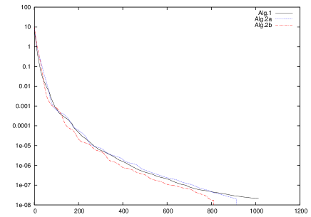
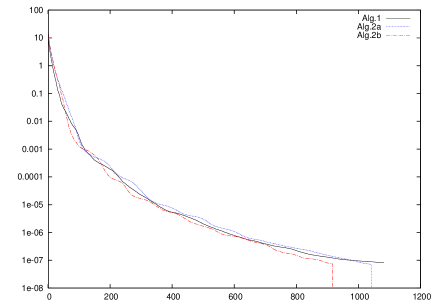
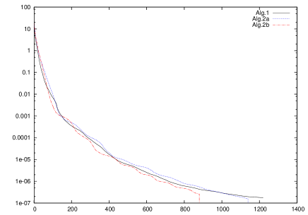
Figure 1: Convergence of Alg. 1 and the two variants of Alg. 2 for the first time step of the benchmark problem. The values of ${\mathcal{E}}_{{}\mathchoice{\mbox{\boldmath$\displaystyle\mathchar 290\relax$}}{\mbox{\boldmath$\textstyle\mathchar 290\relax$}}{\mbox{\boldmath$\scriptstyle\mathchar 290\relax$}}{\mbox{\boldmath$\scriptscriptstyle\mathchar 290\relax$}}}$ are rendered on the ordinate as a function of the L-BFGS-iterations on the abscissa. Top left: Spatial resolution $d_{1}=d_{2}=d_{3}=30$. Top right: Resolution $d_{1}=d_{2}=d_{3}=40$. Bottom: Resolution $d_{1}=d_{2}=d_{3}=50$. The exact solution in all cases is ${\mathcal{E}}_{{}\mathchoice{\mbox{\boldmath$\displaystyle\mathchar 290\relax$}}{\mbox{\boldmath$\textstyle\mathchar 290\relax$}}{\mbox{\boldmath$\scriptstyle\mathchar 290\relax$}}{\mbox{\boldmath$\scriptscriptstyle\mathchar 290\relax$}}}=0$.

This section conducts numerical tests of the preconditioning strategy presented in Section 4. While for large values of the stop parameter ${{}\mathchoice{\mbox{\boldmath$\displaystyle\mathchar 290\relax$}}{\mbox{\boldmath$\textstyle\mathchar 290\relax$}}{\mbox{\boldmath$\scriptstyle\mathchar 290\relax$}}{\mbox{\boldmath$\scriptscriptstyle\mathchar 290\relax$}}}_{0}$ the code usually converges after a small number of iterations, preconditioning becomes mandatory when ${{}\mathchoice{\mbox{\boldmath$\displaystyle\mathchar 290\relax$}}{\mbox{\boldmath$\textstyle\mathchar 290\relax$}}{\mbox{\boldmath$\scriptstyle\mathchar 290\relax$}}{\mbox{\boldmath$\scriptscriptstyle\mathchar 290\relax$}}}_{0}$ is chosen small. Fig 1 demonstrates that reducing ${{}\mathchoice{\mbox{\boldmath$\displaystyle\mathchar 290\relax$}}{\mbox{\boldmath$\textstyle\mathchar 290\relax$}}{\mbox{\boldmath$\scriptstyle\mathchar 290\relax$}}{\mbox{\boldmath$\scriptscriptstyle\mathchar 290\relax$}}}_{0}$ may go along with an exponential increase of the number of iterations. Simultaneously, fine properties of the physical solution may be missed when ${{}\mathchoice{\mbox{\boldmath$\displaystyle\mathchar 290\relax$}}{\mbox{\boldmath$\textstyle\mathchar 290\relax$}}{\mbox{\boldmath$\scriptstyle\mathchar 290\relax$}}{\mbox{\boldmath$\scriptscriptstyle\mathchar 290\relax$}}}_{0}$ is set too large, cf. also Table 3. The following bending problem of a 3D rod, see (Ble13, , Eqn. (27)), serves as a test problem. For given ${{}\mathchoice{\mbox{\boldmath$\displaystyle\mathchar 268\relax$}}{\mbox{\boldmath$\textstyle\mathchar 268\relax$}}{\mbox{\boldmath$\scriptstyle\mathchar 268\relax$}}{\mbox{\boldmath$\scriptscriptstyle\mathchar 268\relax$}}}(t)$ as in (50), $\textstyle\mathchar 295\relax$ at $\partial\Omega$ is prescribed by

$$g_{D}^{\mathrm{bend}}(x_{1},x_{2},x_{3},t):=\left(\begin{array}[]{c}x_{1}\\ x_{2}+\frac{2L_{1}}{{{}\mathchoice{\mbox{\boldmath$\displaystyle\mathchar 281\relax$}}{\mbox{\boldmath$\textstyle\mathchar 281\relax$}}{\mbox{\boldmath$\scriptstyle\mathchar 281\relax$}}{\mbox{\boldmath$\scriptscriptstyle\mathchar 281\relax$}}}}\Big{[}\sin\Big{(}\frac{3{{}\mathchoice{\mbox{\boldmath$\displaystyle\mathchar 281\relax$}}{\mbox{\boldmath$\textstyle\mathchar 281\relax$}}{\mbox{\boldmath$\scriptstyle\mathchar 281\relax$}}{\mbox{\boldmath$\scriptscriptstyle\mathchar 281\relax$}}}}{2}+\frac{{{}\mathchoice{\mbox{\boldmath$\displaystyle\mathchar 281\relax$}}{\mbox{\boldmath$\textstyle\mathchar 281\relax$}}{\mbox{\boldmath$\scriptstyle\mathchar 281\relax$}}{\mbox{\boldmath$\scriptscriptstyle\mathchar 281\relax$}}}}{2}\frac{x_{1}}{L_{1}}\Big{)}+1\Big{]}{{}\mathchoice{\mbox{\boldmath$\displaystyle\mathchar 268\relax$}}{\mbox{\boldmath$\textstyle\mathchar 268\relax$}}{\mbox{\boldmath$\scriptstyle\mathchar 268\relax$}}{\mbox{\boldmath$\scriptscriptstyle\mathchar 268\relax$}}}(t)\\ x_{3}\end{array}\right).$$ (51)

In order to determine the boundary conditions on $q$, let

$$R_{D}^{\mathrm{bend}}:=\mathrm{polar}(Dg_{D}^{\mathrm{bend}}F_{\mathrm{p}}^{-1}),$$

where $\mathrm{polar}(\cdot)$ is the polar decomposition, computed with the algorithm in Dongarra79 . Then set

$$q=q_{D}^{\mathrm{bend}}\mbox{ on }\partial\Omega,$$

where $R_{\mathrm{\!e}}(q_{D}^{\mathrm{bend}})=R_{D}^{\mathrm{bend}}$ and $q_{D}^{\mathrm{bend}}$ is computed from $R_{D}^{\mathrm{bend}}$ with the algorithm in Shoe85 .

Parameters (Bending problem):

$$\Omega=(0,5)\!\times\!(0,1)\!\times\!(0,2),\;t\in[0,1],\;{{}\mathchoice{\mbox{\boldmath$\displaystyle\mathchar 277\relax$}}{\mbox{\boldmath$\textstyle\mathchar 277\relax$}}{\mbox{\boldmath$\scriptstyle\mathchar 277\relax$}}{\mbox{\boldmath$\scriptscriptstyle\mathchar 277\relax$}}}={{}\mathchoice{\mbox{\boldmath$\displaystyle\mathchar 278\relax$}}{\mbox{\boldmath$\textstyle\mathchar 278\relax$}}{\mbox{\boldmath$\scriptstyle\mathchar 278\relax$}}{\mbox{\boldmath$\scriptscriptstyle\mathchar 278\relax$}}}=0.025,$$

$$\;{{}\mathchoice{\mbox{\boldmath$\displaystyle\mathchar 278\relax$}}{\mbox{\boldmath$\textstyle\mathchar 278\relax$}}{\mbox{\boldmath$\scriptstyle\mathchar 278\relax$}}{\mbox{\boldmath$\scriptscriptstyle\mathchar 278\relax$}}}_{c}=0.4,\;{{}\mathchoice{\mbox{\boldmath$\displaystyle\mathchar 278\relax$}}{\mbox{\boldmath$\textstyle\mathchar 278\relax$}}{\mbox{\boldmath$\scriptstyle\mathchar 278\relax$}}{\mbox{\boldmath$\scriptscriptstyle\mathchar 278\relax$}}}_{2}=0.02;\;{{}\mathchoice{\mbox{\boldmath$\displaystyle\mathchar 293\relax$}}{\mbox{\boldmath$\textstyle\mathchar 293\relax$}}{\mbox{\boldmath$\scriptstyle\mathchar 293\relax$}}{\mbox{\boldmath$\scriptscriptstyle\mathchar 293\relax$}}}={{}\mathchoice{\mbox{\boldmath$\displaystyle\mathchar 283\relax$}}{\mbox{\boldmath$\textstyle\mathchar 283\relax$}}{\mbox{\boldmath$\scriptstyle\mathchar 283\relax$}}{\mbox{\boldmath$\scriptscriptstyle\mathchar 283\relax$}}}_{Y}=f_{\mathrm{ext}}=0,\;M_{\mathrm{ext}}=\mathbf{0},$$

$$\mathbf{m}=(1,0,0)^{t},\;\mathbf{n}=(0,1,0)^{t},\;{{}\mathchoice{\mbox{\boldmath$\displaystyle\mathchar 268\relax$}}{\mbox{\boldmath$\textstyle\mathchar 268\relax$}}{\mbox{\boldmath$\scriptstyle\mathchar 268\relax$}}{\mbox{\boldmath$\scriptscriptstyle\mathchar 268\relax$}}}(t)=0.25*t,\;h=0.1,$$

$$\;{{}\mathchoice{\mbox{\boldmath$\displaystyle\mathchar 290\relax$}}{\mbox{\boldmath$\textstyle\mathchar 290\relax$}}{\mbox{\boldmath$\scriptstyle\mathchar 290\relax$}}{\mbox{\boldmath$\scriptscriptstyle\mathchar 290\relax$}}}=10^{-4},\;\varLambda=20,\;W_{\mathrm{c}}(q)=2{{}\mathchoice{\mbox{\boldmath$\displaystyle\mathchar 278\relax$}}{\mbox{\boldmath$\textstyle\mathchar 278\relax$}}{\mbox{\boldmath$\scriptstyle\mathchar 278\relax$}}{\mbox{\boldmath$\scriptscriptstyle\mathchar 278\relax$}}}\sum_{l=1}^{3}|\partial_{l}q|^{2},$$

$$\mbox{\it Initial values: }{{}\mathchoice{\mbox{\boldmath$\displaystyle\mathchar 295\relax$}}{\mbox{\boldmath$\textstyle\mathchar 295\relax$}}{\mbox{\boldmath$\scriptstyle\mathchar 295\relax$}}{\mbox{\boldmath$\scriptscriptstyle\mathchar 295\relax$}}}_{0}\equiv\mathbb{I},\;{{}\mathchoice{\mbox{\boldmath$\displaystyle\mathchar 276\relax$}}{\mbox{\boldmath$\textstyle\mathchar 276\relax$}}{\mbox{\boldmath$\scriptstyle\mathchar 276\relax$}}{\mbox{\boldmath$\scriptscriptstyle\mathchar 276\relax$}}}^{0}={{}\mathchoice{\mbox{\boldmath$\displaystyle\mathchar 269\relax$}}{\mbox{\boldmath$\textstyle\mathchar 269\relax$}}{\mbox{\boldmath$\scriptstyle\mathchar 269\relax$}}{\mbox{\boldmath$\scriptscriptstyle\mathchar 269\relax$}}}^{0}=0\mbox{ in }\Omega.$$

$$\mbox{\it Boundary values: }{{}\mathchoice{\mbox{\boldmath$\displaystyle\mathchar 295\relax$}}{\mbox{\boldmath$\textstyle\mathchar 295\relax$}}{\mbox{\boldmath$\scriptstyle\mathchar 295\relax$}}{\mbox{\boldmath$\scriptscriptstyle\mathchar 295\relax$}}}=g_{D}^{\mathrm{bend}},\;q=q_{D}^{\mathrm{bend}}\mbox{ on }\partial\Omega.$$

Results: ${{}\mathchoice{\mbox{\boldmath$\displaystyle\mathchar 269\relax$}}{\mbox{\boldmath$\textstyle\mathchar 269\relax$}}{\mbox{\boldmath$\scriptstyle\mathchar 269\relax$}}{\mbox{\boldmath$\scriptscriptstyle\mathchar 269\relax$}}}(x,t)=\sin(\frac{{{}\mathchoice{\mbox{\boldmath$\displaystyle\mathchar 281\relax$}}{\mbox{\boldmath$\textstyle\mathchar 281\relax$}}{\mbox{\boldmath$\scriptstyle\mathchar 281\relax$}}{\mbox{\boldmath$\scriptscriptstyle\mathchar 281\relax$}}}}{2}\frac{x_{1}}{L_{1}}){{}\mathchoice{\mbox{\boldmath$\displaystyle\mathchar 268\relax$}}{\mbox{\boldmath$\textstyle\mathchar 268\relax$}}{\mbox{\boldmath$\scriptstyle\mathchar 268\relax$}}{\mbox{\boldmath$\scriptscriptstyle\mathchar 268\relax$}}}(t)$, $q=(1,0,0,q_{4})$, $U_{\mathrm{\!e}}=\mathbb{I}$,
           $W_{\mathrm{st}}\equiv 0$, ${{}\mathchoice{\mbox{\boldmath$\displaystyle\mathchar 295\relax$}}{\mbox{\boldmath$\textstyle\mathchar 295\relax$}}{\mbox{\boldmath$\scriptstyle\mathchar 295\relax$}}{\mbox{\boldmath$\scriptscriptstyle\mathchar 295\relax$}}}=g_{D}^{\mathrm{bend}}$ in $\overline{\Omega}$.

Table 4 compares the numerical costs for solving the first time step of the bending problem with the original L-BFGS-algorithm (where $H^{0}_{k}$ is defined by (43)) and with the preconditioned two-step L-BFGS-algorithm of Section 4 when ${{}\mathchoice{\mbox{\boldmath$\displaystyle\mathchar 290\relax$}}{\mbox{\boldmath$\textstyle\mathchar 290\relax$}}{\mbox{\boldmath$\scriptstyle\mathchar 290\relax$}}{\mbox{\boldmath$\scriptscriptstyle\mathchar 290\relax$}}}_{0}:=10^{-11}$. Again, this behavior is typical. In our numerical tests, the two-step preconditioner leads to a significant speed-up, often accompanied with increased precision.

6 Discussion

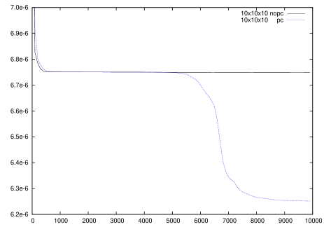
Figure 2: The progression of ${\mathcal{E}}_{{}\mathchoice{\mbox{\boldmath$\displaystyle\mathchar 290\relax$}}{\mbox{\boldmath$\textstyle\mathchar 290\relax$}}{\mbox{\boldmath$\scriptstyle\mathchar 290\relax$}}{\mbox{\boldmath$\scriptscriptstyle\mathchar 290\relax$}}}$ (ordinate) for the first $10000$ L-BFGS-iterations (abscissa) of the original L-BFGS method (black) and the preconditioned L-BFGS method (blue) for $d_{1}\!=\!d_{2}\!=\!d_{3}\!=\!10$, ${{}\mathchoice{\mbox{\boldmath$\displaystyle\mathchar 290\relax$}}{\mbox{\boldmath$\textstyle\mathchar 290\relax$}}{\mbox{\boldmath$\scriptstyle\mathchar 290\relax$}}{\mbox{\boldmath$\scriptscriptstyle\mathchar 290\relax$}}}_{0}\!=\!10^{-11}$, and the first time step of the bending problem. As can be seen, even the preconditioned algorithm requires many iterations to overcome local minima of the energy.

In this paper, a parameterization by quaternions is applied to a strongly non-linear finite-strain Cosserat model of plastic materials, possibly with microstructure. Despite increased memory requirements, in the conducted numerical tests the quaternion-based algorithm needed less iterations and converged faster. As main result, a novel two-level preconditioning scheme is proposed that exploits the physical properties of the Cosserat model. The preconditioner solves a simplified problem for $R_{\mathrm{\!e}}$ with fixed $({{}\mathchoice{\mbox{\boldmath$\displaystyle\mathchar 295\relax$}}{\mbox{\boldmath$\textstyle\mathchar 295\relax$}}{\mbox{\boldmath$\scriptstyle\mathchar 295\relax$}}{\mbox{\boldmath$\scriptscriptstyle\mathchar 295\relax$}}},{{}\mathchoice{\mbox{\boldmath$\displaystyle\mathchar 269\relax$}}{\mbox{\boldmath$\textstyle\mathchar 269\relax$}}{\mbox{\boldmath$\scriptstyle\mathchar 269\relax$}}{\mbox{\boldmath$\scriptscriptstyle\mathchar 269\relax$}}})$ which represents the most complicated step in computing a global minimizer of ${\mathcal{E}}_{{}\mathchoice{\mbox{\boldmath$\displaystyle\mathchar 290\relax$}}{\mbox{\boldmath$\textstyle\mathchar 290\relax$}}{\mbox{\boldmath$\scriptstyle\mathchar 290\relax$}}{\mbox{\boldmath$\scriptscriptstyle\mathchar 290\relax$}}}$. Note that the degrees of freedom in the micro-rotations are responsible for the occurrence of a large number of local minima. With this reasonably good guess for $R_{\mathrm{\!e}}$, the preconditioned algorithm is eventually able to succeed to a global minimizer. The preconditioning strategy is compatible with the L-BFGS update scheme and can be regarded as a non-linear preconditioning technique. Numerical tests support that this scheme significantly reduces the algorithmic costs and is essential to computing the physical solution when high precision is required. Similar two-step L-BFGS-algorithms may also be applicable to other classes of problems that depend in an un-symmetrical way on its variables. Fig. 2 documents a further important numerical feature: Since the energy landscape of ${\mathcal{E}}_{{}\mathchoice{\mbox{\boldmath$\displaystyle\mathchar 290\relax$}}{\mbox{\boldmath$\textstyle\mathchar 290\relax$}}{\mbox{\boldmath$\scriptstyle\mathchar 290\relax$}}{\mbox{\boldmath$\scriptscriptstyle\mathchar 290\relax$}}}$ consists of many flat plateaus, the L-BFGS-scheme stagnates for a long time with each step only slightly decreasing ${\mathcal{E}}_{{}\mathchoice{\mbox{\boldmath$\displaystyle\mathchar 290\relax$}}{\mbox{\boldmath$\textstyle\mathchar 290\relax$}}{\mbox{\boldmath$\scriptstyle\mathchar 290\relax$}}{\mbox{\boldmath$\scriptscriptstyle\mathchar 290\relax$}}}$. It is unknown if and when an iteration significantly decreases the energy. When ${{}\mathchoice{\mbox{\boldmath$\displaystyle\mathchar 290\relax$}}{\mbox{\boldmath$\textstyle\mathchar 290\relax$}}{\mbox{\boldmath$\scriptstyle\mathchar 290\relax$}}{\mbox{\boldmath$\scriptscriptstyle\mathchar 290\relax$}}}_{0}$ in (39) is taken too large, the algorithm may wrongly interpret this stagnation as convergence. It would be desirable to have analytic results on the choice of ${{}\mathchoice{\mbox{\boldmath$\displaystyle\mathchar 290\relax$}}{\mbox{\boldmath$\textstyle\mathchar 290\relax$}}{\mbox{\boldmath$\scriptstyle\mathchar 290\relax$}}{\mbox{\boldmath$\scriptscriptstyle\mathchar 290\relax$}}}_{0}$, or even better an algorithm that is capable to prevent this stagnation period. Finally, it may be desirable to develop a specialized L-BFGS algorithm that restricts the variations of the functional w.r.t. certain variables to the tangent space.

We address the above generalizations and enrichments of the numerical model presented in this study, together with the analysis of the more general case of gradient-type plasticity and hysteretic response under general loading, Gurtin02 ; CHM2002 ; bardellaJMPS , to future work. Additional future research lines will be devoted to applying the current Cosserat model to bending-dominated lattices with plastic behavior which exhibit arbitrarily large size effects and consist, e.g., of cubical modules/particles connected by deformable links or Sarrus linkages tessellating triangular lattice structures ZMP17 . Physical models of such systems will be fabricated through AM in ductile materials, pentamode . These mockups will be laboratory-tested in order to validate the accuracy of numerical simulations and to demonstrate the presence of size effects that cannot be described through classical continuum or homogenization theories. Recent results revealing metamaterial-type behaviors of the above systems, which are related to auxetic response ZMP17 and/or high strength effects induced by bending and twisting of the material, will be extended to the plastic regime on accounting for a ductile response of the background material.

Figure captions

Parameterizations	Resolution	No.	No.	Memory
	$(d_{1},d_{2},d_{3})$	Unknowns	Nodes	(MB)
Euler angles	$(32,32,32)$	$214683$	$35937$	$1.64$
Euler angles	$(64,64,64)$	$1774907$	$274625$	$13.5$
Euler angles	$(128,128,128)$	$14436987$	$2146689$	$110$
Euler angles	$(256,256,256)$	$116462843$	$16974593$	$889$
Quaternions	$(32,32,32)$	$244476$	$35937$	$1.86$
Quaternions	$(64,64,64)$	$2024956$	$274625$	$15.4$
Quaternions	$(128,128,128)$	$16485372$	$2146689$	$126$
Quaternions	$(256,256,256)$	$133044220$	$16974593$	$1015$

Table 1: Comparison between the parameterizations by Euler angles (7) and by quaternions (12). ’No. Unknowns’ is the total number of unknowns in the discrete model, ’Memory’ the total memory for storing the data in case of $64$ bit precision, ’No Nodes’ the total number of discretization points in the finite difference mesh.

Algorithm	$10\times 10\times 10$	$30\times 30\times 30$	$50\times 50\times 50$	$70\times 70\times 70$
Alg. 1	$359\;(0.91$s$)$	$1022\;(119$s$)$	$1228\;(723$s$)$	$1383\;(2040$s$)$
Alg. 2a	$332\;(0.93$s$)$	$919\;(107$s$)$	$1150\;(650$s$)$	$1239\;(1973$s$)$
Alg. 2b	$299\;(0.89$s$)$	$812\;(81$s$)$	$891\;(541$s$)$	$1119\;(1370$s$)$

Table 2: Averaged number of iterations for Alg. 1 and Alg. 2a/b for different spatial resolutions $d_{1}\!\times\!d_{2}\!\times\!d_{3}$ and the benchmark problem over the time interval $[0,1]$. Averaged computation times are in brackets.

Algorithm	$10\times 10\times 10$	$30\times 30\times 30$	$50\times 50\times 50$	$70\times 70\times 70$
Alg. 2a	$8.42\cdot 10^{-9}$	$4.64\cdot 10^{-8}$	$5.01\cdot 10^{-7}$	$1.04\cdot 10^{-6}$
(${{}\mathchoice{\mbox{\boldmath$\displaystyle\mathchar 290\relax$}}{\mbox{\boldmath$\textstyle\mathchar 290\relax$}}{\mbox{\boldmath$\scriptstyle\mathchar 290\relax$}}{\mbox{\boldmath$\scriptscriptstyle\mathchar 290\relax$}}}_{0}=10^{-7}$)
Alg. 2a	$8.21\cdot 10^{-14}$	$4.81\cdot 10^{-12}$	$1.22\cdot 10^{-12}$	$3.05\cdot 10^{-11}$
( ${{}\mathchoice{\mbox{\boldmath$\displaystyle\mathchar 290\relax$}}{\mbox{\boldmath$\textstyle\mathchar 290\relax$}}{\mbox{\boldmath$\scriptstyle\mathchar 290\relax$}}{\mbox{\boldmath$\scriptscriptstyle\mathchar 290\relax$}}}_{0}=10^{-9}$)

Table 3: Value of $\max\limits_{t\in[0,1]}\int\limits_{\Omega}\Lambda(|q(x,t)|^{2}-1)^{2}\,\mathrm{d}x$ for different spatial resolutions, two stop values (cf. Eqn. (39)), and Alg. 2a.

Resolution	Iterations	Iterations	Time	Time
	L-BFGS	pc-L-BFGS	L-BFGS	pc-L-BFGS
$10\times 10\times 10$	$22166995$	$41/13554468$	$383\mbox{min}\;28$s	$234\mbox{min}\;37$s
$20\times 20\times 20$	$15773252$	$133/162642$	$2656\mbox{min}\;31$s	$24\mbox{min}\;56$s
$30\times 30\times 30$	$62300391$	$269/229012$	$41131\mbox{min}\;17$s	$128\mbox{min}57$s

Table 4: The first time step of the bending problem for the original (’L-BFGS’) and the preconditioned (’pc-L-BFGS’) scheme in comparison for ${{}\mathchoice{\mbox{\boldmath$\displaystyle\mathchar 290\relax$}}{\mbox{\boldmath$\textstyle\mathchar 290\relax$}}{\mbox{\boldmath$\scriptstyle\mathchar 290\relax$}}{\mbox{\boldmath$\scriptscriptstyle\mathchar 290\relax$}}}_{0}=10^{-11}$. For the preconditioned scheme, both predictor and corrector iterations are listed. ’Time’ is the total computation time for the solution of one time step.

Appendix - List of symbols

=              =                                                                 =              =
¿$A\!:\!B$ ¿tensor product of $A$, $B$, below (16)
¿$\mathbf{u}\!\cdot\!\mathbf{v}$ ¿inner product of $\mathbf{u}$, $\mathbf{v}\in\mathbb{R}^{3}$
¿$\mathop{\mathrm{sym}}({{}\mathchoice{\mbox{\boldmath$\displaystyle\mathchar 283\relax$}}{\mbox{\boldmath$\textstyle\mathchar 283\relax$}}{\mbox{\boldmath$\scriptstyle\mathchar 283\relax$}}{\mbox{\boldmath$\scriptscriptstyle\mathchar 283\relax$}}})$ ¿symmetric part of a tensor $\textstyle\mathchar 283\relax$, (2)
¿$\operatorname{skw}({{}\mathchoice{\mbox{\boldmath$\displaystyle\mathchar 283\relax$}}{\mbox{\boldmath$\textstyle\mathchar 283\relax$}}{\mbox{\boldmath$\scriptstyle\mathchar 283\relax$}}{\mbox{\boldmath$\scriptscriptstyle\mathchar 283\relax$}}})$¿skew-symmetric part of $\textstyle\mathchar 283\relax$, (2)
¿$\mbox{tr}\,({{}\mathchoice{\mbox{\boldmath$\displaystyle\mathchar 283\relax$}}{\mbox{\boldmath$\textstyle\mathchar 283\relax$}}{\mbox{\boldmath$\scriptstyle\mathchar 283\relax$}}{\mbox{\boldmath$\scriptscriptstyle\mathchar 283\relax$}}})$ ¿trace of tensor $\textstyle\mathchar 283\relax$
¿${{}\mathchoice{\mbox{\boldmath$\displaystyle\mathchar 283\relax$}}{\mbox{\boldmath$\textstyle\mathchar 283\relax$}}{\mbox{\boldmath$\scriptstyle\mathchar 283\relax$}}{\mbox{\boldmath$\scriptscriptstyle\mathchar 283\relax$}}}^{t}$ ¿transpose of $\textstyle\mathchar 283\relax$; $R^{t}\!=\!R^{-1}$ for $R\!\in\!\mathcal{SO}(3)$
¿$\|\cdot\|$ ¿Frobenius matrix norm, (2)
¿$|\cdot|$ ¿Euclidean vector norm in $\mathbb{R}^{4}$, (26)
¿$\Omega\subset\mathbb{R}^{3}$ ¿reference domain, undeformed solid
¿$(x,t)$ ¿space and time coordinates
¿$\textstyle\mathchar 295\relax$ ¿deformation vector of the solid, (13)
¿$F\!=\!D{{}\mathchoice{\mbox{\boldmath$\displaystyle\mathchar 295\relax$}}{\mbox{\boldmath$\textstyle\mathchar 295\relax$}}{\mbox{\boldmath$\scriptstyle\mathchar 295\relax$}}{\mbox{\boldmath$\scriptscriptstyle\mathchar 295\relax$}}}$ ¿deformation tensor, (13)
¿$F_{\mathrm{e}}$ ¿elasticity tensor, (13)
¿$F_{\mathrm{p}}$ ¿plasticity tensor, (13)
¿$R_{\mathrm{\!e}}$ ¿rotation tensor, (7), (12), (13)
¿$U_{\mathrm{\!e}}$ ¿(right) stretching tensor, (13)
¿$K_{\mathrm{\!e}}$ ¿(right) curvature tensor, (32)
¿$\mathbb{I}$ ¿identity tensor, $(\mathbb{I})_{kl}=({{}\mathchoice{\mbox{\boldmath$\displaystyle\mathchar 270\relax$}}{\mbox{\boldmath$\textstyle\mathchar 270\relax$}}{\mbox{\boldmath$\scriptstyle\mathchar 270\relax$}}{\mbox{\boldmath$\scriptscriptstyle\mathchar 270\relax$}}}_{kl})_{kl}$, (20)
¿$\textstyle\mathchar 267\relax$ ¿Euler angle parameterization of $R_{\mathrm{\!e}}$, (7)
¿$\textstyle\mathchar 269\relax$ ¿single-slip parameterization of $F_{\mathrm{p}}$, (20)
¿$q$ ¿Quaternion parameterization of $R_{\mathrm{\!e}}$, (12)
¿$q_{D}$ ¿Dirichlet boundary values of $q$, (18)
¿${\mathcal{E}}$ ¿mechanical energy, (23)
¿$h>0$ ¿discrete (fixed) time step, (23)
¿${{}\mathchoice{\mbox{\boldmath$\displaystyle\mathchar 269\relax$}}{\mbox{\boldmath$\textstyle\mathchar 269\relax$}}{\mbox{\boldmath$\scriptstyle\mathchar 269\relax$}}{\mbox{\boldmath$\scriptscriptstyle\mathchar 269\relax$}}}^{0}$ ¿values of $\textstyle\mathchar 269\relax$ at old time $t$, (22)
¿${{}\mathchoice{\mbox{\boldmath$\displaystyle\mathchar 276\relax$}}{\mbox{\boldmath$\textstyle\mathchar 276\relax$}}{\mbox{\boldmath$\scriptstyle\mathchar 276\relax$}}{\mbox{\boldmath$\scriptscriptstyle\mathchar 276\relax$}}}^{0}$ ¿values of $\textstyle\mathchar 276\relax$ at old time $t$, (22)
¿$\textstyle\mathchar 276\relax$ ¿ dislocation density, (22)
¿$V({{}\mathchoice{\mbox{\boldmath$\displaystyle\mathchar 276\relax$}}{\mbox{\boldmath$\textstyle\mathchar 276\relax$}}{\mbox{\boldmath$\scriptstyle\mathchar 276\relax$}}{\mbox{\boldmath$\scriptscriptstyle\mathchar 276\relax$}}})$ ¿dislocation energy, (16)
¿$W_{\mathrm{st}}$ ¿stretching energy, (2)
¿$W_{\mathrm{c}}$ ¿curvature energy, (15)
¿$X$ ¿back stress (dual variable to $F_{\mathrm{p}}$), (19),
¿$\textstyle\mathchar 280\relax$ ¿hardening (dual variable to $\textstyle\mathchar 276\relax$), (19)
¿$f_{\mathrm{ext}}$ ¿external volume forces, (23)
¿$M_{\mathrm{ext}}$ ¿external volume couples, (23)
¿${{}\mathchoice{\mbox{\boldmath$\displaystyle\mathchar 283\relax$}}{\mbox{\boldmath$\textstyle\mathchar 283\relax$}}{\mbox{\boldmath$\scriptstyle\mathchar 283\relax$}}{\mbox{\boldmath$\scriptscriptstyle\mathchar 283\relax$}}}_{Y}$ ¿yield stress, (23)
¿$Q^{*}$ ¿dissipated energy, (21)
¿$\mathbf{m}$ ¿slip vector, (20)
¿$\mathbf{n}$ ¿slip normal, (20)
¿${{}\mathchoice{\mbox{\boldmath$\displaystyle\mathchar 293\relax$}}{\mbox{\boldmath$\textstyle\mathchar 293\relax$}}{\mbox{\boldmath$\scriptstyle\mathchar 293\relax$}}{\mbox{\boldmath$\scriptscriptstyle\mathchar 293\relax$}}}>0$ ¿dislocation energy constant, (23)
¿$g_{{}_{D}}$ ¿Dirichlet boundary values of $\textstyle\mathchar 295\relax$, (18)
¿${{}\mathchoice{\mbox{\boldmath$\displaystyle\mathchar 290\relax$}}{\mbox{\boldmath$\textstyle\mathchar 290\relax$}}{\mbox{\boldmath$\scriptstyle\mathchar 290\relax$}}{\mbox{\boldmath$\scriptscriptstyle\mathchar 290\relax$}}}>0$ ¿regularization of $|\cdot|$, Remark 1
¿$\Lambda>0$ ¿Lagrange parameter to $|q|^{2}=1$, (23)
¿$\textstyle\mathchar 277\relax$, $\textstyle\mathchar 278\relax$ ¿ Lamé parameters, (2)
¿${{}\mathchoice{\mbox{\boldmath$\displaystyle\mathchar 278\relax$}}{\mbox{\boldmath$\textstyle\mathchar 278\relax$}}{\mbox{\boldmath$\scriptstyle\mathchar 278\relax$}}{\mbox{\boldmath$\scriptscriptstyle\mathchar 278\relax$}}}_{c}$ ¿Cosserat couple modulus, (2)
¿$L_{c}$ ¿ internal length scale, (15)
¿${{}\mathchoice{\mbox{\boldmath$\displaystyle\mathchar 278\relax$}}{\mbox{\boldmath$\textstyle\mathchar 278\relax$}}{\mbox{\boldmath$\scriptstyle\mathchar 278\relax$}}{\mbox{\boldmath$\scriptscriptstyle\mathchar 278\relax$}}}_{2}$ ¿ parameter $\textstyle\mathchar 278\relax$ scaled by $L_{c}^{2}$, (15)
¿$d_{1},\!d_{2},\!d_{3}$ ¿spatial resolution, (44)
¿${{}\mathchoice{\mbox{\boldmath$\displaystyle\mathchar 273\relax$}}{\mbox{\boldmath$\textstyle\mathchar 273\relax$}}{\mbox{\boldmath$\scriptstyle\mathchar 273\relax$}}{\mbox{\boldmath$\scriptscriptstyle\mathchar 273\relax$}}}_{1}\!,\!{{}\mathchoice{\mbox{\boldmath$\displaystyle\mathchar 273\relax$}}{\mbox{\boldmath$\textstyle\mathchar 273\relax$}}{\mbox{\boldmath$\scriptstyle\mathchar 273\relax$}}{\mbox{\boldmath$\scriptscriptstyle\mathchar 273\relax$}}}_{2},\!\!{{}\mathchoice{\mbox{\boldmath$\displaystyle\mathchar 273\relax$}}{\mbox{\boldmath$\textstyle\mathchar 273\relax$}}{\mbox{\boldmath$\scriptstyle\mathchar 273\relax$}}{\mbox{\boldmath$\scriptscriptstyle\mathchar 273\relax$}}}_{3}$ ¿points on the numerical mesh, (45)
¿$N_{IJK}$ ¿discrete numerical weights, (44)
¿${{}\mathchoice{\mbox{\boldmath$\displaystyle\mathchar 268\relax$}}{\mbox{\boldmath$\textstyle\mathchar 268\relax$}}{\mbox{\boldmath$\scriptstyle\mathchar 268\relax$}}{\mbox{\boldmath$\scriptscriptstyle\mathchar 268\relax$}}}(t)$ ¿deformation parameter, (50), (51).

Compliance with Ethical Standards

The authors declare that they have no conflict of interest.