Local Bures-Wasserstein Transport: A Practical and Fast Mapping Approximation

Abstract

Optimal transport (OT)-based methods have a wide range of applications and have attracted a tremendous amount of attention in recent years. However, most of the computational approaches of OT do not learn the underlying transport map. Although some algorithms have been proposed to learn this map, they rely on kernel-based methods, which makes them prohibitively slow when the number of samples increases. Here, we propose a way to learn an approximate transport map and a parametric approximation of the Wasserstein barycenter. We build an approximated transport mapping by leveraging the closed-form of Gaussian (Bures-Wasserstein) transport; we compute local transport plans between matched pairs of the Gaussian components of each density. The learned map generalizes to out-of-sample examples. We provide experimental results on simulated and real data, comparing our proposed method with other mapping estimation algorithms. Preliminary experiments suggest that our proposed method is not only faster, with a factor 80 overall running time, but it also requires fewer components than state-of-the-art methods to recover the support of the barycenter. From a practical standpoint, it is straightforward to implement and can be used with a conventional machine learning pipeline.

1 Introduction

In recent years, Optimal Transport-based algorithms (OT)[24] are increasingly attracting the machine learning community. OT leverages useful information about the nature of a problem by encoding the geometry of the underlying space through a cost metric. As OT measures distances between probability distributions, it is generally used as an optimization loss [1, 12, 14, 29]. OT aims at finding a probabilistic matrix that couples two distributions; this matrix is also called a transportation matrix. However, we can only use this matrix with the data used to learn it. Thus, one has to recompute an OT problem to handle new samples. Hence, it is prohibitive for some applications where the OT problem is not used as a distance to be minimized, for instance, transport out-of-sample data into a fixed distribution [7]. Another critical application is computing a weighted mean in a Wasserstein space. This weighted mean is known as the Wasserstein barycenter, which has numerous applications in unsupervised learning. It is used to represent the input data [26], to cluster densities [31], to analyze shapes [25], to build fair classifiers [10], among other applications.

To handle unseen data, [23] proposes to learn a transport map. However, this approach relies on kernel-based methods, which makes it slow when the number of samples increases. To approximate the barycenter, [5] proposes to decompose the input data into sums of radial basis functions and perform partial transport between matched pairs of functions coming from each distribution. However, it is not clear what is the influence of noise in this approximation as it handles the positive and negative parts of the data independently. Additionally, the extension of this approach to out-of-sample data is not explored.

Contributions.

We propose to use a local approximation of the Gaussian (Bures-Wasserstein) transport to speed up learning mappings and barycenters that can be applied to unseen data. This approach assumes that the densities involved in the transport problem are highly concentrated in a few clusters/components. This idea is reminiscent of the computation of barycenters by partial transport [5]. The key point is to express each density as a mixture of Gaussians; contrary to [5], it is no longer necessary to split the input data into its positive and negative parts. Then, we can use the means and covariances of these Gaussian functions to approximate the transport map as well as the barycenter. To do so, we use these means as a new spatial reference. Then, we match pairs of means of different distributions and solve OT problems for each matched pair.

The proposed method unifies the learning of the barycenter and transport map. We provide some empirical evidence for the usefulness of our approach in two tasks: i) interpolating of clouds of points, and ii) building fair classifiers. Through experiments on public datasets, we show the improvements brought by our scheme with respect to standard mapping estimation methods. Our approach can be easily implemented and combined with conventional machine learning pipelines.

Notation.

Column vectors are denoted as bold lower-case, e.g, $\mathbf{a}$. Matrices are written using bold capital letters, e.g., $\mathbf{A}$. Let $\|\cdot\|_{F}$ be the Frobenius norm of a matrix, $\mathop{\rm Tr}(\cdot)$ is the trace of a matrix, and $\mathbf{A}^{\mathsf{T}}$ is the transpose of $\mathbf{A}$. We denote the $(m-1)$-dimensional probability simplex by $\Delta^{m}\coloneqq\{\mathbf{y}\in\mathbb{R}_{+}^{m}:\|\mathbf{y}\|_{1}=1\}$. Let $n$ be the number of data points and $[n]$ denotes $\{1,\ldots,n\}$.

2 Background: Gaussian optimal transport

We will restrict ourselves to the discrete setting (i.e., histograms); thus, $\mu\in\Delta^{p}$ and $\nu\in\Delta^{q}$. The cost matrix $\mathbf{C}\in\mathbb{R}^{p\times q}$ represents the cost function (e.g., the squared Euclidean distance), which contains the cost of transportation between any two locations in the discretized grid. The OT distance between two histograms $W(\mu,\nu)$ is the solution of the discretized Monge-Kantorovich problem [30]:

$$W^{2}(\mu,\nu)=\min_{\mathbf{T}\in\Pi(\mu,\nu)}\mathop{\rm Tr}(\mathbf{T}^{\mathsf{T}}\,\mathbf{C}),$$ (1)

where $\mathbf{T}:\mathbb{R}^{p}\rightarrow\mathbb{R}^{q}$ is the transport plan, $\Pi(\mu,\nu)$ denotes the set of admissible couplings between $\mu$ and $\nu$, that is, the set of matrices with rows summing to $\mu$ and columns to $\nu$.

However, computing Eq.(1) for other distributions than Gaussians requires to solve a linear programming problem that grows at least $O(p^{3}\log p)$ [24] for histograms of dimension $p$. We can constrain the entropy of the transport plan $\mathbf{T}$ to alleviate this issue [8].

Bures-Wasserstein transport.

The OT distance in Eq.(1) can be calculated in closed-form when $\mu$ and $\nu$ are Gaussians measures, as demonstrated by [15] and discussed by [28]. This corresponds to the Bures-Wasserstein distance [3] between $\mu\sim\mathcal{N}(\mathbf{m}_{1},\mathbf{\Sigma}_{1})$ and $\nu\sim\mathcal{N}(\mathbf{m}_{2},\mathbf{\Sigma}_{2})$:

$$W_{2}^{2}(\mu,\nu)=\|\mathbf{m}_{1}-\mathbf{m}_{2}\|_{2}^{2}+\mathop{\rm Tr}(\mathbf{\Sigma}_{1}+\mathbf{\Sigma}_{2})-2\,\mathop{\rm Tr}\left[\left(\mathbf{\Sigma}_{1}^{1/2}\,\mathbf{\Sigma}_{2}\,\mathbf{\Sigma}_{1}^{1/2}\right)^{1/2}\right],$$ (2)

where $\mathbf{m}_{i}\in\mathbb{R}^{p}$ and $\mathbf{\Sigma}_{i}\in\mathbb{R}_{+}^{p\times p}$ for $i\in[2]$ are the mean vectors and the covariance matrices, respectively. $W_{2}^{2}(\cdot,\cdot)$ uses the squared Euclidean distance as transport cost. For zero-mean Gaussian random variables, the Wasserstein distance reduces to Frobenius of the covariance roots [18], and the transport map is:

$$\mathbf{T}_{\mathbf{\Sigma}_{1}}^{\mathbf{\Sigma}_{2}}=\mathbf{\Sigma}_{1}^{-1/2}\,\left(\mathbf{\Sigma}_{1}^{1/2}\mathbf{\Sigma}_{2}\,\mathbf{\Sigma}_{1}^{1/2}\right)^{1/2}\mathbf{\Sigma}_{1}^{-1/2},$$ (3)

where $\mathbf{T}_{\mathbf{\Sigma}_{1}}^{\mathbf{\Sigma}_{2}}$ is the transport map from $\mathbf{\Sigma}_{1}$ to $\mathbf{\Sigma}_{2}$. In general, the Gaussian transport $\mathbf{T}:\mathbb{R}^{p}\rightarrow\mathbb{R}^{p}$ is

$$\mathbf{T}(\mathbf{x})=\mathbf{m}_{2}+\mathbf{T}_{\mathbf{\Sigma}_{1}}^{\mathbf{\Sigma}_{2}}(\mathbf{x}-\mathbf{m}_{1}).$$ (4)

Bures-Wasserstein barycenter.

The Wasserstein barycenter problem attempts to summarize a collection of probability distributions by taking their weighted average with respect to the Wasserstein metric. In particular, the Wasserstein barycenter of $l$ Normal distributions $\mathcal{N}(\mathbf{m}_{0},\mathbf{\Sigma}_{0}),\ldots,\mathcal{N}(\mathbf{m}_{l},\mathbf{\Sigma}_{l})$, with weights $\boldsymbol{\lambda}\in\Delta^{l}$ is the solution of the minimization problem

$$\min\limits_{\bar{\mathbf{m}}\in\mathbb{R}^{p},\bar{\mathbf{\Sigma}}\in\mathbb{S}_{+}}\sum\limits_{i=1}^{l}\boldsymbol{\lambda}_{i}\,W_{2}^{2}(\mathcal{N}(\bar{\mathbf{m}},\bar{\mathbf{\Sigma}}),\mathcal{N}(\mathbf{m}_{i},\mathbf{\Sigma}_{i})).$$ (5)

The barycenter of Gaussians is still Gaussian, and its mean $\bar{\mathbf{m}}$ can be computed directly as $\bar{\mathbf{m}}=\sum_{i=0}^{l}\boldsymbol{\lambda}_{i}\,\mathbf{m}_{i}$. However, its covariance $\bar{\mathbf{\Sigma}}$ is the solution of the following matrix equation

$$\bar{\mathbf{\Sigma}}=\sum_{i=1}^{l}\boldsymbol{\lambda}_{i}\left(\bar{\mathbf{\Sigma}}^{1/2}\,\mathbf{\Sigma}_{i}\,\bar{\mathbf{\Sigma}}^{1/2}\right)^{1/2},$$ (6)

which has not a closed-form solution for $l>2$.

Algorithm 1 Barycenter of covariances [18]

1:$\mathbf{\Sigma}_{i}\in\mathbb{R}^{p\times p}$, $i\in[l]$, and $\boldsymbol{\lambda}\in\Delta^{l}$.

2:while Stopping criterion is not met do

3:    Compute $\mathbf{T}_{\mathbf{\Sigma}_{i}}^{\bar{\mathbf{\Sigma}}^{t}}$ for each $i\in[l]$ using Eq.(3)

4:    Linear averaging, $\mathbf{T}=\sum\limits_{i=1}^{l}\boldsymbol{\lambda}_{i}\,\mathbf{T}_{\mathbf{\Sigma}_{i}}^{\hat{\mathbf{\Sigma}}^{t}}$

5:    Retraction, $\bar{\mathbf{\Sigma}}^{t+1}=\mathbf{T}\bar{\mathbf{\Sigma}}^{t}\mathbf{T}$

6:    Set $t=t+1$

7:end while

8:return Barycenter $\bar{\mathbf{\Sigma}}^{t+1}$

The algorithm 1[18] finds a fixed point of Eq.(6). It initializes the barycenter with a positive definite matrix. Then, it lifts all observation to the tangent space at the initial guess via log map and performs a linear averaging. This average is then retracted onto the manifold via the exponential map, providing a new guess. The algorithm iterates until it reaches the stop condition (e.g., number of iterations).

3 The model

We are interested in a fast approximation of a transport map that generalizes to out-of-samples data. We assume the data lives in a low-dimensional feature space, and a few Gaussians concentrate the samples. Thus, we use mixtures of Gaussians to approximate independently the densities $\mu$ and $\nu$ involved in Eq.(1). Then, we compute the pairwise transport plans (see Eq.4) at the component level. We refer to this approach as local Bures-Wasserstein (L-BW) transport.

Gaussian Mixture Model (GMM).

We model the density $\mu$ as a weighted average of $k$ Gaussian functions, where each Gaussian or component represents a subpopulation of the data. The parameters of each component $i\in[k]$ are the mean vector $\mathbf{m}_{i}^{\mu}\in\mathbb{R}^{p}$ and covariance matrix $\mathbf{\Sigma}_{i}^{\mu}\in\mathbb{R}_{+}^{p\times p}$.

$$\mathbb{P}_{k}[\textbf{x}]=\sum_{j=1}^{k}\boldsymbol{\pi}_{j}^{\mu}\,\phi(\mathbf{x};\,\mathbf{m}_{j}^{\mu},\mathbf{\Sigma}_{j}^{\mu}),$$ (7)

where $\boldsymbol{\pi}^{\mu}\in\Delta^{k}$ is the mixing proportions, and $\phi(\cdot;\,\mathbf{m}_{j},\mathbf{\Sigma}_{j})$ denotes a $p$-dimensional Normal density with mean vector $\mathbf{m}_{j}$ and covariance matrix $\mathbf{\Sigma}_{j}$. We usually use the Expectation-Maximization (EM) algorithm to fit a GMM [13]. This algorithm alternates between estimating the probability to assign a sample $\mathbf{x}$ to component $j$, $\boldsymbol{\gamma}_{j}(\mathbf{x})\in\Delta^{k}$, and calculating the parameters of model. We denote $\delta(\mathbf{x})$ the (hard) assignment of sample $\mathbf{x}$ to a component,

$$\delta(\mathbf{x})=\mathop{\rm argmax}_{j\in[k]}\boldsymbol{\gamma}_{j}(\mathbf{x}).$$ (8)

3.1 Leveraging Bures-Wasserstein transport.

For simplicity, we describe our approach for two densities/groups. We depict how to extend it to more groups at the end of this section. Let $g\in\{a,b\}$ be the group indicator, and $\mathbf{X}^{g}\in\mathbb{R}^{|q|\times p}$ be the set of samples $\mathbf{x}$ that belong to the group $g$, where $|g|$ denotes the number of samples of group $g$.

Getting the parameters.

We aim to leverage the closed-form of the Bures-Wasserstein transport (see Eq.(4)) to learn an approximated transport map. To do so, for each $g\in\{a,b\}$, we use a $k$ mixture of Gaussians to approximate the density of $\mathbf{X}^{g}$. We use the means $\{\mathbf{m}_{i}^{g}\}_{i=1}^{k}$ as a rough approximation of the geometry. Then, we solve $k$ pairwise Bures-Wasserstein OT problems. We select pairs because the OT of Gaussians is still Gaussian, removing important geometrical information.

To select which components from each group to pair, we solve a linear allocation problem [6] of their mean vectors. In particular, we use the Hungarian algorithm [19] to match these values. This algorithm has a time complexity $O(k^{3})$, where $k\ll\min(|a|,|b|)$, and solves an OT problem for uniform distributions of the same size [24]. We set the transport cost to $\mathbf{C}_{i,j}=\|\mathbf{m}_{i}^{a}-\mathbf{m}_{j}^{b}\|^{2},\,\mathbf{C}\in\mathbb{R}^{k\times k}$. We denote $\mathbf{A}\in[0,1]^{k\times k}$ a matrix that encodes the pairwise matching of components. Thus, for $(i,j)\in[k]^{2}$, $\mathbf{A}_{i,j}=1$ if $\mathbf{m}_{i}^{a}$ match $\mathbf{m}_{j}^{b}$ and $0$ otherwise.

From now on, we rely on $\mathbf{A}$, $\left\{(\mathbf{m}_{l}^{g},\mathbf{\Sigma}_{l}^{g})\right\}_{l=1}^{k}$ and $\delta(\cdot)^{g}$ to approximate the barycenter and the transport map. The algorithm 2 presents a pseudo-code of learning these parameters.

Algorithm 2 Learning parameters of L-BW transport.

1:$\mathbf{X}^{g}\in\mathbb{R}^{|g|\times p}$ for $g\in\{a,b\}$, and a number $k$ of components.

2:Estimate parameters of GMM from samples $\mathbf{X}^{g}$: Get $\left\{(\mathbf{m}_{l}^{g},\mathbf{\Sigma}_{l}^{g})\right\}_{l=1}^{k}$ and $\delta^{g}(\cdot)$ for $g\in[a,b]$.

3:Get matching matrix $\mathbf{A}$: Set $\mathbf{C}_{i,j}=\|\mathbf{m}_{i}^{a}-\mathbf{m}_{j}^{b}\|^{2}$ for $(i,j)\in[k]^{2}$ and use the Hungarian algorithm [19].

4:return matching matrix $\mathbf{A}$, and GMM parameters $\left\{(\mathbf{m}_{l}^{g},\mathbf{\Sigma}_{l}^{g})\right\}_{l=1}^{k}$ and $\delta^{g}(\cdot)$.

We can extend this approach for a number $s$ of groups by sequentially computing one reference group and the other populations (a.k.a. one-vs-rest approach). This has a time complexity of $O(s\,k^{3})$.

Approximate a transport map.

To transport sample $\mathbf{x}$ from a distribution $a$ to another $b$, we use the algorithm 2 and apply Eq.(4) for each matched pair of components, as follows

$$\begin{split}\hat{\mathbf{T}}_{a}^{b}(\mathbf{x})&=\sum_{(i,j)\in[k]^{2}}\mathbf{A}_{i,j}\left[\mathbf{m}_{j}^{b}+\Gamma(\mathbf{x},i)\right],\\ \text{where }\Gamma(\mathbf{x},i)&=\begin{cases}\mathbf{T}_{\mathbf{\Sigma}_{i}^{a}}^{\mathbf{\Sigma}_{j}^{b}}(\mathbf{x}-\mathbf{m}_{i}^{a})&\delta^{a}(\mathbf{x})=i,\\ 0&\text{otherwise},\end{cases}\\ \end{split}$$ (9)

where $\hat{\mathbf{T}}_{a}^{b}(\mathbf{x})$ denotes the approximated transport map of $\mathbf{x}$ from the population $a$ to population $b$. In a nutshell, our algorithm performs pairwise transport between components of two distributions, $a$ and $b$. First, it uses $\delta^{a}(\mathbf{x})$ to assign a sample $\mathbf{x}$ to a $i$ subpopulation of $a$, which has parameters $\left(\mathbf{m}_{i}^{a},\mathbf{\Sigma}_{i}^{a}\right)$. Then, it matches the $i$-Gaussian of group $a$ with a $j$-component of group $b$, parametrized by $\left(\mathbf{m}_{j}^{b},\mathbf{\Sigma}_{j}^{b}\right)$. Next, it computes the Bures-Wasserstein transport of these two Gaussians. Finally, It repeats for all pairs of matched components.

Approximate a barycenter.

Algorithm 3 Approximate Barycenter

1:$\mathbf{X}^{g}\in\mathbb{R}^{|g|\times p}$ for $g\in\{a,b\}$, number $k$ of components, and weights $\boldsymbol{\lambda}\in\Delta^{2}$.

2:Estimate parameters of L-BW: use Algorithm 2

3:Initialize: $h=1$

4:for $(i,j)\in[k]^{2}$ do

5:    if $\mathbf{A}_{i,j}=1$ then

6:         $\bar{\mathbf{m}}_{h}\leftarrow$ $\boldsymbol{\lambda}_{0}\,\mathbf{m}_{i}^{a}+\boldsymbol{\lambda}_{1}\,\mathbf{m}_{j}^{b}$.

7:         $\bar{\mathbf{\Sigma}}_{h}\leftarrow$ use Algorithm 1 with $\mathbf{\Sigma}_{i}^{a}$ and $\mathbf{\Sigma}_{j}^{b}$.

8:         Set $h=h+1$

9:    end if

10:end for

11:return Parameters of barycenter $\{(\bar{\mathbf{m}}_{h},\bar{\mathbf{\Sigma}}_{h})\}_{h=1}^{k}$.

Let $c$ be the barycenter of the distributions $a$ and $b$. To approximate this barycenter, we use algorithm 2 to compute the parameters of the L-BW for $a$ and $b$. Then, we calculate the Bures-Wasserstein barycenter of every $(i,j)$-pair that satisfies the match condition. Thus, the approximated barycenter $c$ is in the space of $k$ Gaussian mixtures with parameters $\{(\bar{\mathbf{m}}_{h},\bar{\mathbf{\Sigma}}_{h})\}_{h=1}^{k}$. The algorithm 3 presents the pseudo-code of the approximate barycenter by L-BW. Fig.1 shows an illustration of this procedure.

(a) Input data.

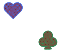
(b) Fitting GMMs.

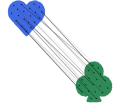
(c) Matching means.

(d) Partial transport.

Figure 1: Illustration of the working principle of the approximation of the barycenter: For each group $g$ (e.g., heart and clover), the algorithm receives a data matrix $\mathbf{X}^{g}$. It computes a GMM for each group. It uses the means of these GMMs as an approximation of the geometry. Next, it matches these means.Finally, it computes the Bures-Wasserstein barycenter for each matched pair.

4 Related work

Mapping Estimation (ME).

To extend OT-based methods to unseen data, [23] proposes an algorithm to learn the coupling and an approximation of the transport map. This optimization problem learns a transformation regularized by a transport map. However, ME relies on kernel-based methods, which usually have a time complexity of $O(n^{3})$ [2] for $n$ samples. Additionally, it requires tuning the parameters associated with each kernel and the regularization parameter.

Practical computation of the barycenter.

[5] proposes a first approach to approximate the barycenter using signal decomposition and partial transport for multiple frequency bands. However, it requires the nontrivial task of selecting the frequency bands. A second approach by [9] proposes a fast algorithm to compute the free support Wasserstein barycenter. This algorithm optimizes the locations of the barycenter and not the weights associated to the discrete measure. It uses $k$ atoms or points to constrain the support of the barycenter. It is similar to our method, as both rely on the approximation of the geometry by $k$ atoms/components. However, our approach requires fewer atoms because the covariance matrices of the Gaussian mixtures encode more geometrical information.

5 Applications

We conduct a series of experiments to highlight the versatility of Local Bures-Wasserstein (L-BW) transport. We consider two tasks: i) computing the barycenter of clouds of points and ii) building fair classifiers. Both problems use an approximation of the barycenter and the transport map.

We denote $\hat{\mathbf{T}}_{a}^{c}(\cdot)$ the learned transport map from population $a$ to $c$, where $c$ is the learned barycenter of densities $a$ and $b$. We test the learned transport map on held-out data, in a cross-validation scheme splitting the data ten times at random. Each time, we learn the barycenter and the transport map on $70\%$ of the data and apply it to the other $30\%$. Besides L-BW, we also investigate Mapping Estimation (ME) [5] with both, linear and Gaussian kernels. For the ME, we first compute the free support Wasserstein barycenter [9], and then we use ME to learn the mapping to this barycenter.

Henceforth, we refer to $k$ as the number of atoms. It represents, both, the number of components in L-BW and the number of points in the free support Wasserstein barycenter used in ME.

Technical aspects.

We used standard data processing and classification methods implemented in scikit-learn [22]. We used the POT library [11] for the convolutional Wasserstein barycenter and Mapping Estimation. We used Scipy [16] for the Hungarian algorithm. Our method is available.

5.1 Shape interpolation of clouds of points

A straightforward application of Wasserstein barycenter is the interpolation of shapes, as it relies on performing optimal transportation over geometric domains. We vary the number of atoms $k\in\{2,\ldots,100\}$ and evaluate the performance of the approximated transport map and barycenter with two measures: i) support recovery and ii) computation time. For the ME, we set the regularization parameters of the linear and Gaussian kernels to $\eta=10^{-3}$ and $\sigma=1$, respectively.

Synthetic dataset. We generated a synthetic dataset that consists of three binary $200\times 200$ images: cat, rabbit, and tooth (see Fig.6 in supp. materials). We put them in a $1200\times 1200$ square grid. We sample $\approx 10\,000$ points at random inside every silhouette. We aim to calculate the barycenter of these images given some weights $\boldsymbol{\lambda}\in\Delta^{3}$.

Quality assessment.

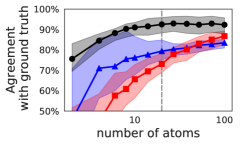
(a) Support recovery.

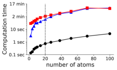
(b) Computation time.

(c)

Figure 2: Performance evaluation. The vertical dashed line denotes $k=20$. L-BW requires fewer atoms to recover the support, and it is the fastest method.

To compare the quality of the approximated barycenter, we measure its agreement proportion with ground-truth. The ground-truth is in itself a silhouette, and we build it using the convolutional 2-D Wasserstein barycenter algorithm [27], followed by binarization by thresholding. We set the threshold via the Otsu’s method [21].

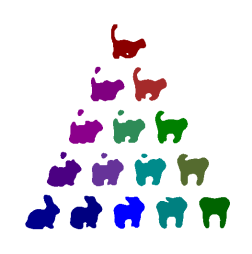
(a) Baseline: $2$-D convolutional Wasserstein[27].

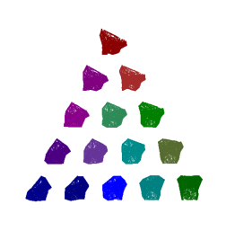
(b) ME-Linear:
$20$ atoms.

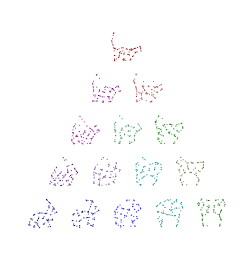
(c) ME-Gaussian:
$20$ atoms.

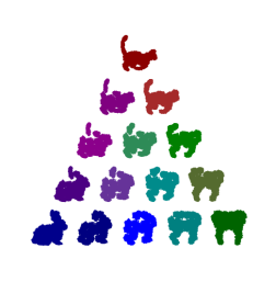
(d) L-BW: $20$ atoms.

Figure 3: Visualization of barycenters: The coordinates represent the Wasserstein simplex, which consists in all of their Wasserstein barycenters under varying weights $\boldsymbol{\lambda}\in\Delta^{3}$. Fig.3a displays the barycenters obtained by [27] after thresholding using Otsu’s method.

Fig.2a displays the support recovery of intermediate silhouettes as a function of the number of atoms. ME-based methods require five times more atoms than L-BW to improve the quality of their resulting images. L-BW has higher percentage of agreement with ground truth than ME with both linear and Gaussian kernels. It seems to reach a plateau at $k=20$, which corresponds to the best representation according to the Akaike information criterion (see Fig.7 in supp. materials).

Fig.3 shows the barycenters found by various algorithms for $k=20$ on the synthetic dataset. Fig.3a displays our ground-truth. ME-Gaussian generates barycenters that reproduce the shapes, yet it concentrates the transported samples in a few atoms. In contrast, ME-Linear does not concentrate the transported samples; however, it fails to preserve the silhouette. L-BW reproduces the transitions between inputs, and creates plausible intermediate silhouettes.

Computation time.

We measured the running time of various approaches, including both the training time and the transport time.

Fig.2b gives computation time for different methods. L-BW displays overall the lowest computation time for all atoms; on average $80$ times faster than ME-Linear. For $k<40$, ME-Linear is ten times faster than ME-Gaussian; when the number of atoms increases, this factor drops to approximately 1.5.

5.2 Demographic-parity fairness

Another application of OT is to build fair classifiers. We rely on demographic-parity, which requires that predictions of an estimator cannot reveal information about the protected class any better (up to a tolerance) than random guessing [20, 32].

We consider mixing distributions of two groups (e.g., Female and Male) via OT to produce naive fair classifiers. We modify the input data $\mathbf{X}^{g}$ by transporting each sample $\mathbf{x}$ to the barycenter $c$ of the two populations, $g\in\{a,b\}$. This is proposed in [10] for Gaussian random variables. We extend this idea to more complex distributions via L-BW, as follows

$$D\left[\mathbb{P}[\mathbf{y}|\,\hat{\mathbf{T}}_{a}^{c}(\mathbf{X}^{a});\,\theta],\mathbb{P}[\mathbf{y}|\,\hat{\mathbf{T}}_{b}^{c}(\mathbf{X}^{b});\,\theta]\right]\leq\epsilon,$$ (10)

where $\theta$ denotes the parameter of the classifier, $\mathbf{y}$ is the binary classification target, and $D(\mu,\nu)$ is a similarity measure of two distributions $\mu$ and $\nu$ (e.g., Kullback-Lieber, or Wasserstein). $\epsilon$ is the desired tolerance. This transformation of the input data is oblivious to the target; hence we do not have precise control of the tolerance $\epsilon$.

Fairness experiment.

We present an empirical study on five real-world datasets. In all classification tasks, we collect statistics concerning prediction and fairness score measure. We use nested cross-validation to set hyperparameters. Our preprocessing pipeline comprises standardization and dimensionality reduction via Principal Component Analysis (PCA). We use one-hot-encoding to handle categorical variables.

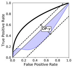
Figure 10: Visual representation of the notion of fairness: The solid black line is the ROC curve for the $\mathbf{y}$ target. The solid blue line is the ROC curve for the protected $\mathbf{z}$ label that encodes the group membership of each sample $\mathbf{x}$. DP-$\gamma$ is the maximum distance of the latter from the diagonal, which represents lack of predictability.

We use the Demographic-Parity-$\gamma$ score [20] to measure fairness. It is the maximum distance of the Receiver Operating Characteristic (ROC) curve for the group membership label from the diagonal, where zero represents an absolute lack of predictability (see Fig.10 in supp. materials). Thus, the lower the fairness score, the better. For prediction performance, we use the area under the ROC curve (AUC). This score upper bounded by $1$ and higher values mean better predictions.

Setting hyperparameters.

We vary the number of principal components $d\in\{2,4,\ldots,30\}$, and the number of atoms $k\in\{1,\ldots,10\}$ for the L-BW. We set the parameter to regularize the covariance of the GMMs to $10^{-6}$. To compute the free support Wasserstein barycenter, we set the grid $k\in\{10,20,50,100,200,300\}$. We set grid for the parameters of ME to $\eta\in\{10^{3},10^{2},10^{1},1,10\}$ and $\sigma\in\{1,10,10^{2},10^{3}\}$ for the linear and Gaussian kernels, respectively. We set weights of the barycenter to $\boldsymbol{\lambda}=[0.5,0.5]$, the new distribution should not benefit any of two populations.

Datasets.

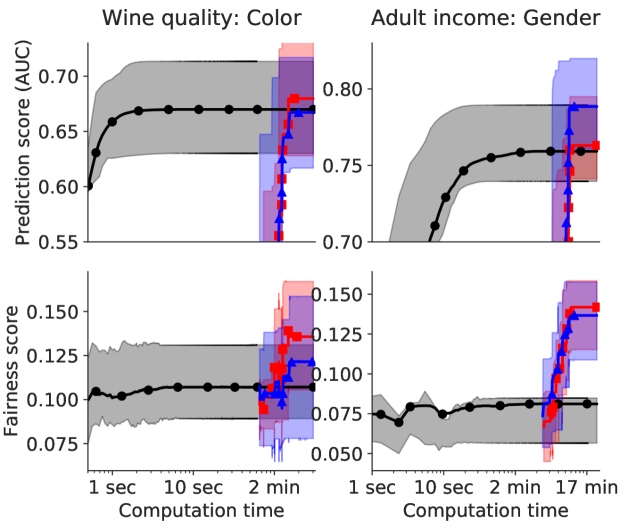
(a)

(b)

Figure 4: Computation time taken to reach a solution: Quality of the fit of a $\ell_{2}$ penalized logistic regression as a function of the computation time for a fixed number of atoms. (top) Predictive accuracy and (bottom) fairness score on held-out-data. In both datasets, L-BW obtains the best fairness score, and the same prediction score than ME-Gaussian with less computation time to reach a stable solution. The time displayed includes the computation of the barycenter and transport mapping.

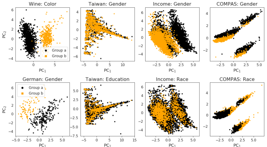
Figure 11: Visualization of the first two principal components for different datasets: We can see that for most of the datasets the groups are well separated. Training a classifier on top of this representation will lead to leak of information about the protected groups.

We investigate our approach in several binary classification problems based on four datasets from the UCI Machine Learning Repository[4]. See Fig.11 in supp. materials a visualization of the first two principal components of these datasets conditioned on the sensitive groups.

Wine quality: it contains $12$ attributes of $4\,898$ wines. Professional taste-tester provided a ranking out of $10$. The task is to predict if a wine has a rating higher or equal than $6$. The protected groups are color-based (White and Red). All explanatory variables are continuous.

German Credit Data: it contains $20$ features ($7$ numerical and $13$ categorical) related to the economic situation of $1\,000$ German applicants for loans. The aim is to predict whether or not an applicant is going to default the credit loan. The protected groups are gender-based (Female and Male).

Adult Income: it contains $14$ features concerning demographic characteristics of $45\,222$ individuals. The task is to predict whether or not a person has more than $50\,000$ as an income per year. The protected groups are education-based (Higher and Lower education) and gender-based (Male and Female).

Taiwan credit: it contains the credit information of $30\,000$ individuals $24$ features represent this information, where $9$ of them are categorical. The task is to predict customers if default payments.

COMPAS [17]: it is a collection of $10\,000$ criminal defendants screened in Broward County, Florida U.S. in $2013$ and $2014$. The features are demographics and criminal records of offenders. The task is to score an individual’s likelihood of reoffending. The protected groups are race-based (Black and White) and gender-based (Male and Female).

Fairness on a time budget.

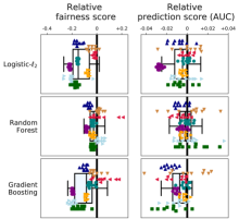
Figure 5: Impact of mixing distributions with L-BW on performance of various classifiers: The performance of classifiers after mixing sensitive groups relative to mean scores of the raw classifier (per dataset). The fairness score, the lower, the better ($<0$). The AUC, the higher, the better ($>0$). L-BW improves the fairness of logistic regression while maintaining prediction accuracy. For Gradient Bosting, L-BW reduces the fairness score at the price of decreasing accuracy. The performance of Random Forest remains the same.

We examine the impact of mixing groups on prediction time for various approximate transport map methods. We are interested in the total computation time needed to learn a model: the cost of computing the approximate representation (i.e., fitting a barycenter and a transport mapping) and of training the classifier.

Fig.4 shows the prediction accuracy as a function of the computation time for training a logistic regression with $\ell_{2}$-penalty, and it displays the mean the across folds and the percentiles $25$ and $75$. In both datasets, L-BW requires less time to converge to an estimator with a lower fairness score and displays the same predictive performance as ME-Gaussian. ME-Linear has the best classification performance in the income dataset; however, it has a more significant unfair behavior than L-BW.

Fair classifiers.

We analyze the impact of mixing groups by L-BW in various conventional classifiers: Logistic regression ($\ell_{2}$ penalty), Gradient Boosting Trees ($100$ trees), and Random Forest ($100$ trees). See Fig.13 in supp. materials for more classifiers.

Fig.5 shows the performance classifiers after mixing groups with L-BW. The performance is relative to the mean performance of the raw classifier (per dataset). The fairness score (DP-$\gamma$) of Random-Forest does not display any improvement, whereas the other classifiers present significantly better results ($\text{p}_{\text{value}}<10^{-8}$, paired Wilcoxon rank test). L-BW decreases the predictive performance of Gradient Boosting Trees to the raw classifier. This drop in accuracy is not significant for other classifiers.

6 Discussion

We proposed a fast method to compute an approximation of the barycenter and transport mapping, which can be used in out-of-sample data. Our method directly exploits highly concentrated samples in low dimensions to approximate the Wasserstein barycenter as well as the transport map. First, it approximates the training data with Gaussian mixtures. For each distribution, we fix the means of these Gaussians as the new geometrical reference. Then, we select the closest means between densities. Finally, we perform pointwise Gaussian transport between matched components. Additionally, we propose an extension of our approach to more than two densities, which has linear complexity in the number of densities. From a machine learning perspective, we can directly project held-out-data into the approximate barycenter, which makes it possible to use in standard machine learning pipelines.

We demonstrated the effectiveness of our approximation on two problems: shape interpolation of clouds of points and naive demographic-parity fair classifiers. In both problems, our method displays the fastest computation time, outperforming the ME. L-BW extends [10] to densities more complex than Gaussians. It requires fewer components to approximate the barycenter and, for most classifiers, it produces naive fair estimators while maintaining prediction accuracy. Our approach is similar to [9], as it relies on $k$ Gaussian components (atoms). Yet, our approach also takes the covariance of subpopulations into account. Experimental results confirm that this additional information benefits the support recovery of the barycenter.

However, the current framework has the following limitations: i) it assumes that the few clusters represent the densities involved, which limits its applications to low/medium dimensionality settings; ii) it assumes that the number of atoms required to approximate each distribution included in the barycenter calculation is the same, which can be problematic for some data; iii) the theoretical properties of the L-BW are out of the scope of this paper. Addressing the above limitations are new directions for future work.

7 Applications: Additional analysis

7.1 Shape interpolation of a cloud of points experiment

Figure 6: Input shapes: Cat, rabbit, and tooth. Each silhouette contains $\approx 10\,000$ points.

Figure 7: Setting the number of components: The Akaike information criterion (AIC) as a function of the number of atoms for each silhouette. $k=20$ achieves the minimum AIC for all shapes.

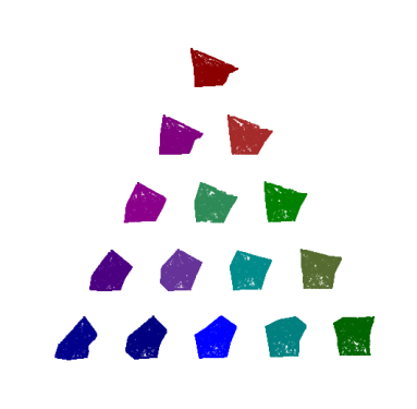
(a) ME (linear): $10$ atoms.

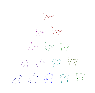
(b) ME (Gaussian): $10$ atoms.

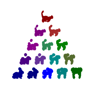
(c) L-BW: $10$ atoms.

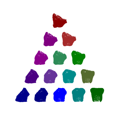
(d) ME (linear): $100$ atoms.

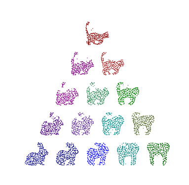
(e) ME (Gaussian): $100$ atoms.

(f) L-BW: $100$ atoms.

Figure 8: Visualization of barycenters for different methods: The coordinates represent the Wasserstein simplex, which consists in all of their Wasserstein barycenters under varying weights $\boldsymbol{\lambda}\in\Delta^{3}$. (top) row corresponds to $k=10$; (bottom) row corresponds to $k=100$.

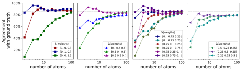
(a) ME (Linear)

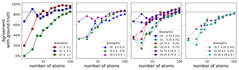
(b) ME (Gaussian)

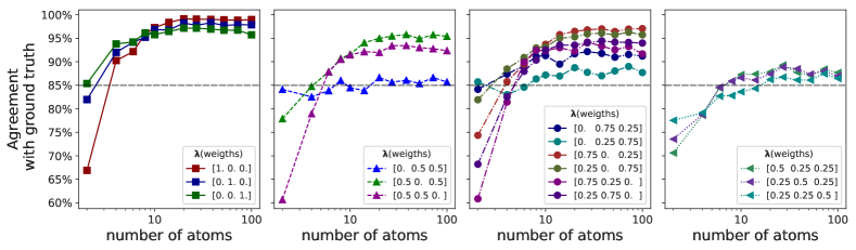
(c) L-BW

Figure 9: Support recovery on simulated data: Evaluation of the performance varying the number $k$ of atoms, for barycenters obtained with different weights $\boldsymbol{\lambda}\in\Delta^{3}$. Coordinates in the Wasserstein simplex represent shapes: cat ($\boldsymbol{\lambda}=[1,0,0]$), rabbit ($\boldsymbol{\lambda}=[0,1,0]$), and tooth ($\boldsymbol{\lambda}=[0,0,1]$). The horizontal dashed line denotes $85\%$ of the agreement.

7.2 Statistical-parity fairness experiment

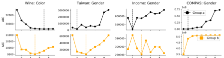
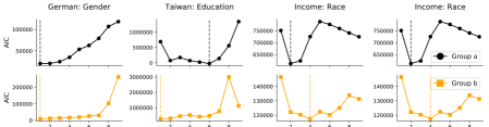
Figure 12: Setting the number of components: The AIC as a function the number of Gaussian components for all datasets and sensitive conditions. For most of the datasets, the optimal number of components is different for each sensitive group.

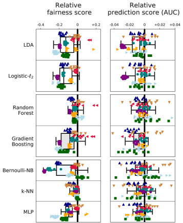
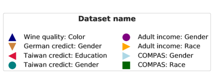
Figure 13: Impact of mixing distributions with L-BW on performance of various conventional classifiers: The performance of classifiers after mixing groups relative to mean scores of the raw classifier. The fairness score, the lower, the better ($<0$). The AUC, the higher, the better ($>0$). Mixing groups improves the fairness for most methods while preserving the predictive accuracy.

Fig.13 shows the impact of mixing groups by L-BW in various conventional classifiers: Logistic regression ($\ell_{2}$ penalty), Naive Bayes (Bernoulli), k-Nearest Neighbors (k-NN), Linear Discriminant Analysis (LDA), Gradient Boosting Trees ($100$ trees), Random Forest ($100$ trees), and Multi Layer Perceptron (MLP, $100$ hidden units and ReLu as activation function). The fairness score (DP-$\gamma$) of K-NN and Random-Forest does not display any improvement, whereas the other classifiers present significant results ($\text{p}_{\text{value}}<10^{-8}$, paired Wilcoxon rank test). L-BW reduces the predictive performance of Gradient Boosting Trees and Linear Discriminant Analysis. Contrary to other classifiers, where the difference to the raw classifier is not significant.

References

- Arjovsky et al. [2017] M. Arjovsky, S. Chintala, and L. Bottou. Wasserstein gan. arXiv preprint arXiv:1701.07875, 2017.
- Bach and Jordan [2005] F. R. Bach and M. I. Jordan. Predictive low-rank decomposition for kernel methods. In ICML. ACM, 2005.
- Bhatia et al. [2018] R. Bhatia, T. Jain, and Y. Lim. On the bures–wasserstein distance between positive definite matrices. Expositiones Mathematicae, 2018.
- Blake [1998] C. Blake. Uci repository of machine learning databases. http://www. ics. uci. edu/~ mlearn/MLRepository. html, 1998.
- Bonneel et al. [2011] N. Bonneel, M. Van De Panne, S. Paris, and W. Heidrich. Displacement interpolation using lagrangian mass transport. In ACM Transactions on Graphics (TOG), volume 30. ACM, 2011.
- Burkard et al. [2009] R. E. Burkard, M. Dell’Amico, and S. Martello. Assignment problems. Springer, 2009.
- Courty et al. [2017] N. Courty, R. Flamary, D. Tuia, and A. Rakotomamonjy. Optimal transport for domain adaptation. IEEE TPAMI, 39, 2017.
- Cuturi [2013] M. Cuturi. Sinkhorn distances: Lightspeed computation of optimal transport. In NeurIPS, 2013.
- Cuturi and Doucet [2014] M. Cuturi and A. Doucet. Fast computation of wasserstein barycenters. In ICML, 2014.
- del Barrio et al. [2018] E. del Barrio, F. Gamboa, P. Gordaliza, and J.-M. Loubes. Obtaining fairness using optimal transport theory. arXiv preprint arXiv:1806.03195, 2018.
- Flamary and Courty [2017] R. Flamary and N. Courty. Pot python optimal transport library, 2017. URL https://github.com/rflamary/POT.
- Flamary et al. [2018] R. Flamary, M. Cuturi, N. Courty, and A. Rakotomamonjy. Wasserstein discriminant analysis. Machine Learning, 107, 2018.
- Friedman et al. [2001] J. Friedman, T. Hastie, and R. Tibshirani. The elements of statistical learning, volume 1. Springer series in statistics New York, 2001.
- Genevay et al. [2018] A. Genevay, G. Peyre, and M. Cuturi. Learning generative models with sinkhorn divergences. In AISTATS, 2018.
- Givens et al. [1984] C. R. Givens, R. M. Shortt, et al. A class of wasserstein metrics for probability distributions. The Michigan Mathematical Journal, 31, 1984.
- Jones et al. [2014] E. Jones, T. Oliphant, and P. Peterson. SciPy: Open source scientific tools for Python. 2014.
- Larson et al. [2016] J. Larson, S. Mattu, L. Kirchner, and J. Angwin. How we analyzed the compas recidivism algorithm. ProPublica (5 2016), 9, 2016.
- Masarotto et al. [2018] V. Masarotto, V. M. Panaretos, and Y. Zemel. Procrustes metrics on covariance operators and optimal transportation of gaussian processes. Sankhya A, 2018.
- Munkres [1957] J. Munkres. Algorithms for the assignment and transportation problems. Journal of the society for industrial and applied mathematics, 5, 1957.
- Olfat and Aswani [2018] M. Olfat and A. Aswani. Spectral algorithms for computing fair support vector machines. In AISTATS, 2018.
- Otsu [1979] N. Otsu. A threshold selection method from gray-level histograms. IEEE transactions on systems, man, and cybernetics, 9, 1979.
- Pedregosa et al. [2011] F. Pedregosa, G. Varoquaux, A. Gramfort, V. Michel, B. Thirion, O. Grisel, M. Blondel, P. Prettenhofer, R. Weiss, V. Dubourg, J. Vanderplas, A. Passos, D. Cournapeau, M. Brucher, M. Perrot, and E. Duchesnay. Scikit-learn: Machine learning in Python. JMLR, 12, 2011.
- Perrot et al. [2016] M. Perrot, N. Courty, R. Flamary, and A. Habrard. Mapping estimation for discrete optimal transport. In NeurIPS, 2016.
- Peyré et al. [2019] G. Peyré, M. Cuturi, et al. Computational optimal transport. Foundations and Trends® in Machine Learning, 11, 2019.
- Rabin et al. [2011] J. Rabin, G. Peyré, J. Delon, and M. Bernot. Wasserstein barycenter and its application to texture mixing. In International Conference on Scale Space and Variational Methods in Computer Vision. Springer, 2011.
- Schmitz et al. [2018] M. A. Schmitz, M. Heitz, N. Bonneel, F. Ngole, D. Coeurjolly, M. Cuturi, G. Peyré, and J.-L. Starck. Wasserstein dictionary learning: Optimal transport-based unsupervised nonlinear dictionary learning. SIAM Journal on Imaging Sciences, 11, 2018.
- Solomon et al. [2015] J. Solomon, F. De Goes, G. Peyré, M. Cuturi, A. Butscher, A. Nguyen, T. Du, and L. Guibas. Convolutional wasserstein distances: Efficient optimal transportation on geometric domains. ACM Transactions on Graphics (TOG), 34, 2015.
- Takatsu et al. [2011] A. Takatsu et al. Wasserstein geometry of gaussian measures. Osaka Journal of Mathematics, 48, 2011.
- Tolstikhin et al. [2017] I. Tolstikhin, O. Bousquet, S. Gelly, and B. Schoelkopf. Wasserstein auto-encoders. arXiv preprint arXiv:1711.01558, 2017.
- Villani [2008] C. Villani. Optimal transport: old and new, volume 338. Springer Science & Business Media, 2008.
- [31] J. Ye, P. Wu, J. Z. Wang, and J. Li. Fast discrete distribution clustering using wasserstein barycenter with sparse support. IEEE Transactions on Signal Processing, 65.
- Zafar et al. [2017] M. B. Zafar, I. Valera, M. G. Rogriguez, and K. P. Gummadi. Fairness constraints: Mechanisms for fair classification. In AISTATS, 2017.
- Zaharia et al. [2016] M. Zaharia, R. S. Xin, P. Wendell, T. Das, M. Armbrust, A. Dave, X. Meng, J. Rosen, S. Venkataraman, M. J. Franklin, et al. Apache spark: a unified engine for big data processing. Communications of the ACM, 59, 2016.