Scale-invariant estimates and vorticity alignment for Navier-Stokes in the half-space with no-slip boundary conditions

Abstract This paper is concerned with geometric regularity criteria for the Navier-Stokes equations in $\mathbb{R}^{3}_{+}\times(0,T)$ with no-slip boundary condition, with the assumption that the solution satisfies the ‘ODE blow-up rate’ Type I condition. More precisely, we prove that if the vorticity direction is uniformly continuous on subsets of

$$\bigcup_{t\in(T-1,T)}\big{(}B(0,R)\cap\mathbb{R}^{3}_{+}\big{)}\times{\{t\}},\,\,\,\,\,\,R=O(\sqrt{T-t})$$

where the vorticity has large magnitude, then $(0,T)$ is a regular point. This result is inspired by and improves the regularity criteria given by Giga, Hsu and Maekawa in [20]. We also obtain new local versions for suitable weak solutions near the flat boundary. Our method hinges on new scaled Morrey estimates, blow-up and compactness arguments and ‘persistence of singularites’ on the flat boundary. The scaled Morrey estimates seem to be of independent interest.

Keywords  Navier-Stokes equations, half-space, boundary regularity, geometric regularity criteria, vorticity alignment, Type I blow-up, Morrey spaces, persistence of singularities.

Mathematics Subject Classification (2010)  35A99, 35B44, 35B65, 35D30, 35Q30, 76D05

1. Introduction

This paper concerns the Navier-Stokes system in the half-space $\mathbb{R}^{3}_{+}:=\{(x^{\prime},x_{3})\in\mathbb{R}^{3},\,\,\,\,x_{3}>0\}$ with no-slip boundary condition:

(1) $$\partial_{t}u-\Delta u+u\cdot\nabla u+\nabla p=0,\,\,\,\,u(x,0)=u_{0}\,\,\,\,\,\nabla\cdot u=0,\,\,\,u|_{\partial\mathbb{R}^{3}_{+}}=0,\,\,\,\,x\in\mathbb{R}^{3}_{+}\,\,\,\,\,t>0.$$

For the simplest case of the fluid occupying the whole-space $\mathbb{R}^{3}$, it is a Millennium prize problem [18] as to whether or not solutions to the Navier-Stokes equations, with Schwartz class divergence-free initial data, remain smooth for all times.

In [11], Constantin and Fefferman provided a geometric regularity criteria for the vorticity $\omega=\nabla\times u$ of solutions on the whole-space, which remarkably does not depend on scale-invariant quantities. Specifically, they showed that if

(2) $$|\sin(\angle(\omega(x+y,t),\omega(x,t))|\leq C|y|\\ \,\,\,\,\textrm{for}\,\,\,\,(x,t)\in\Omega_{d}:=\{(y,s)\in\mathbb{R}^{3}\times(0,T):|\Omega(y,s)|>d\}$$

then $u$ is smooth on $\mathbb{R}^{3}\times(0,T]$. Their proof uses energy estimates for the vorticity equation

(3) $$\partial_{t}\omega-\Delta\omega+u\cdot\nabla\omega-\omega\cdot\nabla u=0$$

to get

(4) $$\|\omega(\cdot,t)\|_{L_{2}(\mathbb{R}^{3})}^{2}+2\int\limits_{0}^{t}\int\limits_{\mathbb{R}^{3}}|\nabla w|^{2}dxdt\leq 2\int\limits_{0}^{t}\int\limits_{\mathbb{R}^{3}}(\omega\cdot\nabla u)\cdot\omega dxdt$$

Then Constantin and Fefferman proceed with a careful analysis of the stretching term

$$\int\limits_{0}^{t}\int\limits_{\mathbb{R}^{3}}(\omega\cdot\nabla u)\cdot\omega dxdt.$$

In particular, the Biot-Savart law, integration by parts and linear algebra identities are used to show that the most singular contribution of the stretching term can be controlled by

(5) $$\int\limits_{0}^{t}\iint\limits_{\Omega_{d}\times\Omega_{d}}\frac{|\omega(x,s)|^{2}|\omega(y,s)||\sin(\angle{(\omega(y,s),\omega(x,s)})|}{|x-y|^{3}}dydxds.$$

Crucially (2) depletes the singularity in the integral of this stretching term. For certain extensions of this geometric regularity criterion, we refer (non-exhaustively) to [14, 25, 51, 26, 24, 22, 32].

For the case of the Navier-Stokes equations in $\mathbb{R}^{3}_{+}$ with no-slip boundary conditions (1), vorticity is generated at the boundary. Specifically, $\omega$ has a non-zero trace on $\partial\mathbb{R}^{3}_{+}$. This provides a block to applying energy methods to the vorticity equation (3). Consequently, the following remains open

• (Q): For finite energy solutions of the Navier-Stokes equations in $\mathbb{R}^{3}_{+}\times(0,T)$, with no-slip boundary condition and divergence-free initial data $u_{0}\in C^{\infty}_{0}(\mathbb{R}^{3}_{+})$, does (2) imply that $u$ is smooth on $\mathbb{R}^{3}_{+}\times(0,T]$?

Note that with perfect slip boundary conditions

(6) $$u_{3}=\partial_{3}u_{2}=\partial_{2}u_{1}\,\,\,\,\,\textrm{on}\,\,\,\,\,\,\partial{\mathbb{R}}^{3}_{+},\qquad u=(u_{1},u_{2},u_{3}),$$

vorticity is not created at the boundary and the geometric regularity condition is known to hold [13]. The issue of vorticity creation at the boundary has meant that certain other situations that are understood for the Navier-Stokes equations in the whole-space $\mathbb{R}^{3}$, remain open for the case of the fluid occupying the half-space with no-slip boundary condition. Two such examples are:

1. Existence of backward self-similar solutions

   $$u(x,t)=\frac{1}{\sqrt{T-t}}U\Big{(}\frac{x}{\sqrt{T-t}}\Big{)},\,\,\,\,(x,t)\in\mathbb{R}^{3}_{+}\times(0,T)$$

   with finite local energy and no-slip boundary condition. For the whole-space such solutions were shown not to exist in [50].

2. Smoothness of solutions to the Navier-Stokes equations in $\mathbb{R}^{3}_{+}\times(0,\infty)$ with no-slip boundary condition that are axisymmetric without swirl. Such solutions have the following form in cylindrical coordinates

   $$u(r,z,t)=u_{r}(r,z)\vec{e}_{r}+u_{z}(r,z)\vec{e}_{z},$$

   where $\vec{e}_{r}=(\cos(\theta),\sin(\theta),0)$, $\theta\in(-\pi,\pi)$ and $\vec{e}_{z}=(0,0,1).$ For the whole-space, such solutions were shown to be smooth in [31].

To the best of our knowledge, the only vorticity alignment regularity criteria known for the Navier-Stokes equations in $\mathbb{R}^{3}_{+}\times(0,T)$ (with no-slip boundary condition), was proven by Giga, Hsu and Maekawa in [20] for mild solutions under the additional assumption that $u$ satisfies the Type I condition (8) (see below in Theorem 1). In particular, in [20] it was shown that if $\eta:[0,\infty)\rightarrow\mathbb{R}$ is a nondecreasing continuous function with $\eta(0)=0$ , $\xi=\frac{\omega}{|\omega|}$ and $\Omega_{d}:=\{(x,t)\in\mathbb{R}^{3}_{+}\times(0,T):|\omega(x,t)|>d\}$ then the following holds true. Namely, the assumption

(7) $$|\xi(x,t)-\xi(y,t)|\leq\eta(|x-y|)\,\,\,\,\,\textrm{for}\,\,\textrm{all}\,\,(x,t),(y,t)\in\Omega_{d}$$

implies that $u$ is bounded up to $t=T$.

The main goal of our paper is to prove a vorticity alignment regularity criteria, for the Navier-Stokes equations in $\mathbb{R}^{3}_{+}\times(0,T)$ with no-slip boundary condition, that improves upon the result in [20]. In what follows, we say that $(x_{0},T)$ is a ‘regular point’ of $u$ if there exists $r>0$ such that $u\in L^{\infty}((B(x_{0},r)\cap\mathbb{R}^{3}_{+})\times(T-r^{2},T))$. Any point that is not regular is defined to be a ‘singular point’. Let us state our main theorem below.

Theorem 1.

Suppose $u$ is a mild solution to the Navier-Stokes equations in $\mathbb{R}^{3}_{+}\times(0,T)$, $(T>1)$, with no-slip boundary condition $u|_{\partial\mathbb{R}^{3}_{+}}=0$ and with divergence-free initial data $u_{0}\in C^{\infty}_{0}(\mathbb{R}^{3}_{+}).$ Furthermore, suppose that for $(x,t)\in\mathbb{R}^{3}_{+}\times(0,T)$:

(8) $$|u(x,t)|\leq\frac{M}{\sqrt{T-t}}.$$

Let $t^{(n)}\uparrow T$, $x_{0}\in\mathbb{R}^{3}_{+}\cup\partial\mathbb{R}^{3}_{+}$, $d>0$ and $\delta>0$. Define $\omega=\nabla\times u$, $\xi:=\frac{\omega}{|\omega|}$, the set of high vorticity,

$$\Omega_{d}:=\{(x,t)\in\mathbb{R}^{3}_{+}\times(0,T):|\omega(x,t)|>d\},$$

the cone

$$\mathcal{C}_{\delta,x_{0}}:=\bigcup_{t\in(T-1,T)}\{x\in\mathbb{R}^{3}_{+}:|x-x_{0}|<\delta\sqrt{T-t_{0}}\}$$

and the time-sliced cone

$$\mathcal{C}_{t^{(n)},\delta,x_{0}}:=\bigcup_{n}\{(x,t^{(n)}):x\in\mathbb{R}^{3}_{+}\,\,\,\textrm{and}\,\,\,|x-x_{0}|<\delta\sqrt{T-t^{(n)}}\}.$$

Let $\eta:\mathbb{R}\rightarrow\mathbb{R}$ be a continuous function with $\eta(0)=0$.
Under the above assumptions, there exists $\delta(M,u_{0})>0$ such that the following holds true: on the one hand

(9) $$\sup_{(x,t)\in\mathcal{C}_{t^{(n)},\delta,x_{0}}}|\omega(x,t)|<\infty\Rightarrow\,\,\,\,\,\,(x_{0},T)\quad\mbox{is a regular point of}\quad u,$$

and on the other hand

(CA) $$|\xi(x,t)-\xi(y,t)|\leq\eta(|x -y|)\,\,\,\,\,\,\,\,\,\,\,\,\,\,\,\textrm{in}\,\,\,\,\,\Omega_{d}\cap\mathcal{C}_{\delta,x_{0}}$$

$$\Downarrow$$

$$(x_{0},T)\quad\mbox{is a}\ \mbox{regular point of}\quad u.$$

The condition (CA) is dubbed the ‘continuous alignment condition’.

Remark 1.

In this paper we also obtain local variations of Theorem 1. To the best of the authors’ knowledge those are the first local results regarding regularity under the vorticity alignment condition, for a Navier-Stokes solution having no-slip on the flat part of the boundary. Previously all localisations were known for only interior cases [26, 24, 22]. For precise statements of our local results, we refer the reader to Section 6 ‘Geometric regularity criteria near a flat boundary: local setting’.

Remark 2.

When $x_{0}$ is a regular point of $u$ belonging to the interior of the half-space, it can be seen that $u$ has Hölder continuous spatial derivatives near $x_{0}$ and the converse statement to Theorem 1 is true, i.e. the vorticity alignment condition (CA) holds. It is not clear to the authors whether or not that remains to be the case when $x_{0}$ lies on $\partial\mathbb{R}^{3}_{+}$. The difficulty is that there are examples in [27] and [42], for a Navier-Stokes solution in the local setting with no-slip boundary condition on the flat part of the boundary, that demonstrate that boundedness of $u$ near the flat boundary does not imply boundedness of $\nabla u$. It is interesting to note that these examples do not provide a counterexample to the converse statement of Theorem 1. In fact in [42] the construction is based upon a monotone shear flow, whose vorticity direction is constant.

1.1. Comparison of Theorem 1 to previous literature and novelty of our results

In [20] progress was made at establishing the geometric regularity criteria for the vorticity when the fluid occupies the half-space $\mathbb{R}^{3}_{+}$ with no-slip boundary condition, with the additional assumption that the solution satisfies Type I bounds. As we mention above, the geometric regularity criterion remains in general an outstanding open problem when the fluid occupies the half-space $\mathbb{R}^{3}_{+}$ with no-slip boundary condition. Let us now state the result first proven in [20].

Theorem ([20, Theorem 1.3]).

Suppose $u$ is a mild solution to the Navier-Stokes equations in $\mathbb{R}^{3}_{+}\times(0,T)$ with boundary condition $u|_{\partial\mathbb{R}^{3}_{+}}=0$ and with divergence-free initial data $u_{0}\in C^{\infty}_{0}(\mathbb{R}^{3}_{+})$. Let $d$ be a positive number and let $\eta$ be a nondecreasing continuous function on $[0,\infty)$ satisfying $\eta(0)=0$. Assume that $\eta$ is a modulus of continuity in the $x$ variables for the vorticity direction $\xi=\omega/|\omega|$, in the sense that

(10) $$|\xi(t,x)-\xi(t,y)|\leq\eta(|x-y|)\,\,\,\,\,\,\textrm{for}\,\,\textrm{all}\,\,\,\,\,(x,t),(y,t)\in\Omega_{d},$$

where $\Omega_{d}$ is defined in Theorem 1. Then $u$ is bounded up to $t=T$.

The proof in [20] relies on two steps:

1. Using the assumption (10) and a choice of suitable rescalings for the equation (blow-up procedure) to reduce to a non zero two-dimensional nontrivial bounded limit solution with positive vorticity, which is defined on either the whole-space or the half-space. This limiting solution to the Navier-Stokes equations belongs to one of two special classes called ‘whole-space mild bounded ancient solutions’ or ‘half-space mild bounded ancient solutions’. We refer the reader to subsection 1.3 for the definitions and discussion of these objects.

2. Obtaining a contradiction by showing the limit function must be zero. This is done in [22] and [20] by proving a Liouville theorem for two-dimensional whole-space and half-space mild bounded ancient solutions having positive vorticity and satisfying the bound

   $$\sup_{t<0}(-t)^{\frac{1}{2}}\|u(\cdot,t)\|_{L_{\infty}}<\infty.$$

The rescaling used in the first step is very specific. Let $t^{(k)}\uparrow T$, $y^{(k)}$ and $R_{k}\downarrow 0$ be selected such that

(11) $$\frac{1}{R^{(k)}}-1\leq|u(y^{(k)},t^{(k)})|\leq\sup_{0\leq s\leq t^{(k)}}\|u(\cdot,s)\|_{L_{\infty}(\mathbb{R}^{3})}:=\frac{1}{R^{(k)}}.$$

Then $u^{(k)}(y,t)=R^{(k)}u\big{(}R^{(k)}(y+y^{(k)}),(R^{(k)})^{2}(t+t^{(k)})\big{)}$ produces either a whole-space or half-space mild bounded ancient solution $u^{(\infty)}$ in the limit. By [8, Theorem 1.3], $u^{(\infty)}$ is smooth in space-time. To reach a contradiction, it is hence necessary to prove a strong fact about the limit, namely that the mild bounded ancient solution is zero. This is the purpose of the second step. For the case of the half-space, this step is nontrivial and involves a delicate analysis of the vorticity equation and its boundary condition.

The purpose of our work is to pave the way for a new method to prove regularity under the vorticity alignment and Type I condition. This new approach allows more flexibility in the rescaling procedure. To reach a contradiction, we do not need to show that the blow-up profile $u^{(\infty)}$ is zero. Instead it suffices to prove that it is bounded at a specific point, which is much easier. The vorticity alignment condition serves the purpose of showing that $u^{(\infty)}$ is close to a two-dimensional flow in certain weak topologies. This is sufficient to infer that $u^{(\infty)}$ is bounded at the desired point.

Our strategy allows to prove regularity under the Type I condition, assuming vorticity alignment on concentrating sets, as in Theorem 1. It also makes it possible to achieve local versions of the result of Giga, Hsu and Maekawa [20, Theorem 1.3], and of our main result, Theorem 1. For such statements, we refer to Theorem 4 and Remark 17 in Section 6. As far as we know, the global or local statements with vorticity alignment on concentrating sets are new even for the case of the whole-space $\mathbb{R}^{3}$.

The keystone in our scheme is the stability of singularities for the Navier-Stokes equations. Stability of singularities and compactness arguments were also used in [1, Theorem 4.1 and Remark 4.2] and [2, Theorem 3.1 and Lemma 3.3] to prove some regularity criteria. The following lemma is a crucial tool. It is taken from the first author’s Thesis [6, Proposition 5.5]; see also [2, Proposition A.5] and [37, Proposition 5.21] for subsequent generalisations. The stability of singular points was first proven in the interior case by Rusin and Šverák [38]. In the Lemma below and throughout this paper, we define $B^{+}(r):=B(r)\cap\mathbb{R}^{3}_{+}$ and $Q^{+}(1):=B^{+}(1)\times(-1,0)$. We refer the reader to subsection 1.5, for the definition of suitable weak solutions in $Q^{+}(1)$.

Lemma 3.

Suppose $(u^{(k)},p^{(k)})$ are suitable weak solutions to the Navier-Stokes equations in $Q^{+}(1)$. Suppose that there exists a finite $M>0$ such that

(12) $$\sup_{k}\Big{(}\|u^{(k)}\|_{L_{2}^{t}L_{\infty}^{x}(Q^{+}(1))}+\|\nabla u^{(k)}\|_{L_{2}(Q^{+}(1))}+\|p^{(k)}\|_{L_{\frac{3}{2}}(Q^{+}(1))}\Big{)}=M<\infty.$$

Furthermore assume that

(13) $$\lim_{k\rightarrow\infty}\|u^{(k)}-u^{(\infty)}\|_{L_{3}(Q^{+}(1))}=0,$$

(14) $$p^{(k)}\rightharpoonup p^{(\infty)}\,\,\textrm{in}\,\,L_{\frac{3}{2}}(Q^{+}(1)),$$

$$(0,0)\quad\mbox{is a singular point of}\quad u^{(k)}\quad\mbox{for all}\quad k=1,2\ldots$$

Then the above assumptions imply that $(u^{(\infty)},p^{(\infty)})$ is a suitable weak solution to the Navier-Stokes equations in $Q^{+}(1)$ with $(0,0)$ being a singular point of $u^{(\infty)}$.

To show more precisely how our proof of Theorem 1 works, let us assume for contradiction that $u$ is singular at the space-time point $(0,T)$. Let $R_{k}\downarrow 0$ be any sequence. We rescale in the following way

(15) $$u^{(k)}(y,s):=R_{k}u(R_{k}y,T+R_{k}^{2}s)\,\,\,\,\textrm{and}\,\,p^{(k)}(y,s):=R_{k}^{2}p(R_{k}y,T+R_{k}^{2}s),$$

for all $y\in\mathbb{R}^{3}_{+}$ and $s\in(-T/R_{k}^{2},0)$. We show that the Type I condition (8) implies the boundedness of the following scale-invariant quantities

(16) $$\sup_{0<r<1}\Bigg{\{}\frac{1}{r}\sup_{T-r^{2}<t<T}\int\limits_{B^{+}(r)}|u(x,t)|^{2}dx+\frac{1}{r}\int\limits_{T-r^{2}}^{T}\int\limits_{B^{+}(r)}|\nabla u|^{2}dxdt\\ +\frac{1}{r^{2}}\int\limits_{T-r^{2}}^{T}\int\limits_{B^{+}(r)}|p-(p)_{B^{+}(r)}|^{\frac{3}{2}}dxdt\Bigg{\}}<\infty.$$

Hence (12) holds for $(u^{(k)},p^{(k)})$ and we can apply Lemma 3. While this implication is well-known in the whole-space, it is a main technical block in the half-space. One of our main achievements in this paper is to overcome this technical block. We explain this in more details in the paragraph 1.2 below.

Applying Lemma 3 gives us the following. Namely the blow-up profile $u^{(\infty)}$ (obtained from $u^{(k)}$ in the limit) is an ancient mild solution, which has a singularity at $(0,0)$, satisfies the Type I assumption and has bounded scaled energy. Moreover, the continuous alignment condition for the vorticity implies that the vorticity direction of $u^{(\infty)}$ is constant in a large ball. We can then reach a contradiction by the following proposition for $\bar{u}=u^{(\infty)}$, proved in Section 4.

Proposition 4.

Suppose that $(\bar{u},\bar{p})$ is a mild solution to the Navier-Stokes equations on $\mathbb{R}^{3}_{+}\times(-\infty,0)$ with $\bar{u}|_{\partial\mathbb{R}^{3}_{+}}=0.$ Let $\bar{\omega}:=\nabla\times\bar{u}$ and suppose $(\bar{u},\bar{p})$ is a suitable weak solution to the Navier-Stokes equations on $\mathbb{R}^{3}_{+}\times(-\infty,0)$. Furthermore suppose that

(17) $$|\bar{u}(x,t)|\leq\frac{M}{\sqrt{-t}}$$

and

(18) $$\sup_{0<r<\infty}\Bigg{\{}\frac{1}{r}\sup_{-r^{2}<t<0}\int\limits_{B^{+}(r)}|\bar{u}(x,t)|^{2}dx+\frac{1}{r}\int\limits_{Q^{+}(r)}|\nabla\bar{u}|^{2}dxdt\\ +\frac{1}{r^{2}}\int\limits_{Q^{+}(r)}|\bar{p}-(\bar{p}(\cdot,t))_{B^{+}(r)}|^{\frac{3}{2}}dxdt\Bigg{\}}\leq M^{\prime}.$$

Under the above assumptions the following holds true. For all $M$ and $M^{\prime}>0$, there exists $\gamma(M,M^{\prime})>0$ such that if

(19) $$\bar{\omega}(x,-t_{0})\cdot\vec{e}_{i}=0\,\,\,\,\,\textrm{in}\,\,\,\,B^{+}(\gamma(M,M^{\prime})\sqrt{t_{0}})\,\,\mbox{for}\ i=2,3\,\,\,\,\mbox{and}\,\,\,\mbox{some}\,\,\,\,t_{0}\in(0,\infty)$$

then $(x,t)=(0,0)$ is a regular point for $\bar{u}$.

The main flexibility of our method lies in the fact that we can use any sequence $R^{(k)}\downarrow 0$ in the rescaling procedure. Therefore, we can tune the sequence to our needs. In the case of the whole-space, we can take advantage of this versatility on time slices of the cone (Theorem 3 in Section 5) and not the whole-cone as in Theorem 1.

Remark 5 (alternative argument suggested by Seregin).

Gregory Seregin suggested to the authors that bounded scaled energy quantities for $u$ such as (16) could be used to reprove the theorem of Giga, Hsu and Maekawa [20, Theorem 1.3] in the following way. His idea is to show that the existence of a singular solution satisfying (10) and (16) implies the existence of either a non-trivial two-dimensional whole-space or half-space mild bounded ancient solution $\bar{u}$ in $\Omega\times(-\infty,0)$ ($\Omega=\mathbb{R}^{3}$ or $\mathbb{R}^{3}_{+}$) satisfying

(20) $$\sup_{0<r<\infty}\sup_{-r^{2}<t<0}\frac{1}{r}\int\limits_{B(r)\cap\Omega}|\bar{u}(x_{1},x_{3},t)|^{2}dx_{1}dx_{2}dx_{3}<\infty.$$

This then implies that either $\bar{u}\in L^{\infty}(-\infty,0;L^{2}(\mathbb{R}^{2}))$ or $L^{\infty}(-\infty,0;L^{2}(\mathbb{R}^{2}_{+}))$. Such a $\bar{u}$ then must be zero by applying a Liouville theorem proven in [28] (for the whole-space case) and a Liouville theorem by Seregin in [39] (for the half-space case). This contradiction then implies regularity under the assumptions (10) and (16).

Our approach avoids resorting to a Liouville theorem. Under the ‘ODE blow-up rate’ assumption (8), we gain additional information about the blow-up profile. Namely,

$$|u^{(\infty)}(x,t)|\leq\frac{M}{\sqrt{-t}}.$$

This plays an important role in our proof. Specifically, it ensures that for $t_{0}>0$, $u^{(\infty)}$ is the unique strong solution to the Navier-Stokes equations on $\mathbb{R}^{3}_{+}\times(-t_{0},0)$ with initial data $u^{(\infty)}(\cdot,-t_{0})$. It is not known if such considerations apply to the case when $u^{(\infty)}$ satisfies (20).

We now explain how we get over the main technical block in this argument, namely to prove that the Type I assumption (8) implies the boundedness of scaled energies (16).

1.2. Scale-invariant estimates

Let $\Omega$ be a domain in $\mathbb{R}^{3}$. We define the following scale-invariant quantities, which will be used throughout our work: for $x\in\bar{\Omega}$, $r\in(0,\infty)$

(21) $$A(u,r;x,t):=\ \sup_{t-r^{2}<s<t}\frac{1}{r}\int\limits_{B(x,r)\cap\Omega}|u(y,s)|^{2}dy,$$

(22) $$E(u,r;x,t):=\ \frac{1}{r}\int\limits_{t-r^{2}}^{t}\int\limits_{B(x,r)\cap\Omega}|\nabla u|^{2}dyds,$$

(23) $$D_{\frac{3}{2}}(p,r;x,t):=\ \frac{1}{r^{2}}\int\limits_{t-r^{2}}^{t}\int\limits_{B(x,r)\cap\Omega}|p-(p(\cdot,s))_{B(x,r)\cap\Omega}|^{\frac{3}{2}}dyds.$$

Here and throughout this paper,

$$(f)_{\Omega}:=\frac{1}{|\Omega|}\int\limits_{\Omega}f(y)dy.$$

Below, we will often take $(x,t)=(0,0)$, as well as $\Omega=B^{+}(1)$, $B(1)$, $\mathbb{R}^{3}_{+}$, or $\mathbb{R}^{3}$. In this case, we have the following lighter notation:

(24) $$A(u,r):=A(u,r;0,0),\quad E(u,r):=E(u,r;0,0),\quad D_{\frac{3}{2}}(p,r;x,t):=D_{\frac{3}{2}}(p,r;0,0).$$

Away from boundaries it is known that for a suitable weak solution $(u,p)$ of the Navier-Stokes equations in $Q(1)$, the Type I condition

(25) $$|u(x,t)|\leq\frac{M}{\sqrt{-t}}\,\,\,\,\,\textrm{in}\,\,\,\,Q(1)$$

implies

$$\sup_{0<r<1}\big{\{}A(u,r)+E(u,r)+D_{\frac{3}{2}}(p,r)\big{\}}<\infty.$$

This was established by Seregin and Zajaczkowski in [48]; see also Seregin and Šverák [44] (statement and proof) and [3, Lemma 2.5] (statement only). We show that this implication is also true up to a flat boundary. The following theorem is one of our main contributions in this paper, and the key technical tool to prove Theorem 1 as well as its local versions.

Theorem 2.

Suppose that $(u,p)$ is a suitable weak solution of the Navier-Stokes equations in $Q^{+}(1)$ and satisfies the Type I bound

(26) $$|u(x,t)|\leq\frac{M}{\sqrt{-t}}\,\,\,\,\,\textrm{in}\,\,\,\,Q^{+}(1)$$

Then one infers that

(27) $$\sup_{0<r<1}\big{\{}E(u,r)+A(u,r)+D_{\frac{3}{2}}(p,r)\big{\}}\leq M^{\prime}\big{(}M,A(u,1),E(u,1),D_{\frac{3}{2}}(p,1)\big{)}.$$

Let us now discuss a generalized notion of ‘Type I’ blow-up. Suppose that for $\Omega=\mathbb{R}^{3}$ or $\mathbb{R}^{3}_{+}$ there is a suitable weak solution $u$ that loses smoothness at $T$. We then call the singular point $(x_{0},T)\in\bar{\Omega}\times\{T\}$ a Type I singularity if there exists $R>0$ such that

(28) $$\sup_{\begin{subarray}{c}(B(x,r)\cap\Omega)\times(t-r^{2},t)\\ \subset(B(x_{0},R)\cap\Omega)\times(T-R^{2},T)\end{subarray}}\big{(}A(u,r;x,t)+E(u,r;x,t)+D_{\frac{3}{2}}(p,r;x,t)\big{)}<\infty.$$

For the case of a suitable solution $u$ defined on the whole-space, it is discussed in [3] that the definition of Type I singularities given by (28) is very natural and includes most other popular notions of ‘Type I’ used in the literature. For the case of a suitable solution $u:\mathbb{R}^{3}_{+}\times(0,\infty)\rightarrow\mathbb{R}^{3}$ in the half-space with no-slip boundary condition, it was shown in [35] and [40] that the definition of Type I singularity (28) is implied by

$$|u(x,t)|\leq\frac{M}{|x|}.$$

However, it was previously not understood if, for solutions in the half-space with no-slip boundary conditions, (28) was consistent with the ‘ODE blow-up rate’ notion of Type I singularities (25) and (26) commonly found in the literature (see for instance [21]). Theorem 2 fills this gap and demonstrates that, after all, (28) is a reasonable notion of Type I singularity for suitable solutions in the half-space with no-slip boundary condition.

The importance of Theorem 2 lies in the fact that it links the natural notion of Type I blow-up (26) to a workable notion of Type I. Indeed it turns out that the scale-invariant conditions (27) or (28) are exactly what is needed to prove a number of results. This can be seen in particular in three situations:

1. The scale-invariant bound (27) ensures that the rescaled solutions $(u^{(k)},p^{(k)})$ defined by (15) satisfy the uniform bound (12) required for the persistence of singularities.

2. The type I bound (28) ensures that a mild bounded ancient solution originating from $(u,p)$ has some sort of decay at space infinity. This point is discussed in more details in Section 1.3 below.

3. In the paper [7] on concentration phenomena for Type I blow-up solutions of the Navier-Stokes equations, a scale-critical condition such as (28) was used to provide a control in $L_{2,uloc}(\mathbb{R}^{3})$ of a rescaled solution.

In order to prove Theorem 2 a number of innovations are needed. Indeed, the case near a flat boundary is considerably more intricate than the interior case. The proof relies on the local energy inequality (LABEL:localenergyequalityboundary). The main difficulty lies in the estimate for the pressure term

(29) $$I(u,p,r,\Omega):=\int\limits_{-r^{2}}^{0}\int\limits_{B(r)\cap\Omega}pu\cdot\nabla\varphi dxds$$

where $\varphi\in C_{0}^{\infty}(B(r)\times(-r^{2},\infty))$ is a positive test function and $\Omega=B^{+}(1)$, see (LABEL:localenergyequalityboundary).

To highlight the difficulties concerned with the flat boundary, let us first discuss the proof of the simpler interior case of Theorem 2 [48, 44]. For the Navier-Stokes equations in the whole space (with sufficient decay), the Calderón Zygmund theory gives that the pressure $p$ can be estimated directly in terms of $u\otimes u$, which we write in a formal way $p\simeq u\otimes u$. For the interior case of a suitable weak solution in $Q(1)$, this fact implies the decay estimate

(30) $$D_{\frac{3}{2}}(p,\tau r)\leq C\big{(}\tau D_{\frac{3}{2}}(p,r)+\tau^{-2}C(u,r)\big{)},$$

for a given $\tau\in(0,1)$ and all $r\in(0,1]$. Here,

(31) $$C(u,r):=\frac{1}{r^{2}}\int_{Q(r)}|u|^{3}dxds$$

is a scale-invariant quantity. To prove the interior version of Theorem 2, it then suffices to bound the right hand side of (31). The game to play is to combine energy type quantities and the Type I bound (25) to obtain

(32) $$C(u,r)\lesssim_{M}\ A^{\mu}(u,r)\Biggl{(}\frac{1}{r^{3}}\int\limits_{Q(r)}|u|^{2}dxds+\frac{1}{r}\int\limits_{Q(r)}|\nabla u|^{2}dxds\Biggr{)}^{\theta}$$

$$\Downarrow$$

(33) $$C(u,r)+D_{\frac{3}{2}}(p,\tau r)\lesssim_{M}\ \varepsilon\Biggl{(}\frac{1}{r^{3}}\int\limits_{Q(r)}|u|^{2}dxds+\frac{1}{r}\int\limits_{Q(r)}|\nabla u|^{2}dxds\Biggr{)}$$

$$\qquad\qquad+c(M,\varepsilon,\kappa,\tau)+C\tau D_{\frac{3}{2}}(p,r)$$

with

(34) $$0<\mu,\,\theta,\qquad\kappa:=\mu+\theta<1,\qquad\varepsilon\in(0,1)\quad\mbox{and}\quad c(M,\varepsilon,\kappa,\tau)>0.$$

This estimate is based on interpolation. Figure 1 shows how to obtain it in a clear way. Estimate (32) is critical to get the decay estimate for the energy for $\varepsilon$ and $\tau$ small enough; see [44, estimate (54)].

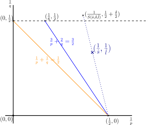
Figure 1. Interpolation for $L_{\hat{l}}^{t}L_{\hat{s}}^{x}(Q^{+}(1))$

In the case of the half-space, on the contrary, we cannot estimate $p$ in terms of $u\otimes u$; in short $p\not\simeq u\otimes u$. This issue is brought up in particular in the work of Koch and Solonnikov [29, Theorem 1.3]. Considering the unsteady Stokes system in the half-space with no-slip boundary conditions, they prove that there are divergence form source terms $\nabla\cdot F$, with $F\in L_{q}^{t,x}$, for which the pressure is not integrable in time. A possible alternative is to use maximal regularity for the Stokes system [23], i.e. $\nabla p\simeq u\cdot\nabla u$. Such an estimate was used for the local boundary regularity theory of the Navier-Stokes theory by Seregin in [45]. It remains a cornerstone for estimating the pressure locally near the boundary. Formally applying the maximal regularity estimate, together with the Poincaré-Sobolev and Hölder inequalities, the estimate of (29) (with $r=1$) turns into

$$\|u\|_{L^{t}_{l}L^{x}_{s}(Q^{+}(1))}\|p-(p)_{B^{+}(1)}(t)\|_{L^{t}_{l^{\prime}}L^{x}_{s^{\prime}}(Q^{+}(1))}\leq\|u\|_{L^{t}_{l}L^{x}_{s}(Q^{+}(1))}\|u\|_{L^{t}_{\hat{l}}L^{x}_{\hat{s}}(Q^{+}(1))}\|\nabla u\|_{L_{2}(Q^{+}(1))}$$

with

(35) $$\frac{1}{l}+\frac{1}{\hat{l}}=\frac{1}{2}\,\,\,\,\textrm{and}\,\,\,\,\,\frac{1}{s}+\frac{1}{\hat{s}}=\frac{5}{6}.$$

The presence of the gradient of $u$ makes this quantity ‘too supercritical’. Using (8) and sharp interpolation arguments (see Lemma 9) give

(36) $$\|u\|_{L^{t}_{l}L^{x}_{s}(Q^{+}(1))}\|u\|_{L^{t}_{\hat{l}}L^{x}_{\hat{s}}(Q^{+}(1))}\lesssim_{M}(A(u,1))^{\lambda}$$

with any $\lambda$ slightly greater than $1-(\frac{1}{l}+\frac{1}{\hat{l}})=\frac{1}{2}$. Thus, any attempt to get an estimate similar to (33) (for $\Omega=B^{+}(1)$) by using maximal regularity estimates for the pressure and the Type I condition (8) will not work. In particular such a strategy will always produce a total power of energy quantities $\kappa\geq 1$, see (34). The analysis of Figure 1 enables to understand the limitation on the exponent $\kappa$. Interpolating the $L_{4}^{t,x}$ norm of $u$ between the energy, i.e. the point $L_{\infty}^{t}L_{2}^{x}$, and the Type I condition, i.e. the region $L_{q}^{t}L_{p}^{x}$, $q<2$, yields a power of the energy too large.

We overcome this difficulty in the half-space thanks to a new estimate on the pressure. The idea is to have an intermediate estimate between $p\simeq u\otimes u$, which is known to be false (see above the comment about [29]), and the maximal regularity estimate $\nabla p\simeq u\cdot\nabla u$, which is too supercritical. Such an estimate was discovered by Chang and Kang [10, Theorem 1.2]. Such ‘fractional’ pressure estimate can be formally written as $\nabla^{\beta}p\simeq\nabla^{\beta}(u\otimes u)$, for $1\geq\beta$ sufficiently close to $1$. We give a new self-contained and straightforward proof of a similar estimate, see Proposition 7. This new proof is based on the pressure formulas for the half-space established in [33, 34]. With the help of the ‘fractional’ pressure estimate, we are able to implement the strategy of [48, 44]. We believe that this is the first instance where the estimate of Chang and Kang [10] (see also Proposition 7 below) is used and is really pivotal.

1.3. Type I singularities, Morrey bounds and ancient solutions

Let us now explain the independent interest of Theorem 2 in clarifying the relationship between Type I singularities (see (28) for a definition) of the Navier-Stokes equations in $\mathbb{R}^{3}_{+}$ with no-slip boundary condition and ‘whole-space mild bounded ancient solutions’ or ‘half-space mild bounded ancient solutions’. These solutions form a special subclass of bounded solutions to Navier-Stokes equations on $\mathbb{R}^{3}\times(-\infty,0)$ and $\mathbb{R}^{3}_{+}\times(-\infty,0)$. For a definition, we refer to [28] for the whole-space and [43] and [8] for the half-space.

Suppose that $u:\mathbb{R}^{3}\times(0,\infty)\rightarrow\mathbb{R}^{3}$ is a solution that first loses smoothness at $T>0$. Let $t^{(k)}\uparrow T$, $y^{(k)}$ and $R_{k}\downarrow 0$ be selected as in (11). In [28], it was shown that in such circumstances, a ‘zooming-in’ procedure of the form

$$u^{(k)}(y,t)=R^{(k)}u\big{(}R^{(k)}(y+y^{(k)}),(R^{(k)})^{2}(t+t^{(k)})\big{)}$$

and

$$p^{(k)}(y,t)=(R^{(k)})^{2}p\big{(}R^{(k)}(y+y^{(k)}),(R^{(k)})^{2}(t+t^{(k)})\big{)}$$

produces a non-zero whole-space mild bounded ancient solution; see also [41] for the localised version of this statement. For the case that $u:\mathbb{R}^{3}_{+}\times(0,\infty)\rightarrow\mathbb{R}^{3}$ is a solution to the Navier-Stokes equations with no-slip boundary condition that first loses smoothness at $T>0$, the ‘zooming in’ procedure produces either non-zero whole-space or non-zero half-space mild bounded ancient solutions; see [43], as well as [2] for the localised statement. In [28] and [43] the following Liouville conjectures were made

(C1):

Any whole-space mild bounded ancient solutions is a constant, see [28].

(C2):

Any half-space mild bounded ancient solution is zero, see [43].

At the moment, these Liouville conjectures are only known to hold in special situations; see [28], [41], [3] for special cases where (C1) holds and see [39] and [20] for two-dimensional cases where (C2) holds.

When one assumes only ‘Type I’ singularities at $T$ in the sense of (28), one gains extra information regarding the whole-space (resp. half-space) mild bounded ancient solutions $u^{(\infty)}$ arising from $u$. In particular, one gets

(37) $$\sup_{(x,t)\in\bar{\Omega}\times(-\infty,0],r>0}\big{(}A(u^{(\infty)},r;x,t)+E(u^{(\infty)},r;x,t)+D_{\frac{3}{2}}(p^{(\infty)},r;x,t)\big{)}<\infty.$$

Observe that if $u^{(\infty)}$ is a constant satisfying (37) then it must be zero. Consequently the validity of the Liouville conjectures (C1)-(C2) would imply that if one has a Type I singularity at $T$, the resulting mild bounded ancient solution must be zero. This would contradict with the fact that the mild bounded ancient solutions obtained from rescalings of a singular solution must be non-zero. In particular,

• Validity of (C1) and (C2) rules out Type I singularities for finite energy solutions in $\mathbb{R}^{3}\times(0,\infty)$ or $\mathbb{R}^{3}_{+}\times(0,\infty)$ with no-slip boundary conditions.

We strongly emphasize that the main advantage of (and reason for) definition (28) for Type I singularities is that condition (37) enables the reverse implication to be established. Specifically,

• Failure of (C1) or (C2) for mild bounded ancient solutions satisfying (37) implies Type I singularity formation.

This was shown in [3] for the whole-space case using the ‘persistence of singularities’ established by Rusin and Šverák in [38]. Subsequently, this was established for the half-space case by Seregin in [40]. As we mentioned before, bounds such as (37) are crucial for applying persistence of singularities arguments to rescalings of $(u^{(\infty)},p^{(\infty)})$.

1.4. Outline of our paper

In Section 2 we revisit the Chang and Kang estimate. We prove Proposition 7, which is our main tool to prove that the Type I condition (8) implies the boundedness of scaled energies (28). This is Theorem 2, which is proved in Section 3. Section 4 is devoted to the proof of regularity criteria under vorticity alignment on concentrating sets, namely Theorem 1 and the technical result Proposition 4. In Section 5 we discuss further improvements of our main result. The final part, Section 6, handles localised versions of Theorem 1. In particular, we prove Theorem 4. Here we have to deal with issues specific to the Navier-Stokes equations with a flat boundary in the local setting.

1.5. A few notations and definitions

For $\rho>0$, we define $B(\rho):=B(0,\rho)$ and $Q(\rho):=B(\rho)\times(-\rho^{2},0)$; for the half-space, $B^{+}(\rho):=B(\rho)\cap\mathbb{R}^{3}_{+}$, $Q^{+}(\rho):=B^{+}(\rho)\times(-\rho^{2},0)$ and $Q^{+}:=\mathbb{R}^{3}_{+}\times(-\infty,0)$. In addition, we define $\Gamma(0,\rho)=\{x\in B(0,\rho):x_{3}=0\}$. The notation $L_{q}^{t}L_{p}^{x}(Q(1))$ stands for $L_{q}(-1,0;L_{p}(B(1)))$, and similarly for other domains of $\mathbb{R}^{3}\times(-\infty,\infty)$ or $\mathbb{R}^{3}_{+}\times(-\infty,\infty)$. The notation for the space $W^{2,1}_{m,n}$ is standard and is taken for example from [46]. In [46], several useful parabolic Sobolev embeddings are also stated. We also denote by $\mathring{W}^{1}_{p}(B(1))$ the closure $\overline{C^{\infty}_{c}(B(1))}^{\|\nabla\cdot\|_{L_{p}}}$.

The definition of mild solutions of the Navier-Stokes equations (1) in the half-space is given in [8] in potential form and in [33] using the abstract form of Stokes semigroup.

Now we give the definition of suitable weak solutions to the Navier-Stokes equations in $Q^{+}(r)$.

Definition 6.

We say that the pair $u:Q^{+}(r)\rightarrow\mathbb{R}^{3}$ and $p:Q^{+}(r)\rightarrow\mathbb{R}$ is a suitable weak solution to the Navier-Stokes equations in $Q^{+}(r)$ if:

(38) $$u\in L_{\infty}(-r^{2},0;L_{2}(B^{+}(r))),\,\,\,\,\,\nabla u\in L_{2}(Q^{+}(r)),\,\,\,\,\,\,\,\,p\in L_{\frac{3}{2}}(Q^{+}(r)),$$

(39) $$\int\limits_{Q^{+}(r)}(-u\cdot\partial_{t}\varphi-u\otimes u:\nabla\varphi+\nabla u:\nabla\varphi-p\nabla\cdot\varphi)dyds=0$$

for any $\varphi\in C_{0}^{\infty}(Q^{+}(r))$ and

(40) $$u(x,t)=0\,\,\,\textrm{for}\,\,x_{3}=0\,\,\textrm{and}\,\,\textrm{almost}\,\,\textrm{every}\,\,-r^{2}<t<0.$$

Additionally, it is required that the following local energy inequality holds for all positive $\varphi\in C_{0}^{\infty}(B^{+}(r)\times(-r^{2},\infty))$ and almost every times $t\in(-r^{2},0)$:

(41) $$\begin{split}&\int\limits_{B^{+}(r)}\varphi|u(x,s)|^{2}dx+2\int\limits_{-r^{2}}^{t}\int\limits_{B^{+}(r)}\varphi|\nabla u|^{2}dxds\\ \leq\ &\int\limits_{-r^{2}}^{t}\int\limits_{B^{+}(r)}|u|^{2}(\partial_{t}\varphi+\Delta\varphi)+u\cdot\nabla\varphi(|u|^{2}+2p)dxds.\end{split}$$

For a suitable weak solution $(u,p)$ in $Q^{+}(r)$, we have the following classification of points in $(B^{+}(0,r)\cup\Gamma(0,r))\times(-r^{2},0]$. In particular

• $(y_{0},s_{0})\in(B^{+}(0,r)\cup\Gamma(0,r))\times(-r^{2},0]$ is a ‘singular point’ of $u$ $\Rightarrow$

• $u\notin L_{\infty}((B^{+}(y_{0},r)\times(s_{0}-r^{2},s_{0}))\cap(Q^{+}(r))$ for all sufficiently small $r>0.$

Moreover, $(y_{0},s_{0})\in(B^{+}(0,r)\cup\Gamma(0,r))\times(-r^{2},0]$ is defined to be a ‘regular point’ of $u$ if it is not a singular point of $u$.

2. Estimates for the pressure in the half-space: revisiting the Chang and Kang bound

In this section, we focus on obtaining Chang and Kang-like estimates for the pressure in the half-space (see [10]). We consider the Stokes system

(42) $$\partial_{t}u-\Delta u+\nabla p=\nabla\cdot F,\,\,\,\,\,\,\nabla\cdot u=0\,\,\,\mbox{in}\,\,\,\mathbb{R}^{3}_{+}\times(0,T)$$

supplemented with the initial and boundary condition

(43) $$u|_{\partial\mathbb{R}^{3}_{+}}(\cdot,t)=0,\,\,\,\,\,u(x,0)=0.$$

Here $F=(F_{\alpha\beta})_{1\leq\alpha,\beta\leq 3}\in L_{q}(0,T;\mathring{W}^{1}_{p}(\mathbb{R}^{3}_{+}))$, for a fixed $T\in(0,\infty)$. A key point is that $F$ vanishes on $\partial\mathbb{R}^{3}_{+}$. Our main result is in the following proposition.

Proposition 7.

For all $q\in[1,\infty]$, for all $p\in(1,\infty)$, for all $\kappa\in(\frac{1}{p},1]$, for all $F\in L_{q}(0,T;\mathring{W}^{1}_{p}(\mathbb{R}^{3}_{+}))$, we have the following estimate for the pressure of (42)-(43): $p=p^{Helm}_{F}+p^{harm}_{F}$, where

$$\|p^{Helm}_{F}\|_{L_{q}(0,T;L_{p}(\mathbb{R}^{3}_{+}))}\leq\ C\|F\|_{L_{q}(0,T;L_{p}(\mathbb{R}^{3}_{+}))},$$

$$\|p^{harm}_{F}\|_{L_{q}(0,T;L_{\infty}^{x_{3}}(0,\infty;L_{p}^{x^{\prime}}(\mathbb{R}^{2})))}\leq\ CT^{\frac{1}{2}(\kappa-\frac{1}{p})}\big{\|}\|F\|_{L_{p}(\mathbb{R}^{3}_{+})}^{1-\kappa}\|\nabla F\|_{L_{p}(\mathbb{R}^{3}_{+})}^{\kappa}\big{\|}_{L_{q}(0,T)},$$

with a constant $C(\kappa,p)\in(0,\infty)$.

This result is not completely new. A similar estimate is contained in the work of Chang and Kang [10, Theorem 1.2, (1.14)]. Notice that we gain boundedness in the vertical direction for $p^{harm}_{F}$, but we are not able to recover the $L_{p}^{x_{3}}$ integrability as in Chang and Kang. Our point here is to revisit the proof of the estimate of Chang and Kang. We give a proof based on elementary arguments, which takes advantage of new pressure formulas for the half-space discovered in [33, 34]. In particular, we avoid the use of space-time fractional Sobolev norms.

We decompose the pressure into

(44) $$p=p^{Helm}_{F}+p^{harm}_{F}.$$

The Helmholtz pressure is given by

(45) $$p^{Helm}_{F}(x^{\prime},x_{3},t)=-\int\limits_{\mathbb{R}^{3}_{+}}\nabla_{z}N(x^{\prime},x_{3},z^{\prime},z_{3})\cdot(\nabla\cdot F(z^{\prime},z_{3},t))dz^{\prime}dz_{3},$$

for all $(x^{\prime},x_{3})\in\mathbb{R}^{3}_{+}$. Here $N$ is the Neumann kernel for the Laplace equation in the half-space. We have the following formula: for all $x,\,z\in\mathbb{R}^{3}$,

$$N(x,z)=E(x-z)+E(x-z^{*}),\quad z^{*}=(z^{\prime},-z_{3}),$$

where $E$ is the Green function for the Laplace equation in $\mathbb{R}^{3}_{+}$.

For the harmonic part of the pressure, we rely on a decomposition of the pressure for the Stokes resolvent problem in the half-space. We follow the ideas in [33, 34] relying on an earlier decomposition of the pressure for the Stokes resolvent problem carried out in [15]. The harmonic part of the pressure is defined by

$$p^{harm}_{F}(x^{\prime},x_{3},t)$$

(46) $$=\ \frac{1}{2\pi i}\int\limits_{0}^{t}\int\limits_{\Gamma}e^{\lambda(t-s)}\int\limits_{\mathbb{R}^{3}_{+}}q_{\lambda}(x^{\prime}-z^{\prime},x_{3},z_{3})\cdot(\mathbb{P}\nabla\cdot F(z^{\prime},z_{3},s))^{\prime}dz^{\prime}dz_{3}d\lambda ds$$

(47) $$=\ \frac{1}{2\pi i}\int\limits_{0}^{t}\int\limits_{\Gamma}e^{\lambda(t-s)}\int\limits_{\mathbb{R}^{3}_{+}}\tilde{q}_{\lambda}(x^{\prime}-z^{\prime},x_{3},z_{3})(\mathbb{P}\nabla\cdot F(z^{\prime},z_{3},s))_{3}dz^{\prime}dz_{3}d\lambda ds,$$

for all $(x^{\prime},x_{3})\in\mathbb{R}^{3}_{+}$. Here $\mathbb{P}$ denotes the Helmholtz-Leray projection and $\Gamma=\Gamma_{\rho}$ with $\rho\in(0,1)$ is the curve

$$\{\lambda\in\mathbb{C}~{}|~{}|{\rm arg}\,\lambda|=\eta,~{}|\lambda|\geq\rho\}\cup\{\lambda\in\mathbb{C}~{}|~{}|{\rm arg}\,\lambda|\leq\eta,~{}|\lambda|=\rho\}$$

for some $\eta\in(\frac{\pi}{2},\pi)$. The kernel $q_{\lambda}$ (see [33, Section 2]) is defined by for all $x^{\prime}\in\mathbb{R}^{2}$ and $x_{3},\ z_{3}>0$,

(48) $$q_{\lambda}(x^{\prime},x_{3},z_{3}):=i\int\limits_{\mathbb{R}^{2}}e^{ix^{\prime}\cdot\xi}e^{-|\xi|x_{3}}e^{-\omega_{\lambda}(\xi)z_{3}}\left(\frac{\xi}{|\xi|}+\frac{\xi}{\omega_{\lambda}(\xi)}\right)d\xi\in\mathbb{C}^{2}.$$

where $\omega_{\lambda}(\xi)=\sqrt{\lambda+|\xi|^{2}}$, while the kernel $\tilde{q}_{\lambda}$ is defined by for all $x^{\prime}\in\mathbb{R}^{2}$ and $x_{3},\ z_{3}>0$,

(49) $$\tilde{q}_{\lambda}(x^{\prime},x_{3},z_{3}):=-\int\limits_{\mathbb{R}^{2}}e^{ix^{\prime}\cdot\xi}e^{-|\xi|x_{3}}e^{-\omega_{\lambda}(\xi)z_{3}}\left(\frac{\omega_{\lambda}(\xi)}{|\xi|}+1\right)d\xi\in\mathbb{C}.$$

We will see below that the use of formula (47) is more adapted to the study of $p^{harm}_{F}$. Indeed the vertical component of $\mathbb{P}\nabla\cdot F$ vanishes on the boundary of $\mathbb{R}^{3}_{+}$, which is not necessarily the case for the tangential component. Therefore, we focus now on formula (47) and on the properties of $\tilde{q}_{\lambda}$.

We need the following bounds for derivatives of $\tilde{q}_{\lambda}$: for all $\varepsilon>0$, for all $\lambda\in S_{\pi-\varepsilon}=\{\rho e^{i\theta}:\ \rho>0,\,\theta\in[-\pi+\varepsilon,\pi-\varepsilon]\}\subset\mathbb{C}$, there exists $C^{*}(\varepsilon),\,c^{*}(\varepsilon)\in(0,\infty)$ such that for all $x^{\prime}\in\mathbb{R}^{2}$, $x_{3},\,z_{3}>0$,

(50) $$|\nabla^{\prime m}\tilde{q}_{\lambda}(x^{\prime},x_{3},z_{3})|\leq\ \frac{C^{*}e^{-c^{*}|\lambda|^{\frac{1}{2}}z_{3}}}{(x_{3}+z_{3}+|x^{\prime}|)^{1+m}}\left(|\lambda|^{\frac{1}{2}}+\frac{1}{x_{3}+z_{3}+|x^{\prime}|}\right),\quad m\in\{1,2\},$$

(51) $$|\partial_{z_{3}}\tilde{q}_{\lambda}(x^{\prime},x_{3},z_{3})|\leq\ \frac{C^{*}e^{-c^{*}|\lambda|^{\frac{1}{2}}z_{3}}}{(x_{3}+z_{3}+|x^{\prime}|)}\left(|\lambda|+\frac{1}{(x_{3}+z_{3}+|x^{\prime}|)^{2}}\right).$$

These bounds are derived as the bounds for $q_{\lambda}$ in [33, Proposition 3.7].

We focus now on the harmonic part of the pressure. We first compute the Helmholtz-Leray projection. From the work of Koch and Solonnikov [30, Proposition 3.1], there exists $G\in L^{q}(0,T;W^{1,p}(\mathbb{R}^{3}_{+}))$ such that

(52) $$\mathbb{P}\nabla\cdot F=\nabla\cdot G.$$

Moreover, we have the following formula for $G$: for all $1\leq\alpha,\,\beta\leq 3$,

(53) $$\begin{split}G_{\alpha\beta}=\ &F_{\alpha\beta}-\delta_{\alpha\beta}F_{33}+(1-\delta_{3\alpha})\partial_{x_{\beta}}\Bigg{(}\int\limits_{\mathbb{R}^{3}_{+}}\partial_{z_{\gamma}}N(x,z)F_{\alpha\gamma}(z)dz\\ &+\int\limits_{\mathbb{R}^{3}_{+}}\big{(}\partial_{z_{3}}N(x,z)F_{3\alpha}(z)-\partial_{z_{\alpha}}N(x,z)F_{33}(z)\big{)}dz\Bigg{)}.\end{split}$$

This formula implies by the Calderón-Zygmund theory that for all $p\in(1,\infty)$, there exists a constant $C(p)\in(0,\infty)$ such that for almost every $t\in(0,T)$

(54) $$\|G(\cdot,t)\|_{L_{p}(\mathbb{R}^{3}_{+})}\leq C\|F(\cdot,t)\|_{L_{p}(\mathbb{R}^{3}_{+})}\,\,\,\,\,\,\textrm{and}\,\,\,\,\,\|\nabla G(\cdot,t)\|_{L_{p}(\mathbb{R}^{3}_{+})}\leq C\|\nabla F(\cdot,t)\|_{L_{p}(\mathbb{R}^{3}_{+})}.$$

In the study of (47), we have $\beta=3$. Notice that

(55) $$(\mathbb{P}\nabla\cdot F)_{3}=\sum_{\alpha=1}^{2}\partial_{\alpha}G_{\alpha 3}$$

because $G_{33}=0$ by the formula (53). This cancellation property is essential since it enables to avoid the derivative of $\tilde{q}_{\lambda}$ in the vertical direction, which in view of (51) has less decay in $x^{\prime}$.

Furthermore, the fact that the trace of $F(\cdot,t)$ vanishes on $\partial\mathbb{R}^{3}_{+}$ implies that the trace of $G_{\alpha 3}(\cdot,t)$ also vanishes on $\partial\mathbb{R}^{3}_{+}$. Indeed, this property is clear for the first two terms in the right hand side of (53). Let us consider the third term. We define $K_{1}$ in the following way

$$K_{1}(x)=\int\limits_{\mathbb{R}^{3}_{+}}\partial_{z_{\gamma}}N(x,z)F_{\alpha\gamma}(z)dz,\qquad\forall\ x\in\mathbb{R}^{3}_{+}.$$

We have by integration by parts using that the trace of $F(\cdot,t)$ vanishes on the boundary, for all $x\in\mathbb{R}^{3}_{+}$,

$$K_{1}(x)=-\int\limits_{\mathbb{R}^{3}_{+}}N(x,z)\partial_{z_{\gamma}}F_{\alpha\gamma}(z)dz.$$

Hence, $K_{1}$ is a solution to the following Neumann problem

$$-\Delta K_{1}=\nabla\cdot F^{T}\quad\mbox{in}\ \mathbb{R}^{3}_{+},\qquad\partial_{x_{3}}K_{1}=F^{T}\cdot\vec{e}_{3}\equiv 0\quad\mbox{in}\ \mathbb{R}^{2}\times\{0\}.$$

For the last two terms in the right hand side of (53), we argue similarly. We let

$$K_{2}(x)=\int\limits_{\mathbb{R}^{3}_{+}}\big{(}\partial_{z_{3}}N(x,z)F_{3\alpha}(z)-\partial_{z_{\alpha}}N(x,z)F_{33}(z)\big{)}dz.$$

Then calling $\tilde{F}_{3}$ the vector $\tilde{F}_{3}=-F_{33}\vec{e}_{\alpha}+F_{3\alpha}\vec{e}_{3}$, where $\vec{e}_{\beta}$, $\beta\in\{1,\ldots\,3\}$ is the $\beta^{th}$ vector of the canonical basis of $\mathbb{R}^{3}$, we have

$$K_{2}(x)=-\int\limits_{\mathbb{R}^{3}_{+}}N(x,z)\nabla\cdot\tilde{F}(z)dz.$$

We then conclude as for $K_{1}$ above.

For the proof of Proposition 7, we rely on the following straightforward lemma.

Lemma 8.

Let $p\in(1,\infty)$ and $\kappa\in(\frac{1}{p},1]$. Let $h\in\mathring{W}^{1}_{p}(0,\infty)$. We have that for all $\rho\in(0,\infty)$, there exists a constant $C(p,\kappa)\in(0,\infty)$ such that

(56) $$\Bigg{|}\int\limits_{0}^{\infty}\frac{e^{-\rho z_{3}}}{z_{3}}h(z_{3})dz_{3}\Bigg{|}\leq C\rho^{-\kappa+\frac{1}{p}}\|h\|_{L_{p}(0,\infty)}^{\frac{1-\kappa}{p}}\|\partial_{z_{3}}h\|_{L_{p}(0,\infty)}^{\frac{\kappa}{p}}.$$

Proof of Lemma 8.

Hölder’s inequality with the parameters $\beta,\,\beta^{\prime},\,\gamma,\,\gamma^{\prime}\in[1,\infty]$ such that

$$\kappa\beta=p,\quad(1-\kappa)\beta^{\prime}\gamma=p,\quad\frac{1}{\beta}+\frac{1}{\beta^{\prime}}=1,\quad\frac{1}{\gamma}+\frac{1}{\gamma^{\prime}}=1$$

implies

$$\int\limits_{0}^{\infty}\frac{e^{-\rho z_{3}}}{z_{3}}h(z_{3})dz_{3}\leq\Bigg{(}\int\limits_{0}^{\infty}\frac{e^{-\rho\beta^{\prime}\gamma^{\prime}z_{3}}}{z_{3}^{(1-\kappa)\beta^{\prime}\gamma^{\prime}}}dz_{3}\Bigg{)}^{\frac{1}{\beta^{\prime}\gamma^{\prime}}}\Bigg{(}\int\limits_{0}^{\infty}|h|^{p}dz_{3}\Bigg{)}^{\frac{1}{\beta^{\prime}\gamma}}\Bigg{(}\int\limits_{0}^{\infty}\frac{|h|^{p}}{z_{3}^{p}}dz_{3}\Bigg{)}^{\frac{1}{\beta}}.$$

This yields (56) by using the one-dimensional Hardy inequality and the relations for the Hölder exponents. In particular, $\kappa>\frac{1}{p}$ and $\beta^{\prime}\gamma^{\prime}=\frac{p}{p-1}$ gives the convergence of the first integrand in the product. ∎

Proof of Proposition 7.

We investigate separately the Helmholtz and the harmonic pressures. Let $q\in[1,\infty]$, $p\in(1,\infty)$ and $\kappa\in(\frac{1}{p},1]$ be fixed.

Step 1: Helmholtz pressure
From the formula (45), Calderón-Zygmund type estimates imply that

$$\|p^{Helm}_{F}\|_{L_{q}(0,T;L_{p}(\mathbb{R}^{3}_{+}))}\leq C\|F\|_{L_{q}(0,T;L_{p}(\mathbb{R}^{3}_{+}))}$$

for a constant $C(p)\in(0,\infty)$.

Step 2: harmonic pressure
Our starting point to estimate the harmonic part of the pressure is formula (47), which we combine with the formula (55) for the source term. We have for almost all $x_{3}\in(0,\infty),\,x^{\prime}\in\mathbb{R}^{2},\,s\in(0,T)$,

$$\int\limits_{0}^{\infty}\int\limits_{\mathbb{R}^{2}}\tilde{q}_{\lambda}(x^{\prime}-z^{\prime},x_{3},z_{3})(\mathbb{P}\nabla\cdot F)_{3}(z^{\prime},z_{3},s)dz^{\prime}dz_{3}$$

$$=\ \sum_{\alpha=1}^{2}\int\limits_{0}^{\infty}\int\limits_{\mathbb{R}^{2}}\tilde{q}_{\lambda}(x^{\prime}-z^{\prime},x_{3},z_{3})\partial_{z_{\alpha}}G_{\alpha 3}(z^{\prime},z_{3},s)dz^{\prime}dz_{3}$$

$$=\ \sum_{\alpha=1}^{2}\int\limits_{0}^{\infty}\int\limits_{\mathbb{R}^{2}}\partial_{x_{\alpha}}\tilde{q}_{\lambda}(x^{\prime}-z^{\prime},x_{3},z_{3})G_{\alpha 3}(z^{\prime},z_{3},s)dz^{\prime}dz_{3}$$

$$=\ I(x^{\prime},x_{3},s).$$

As we stressed above, we have only tangential derivatives falling on $\tilde{q}_{\lambda}$, so that we rely on (50). We first show that for all $\alpha\in\{1,2\}$, $x_{3},\,z_{3}>0$, the kernel $k_{x_{3},z_{3}}$ defined by for all $x^{\prime}\in\mathbb{R}^{2}$

$$k_{\alpha,x_{3},z_{3}}(x^{\prime})=\bigg{(}1+\frac{1}{|\lambda|^{\frac{1}{2}}z_{3}}\bigg{)}^{-1}|\lambda|^{-\frac{1}{2}}e^{c^{*}|\lambda|^{\frac{1}{2}}z_{3}}\partial_{x_{\alpha}}\tilde{q}_{\lambda}(x^{\prime},x_{3},z_{3})$$

is a Calderón-Zygmund kernel. We recall that $c^{*}$ is the constant appearing in (51). We have for all $x^{\prime}\in\mathbb{R}^{2}$

(57) $$|k_{\alpha,x_{3},z_{3}}(x^{\prime})|\leq\ \frac{C^{*}}{(x_{3}+z_{3}+|x^{\prime}|)^{2}}\leq\frac{C^{*}}{|x^{\prime}|^{2}},$$

(58) $$|\nabla^{\prime}k_{\alpha,x_{3},z_{3}}(x^{\prime})|\leq\ \frac{C^{*}}{(x_{3}+z_{3}+|x^{\prime}|)^{3}}\leq\frac{C^{*}}{|x^{\prime}|^{3}},$$

where $C^{*}$ is the constant in (51). A key point is that the bounds (57) and (58) on $k_{x_{3},z_{3}}$ are uniform in $x_{3},\,z_{3}$ and $\lambda\in S_{\pi-\varepsilon}$. Moreover, from (49) we have the antisymmetry

(59) $$k_{\alpha,x_{3},z_{3}}(x^{\prime})=-k_{\alpha,x_{3},z_{3}}(-x^{\prime}),\quad\forall x^{\prime}\in\mathbb{R}^{2}.$$

Hence, (57), (58) and (59) imply that $k_{x_{3},z_{3}}$ is a Calderón-Zygmund kernel. Therefore, for all $p\in(1,\infty)$, there exists $C(p)\in(0,\infty)$ such that for all $h\in L^{p}(\mathbb{R}^{2})$

(60) $$\|k_{\alpha,x_{3},z_{3}}\ast h\|_{L_{p}(\mathbb{R}^{2})}\leq C\|h\|_{L_{p}(\mathbb{R}^{2})}.$$

Notice that the constant in (60) is uniform in $x_{3},\,z_{3}>0$ and $\lambda\in S_{\pi-\varepsilon}$ because of the uniformity in (57) and (58). We now turn to estimating the harmonic pressure. We have for almost all $s\in(0,T)$,

$$\|I(\cdot,s)\|_{L_{\infty}(0,\infty;L_{p}(\mathbb{R}^{2}))}$$

$$\leq\ \sum_{\alpha=1}^{2}\left\|\int\limits_{0}^{\infty}\Bigg{\|}\int\limits_{\mathbb{R}^{2}}\partial_{x_{\alpha}}\tilde{q}_{\lambda}(x^{\prime}-z^{\prime},x_{3},z_{3})G_{\alpha 3}(z^{\prime},z_{3},s)dz^{\prime}\Bigg{\|}_{L_{p}(\mathbb{R}^{2})}dz_{3}\right\|_{L_{\infty}(0,\infty)}$$

$$\leq\ C\sum_{\alpha=1}^{2}\Bigg{\|}\int\limits_{0}^{\infty}|\lambda|^{\frac{1}{2}}e^{-c^{*}|\lambda|^{\frac{1}{2}}z_{3}}\Big{(}1+\frac{1}{|\lambda|^{\frac{1}{2}}z_{3}}\Big{)}\|G_{\alpha 3}(\cdot,z_{3},s)\|_{L_{p}(\mathbb{R}^{2})}dz_{3}\Bigg{\|}_{L_{\infty}(0,\infty)}$$

$$\leq\ C\sum_{\alpha=1}^{2}\Bigg{\|}\int\limits_{0}^{\infty}e^{-c|\lambda|^{\frac{1}{2}}z_{3}}\frac{\|G_{\alpha 3}(\cdot,z_{3},s)\|_{L_{p}(\mathbb{R}^{2})}}{z_{3}}dz_{3}\Bigg{\|}_{L_{\infty}(0,\infty)},$$

for some $c\in(0,c^{*})$. Notice that we used the bound

$$|\lambda|^{\frac{1}{2}}e^{-c^{*}|\lambda|^{\frac{1}{2}}z_{3}}=\frac{1}{z_{3}}\times z_{3}|\lambda|^{\frac{1}{2}}e^{-c^{*}|\lambda|^{\frac{1}{2}}z_{3}}\leq\frac{Ce^{-\frac{c^{*}}{2}|\lambda|^{\frac{1}{2}}z_{3}}}{z_{3}}.$$

Applying now Lemma 8, we find for almost every $s\in(0,T)$,

$$\|I(\cdot,s)\|_{L_{\infty}(0,\infty;L_{p}(\mathbb{R}^{2}))}\leq\ C|\lambda|^{-\frac{1}{2}(\kappa-\frac{1}{p})}\|G(\cdot,s)\|_{L_{p}(\mathbb{R}^{3}_{+})}^{1-\kappa}\|\partial_{z_{3}}G(\cdot,s)\|_{L_{p}(\mathbb{R}^{3}_{+})}^{\kappa},$$

with a constant $C(\kappa,p)\in(0,\infty)$. Remark that in order to apply Lemma 8, we used the crucial fact that $G_{\alpha 3}$ has zero trace on the boundary. It remains to compute the integral in $\lambda$ and to estimate the convolution in time. We have for almost every $s\in(0,T)$,

$$\left|\int\limits_{\Gamma}e^{\lambda(t-s)}\|I(\cdot,s)\|_{L_{\infty}(0,\infty;L_{p}(\mathbb{R}^{2}))}d\lambda\right|$$

$$\leq\ \int\limits_{\Gamma}e^{\operatorname{Re}\lambda(t-s)}\|I(\cdot,s)\|_{L_{\infty}(0,\infty;L_{p}(\mathbb{R}^{2}))}|d\lambda|$$

$$\leq\ C(p)\int\limits_{0}^{\infty}e^{(t-s)r\cos\eta}r^{-\frac{1}{2}(\kappa-\frac{1}{p})}dr\|G(\cdot,s)\|_{L_{p}(\mathbb{R}^{3}_{+})}^{1-\kappa}\|\partial_{z_{3}}G(\cdot,s)\|_{L_{p}(\mathbb{R}^{3}_{+})}^{\kappa}$$

$$\leq\ C(\eta,\kappa,p)(t-s)^{\frac{1}{2}(\kappa-\frac{1}{p})-1}\|G(\cdot,s)\|_{L_{p}(\mathbb{R}^{3}_{+})}^{1-\kappa}\|\partial_{z_{3}}G(\cdot,s)\|_{L_{p}(\mathbb{R}^{3}_{+})}^{\kappa}.$$

Since $\kappa>\frac{1}{p}$, the function $s^{\frac{1}{2}(\kappa-\frac{1}{p})-1}\mathbf{1}_{(0,T)}(s)$ is integrable. Therefore by convolution in time

$$\Bigg{\|}\int\limits_{0}^{t}\int\limits_{\Gamma}e^{\lambda(t-s)}\left\|I(\cdot,s)\right\|_{L_{\infty}(0,\infty;L_{p}(\mathbb{R}^{3}_{+}))}d\lambda ds\Bigg{\|}_{L_{q}(0,T)}$$

$$\leq\ C(\eta,\kappa,p)T^{\frac{1}{2}(\kappa-\frac{1}{p})}\left\|\|G(\cdot,s)\|_{L_{p}(\mathbb{R}^{3}_{+})}^{1-\kappa}\|\partial_{z_{3}}G(\cdot,s)\|_{L_{p}(\mathbb{R}^{3}_{+})}^{\kappa}\right\|_{L_{q}(0,T)}.$$

We conclude by using the bound (54) on $G$. ∎

3. Boundedness of scale-critical quantities

The goal of this section is to prove Theorem 2 stated in the Introduction. The result follows from careful estimates of the terms in the right hand side of the local energy inequality (LABEL:localenergyequalityboundary). Our analysis involves a delicate study of the pressure term, see Section 3.1.

In this section, all the parabolic cylinders are centered at $(0,0)$. We recall that $E(u,r)$, $A(u,r)$ and $D(u,r)$ are defined by (24). We first estimate scale-critical quantities involving the velocity. These estimates play a crucial role in Section 3.1 when it comes to estimate the pressure.

Lemma 9.

Suppose that $u\in C_{w}^{t}L_{2}^{x}(B^{+}\times(-1,0))$, $\nabla u\in L_{2}(B^{+}\times(-1,0))$ and the local ODE blow-up rate (26). Furthermore, assume

(61) $$\hat{s},\hat{l}>2\,\,\,\,\,\,\,\textrm{and}\,\,\,\,\,\frac{1}{\hat{s}}+\frac{1}{\hat{l}}>\frac{1}{2}.$$

Then the above assumptions imply that for

(62) $$\delta\in\Big{(}0,\min\Big{(}\frac{\frac{1}{\hat{s}}+\frac{1}{\hat{l}}-\frac{1}{2}}{{\frac{1}{2}-\frac{1}{\hat{s}}}},1\Big{)}\Big{)}$$

we obtain

(63) $$\|u\|_{L^{t}_{\hat{l}}L^{x}_{\hat{s}}(Q^{+}(1))}\leq C(M,\delta,\hat{s},\hat{l})A(u,1)^{\frac{1}{2}-\frac{1}{\hat{l}(1+\delta)}}.$$

Proof.

First we note that under the hypothesis on $\hat{s}$, $\hat{l}$ and $\delta$ we have

(64) $$0<\frac{\Big{(}\frac{1}{\hat{s}}-\frac{1}{2}\Big{)}\Big{(}\frac{1}{2}+\frac{\delta}{2}\Big{)}}{\frac{1}{\hat{l}}}+\frac{1}{2}<\frac{1}{\hat{s}}.$$

Define

$$\frac{1}{S(\hat{s},\delta,\hat{l})}:=\frac{\Big{(}\frac{1}{\hat{s}}-\frac{1}{2}\Big{)}\Big{(}\frac{1}{2}+\frac{\delta}{2}\Big{)}}{\frac{1}{\hat{l}}}+\frac{1}{2}.$$

Observe that for $\theta=1-\frac{2}{\hat{l}(1+\delta)}\in(0,1)$ we have

(65) $$\Big{(}\frac{1}{\hat{s}},\frac{1}{\hat{l}}\Big{)}=\theta\Big{(}\frac{1}{2},0\Big{)}+(1-\theta)\Big{(}\frac{1}{S(\hat{s},\delta,\hat{l})},\frac{1}{2}+\frac{\delta}{2}\Big{)}.$$

Thus we may interpolate $L^{t}_{\hat{l}}L^{x}_{\hat{s}}$ between $L^{t}_{\infty}L^{x}_{2}$ and $L^{t}_{\frac{2}{1+\delta}}L^{x}_{S(\hat{s},\delta,\hat{l})}$ (see Figure 1 on page 1) to get

(66) $$\|u\|_{L^{t}_{\hat{l}}L^{x}_{\hat{s}}(Q^{+}(1))}\leq\|u\|_{L^{t}_{\frac{2}{1+\delta}}L^{x}_{S(\hat{s},\delta,\hat{l})}(Q^{+}(1))}^{\frac{2}{\hat{l}(1+\delta)}}A(u,1)^{\frac{1}{2}-\frac{1}{\hat{l}(1+\delta)}}.$$

We then conclude by controlling $\|u\|_{L^{t}_{\frac{2}{1+\delta}}L^{x}_{S(\hat{s},\delta,\hat{l})}(Q^{+}(1))}$ by (26). ∎

Remark 10.

From now on when using above lemma, we will write for convenience

$$\|u\|_{L^{t}_{\hat{l}}L^{x}_{\hat{s}}(Q^{+}(1))}\leq A(u,1)^{(\frac{1}{2}-\frac{1}{\hat{l}})_{+}}$$

with the understanding that $(\frac{1}{2}-\frac{1}{\hat{l}})_{+}$ is greater than (but arbitrarily close to) $\frac{1}{2}-\frac{1}{\hat{l}}$.

Before stating the next lemma, we introduce the notation

(67) $$H_{\lambda^{\prime}}(u,r):=\frac{1}{r^{5-2\lambda^{\prime}}}\int\limits_{Q^{+}(r)}|u|^{2\lambda^{\prime}}dxdt$$

(68) $$F_{\lambda^{\prime},\beta}(u,r):=\frac{1}{r^{5-2\lambda^{\prime}-\lambda^{\prime}\beta}}\int\limits_{-r^{2}}^{0}\|u\|_{L_{2\lambda^{\prime}}(B^{+}(r))}^{2\lambda^{\prime}(1-\beta)}\||u||\nabla u|\|_{L_{\lambda^{\prime}}(B^{+}(r))}^{\beta\lambda^{\prime}}dt.$$

Lemma 11.

Suppose that $u\in C_{w}^{t}L_{2}^{x}(B^{+}\times(-1,0))$, $\nabla u\in L_{2}(B^{+}\times(-1,0))$ and the local ODE blow-up rate (26). Define

(69) $$\frac{1}{\lambda^{\prime}}:=\frac{3}{4}-\delta.$$

Assume

(70) $$\delta\in\Big{(}0,\frac{1}{12}\Big{)}$$

and

(71) $$\frac{1}{\lambda^{\prime}}<\beta<1-4\delta$$

Then under the above assumptions, there exists $\mu(\beta,\delta),\,\theta(\delta)\in(0,1)$ such that for all $r\in(0,1]$

(72) $$H_{\lambda^{\prime}}(u,r)\leq C(M,\delta,\beta,\lambda^{\prime})A(u,r)^{\theta}$$

(73) $$F_{\lambda^{\prime},\beta}(u,r)\leq C(M,\delta,\beta,\lambda^{\prime})\big{(}A(u,r)+E(u,r)\big{)}^{\mu}.$$

Proof.

Using a scaling argument, we may assume without loss of generality that $r=1$. Since $2\lambda^{\prime}\in(2,3)$ we can immediately apply the previous lemma to show that for some $\theta(\delta)\in(0,1)$ we have

$$H_{\lambda^{\prime}}(u,1)\leq C(M,\delta)A(u,1)^{\theta}.$$

Let us now focus on the more complicated term $F_{\lambda^{\prime},\beta}(u,1)$. Using Hölder’s inequality we get

(74) $$F_{\lambda^{\prime},\beta}(u,1)\leq\|u\|_{L^{t}_{D}L^{x}_{C}(Q^{+}(1))}^{\lambda^{\prime}\beta}E(u,1)^{\frac{\lambda^{\prime}\beta}{2}}\|u\|^{2(1-\beta)\lambda^{\prime}}_{L^{t}_{2\hat{Q}}L^{x}_{2\lambda^{\prime}}(Q^{+}(1))}.$$

Here, we have

(75) $$\frac{\beta}{\tilde{Q}}+\frac{1-\beta}{\hat{Q}}=\frac{1}{\lambda^{\prime}},$$

(76) $$\frac{1}{C}+\frac{1}{2}=\frac{1}{\lambda^{\prime}}$$

and

(77) $$\frac{1}{D}+\frac{1}{2}=\frac{1}{\tilde{Q}}.$$

In order to apply the previous Lemma, we now show that we can select such indices with $C,D\in(2,\infty)$, $\hat{Q}\in(1,\infty)$,

$$\frac{1}{C}+\frac{1}{D}>\frac{1}{2}$$

and

$$\frac{1}{\lambda^{\prime}}+\frac{1}{\hat{Q}}>1.$$

Using (69)-(70), we see that this is equivalent to selecting $\hat{Q}$ and $\tilde{Q}$ such that (75) is satisfied with

$$\frac{1}{4}+\delta<\frac{1}{\hat{Q}}<1\,\,\,\,\,\,\,\,\textrm{and}\,\,\,\,\,\,\,\,\frac{3}{4}+\delta<\frac{1}{\tilde{Q}}<1.$$

By using (69)-(71) together with the intermediate value theorem, we see that it is possible to select such indices. This then allows us to apply the previous lemma to (74), which gives

(78) $$F_{\lambda^{\prime},\beta}(u,1)\leq C(A(u,1)+E(u,1))^{\lambda^{\prime}\big{(}\beta(\frac{1}{2}-\frac{1}{D})_{+}+\frac{\beta}{2}+(1-\beta)(1-\frac{1}{\hat{Q}})_{+}\big{)}}.$$

It is therefore sufficient to show

$$\lambda^{\prime}\big{(}\beta(\tfrac{1}{2}-\tfrac{1}{D})+\tfrac{\beta}{2}+(1-\beta)(1-\tfrac{1}{\hat{Q}})\big{)}<1.$$

This can be verified by using (71) and (75)-(77). ∎

3.1. Scaled Pressure estimates under Type I assumption

For convenience, let us introduce the scaled quantities

(79) $$D_{\lambda^{\prime}}(p,r):=\frac{1}{r^{5-2\lambda^{\prime}}}\int\limits_{Q^{+}(r)}|p-(p)_{B^{+}(r)}|^{\lambda^{\prime}}dxdt$$

In this subsection, we let $\lambda^{\prime}$ be as in Lemma 11. We remark that (69)-(70) imply that $\lambda^{\prime}\in(1,\frac{3}{2})$, so such a quantity is well defined for suitable weak solutions. We will need the proposition below taken from [47].

Proposition 12.

Let $m,n$ and $s$ be such that $1<m<\infty$, $1<n\leq\infty$ and $m\leq s<\infty$. Suppose $\nabla u\in L_{n}^{t}L_{m}^{x}(Q^{+}(1))$, $p\in L_{n}^{t}L_{m}^{x}(Q^{+}(1))$ and $f\in L_{n}^{t}L_{s}^{x}(Q^{+}(1))$. In addition, suppose that

$$\partial_{t}u-\Delta u+\nabla p=f,\qquad\nabla\cdot u=0\qquad\mbox{in}\quad Q^{+}(1)$$

and suppose $u$ satisfies the boundary condition

$$u=0\,\,\,\,\,\,\textrm{on}\,\,\,\,\,\,{x_{3}=0}.$$

Then, we conclude that $\nabla p\in L_{n}^{t}L_{s}^{x}(Q^{+}(1/2))$. Furthermore, the estimate

$$\|\nabla p\|_{L_{n}^{t}L_{s}^{x}(Q^{+}(1/2))}\\ \leq c(s,n,m)\big{(}\|f\|_{L_{n}^{t}L_{s}^{x}(Q^{+}(1))}+\|u\|_{L_{n}^{t}L_{m}^{x}(Q^{+}(1))}+\|\nabla u\|_{L_{n}^{t}L_{m}^{x}(Q^{+}(1))}+\|p\|_{L_{n}^{t}L_{m}^{x}(Q^{+}(1))}\big{)}$$

holds.

Remark 13.

We will use that result for $\lambda^{\prime}=m=n$ and $f=0$, a scaling argument shows

(80) $$\|\nabla p\|_{L^{t}_{\lambda^{\prime}}L^{x}_{s}(Q^{+}(\frac{r}{4}))}\leq\frac{r^{\frac{3}{s}+\frac{2}{\lambda^{\prime}}}}{r^{\frac{5}{\lambda^{\prime}}+1}}\Big{(}\frac{1}{r}\|u\|_{L_{\lambda^{\prime}}(Q^{+}(\frac{r}{2}))}+\|\nabla u\|_{L_{\lambda^{\prime}}(Q^{+}(\frac{r}{2}))}+\|p-(p)_{B^{+}(\frac{r}{2})}\|_{L_{\lambda^{\prime}}(Q^{+}(\frac{r}{2}))}\Big{)}$$

Let us now state the main estimate for the pressure when the Type I bound is satisfied. We state this as a lemma.

Lemma 14.

Suppose that $(u,p)$ is a suitable weak solution to the Navier-Stokes equations on $Q^{+}(1)$. Furthermore, suppose $u$ satisfies the Type I bound (26) and that $\lambda^{\prime}$, $\beta$ and $\delta$ are as in Lemma 11. Then there exist $\theta\in(0,1)$ and $\mu\in(0,1)$ such that for any $\lambda^{\prime}<s<\infty$, $r\in(0,1)$ and $\tau\in(0,\frac{1}{4})$ we have

$$D_{\lambda^{\prime}}(p,\tau r)\leq C\tau^{(3-\frac{2}{\lambda^{\prime}}-\frac{3}{s})\lambda^{\prime}}(E(u,r)+A(u,r))^{\frac{\lambda^{\prime}}{2}}+C\tau^{(3-\frac{2}{\lambda^{\prime}}-\frac{3}{s})\lambda^{\prime}}D_{\lambda^{\prime}}(p,r)+$$

(81) $$+\frac{C}{\tau^{5-2\lambda^{\prime}}}\Big{(}{(A(u,r))}^{\theta}+(E(u,r)+A(u,r))^{\mu}\Big{)}.$$

Here, the constant $C(M,\lambda^{\prime},s,\beta,\delta)\in(0,\infty)$.

Proof.

Step 1: splitting using an initial boundary value problem
Let $\varphi_{r}\in C_{0}^{\infty}(B^{+}(r))$ with $\varphi_{r}=1$ on $B^{+}(\frac{r}{2})$, $0\leq\varphi_{r}\leq 1$ and $|\nabla\varphi_{r}|\leq\frac{c}{r}.$ Consider the initial boundary value problem

$$\partial_{t}u^{1}-\Delta u^{1}+\nabla p^{1}=-\nabla\cdot(u\otimes u\varphi_{r})\,\,\,\,\,\,\mbox{in}\quad\mathbb{R}^{3}_{+}\times(-r^{2},0),$$

$$\nabla\cdot u^{1}=0\quad\mbox{and}\quad u^{1}(x^{\prime},0,t)=0,$$

$$u^{1}(\cdot,-r^{2})=0.$$

Using Proposition 7 with $F:=(u\otimes u)\varphi_{r}$, $p=q=\lambda^{\prime}$ and $\kappa=\beta>\frac{1}{\lambda^{\prime}}$, we have $p^{1}=p^{Helm}_{F}+p^{harm}_{F}$, with

$$\|p^{Helm}_{F}\|_{L_{\lambda^{\prime}}(-r^{2},0;L_{\lambda^{\prime}}(\mathbb{R}^{3}_{+}))}\leq\ C\|u\otimes u\varphi_{r}\|_{L_{\lambda^{\prime}}(-r^{2},0;L_{\lambda^{\prime}}(\mathbb{R}^{3}_{+}))},$$

$$\|p^{harm}_{F}\|_{L_{\lambda^{\prime}}(-r^{2},0;L_{\infty}^{x_{3}}(0,\infty;L_{\lambda^{\prime}}^{x^{\prime}}(\mathbb{R}^{2})))}\leq\ Cr^{(\beta-\frac{1}{\lambda^{\prime}})}\big{\|}\|(u\otimes u)\varphi_{r}\|_{L_{\lambda^{\prime}}(\mathbb{R}^{3}_{+})}^{1-\beta}\|\nabla((u\otimes u)\varphi_{r})\|_{L_{\lambda^{\prime}}(\mathbb{R}^{3}_{+})}^{\beta}\big{\|}_{L_{\lambda^{\prime}}(-r^{2},0)}.$$

Notice also that since $u$ has zero trace on the boundary we get

$$\|u\otimes u\|_{L_{\lambda^{\prime}}(B^{+}(r))}\leq c_{univ}r\|u\cdot\nabla u\|_{L_{\lambda^{\prime}}(B^{+}(r))}.$$

Using the above two facts, one can show

(82) $$D_{\lambda^{\prime}}(p^{1},r)\leq c_{univ}\big{(}H_{\lambda^{\prime}}(u,r)+F_{\lambda^{\prime},\beta}(u,r)\big{)}.$$

Applying Lemma 11, we can estimate both $H_{\lambda^{\prime}}(u,r)$ and $F_{\lambda^{\prime},\beta}(u,r)$ to obtain

(83) $$D_{\lambda^{\prime}}(p^{1},r)\leq C{(A(u,r))}^{\theta}+C\big{(}E(u,r)+A(u,r)\big{)}^{\mu}.$$

Here (and throughout this proof) $C(M,\lambda^{\prime},s,\beta,\delta)>0$ is a constant that may change from line to line. From Theorem 1.5 of [30] and by the Poincaré inequality, we have

$$\|\nabla u^{1}\|_{L_{\lambda^{\prime}}(Q^{+}(r))}\leq C_{univ}\|u\otimes u\|_{L_{\lambda^{\prime}}(Q^{+}(r))}$$

and

$$\|u^{1}\|_{L_{\lambda^{\prime}}(Q^{+}(r))}\leq C_{univ}r\|u\otimes u\|_{L_{\lambda^{\prime}}(Q^{+}(r))}.$$

These estimates, together with an application of Lemma 11 to estimate $H_{\lambda^{\prime}}(u,r)$, gives

(84) $$\frac{1}{r^{\frac{5-2\lambda^{\prime}}{\lambda^{\prime}}}}\Big{(}\|\nabla u^{1}\|_{L_{\lambda^{\prime}}(Q^{+}(r))}+\frac{\|u^{1}\|_{L_{\lambda^{\prime}}(Q^{+}(r))}}{r}\Big{)}\leq C(A(u,r))^{\frac{\theta}{\lambda^{\prime}}}.$$

Step 2: the harmonic part of the pressure
The strategy for estimating the harmonic part of the pressure is in the same spirit to that in [45], though our context is different. Define $u^{2}:=u-u^{1}$ and $p^{2}=p-p^{1}$. Then we have

$$\partial_{t}u^{2}-\Delta u^{2}+\nabla p^{2}=0,\quad\nabla\cdot v^{2}=0\,\,\,\,\,\mbox{in}\,\,\,\,\,\,Q^{+}(\tfrac{r}{2}),$$

$$v^{2}(x^{\prime},0,t)=0.$$

Using Remark 13 and $u^{2}=u-u^{1}$, we have

(85) $$\|\nabla p^{2}\|_{L^{t}_{\lambda^{\prime}}L^{x}_{s}(Q^{+}(\frac{r}{4}))}\leq J_{1}+J_{2}.$$

Here,

(86) $$J_{1}:=\frac{r^{\frac{3}{s}+\frac{2}{\lambda^{\prime}}}}{r^{\frac{5}{\lambda^{\prime}}+1}}\Big{(}\frac{1}{r}\|u\|_{L_{\lambda^{\prime}}(Q^{+}(\frac{r}{2}))}+\|\nabla u\|_{L_{\lambda^{\prime}}(Q^{+}(\frac{r}{2}))}+\|p-(p)_{B^{+}(\frac{r}{2})}\|_{L_{\lambda^{\prime}}(Q^{+}(\frac{r}{2}))}\Big{)}$$

and

(87) $$J_{2}:=\frac{r^{\frac{3}{s}+\frac{2}{\lambda^{\prime}}}}{r^{\frac{5}{\lambda^{\prime}}+1}}\Big{(}\frac{1}{r}\|u^{1}\|_{L_{\lambda^{\prime}}(Q^{+}(\frac{r}{2}))}+\|\nabla u^{1}\|_{L_{\lambda^{\prime}}(Q^{+}(\frac{r}{2}))}+\|p^{1}-(p^{1})_{B^{+}(\frac{r}{2})}\|_{L_{\lambda^{\prime}}(Q^{+}(\frac{r}{2}))}\Big{)}.$$

By applying Hölder’s inequality one sees that

(88) $$J_{1}\leq r^{\frac{3}{s}+\frac{2}{\lambda^{\prime}}-3}(E(u,r)^{\frac{1}{2}}+A(u,{r})^{\frac{1}{2}}+(D_{\lambda^{\prime}}(p,{r}))^{\frac{1}{\lambda^{\prime}}}).$$

Next, using (83) and (84) we see that

(89) $$J_{2}\leq Cr^{\frac{3}{s}+\frac{2}{\lambda^{\prime}}-3}\Big{(}(A(u,{r}))^{\theta}+(E(u,r)+A(u,{r}))^{\mu}\Big{)}^{\frac{1}{\lambda^{\prime}}}.$$

Thus,

$$\|\nabla p^{2}\|_{L^{t}_{\lambda^{\prime}}L^{x}_{s}(Q^{+}(\frac{r}{4}))}\leq r^{\frac{3}{s}+\frac{2}{\lambda^{\prime}}-3}(E(u,r)^{\frac{1}{2}}+A(u,{r})^{\frac{1}{2}}+(D_{\lambda^{\prime}}(p,{r}))^{\frac{1}{\lambda^{\prime}}})$$

(90) $$+Cr^{\frac{3}{s}+\frac{2}{\lambda^{\prime}}-3}\Big{(}(A(u,{r}))^{\theta}+(E(u,r)+A(u,{r}))^{\mu}\Big{)}^{\frac{1}{\lambda^{\prime}}}.$$

Notice that for $\tau\in(0,\frac{1}{4})$ we have

$$(D_{\lambda^{\prime}}(p^{2},\tau r))^{\frac{1}{\lambda^{\prime}}}\leq\tau^{3-\frac{2}{\lambda^{\prime}}-\frac{3}{s}}r^{3-\frac{2}{\lambda^{\prime}}-\frac{3}{s}}\|\nabla p^{2}\|_{L^{x}_{s}L^{t}_{\lambda^{\prime}}(Q^{+}(\frac{r}{4}))}.$$

Using this and (3.1), we deduce that

$$D_{\lambda^{\prime}}(p^{2},\tau r)\leq{\tau}^{(3-\frac{3}{s}-\frac{2}{\lambda^{\prime}})\lambda^{\prime}}\Big{(}(E(u,r)+A(u,{r}))^{\frac{\lambda^{\prime}}{2}}+D_{\lambda^{\prime}}(p,{r})\Big{)}$$

(91) $$+C\tau^{(3-\frac{3}{s}-\frac{2}{\lambda^{\prime}})\lambda^{\prime}}\Big{(}(A(u,{r}))^{\theta}+(E(u,r)+A(u,{r}))^{\mu}\Big{)}.$$

Finally, we note that $D_{\lambda^{\prime}}(p,\tau r)\leq\frac{C}{\tau^{5-2\lambda^{\prime}}}D_{\lambda^{\prime}}(p^{1},r)+CD_{\lambda^{\prime}}(p^{2},\tau r)$. We then use (83) and the above estimate to get the desired conclusion. ∎

3.2. Boundedness of scaled energy and pressure under Type I assumption

We let $\lambda^{\prime}$ be as in Lemma 11 and let $\frac{1}{\lambda}:=1-\frac{1}{{\lambda}^{{}^{\prime}}}$. In this subsection, we introduce the scaled quantities

(92) $$C(u,r):=\frac{1}{r^{2}}\int\limits_{Q^{+}(r)}|u|^{3}dxdt,$$

(93) $$G_{\lambda}(u,r):=\frac{1}{r^{5-\lambda}}\int\limits_{Q^{+}(r)}|u|^{\lambda}dxdt.$$

Now it suffices to gather the previous estimates in order to prove Theorem 2.

Proof of Theorem 2.

Fix $\tau\in(0,\frac{1}{4})$ and let $r\in(0,1)$. By choosing an appropriate test function in the local energy inequality (LABEL:localenergyequalityboundary) we obtain

(94) $$A(u,\tau r)+E(u,\tau r)\leq c(\tau)\big{(}C(u,r)^{\frac{2}{3}}+C(u,r)+(G_{\lambda}(u,r))^{\frac{1}{\lambda}}(D_{\lambda^{\prime}}(p,r))^{\frac{1}{\lambda^{\prime}}}\big{)}$$

From Lemma 9 along with the fact that $\lambda<4$, we see that

(95) $$C(u,r)\leq C(M)A(u,r)^{(\frac{1}{2})_{+}}$$

and

(96) $$G_{\lambda}(u,r)\leq C(M,\lambda)A(u,r)^{(\frac{\lambda}{2}-1)_{+}}.$$

Using (94) and the above two estimates, together with Young’s inequality, we arrive at the following estimate

(97) $$A(u,\tau r)+E(u,\tau r)\leq\frac{1}{4}\big{(}A(u,r)+E(u,r)+D_{\lambda^{\prime}}(p,r)\big{)}+C(\lambda,\tau,M).$$

Let $\mathcal{E}(u,p,r):=A(u,r)+E(u,r)+D_{\lambda^{\prime}}(p,r).$ From (97) we have

(98) $$\mathcal{E}(u,p,\tau r)\leq\frac{1}{4}\mathcal{E}(u,p,r)+C(\tau,\lambda,M)+D_{\lambda^{\prime}}(p,\tau r).$$

Applying Lemma 14 (with an appropriate choice of $s$ and $\tau(s,M,\lambda,\beta)$) and using Young’s inequality, we obtain the bound

(99) $$D_{\lambda^{\prime}}(p,\tau r)\leq\frac{1}{4}\mathcal{E}(p,r)+C(M,\beta,s,\lambda^{\prime},\tau).$$

Combining with (98) then gives

(100) $$\mathcal{E}(u,p,\tau r)\leq\frac{1}{2}\mathcal{E}(u,p,r)+C(M,\beta,s,\lambda^{\prime},\tau).$$

An iterative argument then shows

(101) $$\sup_{0<r\leq 1}\mathcal{E}(u,p,r)\leq C^{\prime}\big{(}M,\beta,s,\lambda,\tau,\mathcal{E}(u,p,1)\big{)}.$$

Using Lemma 3.2 in [35] this also implies that

$$\sup_{0<r\leq 1}D_{\frac{3}{2}}(p,r)\leq C^{\prime\prime}\big{(}M,\beta,s,\lambda,\tau,A(u,1),E(u,1),D_{\frac{3}{2}}(p,1)\big{)}.$$

Here, we have used that $\lambda^{\prime}<\frac{3}{2}$ implies that $D_{\lambda^{\prime}}(p,1)\leq D_{\frac{3}{2}}(p,1)$. This concludes the proof of Theorem 2. ∎

4. Geometric regularity criteria near a flat boundary with vorticity alignment imposed on concentrating sets

The proof of Theorem 1 reduces to showing that Proposition 4 stated in the Introduction holds. Notice that (18) reads

(102) $$\sup_{r>0}\big{\{}A(\bar{u},r)+E(\bar{u},r)+D_{\frac{3}{2}}(\bar{p},r)\big{\}}\leq M^{\prime}.$$

After proving this proposition, we will then explain how it can be used to prove Theorem 1.

Proof of Proposition 4.

First note that by rescaling

$$(\bar{\bar{u}}(x,t),\bar{\bar{p}}(x,t)):=(\sqrt{t_{0}}\bar{u}(\sqrt{t_{0}}x,t_{0}t),t_{0}\bar{p}(\sqrt{t_{0}}x,t_{0}t)$$

it suffices to consider $t_{0}\equiv 1$.
Step 1: setting up the contradiction argument
The proof is by contradiction. Suppose the statement is false, then there exists a sequence of mild solutions $(u^{(k)},p^{(k)})$ to the Navier-Stokes equations on $\mathbb{R}^{3}_{+}\times(-\infty,0)$, which are also suitable weak solutions on $\mathbb{R}^{3}_{+}\times(-\infty,0)$, and $\gamma^{(k)}\uparrow\infty$ such that the following holds true:

(103) $$|u^{(k)}(x,t)|\leq\frac{M}{\sqrt{-t}}$$

and

(104) $$\sup_{R>0}\{A(u^{(k)},r)+E(u^{(k)},r)+D_{\frac{3}{2}}(p^{(k)},r)\}\leq M^{\prime}.$$

For $i=2,3$ and $\omega^{(k)}:=\nabla\times u^{(k)}$ we have

(105) $$\omega^{(k)}(x,-1)\cdot\vec{e}_{i}=0\,\,\,\,\textrm{for}\,\,\,\,x\in B^{+}(\gamma^{(k)}),$$

and for all $k\in\mathbb{N}$, $u^{(k)}$ has a singular point at $(x,t)=(0,0)$.

Step 2: passage to the limit
Using (104) and local boundary regularity theory for the linear Stokes system (see [47]) we get that for all $r>0$

(106) $$\sup_{k}\Big{(}\|u^{(k)}\|_{W^{2,1}_{\frac{9}{8},\frac{3}{2}}(Q^{+}(r))}+\|\nabla p^{(k)}\|_{L_{\frac{9}{8},\frac{3}{2}}(Q^{+}(r))}\Big{)}<\infty.$$

From this, (104) and the compact embedding

$$W^{2,1}_{\frac{9}{8},\frac{3}{2}}(B^{+}(K)\times(-1,0))\Subset C^{0}([-1,0];L^{\frac{9}{8}}(B^{+}(K)))$$

(see [49, Lemma 1, p.71]), we see that $u^{(k)}$ has a subsequence that converges to a limiting suitable weak solution $u^{(\infty)}$

(107) $$\lim_{k\rightarrow\infty}\|u^{(k)}-u^{(\infty)}\|_{L_{3}(Q^{+}(r))}=0\,\,\,\textrm{for}\,\,\,\textrm{all}\,\,\,r>0.$$

From (103)-(104), we see that

(108) $$|u^{(\infty)}(x,t)|\leq\frac{M}{\sqrt{-t}}$$

and

(109) $$\sup_{r>0}\{A(u^{(\infty)},r)+E(u^{(\infty)},r)+D_{\frac{3}{2}}(p^{(\infty)},r)\}\leq M^{\prime}.$$

Next note that the Duhamel formulation of the problem

$$\partial_{t}W-\Delta W+\nabla P=\nabla\cdot F\,\,\,\,\,\,\,(x,t)\in\mathbb{R}^{3}_{+}\times(0,\infty)$$

$$\nabla\cdot W=0,\,\,\,\,W|_{\partial\mathbb{R}^{3}_{+}}=0,\,\,\,\,\,\,W(x,0)=W_{0}(x)$$

is continuous with respect to $L^{\infty}$ weak^⋆ convergence of $W_{0}$ and $F$. Consequently, from (103) the fact that $u^{(k)}$ are assumed to be mild solutions on $\mathbb{R}^{3}_{+}\times(0,\infty)$, we see that $u^{(\infty)}$ is a mild solution on $\mathbb{R}^{3}_{+}\times(-\infty,0)$. From (19), (106) and the fact that $L_{\infty}$ mild solutions are smooth, we infer that

(110) $$\omega^{(\infty)}(x,-1):=\nabla\times u^{(\infty)}(x,-1)=(\omega^{(\infty)}_{1},0,0)\,\,\,\,\textrm{for all}\,\,\,\,\,x\in\mathbb{R}^{3}_{+}.$$

It is important to notice that (110) holds pointwise, for all $x\in\mathbb{R}^{3}_{+}$, and not only almost everywhere. This is needed to get that $u^{(\infty)}$ is two-dimensional, see Step 3 below. Using the assumptions that $u^{(k)}$ has a singular point at the space-time origin for all $k$, (107) and Lemma 3, we see that $u^{(\infty)}$ has a singular point at $(x,t)=(0,0)$.

Step 3: obtaining the contradiction
From (110) and (108), we see that

(111) $$\Delta u^{(\infty)}_{1}=0,\,\,\,\ u^{(\infty)}_{1}|_{\partial\mathbb{R}^{3}_{+}=0}\,\,\,\,\,\mbox{and}\quad u^{(\infty)}_{1}\in L_{\infty}(\mathbb{R}^{3}_{+}).$$

By the classical Liouville theorem for the Laplace equation, we infer $u^{(\infty)}_{1}\equiv 0$. Using this and (110), one can conclude that $u^{(\infty)}(x,-1)$ is two-dimensional, i.e.

(112) $$u^{(\infty)}(x,-1)=(0,u^{(\infty)}_{2}(x_{2},x_{3},-1),u^{(\infty)}_{3}(x_{2},x_{3},-1)).$$

This, along with the scaled energy bound, implies that

$$\sup_{r>0}\int\limits_{B^{+}_{\mathbb{R}^{2}}(r)}|u^{(\infty)}(y,-1)|^{2}dy<\infty.$$

Hence,

(113) $$u^{(\infty)}(x,-1)\in L_{\infty}(\mathbb{R}^{3}_{+})\cap L_{2}(\mathbb{R}^{2}_{+}).$$

From such initial data, we may construct local in time two-dimensional mild solutions [5]. Similar arguments to [8] (specifically p.566-568) show that this solution also satisfies the three-dimensional Duhamel formula. Using that $u^{(\infty)}$ is a mild solution on $\mathbb{R}^{3}_{+}\times(-\infty,0)$ and that $u^{(\infty)}$ is bounded locally in space-time, we may use the uniqueness of $L_{\infty}$ mild solutions to the Navier-Stokes equations in the case where the domain is a half-space (Theorem 1.3 in [5]). One then concludes that when $t\in(-1,0)$, $u^{(\infty)}(x,t)$ spatially depends only on $(x_{2},x_{3}).$ This, in conjunction with (109), implies that for $t\in[-1,0)$ we have

$$\sup_{r>0}\int\limits_{B_{\mathbb{R}^{2}}^{+}(r)}|u^{(\infty)}(y,t)|^{2}dy<\infty.$$

Hence,

(114) $$u^{(\infty)}\in L^{\infty}_{t}(-1,0;L_{2}(\mathbb{R}^{2}_{+})).$$

Using (108), we see that

$$u^{(\infty)}\otimes u^{(\infty)}\in L_{2,loc}^{t}([-1,0);L_{2}^{x}(\mathbb{R}^{2}_{+})).$$

This implies that $u^{(\infty)}$ satisfies the energy inequality. Thus $u^{(\infty)}$ is a two-dimensional weak Leray-Hopf solution for $t\in[-1,0)$, with initial data $u^{(\infty)}(\cdot,-1)$. It is known that two-dimensional weak Leray-Hopf solutions are infinitely differentiable in space and time for all positive times [12], hence $u^{(\infty)}$ cannot have a singular point at $(x,t)\in(0,0)$. Thus, we have obtained the desired contradiction. ∎

Proof of Theorem 1

Proof.

We will present the proof of (CA) here, whilst commenting on the proof of (9) in Section 5. We will take $x_{0}=0$ . The case where $x_{0}$ is in the interior can be proven similarly. Without loss of generality take $T>1$. For the proof of (CA) we will assume for contradiction that $(x,t)=(0,T)$ is a singular point of $u$.

Step 1: Local Morrey bounds
Clearly for $t\in(0,T)$, $u$ satisfies the energy inequality

(115) $$\|u(\cdot,t)\|_{L_{2}(\mathbb{R}^{3}_{+})}^{2}+\int\limits_{0}^{t}\int\limits_{\mathbb{R}^{3}_{+}}|\nabla u|^{2}dxds\leq\|u_{0}\|^{2}_{L_{2}(\mathbb{R}^{3}_{+})}.$$

Let $p$ be the pressure associated to $u$. Using (115), maximal regularity for the linear Stokes equations [23] and estimates for the Stokes semigroup in the half-space, one can infer that

(116) $$\int\limits_{T-1}^{T}\int\limits_{B^{+}(1)}|p-(p)_{B^{+}(1)}|^{\frac{3}{2}}+|\nabla u|^{2}dxds+\sup_{T-1<s<T}\|u(\cdot,s)\|_{L_{2}(B^{+}(1))}^{2}\leq C(u_{0}).$$

Notice that the left hand side is bounded in terms of the initial data $u_{0}$ only. One can readily show that $u$ is a suitable weak solution to the Navier-Stokes equations on $\mathbb{R}^{3}_{+}\times(0,T)$. Using this, together with (116) and the ODE blow-up rate (8), we may apply Theorem 2 to deduce that

(117) $$\sup_{0<r<1}\Bigg{(}\frac{1}{r^{2}}\int\limits_{T-r^{2}}^{T}\int\limits_{B^{+}(r)}|p-(p)_{B^{+}(r)}|^{\frac{3}{2}}dxds+\frac{1}{r}\int\limits_{T-r^{2}}^{T}\int\limits_{B^{+}(r)}|\nabla u|^{2}dxds\\ +\frac{1}{r}\sup_{T-r^{2}<s<T}\|u(\cdot,s)\|_{L_{2}(B^{+}(r))}^{2}\Bigg{)}\leq M^{\prime}(u_{0},M).$$

With applying the previous Proposition in mind, we now select $\delta=\gamma(M,M^{\prime})$. Here $\delta$ is from the definition of $\mathcal{C}_{\delta,x_{0}}$ in Theorem 1 and $\gamma$ is from Proposition 4.

Step 2: zoom in on the singularity and a priori bounds
Let $R^{(n)}\downarrow 0$ and rescale

$$u^{(n)}(y,s):=R^{(n)}u(R^{(n)}y,T+(R^{(n)})^{2}s)\,\,\,\,\textrm{and}\,\,p^{(n)}(y,s):=(R^{(n)})^{2}p(R^{(n)}y,T+(R^{(n)})^{2}s),$$

for all $y\in\mathbb{R}^{3}_{+}$ and $s\in(-T/(R^{(n)})^{2},0)$. From (117), we have

(118) $$\sup_{n}\sup_{0<r<1/R^{(n)}}\{A(u^{(n)},r)+E(u^{(n)},r)+D_{\frac{3}{2}}(p^{(n)},r)\}\leq M^{\prime}.$$

From (8) we have

(119) $$\sup_{n}\sup_{-T/(R^{(n)})^{2}<s<0}(-s)^{\frac{1}{2}}\|u^{(n)}(\cdot,s)\|_{L_{\infty}}\leq M$$

Since $u^{(n)}$ is a strong solution on $\mathbb{R}^{3}_{+}\times(-T/(R^{(n)})^{2}),0)$ we can use (119) and the same arguments in [8] to infer that for any $\varepsilon>0$ and $l,m\in\mathbb{N}$ we have

(120) $$\sup_{n}\sup_{-T/(R^{(n)})^{2}<s<\varepsilon}\|\partial_{t}^{l}\nabla^{m}u^{(n)}(\cdot,s)\|_{L_{\infty}}<\infty.$$

Step 3: passage to the limit
Using the above a priori estimates and Lemma 3 we obtain a limiting suitable weak solution $(u^{(\infty)},p^{(\infty)})$ to the Navier-Stokes equations on $\mathbb{R}^{3}_{+}\times(-\infty,0)$ with no-slip boundary condition and such that

$$u^{(\infty)}\quad\mbox{has a singular point at}\quad(x,t)=(0,0)$$

$$\sup_{0<r<\infty}\{E(u^{(\infty)},r)+A(u^{(\infty)},r)+D_{\frac{3}{2}}(p^{(\infty)},r)\}\leq M^{\prime}$$

(121) $$\sup_{-\infty<t<0}\sqrt{-t}\|u^{(\infty)}(\cdot,t)\|_{L_{\infty}(\mathbb{R}^{3}_{+})}\leq M$$

Moreover, arguing as in Proposition 4, we infer that $(u^{(\infty)},p^{(\infty)})$ is a mild solution on $\mathbb{R}^{3}_{+}\times(-\infty,0)$. As was previously mentioned, the results from [8] imply that

(122) $$\sup_{n}\sup_{-\infty<s<\varepsilon}\|\partial_{t}^{l}\nabla^{m}u^{(\infty)}(\cdot,s)\|_{L_{\infty}}<C(\epsilon,M).$$

Step 4: reduction to Proposition 4 when $\omega^{(\infty)}|_{\partial\mathbb{R}^{3}}$ is non-zero
We now encounter two cases, namely

1. $\omega^{(\infty)}|_{\partial\mathbb{R}^{3}_{+}}(\cdot,-t_{0})\neq 0$ for some $t_{0}\in(0,\infty)$.

2. $\omega^{(\infty)}|_{\partial\mathbb{R}^{3}_{+}}(\cdot,t)=0$ for all $t\in(-\infty,0)$.

We first treat case 1) by using (CA) to show (19) holds true. This essentially follows from the same reasoning as in [22], but we provide full details for completeness. Using (120) we obtain that

(123) $$\omega^{(n)}(x,-t_{0})\rightarrow\omega^{(\infty)}(x,-t_{0})\,\,\,\,\,\,in\,\,C\big{(}\overline{B^{+}}(\gamma(M,M^{\prime})\sqrt{t_{0}})\big{)}.$$

Define

$$S^{+}_{0}:=\{x\in B^{+}(\gamma(M,M^{\prime})\sqrt{t_{0}}):|\omega^{(\infty)}(x,-t_{0})|>0\}.$$

Now, fix any $x\in S^{+}_{0}$. Then there exists $K\in\mathbb{N}\setminus\{0\}$ such that

$$|\omega^{(\infty)}(x,-t_{0})|>K^{-1}.$$

Using (123), this implies that for all $n$ sufficiently large we have

$$|\omega^{(n)}(x,-t_{0})|\geq\frac{1}{2K}\Rightarrow|\omega(R^{(n)}x,T-(R^{(n)})^{2}t_{0})|\geq\frac{1}{2K(R^{(n)})^{2}}\rightarrow\infty.$$

Hence, for all $x\in S^{+}_{0}$ we see that for $n$ sufficiently large we have

$$(R^{(n)}x,T-(R^{(n)})^{2}t_{0})\in\Omega_{d}\cap C_{\delta,x_{0}}.$$

Writing $\xi^{(n)}:=\frac{\omega^{(n)}}{|\omega^{(n)}|}$ and using the continuous alignment condition (CA), we see that for any $x$ and $y$ in $S^{+}$ there exists $n$ large enough such that

$$|\xi^{(n)}(x,-t_{0})-\xi^{(n)}(y,-t_{0})|\leq C\eta(R^{(n)}|x-y|)\rightarrow 0.$$

Thus, the vorticity direction for $\omega^{(\infty)}(\cdot,-t_{0})$ points in one direction in $B^{+}(\gamma(M,M^{\prime})\sqrt{t_{0}})$. By the no-slip boundary condition on $\partial\mathbb{R}^{3}_{+}$, we obtain that $\omega^{(\infty)}(x,-t_{0})\cdot\vec{e}_{3}=0$. Here we have crucially used that in case 1) $\omega^{(\infty)}(\cdot,-t_{0})$ does not vanish on the boundary, implying the vorticity direction is well defined for some spatial point on the boundary. By a suitable rotation we can then assume without loss of generality that in $B^{+}(\gamma(M,M^{\prime})\sqrt{t_{0}})$,

$$\omega^{(\infty)}(x,-t_{0})\cdot\vec{e}_{i}=0$$

for $i=2,3$. We conclude case 1) by relying on Proposition 4 to show that $(0,0)$ is a regular point of $u^{(\infty)}$. This is a contradiction with the fact that $u^{(\infty)}$ has a singular point at $(x,t)=(0,0)$.

Step 5: Treating the case $\omega^{(\infty)}|_{\partial\mathbb{R}^{3}_{+}}\equiv 0$
Notice that for the case $\omega^{(\infty)}|_{\partial\mathbb{R}^{3}_{+}}(\cdot,t)\equiv 0$ for all $t\in(-\infty,0)$, the vorticity direction is not defined on the boundary and hence the final implication in the previous step (inferring $\omega^{(\infty)}\cdot\vec{e}_{3}$ is zero in some ball using the no-slip boundary condition) does not apply here. This possibility seems to have not been considered in [22] and [20]. To overcome this difficulty we will extend the solution $u^{(\infty)}$ to the whole space and then apply a theorem regarding unique continuation for parabolic operators from [16] to the vorticity equation. This will show that $u^{(\infty)}\equiv 0$ in $\mathbb{R}^{3}_{+}\times(-\infty,0)$, which contradicts the fact that $u^{(\infty)}$ has a singular point at $(x,t)=(0,0)$.

First, we recall from (122) that $u^{(\infty)}$ is infinitely differentiable in space-time with bounded derivatives on $\mathbb{R}^{3}_{+}\times(-\infty,\epsilon)$. Notice that $\nabla\cdot u^{(\infty)}=0$, $u^{(\infty)}|_{\partial\mathbb{R}^{3}_{+}}=0$ and the assumption that $\omega^{(\infty)}|_{\partial\mathbb{R}^{3}_{+}}(\cdot,t)\equiv 0$ for all $t\in(-\infty,0)$ implies the following. Namely, for every multiindex $\alpha$ we have

(124) $$D^{\alpha}u^{(\infty)}(x_{1},x_{2},0,t)=0\,\,\,\,\,\textrm{for}\,\,\textrm{all}\,\,\,(x_{1},x_{2})\in\mathbb{R}^{2}\,\,\,\,\textrm{and}\,\,\,\,t\in(-\infty,0).$$

Proceeding as in [4], we use (124) to show that there is a well defined extension of $(u^{(\infty)},p^{(\infty)})$ to $\mathbb{R}^{3}\times(-\infty,0)$ denoted by $\big{(}(u^{(\infty)})^{*},(p^{(\infty)})^{*}\big{)}$ and given by

(125) $$\big{(}(u^{(\infty)})^{*},(p^{(\infty)})^{*}\big{)}(x,t):=\big{(}u^{(\infty)}_{1},u^{(\infty)}_{2},-u^{(\infty)}_{3},p^{(\infty)}\big{)}(x_{1},x_{2},-x_{3},t)\,\,\,\,\,\textrm{for}\,\,\,\,x_{3}<0.$$

Moreover, (124) and the arguments in [4] give that $\big{(}(u^{(\infty)})^{*},(p^{(\infty)})^{*}\big{)}$ is a solution to the Navier-Stokes equations in $\mathbb{R}^{3}\times(-\infty,0)$. Now, we may use the smoothness given by (122) to deduce for the vorticity $(\omega^{(\infty)})^{*}:=\nabla\times(u^{(\infty)})^{*}$ that

(126) $$|\partial(\omega^{(\infty)})^{*}-\Delta(\omega^{(\infty)})^{*}|\leq C(M,\epsilon)(|(\omega^{(\infty)})^{*}|+|\nabla(\omega^{(\infty)})^{*}|)\,\,\,\,\,\textrm{in}\,\,\,\,\,\mathbb{R}^{3}\times(-\infty,\epsilon).$$

This, as well as (122) and (124), allows the applicability of a theorem regarding unique continuation for parabolic operators (Theorem 4.1 in [16]). This then gives that $(\omega^{(\infty)})^{*}\equiv 0$ in $\mathbb{R}^{3}\times(-\infty,0)$ (since $\epsilon$ was chosen arbitrarily). One then concludes that $u^{(\infty)}$ is zero by using the classical Liouville theorem for harmonic functions, along with the no-slip boundary condition. ∎

5. Further improvements and remarks

5.1. Remark regarding proof of (9)

Let us sketch how to prove (9) in Theorem 1. We assume for contradiction that $(x,t)=(0,T)$ is a singular point of $u$. In this case take $\delta=\gamma(M,M^{\prime})$, $R^{(n)}:=\sqrt{T-t^{(n)}}$ and rescale

$$U^{(n)}(y,s):=R^{(n)}u(R^{(n)}y,T+(R^{(n)})^{2}s)\,\,\,\,\textrm{and}\,\,P^{(n)}(y,s):=(R^{(n)})^{2}p(R^{(n)}y,T+(R^{(n)})^{2}s),$$

for all $y\in\mathbb{R}^{3}_{+}$ and $s\in(-T/(R^{(n)})^{2},0)$. From the assumption in (9), we see that for $\Omega^{(n)}:=\nabla\times U^{(n)}$ we have

(127) $$\|\Omega^{(n)}(\cdot,-1)\|_{L_{\infty}(B^{+}(\gamma(M,M^{\prime}))}\leq CR_{n}^{2}\downarrow 0.$$

Repeating Steps 1-3 in the same way, we end up with a limiting solution $(U^{(\infty)},P^{(\infty)})$ with the properties as described in Step 3 for $(u^{(\infty)},p^{(\infty)})$. Additionally, from (127) we get that $\Omega^{(\infty)}(\cdot,-1)=0$ in $B^{+}(\gamma(M,M^{\prime}))$. This last fact allows us to immediately apply Proposition 4 to infer that $(0,0)$ is a regular point of $U^{(\infty)}$, which again gives a contradiction.

5.2. Improvements to Theorem 1 for the whole-space case

The above proof of Theorem 1 demonstrates a difficulty specific to the Navier-Stokes equations in the half-space. Namely, if the vorticity direction is constant for the Navier-Stokes equations in the half-space, we can only perform rotations that leave the half-space invariant. This creates difficulties when attempting to reduce to the situation described in Proposition 4. We overcame these difficulties in Steps 4 and 5.

In comparison, the above issue is not problematic in the whole-space setting. Consequently, for the whole-space setting we can prove a stronger result. In fact, this improves the result obtained in [22], as we discuss below.

Theorem 3.

Suppose $u$ is a mild solution to the Navier-Stokes equations in $\mathbb{R}^{3}\times(0,T)$ with divergence-free initial data $u_{0}\in C^{\infty}_{0}(\mathbb{R}^{3}).$ Furthermore, suppose that for $(x,t)\in\mathbb{R}^{3}\times(0,T)$:

(128) $$|u(x,t)|\leq\frac{M}{\sqrt{T-t}}.$$

Let $t^{(n)}\uparrow T$, $x_{0}\in\mathbb{R}^{3}$, $d>0$ and $\delta>0$. Define $\omega=\nabla\times u$, $\xi:=\frac{\omega}{|\omega|}$,

$$\Omega_{d}:=\{(x,t)\in\mathbb{R}^{3}\times(0,T):|\omega(x,t)|>d\}$$

and

$$\mathcal{C}_{t^{(n)},\delta,x_{0}}:=\bigcup_{n}\{(x,t^{(n)}):|x-x_{0}|<\delta\sqrt{T-t^{(n)}}\}.$$

Let $\eta:\mathbb{R}\rightarrow\mathbb{R}$ be a continuous function with $\eta(0)=0$.
Under the above assumptions, there exists $\delta(M,u_{0})>0$ such that the following holds true:

(129) $$\sup_{(x,t)\in\mathcal{C}_{t^{(n)},\delta,x_{0}}}|\omega(x,t)|<\infty\Rightarrow\,\,\,\,\,\,(x_{0},T) \quad\mbox{is a regular point of}\quad u,$$

(130) $$\begin{split}|\xi(x,t)-\xi(y,t)|\leq C\eta(|x&-y|)\,\,\,\,\,\,\,\,\,\,\,\,\,\,\,\textrm{in}\,\,\,\,\,\Omega_{d}\cap\mathcal{C}_{t^{(n)},\delta,x_{0}}\\ &\Downarrow\\ (x_{0},T)\quad\mbox{is a}\ &\mbox{regular point of}\quad u.\end{split}$$

The proof is essentially the same to that of Theorem 1, hence we omit it. The difference is that one takes $R^{(n)}:=\sqrt{T-t^{(n)}}$ and then rescales in the following way

$$u^{(n)}(y,s):=R^{(n)}u(R^{(n)}y,T+(R^{(n)})^{2}s)\,\,\,\,\textrm{and}\,\,p^{(n)}(y,s):=(R^{(n)})^{2}p(R^{(n)}y,T+(R^{(n)})^{2}s),$$

for all $y\in\mathbb{R}^{3}_{+}$ and $s\in(-T/(R^{(n)})^{2},0)$.

Remark 15.

Consider $u$, $\xi$, $u_{0}$, $T$ and $t^{(n)}$ be as in the above theorem, but assume that $u$ first loses smoothness at time $T$. Let $\eta$ be any fixed modulus of continuity with $\eta(0)=0$. The result in [22] implies that $\xi$ breaks the modulus of continuity $\eta$ on the set

(131) $$\Omega_{d}\cap(\mathbb{R}^{3}\times(0,t^{(n)}))$$

for all $n$ sufficiently large. Since a finite blow-up time $T$ implies the existence of a singular point $x_{0}$, our Theorem above implies a more precise description of the vorticity direction near the blow-up time. Namely, the modulus of continuity $\eta$ is broken on the set

(132) $$\big{\{}(x,t^{(n)}):|x-x_{0}|<\delta\sqrt{T-t^{(n)}}\big{\}}\cap\Omega_{d}$$

for all sufficiently large $n$. Due to (129) in the above theorem, we see that for all sufficiently large $n$, (132) is non empty and is a strict subset of (131).

6. Geometric regularity criteria near a flat boundary: local setting

In this section, we prove versions of the geometric regularity criteria under local assumptions on the solution.

The proof of the geometric criteria in [20, Theorem 1.3] or Theorem 1 above cannot be easily localised in the half-space for the following reason. In the local setting close to boundaries, we can have boundedness of $u$ but unboundedness of the vorticity, as can be seen from the construction of bounded shear flows with unbounded derivative in the half-space [27, 42]. Hence, there is no a priori bound such as (120) that ensures that the vorticity direction converges in the space of continuous functions. But this is a crucial ingredient to use (10) and to thus show that the limiting flow (resulting from the rescaling procedure) is two-dimensional. This is in strong contrast with the local setting away from boundaries, where the proof above applies mutatis mutandis.

We show here that in spite of the aforementioned difficulties, Theorem Theorem can be localised. As far as we know, this is a new result for the half-space. For the local result in the interior case, we refer to [22].

Theorem 4 (localised geometric regularity criteria).

Let $(u,p)$ be a suitable weak solution to the Navier-Stokes equations in $Q^{+}(1)$. Assume the Type I condition

(133) $$\sup_{t\in(-1,0)}(-t)^{\frac{1}{2}}\|u(\cdot,t)\|_{L_{\infty}(B^{+}(1))}<\infty.$$

Let $d$ be a positive number and let $\eta$ be a continuous function on $[0,\infty)$ satisfying $\eta(0)=0$. Assume that $\eta$ is a modulus of continuity in the $x$ variables for the vorticity direction $\xi=\omega/|\omega|$, in the sense that

(134) $$|\xi(t,x)-\xi(t,y)|\leq\eta(|x-y|)\,\,\,\,\,\,\textrm{for}\,\,\,\,\,(x,t),(y,t)\in\Omega_{d},$$

where $\Omega_{d}=\{(x,t)\in\overline{B^{+}}(1)\times(-1,0):d<|\omega(x,t)|<\infty\}$.
Then $u\in L_{\infty}(Q^{+}(\frac{1}{2}))$.

For the whole proof, we assume that $(u,p)$ is a suitable weak solution in $Q^{+}(1)$. Though our goal is to show that any point in $Q^{+}(\frac{1}{2})$ is regular it is enough to show that $(0,0)$ is a regular point. Indeed, regularity is clear for any time $t<0$ by the Type I condition (133) and one can reduce to proving that $(0,0)$ is regular by translation and scaling. Hence we assume that $(0,0)$ is a space-time blow-up point. Our aim is to reach a contradiction under the continuous alignment condition (134). In addition to using the stability of singularities as in the proof of Theorem 1 above, we introduce two further techniques:

1. We rely on the localisation procedure from [36], which was subsequently also utilized in [2] to get half-space mild bounded ancient solutions from singular (local) suitable weak solutions. The role of this step is to obtain a limiting solution that is mild from the rescaled solution. We emphasize that the localisation serves this sole purpose, but it is crucial. Indeed showing that the flow is two-dimensional relies upon the uniqueness of mild solutions in $L_{\infty}(\mathbb{R}^{3}_{+}\times(0,T))$.

2. We go around the use of strong convergence for the vorticity by using Egoroff’s theorem.

Step 1: localisation
We rely on following lemma, which follows the presentation from [2, Lemma 2.4]. To the best of the authors’ knowledge such localisation procedures first appeared for the Navier-Stokes equations in [36, Lemma 1].

Lemma 16 (Regular annulus lemma).

There exists $0<r_{1}<r_{2}\leq\frac{1}{4}$ and $0<\delta_{1}<\delta_{2}<1$ such that

$$u\in L_{\infty}\big{(}Q^{+}(r_{2},\delta_{2})\setminus Q^{+}(r_{1},\delta_{1})\big{)},$$

$$(u,p)\in W^{2,1}_{p,\frac{3}{2}}\times W^{1,0}_{p,\frac{3}{2}}\big{(}Q^{+}(r_{2},\delta_{2})\setminus Q^{+}(r_{1},\delta_{1})\big{)},\qquad\forall p\geq 1,$$

where the domain $Q^{+}(r,\delta)$ for $r\in(0,1]$ and $\delta\in[-1,0)$ is defined by

$$Q^{+}(r,\delta)=B^{+}(r)\times(-\delta,0).$$

We fix two cut-off functions $\varphi_{1}\in C_{0}^{\infty}(\mathbb{R}^{3})$ and $\varphi_{2}\in C^{\infty}_{0}(-\infty,\infty)$ such that

$$0\leq\varphi_{1},\,\varphi_{2}\leq 1,\,\,\,\,\,\varphi_{1}=1\,\,\,\,\textrm{on}\,\,\,\,B(r_{1})\,\,\,\,\,\textrm{and}\,\,\,\,\,\varphi_{1}=0\,\,\,\,\,\textrm{off}\,\,\,\,\,B(r_{2}),$$

$$\varphi_{2}=1\,\,\,\,\textrm{on}\,\,\,\,(-\delta_{1},\delta_{1})\,\,\,\,\,\textrm{and}\,\,\,\,\,\varphi_{2}=0\,\,\,\,\,\textrm{off}\,\,\,\,\,(-\delta_{2},\delta_{2}).$$

We then define $\varphi(x,t):=\varphi_{1}(x)\varphi_{2}(t)$ for all $(x,t)\in\mathbb{R}^{3}\times(-\infty,\infty)$. Let $B=B(u\cdot\nabla\varphi)$ be the Bogovskii operator defined on $B^{+}(r_{2})\setminus B^{+}(r_{1})$. In particular, for almost every $t\in(-1,0)$, $B(\cdot,t)$ solves

(135) $$\nabla\cdot B(\cdot,t)=u(\cdot,t)\cdot\nabla\varphi(\cdot,t),\qquad\qquad B(\cdot,t)|_{\partial(B^{+}(r_{2})\setminus B^{+}(r_{1}))}=0.$$

Notice that Lemma 16 implies $u\cdot\nabla\varphi\in W^{2,1}_{p,\frac{3}{2}}(\mathbb{R}^{3}_{+}\times(-1,0))$. Moreover $u\cdot\nabla\varphi\in L_{\frac{3}{2}}(-1,0;\mathring{W}^{1}_{p}(B^{+}(r_{2})\setminus B^{+}(r_{1})))$ and $\partial_{t}(u\cdot\nabla\varphi)\in L_{\frac{3}{2}}(-1,0;L_{p}(B^{+}(r_{2})\setminus B^{+}(r_{1}))$ for all finite $p\geq 1$. Since $u$ has zero trace on $\partial B^{+}(1)\cap\partial\mathbb{R}^{3}_{+}$, one sees that $u\cdot\nabla\varphi$ has zero average when integrated on $B^{+}(r_{2})\setminus B^{+}(r_{1})$. Hence, the operator $B$ is well defined. In view of [19, Theorem III.3.3 and Exercise III.3.7] we have

(136) $$\|\nabla B\|_{L_{\frac{3}{2}}(-1,0;\mathring{W}^{1}_{p}(B^{+}(r_{2})\setminus B^{+}(r_{1})))}\leq\ C(r_{1},r_{2},\delta_{1},\delta_{2},p)\|u\|_{W^{2,1}_{p,\frac{3}{2}}(Q^{+}(r_{2},\delta_{2})\setminus Q^{+}(r_{1},\delta_{1}))},$$

(137) $$\|\partial_{t}B\|_{L_{\frac{3}{2}}(-1,0;L_{p}(B^{+}(r_{2})\setminus B^{+}(r_{1})))}\leq\ C(r_{1},r_{2},\delta_{1},\delta_{2},p)\|u\|_{W^{2,1}_{p,\frac{3}{2}}(Q^{+}(r_{2},\delta_{2})\setminus Q^{+}(r_{1},\delta_{1}))}$$

for all $p\in(1,\infty)$. We can extend $B$ by zero on

$$\Big{[}\big{(}(\mathbb{R}^{3}_{+}\setminus B^{+}(r_{2}))\cup B^{+}(r_{1})\big{)}\times(-1,0)\Big{]}\cup\big{[}\mathbb{R}^{3}_{+}\times(-\infty,-1)\big{]}$$

and still denote this extension by $B$. It follows from (136) and (137) and the fact that $B$ is compactly supported that

(138) $$B\in W^{2,1}_{p,\frac{3}{2}}(\mathbb{R}^{3}_{+}\times(-1,0)),$$

for any $p\in(1,\infty)$.

On $\mathbb{R}^{3}_{+}\times(-1,0)$ we define $U=\varphi u-B$ and $P=\varphi p$. As a result of (133) and (138), the Sobolev embedding $W^{2,1}_{p,\frac{3}{2}}(\mathbb{R}^{3}_{+}\times(-1,0))\hookrightarrow L_{\infty}(\mathbb{R}^{3}_{+}\times(-1,0))$ for $p>\frac{9}{2}$ and the fact that $U$ is compactly supported, we have

(139) $$\sup_{-1<s<0}(-s)^{\frac{1}{2}}\|U(\cdot,s)\|_{L_{\infty}(\mathbb{R}^{3}_{+})}.$$

Furthermore, we have $W^{2,1}_{2,\frac{3}{2}}(\mathbb{R}^{3}_{+}\times(-1,0))\hookrightarrow W^{1,0}_{2}(\mathbb{R}^{3}_{+}\times(-1,0))$. So using that $U$ has compact support we can infer that

(140) $$U\in W^{1,0}_{2}(\mathbb{R}^{3}_{+}\times(-1,0))\cap C_{w}([-1,0];L_{p}(\mathbb{R}^{3}_{+}))$$

for all $1\leq p\leq 2$. Moreover, defining $r^{\prime}:=\min(\sqrt{\delta_{1}},r_{1})$, it is clear from the properties of the cut-off function $\varphi$ that we have

(141) $$(U,P)=(u,p)\,\,\,\,\,\textrm{on}\,\,\,\,\,Q^{+}(r^{\prime})$$

From this, the Type I bound (133) for $u$ and Theorem 2 applied to $(u,p)$, we have

(142) $$\sup_{0<r<r^{\prime}}\big{\{}A(U,r)+E(U,r)+D_{\frac{3}{2}}(P,r)\big{\}}<\infty.$$

We also have that $(U,P)$ solves the following Navier-Stokes equations

(143) $$\partial_{t}U+U\cdot\nabla U-\Delta U+\nabla P=F,\,\,\,\,\,\,\nabla\cdot U=0\,\,\,\mbox{in}\,\,\,\mathbb{R}^{3}_{+}\times(-1,0),$$

with forcing term

(144) $$\begin{split}F=\ &u(\partial_{t}-\Delta)\varphi-2\nabla\varphi\cdot\nabla u+(\varphi^{2}-\varphi)u\cdot\nabla u+\varphi u\cdot\nabla\varphi u+p\nabla\varphi\\ &-(\partial_{t}-\Delta)B-B\cdot\nabla(\varphi u)-\varphi u\cdot\nabla B+B\cdot\nabla B\end{split}$$

no-slip boundary condition $U|_{\partial\mathbb{R}^{3}_{+}}=0$ and initial data $U(\cdot,-1)=0$. The key point is that $u$ is subcritical on the support of $\varphi$, so that the source term $F$ is subcritical. This explains our choice of cut-off function $\varphi$. Notice that in view of (138), Lemma 16, the fact that $B$ is complactly supported in $B^{+}(r_{2})\setminus B^{+}(r_{1})\times(-\delta_{2},0)$ and known parabolic embeddings [46], we infer that

(145) $$F\in L_{p,\frac{3}{2}}(Q^{+}),\qquad\forall p\in[1,\infty).$$

Now let $W$ be a mild solution of

(146) $$\partial_{t}W-\Delta W+\nabla P=F-U\cdot\nabla U,\,\,\,\,\,\,\nabla\cdot W=0\,\,\,\mbox{in}\,\,\,\mathbb{R}^{3}_{+}\times(-\infty,0),$$

with no-slip boundary condition $W|_{\partial\mathbb{R}^{3}_{+}}=0$ and initial data $W(\cdot,-1)=0$. Moreover, using (140) and (145), together with maximal regularity [23], we see that $W\in L_{1}(-1,0;L_{\frac{9}{8}}(\mathbb{R}^{3}_{+}))$. Using this, (140), the fact that $U$ has compact support and the Liouville theorem [33, Theorem 5] for the linear Stokes system, we see that $U\equiv W$. Namely, $U$ is a mild solution to (143) with initial data $U(\cdot,-1)=0$.

Step 2: zoom in on the singularity and a priori bounds
Let $R_{k}\downarrow 0$ and consider

(147) $$U^{(k)}(y,s)=R_{k}U(R_{k}y,R_{k}^{2}s),\quad P^{(k)}(y,s)=R_{k}^{2}P(R_{k}y,R_{k}^{2}s)$$

for $y\in\mathbb{R}^{3}_{+}$ and $s\in(-R_{k}^{-2},0)$. From (143) we have that $(U^{(k)},P^{(k)})$ is a mild solution to

(148) $$\partial_{s}U^{(k)}+U^{(k)}\cdot\nabla U^{(k)}-\Delta U^{(k)}+\nabla P^{(k)}=R_{k}^{3}F(R_{k}y,R_{k}^{2}s),\qquad\nabla\cdot U^{(k)}=0$$

in $\mathbb{R}^{3}_{+}\times(-R_{k}^{-2},0)$. Moreover, from the bound (142) we have

(149) $$\sup_{k}\Big{(}\sup_{0<r<\frac{r^{\prime}}{R_{k}}}A(U^{(k)},r)+E(U^{(k)},r)+D_{\frac{3}{2}}(P^{(k)},r)\Big{)}<\infty,$$

and from (139) we have that

(150) $$\sup_{k}\Big{(}\sup_{s\in(-R_{k}^{-2},0)}(-s)^{\frac{1}{2}}\|U^{(k)}(\cdot,s)\|_{L_{\infty}(\mathbb{R}^{3}_{+})}\Big{)}<\infty.$$

Step 3: passage to the limit
From the a priori bound (149) and (150), we have that there exists $(U^{(\infty)},P^{(\infty)})$ defined in $Q^{+}$ such that

$$\sup_{0<r<\infty}A(U^{(\infty)},r)+E(U^{(\infty)},r)+D_{\frac{3}{2}}(P^{(\infty)},r)<\infty,$$

$$\sup_{s\in(-\infty,0)}(-s)^{\frac{1}{2}}\|U^{(\infty)}(\cdot,s)\|_{L_{\infty}(\mathbb{R}^{3}_{+})}<\infty.$$

We also have in particular the strong convergence (154) and the weak convergence $P^{(k)}\rightharpoonup P^{(\infty)}$ in $L_{\frac{3}{2}}(Q^{+}(1))$. Moreover since

$$\big{\|}R_{k}^{3}F(R_{k}y,R_{k}^{2}s)\big{\|}_{L_{p,\frac{3}{2}}}\longrightarrow 0\qquad\forall p>\tfrac{9}{5},$$

we have that $(U^{(\infty)},P^{(\infty)})$ is a weak solution to the Navier-Stokes equations

$$\partial_{s}U^{(\infty)}+U^{(\infty)}\cdot\nabla U^{(\infty)}-\Delta U^{(\infty)}+\nabla P^{(\infty)}=0,\quad\nabla\cdot U^{(\infty)}=0$$

in $Q^{+}$. Furthermore, using that $U^{(k)}$ is a mild solution on $\mathbb{R}^{3}_{+}\times(-R_{k}^{-2},0)$ and the same arguments as in the proof of Proposition 4, we see that $U^{(\infty)}$ is a mild solution on $Q^{+}$. The Type I bound and the fact that $U^{(\infty)}$ is a mild solution imply that $U^{(\infty)}\in C^{\infty}(\overline{\mathbb{R}^{3}_{+}}\times(-\infty,0))$, see [8, Theorem 1.3]. The same reasoning as for $(U^{(k)},P^{(k)})$ shows that $(u^{(k)},p^{(k)})$ tends to a limit $(u^{(\infty)},p^{(\infty)})$. By the stability of Type I singularities stated in Lemma 3, the space-time point $(0,0)$ is a singular point for $(u^{(\infty)},p^{(\infty)})$. But the Bogovskii corrector $B$ belongs to a subcritical space, see (138), so it tends to zero. Thus, $u^{(\infty)}=U^{(\infty)}$ and therefore $u^{(\infty)}$ is a mild solution, is smooth, in addition to being a suitable weak solution and having a singular point at $(0,0)$.

The conclusion that $u^{(\infty)}$ is mild and smooth is the whole purpose of the localisation procedure and of the introduction of $U^{(k)}$. We now work with $u^{(k)}$ and $u^{(\infty)}$ only.

Step 4: convergence of the vorticity
Our objective here is to prove that for all $K\in\mathbb{N}\setminus\{0\}$ there is a subsequence such that,

(151) $$\int\limits_{-1}^{0}\Bigg{(}\int\limits_{B^{+}(K)}|\nabla u^{(k)}-\nabla u^{(\infty)}|^{\frac{9}{8}}dx\Bigg{)}^{\frac{4}{3}}ds\stackrel{{\scriptstyle k\rightarrow\infty}}{{\longrightarrow}}0.$$

Let us prove (151). Let $K\in\mathbb{N}\setminus\{0\}$. We will take $k(K,r^{\prime})$ sufficiently large such that $-\frac{r^{\prime}}{R_{k}}<-K$ throughout. We first claim that

(152) $$M^{\prime\prime}:=\sup_{k}\|u^{(k)}\|_{W^{2,1}_{\frac{9}{8},\frac{3}{2}}(Q^{+}(K))}+\|\nabla p^{(k)}\|_{L_{\frac{3}{2},\frac{9}{8}}(Q^{+}(K))}<\infty.$$

This is a consequence of the local maximal regularity for the Stokes system in the half-space (see [47, Theorem 1.2]). Indeed from (148), $u^{(k)}$ solves the Stokes system

$$\partial_{s}u^{(k)}-\Delta u^{(k)}+\nabla p^{(k)}=-u^{(k)}\cdot\nabla u^{(k)},\quad\nabla\cdot u^{(k)}=0\quad\mbox{in}\ Q^{+}(2K).$$

Moreover, using (141)-(142) we see that for all $k(K,\delta^{\prime})$ sufficiently large the scaled energy (149) is uniformly bounded in $k$. Hence, we also have

$$u^{(k)}\cdot\nabla u^{(k)}\in L_{\frac{9}{8},\frac{3}{2}}(Q^{+}(K))$$

with uniform bounds independent of the sequence parameter $k$. Furthermore, using (149), $p^{(k)}-(p^{(k)})_{B^{+}(K)}$ is uniformly bounded in $L_{\frac{3}{2}}(-K^{2},0;L_{\frac{9}{8}}(B^{+}(K)))$. This concludes the proof of the bound (152). It now follows similarly to the proof of Proposition 4 (Step 2) in Section 4 that up to extracting a subsequence

(153) $$u^{(k)}\longrightarrow u^{(\infty)}\qquad\mbox{strongly in}\quad C^{0}([-1,0];L^{\frac{9}{8}}(B^{+}(K)),$$

(154) $$u^{(k)}\longrightarrow u^{(\infty)}\qquad\mbox{strongly in}\quad L^{3}((-1,0)\times B^{+}(K)).$$

We can then extract a diagonal subsequence such that this convergence holds on $B^{+}(K)\times(-1,0)$ for every $K\in\mathbb{N}$. To see the strong convergence of the gradient, we rely on Ehrling’s inequality [19, II.5.20]. Let $\varepsilon>0$ be fixed. Let $M^{\prime\prime}$ be as defined in (152). Then there exists a constant $C(\varepsilon,M^{\prime\prime})\in(0,\infty)$ such that for almost all $t\in(-1,0)$,

$$\|\nabla u^{(k)}(\cdot,t)-\nabla u^{(\infty)}(\cdot,t)\|_{L^{\frac{9}{8}}(B^{+}(K))}\\ \leq C(\varepsilon,M^{\prime\prime})\|u^{(k)}(\cdot,t)-u^{(\infty)}(\cdot,t)\|_{L^{\frac{9}{8}}(B^{+}(K))}+\frac{\varepsilon}{4M^{\prime\prime}}\|\nabla^{2}u^{(k)}(\cdot,t)-\nabla^{2}u^{(\infty)}(\cdot,t)\|_{L^{\frac{9}{8}}(B^{+}(K))}.$$

Integrating in time yields

$$\int\limits_{-1}^{0}\|\nabla u^{(k)}-\nabla u^{(\infty)}\|_{L^{\frac{9}{8}}(B^{+}(K))}^{\frac{3}{2}}ds\\ \leq C(\varepsilon,M^{\prime\prime})\int\limits_{-1}^{0}\|u^{(k)}-u^{(\infty)}\|_{L^{\frac{9}{8}}(B^{+}(K))}^{\frac{3}{2}}ds+\frac{\varepsilon}{2M^{\prime\prime}}\int\limits_{-1}^{0}\|\nabla^{2}u^{(k)}-\nabla^{2}u^{(\infty)}\|_{L^{\frac{9}{8}}(B^{+}(K))}^{\frac{3}{2}}ds.$$

Hence

$$\int\limits_{-1}^{0}\|\nabla u^{(k)}-\nabla u^{(\infty)}\|_{L^{\frac{9}{8}}(B^{+}(K))}^{\frac{3}{2}}ds\leq C(\varepsilon,M^{\prime\prime})\int\limits_{-1}^{0}\|u^{(k)}-u^{(\infty)}\|_{L^{\frac{9}{8}}(B^{+}(K))}^{\frac{3}{2}}ds+\frac{\varepsilon}{2},$$

and we finally get from (153) for $k$ sufficiently large that

$$\int\limits_{-1}^{0}\|\nabla u^{(k)}-\nabla u^{(\infty)}\|_{L^{\frac{9}{8}}(B^{+}(K))}^{\frac{3}{2}}ds\leq\frac{\varepsilon}{2}+\frac{\varepsilon}{2}=\varepsilon,$$

which implies the convergence (151).

Step 5: obtaining the contradiction via the use of Egoroff’s theorem
As in Section 4 (Steps 4 and 5) we need to discuss between the case when the vorticity vanishes identically on the boundary or not. Here again two things can happen:

• either the vorticity vanishes identically on the boundary for all times $t\in(-1,0)$, i.e.

  $$\omega^{(\infty)}(x^{\prime},0,t)=0\qquad\forall x^{\prime}\in\mathbb{R}^{2},\ t\in(-1,0)$$

  in which case we conclude that $\omega^{(\infty)}$ vanishes identically on $\mathbb{R}^{3}_{+}\times(-1,0)$ as in the proof of Theorem 1 (Step 5) in Section 4,

• or there exists a time $t_{0}\in(-1,0)$ and ${x_{0}}^{\prime}\in\mathbb{R}^{2}$ such that $\omega^{(\infty)}({x_{0}}^{\prime},0,t_{0})\neq 0$, in which case there exist a whole interval $I_{t_{0}}\subset(-1,0)$ around $t_{0}$ where the vorticity does not vanish on the boundary. In what follows below, we consider only this case.

Let $t_{0}$ and $I_{t_{0}}$ be fixed as above. We deduce from (151) the convergence of the vorticity in $L_{\frac{9}{8},\frac{3}{2}}(B^{+}(K)\times(-1,0))$. Indeed, for all $K\in\mathbb{N}\setminus\{0\}$, for almost every $t\in I_{t_{0}}$

$$\nabla\times u^{(k)}(\cdot,t)\longrightarrow\nabla\times u^{(\infty)}(\cdot,t)\qquad\mbox{strongly in}\quad L^{\frac{9}{8}}(B^{+}(K)).$$

Therefore, there exists $t_{1}\in I_{t_{0}}$ such that for all $K\in\mathbb{N}\setminus\{0\}$

(155) $$\nabla\times u^{(k)}(\cdot,t_{1})\longrightarrow\nabla\times u^{(\infty)}(\cdot,t_{1})\qquad\mbox{strongly in}\quad L^{\frac{9}{8}}(B^{+}(K)).$$

This convergence is the substitute to the convergence of the vorticity in $C_{loc}(Q^{+})$, and as we will see in Step 5 below, it is enough to carry out the proof of Theorem 4.

Our final goal is to see that the limit flow at time $t_{1}$ is two-dimensional in the sense that $u^{(\infty)}(y,t_{1})=(0,u^{(\infty)}_{2}(y_{2},y_{3},t_{1}),u^{(\infty)}_{3}(y_{2},y_{3},t_{1}))$. We now rely on the convergence of the vorticity (155), to show that the vorticity direction for $u^{(\infty)}$ is constant. We denote by $\xi^{(\infty)}$ the vorticity direction of $u^{(\infty)}$. We have that

$$S^{+}_{0}=\ \big{\{}y\in\mathbb{R}^{3}_{+},\,\infty>|\nabla\times u^{(\infty)}(\cdot,t_{1})|>0\big{\}}$$

$$=\ \bigcup_{K\in\mathbb{N}\setminus\{0\}}\left(\big{\{}y\in\mathbb{R}^{3}_{+},\,\infty>|\nabla\times U^{(\infty)}(\cdot,t_{1})|>K^{-1}\big{\}}\cap B^{+}(K)\right).$$

Let us denote

$$S^{+}_{K}:=\big{\{}y\in\mathbb{R}^{3}_{+},\,\infty>|\nabla\times U^{(\infty)}(\cdot,t_{1})|>K^{-1}\big{\}}\cap B^{+}(K).$$

For $K\in\mathbb{N}\setminus\{0\}$, the convergence (155) implies that

$$\nabla\times u^{(k)}(\cdot,t_{1})\longrightarrow\nabla\times u^{(\infty)}(\cdot,t_{1})\quad\mbox{a.e. in}\ B^{+}(K).$$

Let $\varepsilon>0$. By Egoroff’s theorem [17, Theorem 1.16], there exists $N_{\varepsilon,K}$ such that

$$N_{\varepsilon,K}\subset S^{+}_{K},\qquad|N_{\varepsilon,K}|\leq\varepsilon,$$

and

(156) $$\nabla\times u^{(k)}(\cdot,t_{1})\longrightarrow\nabla\times u^{(\infty)}(\cdot,t_{1})\quad\mbox{uniformly on}\quad S^{+}_{K}\setminus N_{\varepsilon,K}.$$

There exists $k_{0}(K,d)$ such that for all $k\geq k_{0}$, we have $\frac{1}{KR_{k}}>d$. Hence, by the vorticity alignment condition (134) for $u$ we have for $k\geq k_{0}$, for all $x,y\in S^{+}_{K}$,

(157) $$\left|\xi^{(k)}(x,t_{0})-\xi^{(k)}(y,t_{0})\right|\leq\eta(R_{k}|x-y|).$$

Therefore, for all $x,y\in S^{+}_{K}\setminus N_{\varepsilon,K}$, the uniform convergence (156) implies passing to the limit in (157), we get that

$$\left|\xi^{(\infty)}(x,t_{1})-\xi^{(\infty)}(y,t_{1})\right|=0.$$

This means that the vorticity direction $\xi^{(\infty)}$ is constant on $S^{+}_{K}\setminus N_{\varepsilon,K}$. Hence, for $\varepsilon_{0}$ sufficiently small, the vorticity direction is constant on

$$\cup_{\varepsilon<\varepsilon_{0}}S^{+}_{K}\setminus N_{\varepsilon,K}=S^{+}_{K}\setminus\cap_{\varepsilon<\varepsilon_{0}}N_{\varepsilon,K}.$$

Since $\left|\cap_{\varepsilon}N_{\varepsilon,K}\right|=0$, we have $\xi^{(\infty)}$ is constant almost everywhere, and also everywhere because $u^{(\infty)}$ is smooth on $\overline{\mathbb{R}^{3}_{+}}\times(-\infty,0)$ as stated at the end of Step 3. We conclude as in Step 4 using Proposition 4.

Remark 17 (vorticity alignment on concentrating sets, local setting).

Theorem 1 can also be localised, in the same way we localised Theorem 1.3 of [20] in our Theorem 4. The continuous alignment condition has to be assumed on

$$\mathcal{C}_{\delta,x_{0}}:=\bigcup_{t\in(T-1,T)}\{(x,t):|x-x_{0}|<\delta\sqrt{T-t}\}.$$

Funding and conflict of interest.

The second author is partially supported by the project BORDS grant ANR-16-CE40-0027-01 and by the project SingFlows grant ANR-18-CE40-0027 of the French National Research Agency (ANR). The second author also acknowledges financial support from the IDEX of the University of Bordeaux for the BOLIDE project. The authors declare that they have no conflict of interest.

References

• [1] D. Albritton and T. Barker. Global weak Besov solutions of the Navier-Stokes equations and applications. Archive for Rational Mechanics and Analysis, Oct 2018.
• [2] D. Albritton and T. Barker. Localised necessary conditions for singularity formation in the Navier-Stokes equations with curved boundary. arXiv preprint arXiv:1811.00507, 2018.
• [3] D. Albritton and T. Barker. On local Type I singularities of the navier-stokes equations and liouville theorems. arXiv preprint arXiv:1811.00502, 2018.
• [4] H.-O. Bae and B. Jin. Regularity for the Navier–Stokes equations with slip boundary condition. Proceedings of the American Mathematical Society, 136(7):2439–2443, 2008.
• [5] H.-O. Bae and B. J. Jin. Existence of strong mild solution of the Navier-Stokes equations in the half-space with nondecaying initial data. J. Korean Math. Soc., 49(1):113–138, 2012.
• [6] T. Barker. Uniqueness results for viscous incompressible fluids. PhD thesis, University of Oxford, 2017.
• [7] T. Barker and C. Prange. Localized smoothing for the Navier-Stokes equations and concentration of critical norms near singularities. arXiv e-prints, page arXiv:1812.09115, Dec 2018.
• [8] T. Barker and G. Seregin. Ancient solutions to Navier–Stokes equations in half-space. Journal of Mathematical Fluid Mechanics, 17(3):551–575, 2015.
• [9] M. E. Bogovskiĭ. Solutions of some problems of vector analysis, associated with the operators ${\rm div}$ and ${\rm grad}$. In Theory of cubature formulas and the application of functional analysis to problems of mathematical physics, volume 1980 of Trudy Sem. S. L. Soboleva, No. 1, pages 5–40, 149. Akad. Nauk SSSR Sibirsk. Otdel., Inst. Mat., Novosibirsk, 1980.
• [10] T. Chang and K. Kang. Estimates of anisotropic Sobolev spaces with mixed norms for the Stokes system in a half-space. Ann. Univ. Ferrara Sez. VII Sci. Mat., 64(1):47–82, 2018.
• [11] P. Constantin and C. Fefferman. Direction of vorticity and the problem of global regularity for the Navier-Stokes equations. Indiana University Mathematics Journal, 42(3):775–789, 1993.
• [12] P. Constantin and C. Foias. Navier-Stokes equations. Chicago Lectures in Mathematics. University of Chicago Press, Chicago, IL, 1988.
• [13] H. B. Da Veiga. Vorticity and regularity for flows under the navier boundary condition. Comm. Pure Appl. Anal., 5(4):907, 2006.
• [14] H. B. da Veiga, L. C. Berselli, et al. On the regularizing effect of the vorticity direction in incompressible viscous flows. Differential and Integral Equations, 15(3):345–356, 2002.
• [15] W. Desch, M. Hieber, and J. Prüss. $L^{p}$-theory of the Stokes equation in a half-space. J. Evol. Equ., 1(1):115–142, 2001.
• [16] L. Escauriaza, G. A. Seregin, and V. Šverák. $L_{3,\infty}$-solutions of Navier-Stokes equations and backward uniqueness. Uspekhi Mat. Nauk, 58(2(350)):3–44, 2003.
• [17] L. C. Evans and R. F. Gariepy. Measure theory and fine properties of functions. Textbooks in Mathematics. CRC Press, Boca Raton, FL, revised edition, 2015.
• [18] C. L. Fefferman. Existence and smoothness of the Navier-Stokes equation. The millennium prize problems, 57:67, 2006.
• [19] G. P. Galdi. An introduction to the mathematical theory of the Navier-Stokes equations. Springer Monographs in Mathematics. Springer, New York, second edition, 2011. Steady-state problems.
• [20] Y. Giga, P.-Y. Hsu, and Y. Maekawa. A Liouville theorem for the planer Navier-Stokes equations with the no-slip boundary condition and its application to a geometric regularity criterion. Communications in Partial Differential Equations, 39(10):1906–1935, 2014.
• [21] Y. Giga and R. Kohn. Asymptotically self-similar blow-up of semilinear heat equations. Comm. Pure Appl. Math., 38(3):297–319, 1985.
• [22] Y. Giga and H. Miura. On vorticity directions near singularities for the Navier-Stokes flows with infinite energy. Comm. Math. Phys., 303(2):289–300, 2011.
• [23] Y. Giga and H. Sohr. Abstract $L^{p}$ estimates for the Cauchy problem with applications to the Navier-Stokes equations in exterior domains. J. Funct. Anal., 102(1):72–94, 1991.
• [24] Z. Grujić. Localization and geometric depletion of vortex-stretching in the 3d nse. Communications in Mathematical Physics, 290(3):861, 2009.
• [25] Z. Grujić and A. Ruzmaikina. Interpolation between algebraic and geometric conditions for smoothness of the vorticity in the 3d nse. Indiana University mathematics journal, pages 1073–1080, 2004.
• [26] Z. Grujić and Q. S. Zhang. Space-time localization of a class of geometric criteria for preventing blow-up in the 3d nse. Communications in mathematical physics, 262(3):555–564, 2006.
• [27] K. Kang. Unbounded normal derivative for the Stokes system near boundary. Math. Ann., 331(1):87–109, 2005.
• [28] G. Koch, N. Nadirashvili, G. Seregin, and V. Šverák. Liouville theorems for the Navier–Stokes equations and applications. Acta Mathematica, 203(1):83–105, 2009.
• [29] H. Koch and V. Solonnikov. $L_{q}$-estimates of the first-order derivatives of solutions to the nonstationary Stokes problem. In Nonlinear problems in mathematical physics and related topics, I, volume 1 of Int. Math. Ser. (N. Y.), pages 203–218. Kluwer/Plenum, New York, 2002.
• [30] H. Koch and V. Solonnikov. $L_{q}$-estimates of the first-order derivatives of solutions to the nonstationary Stokes problem. In Nonlinear problems in mathematical physics and related topics, I, volume 1 of Int. Math. Ser. (N. Y.), pages 203–218. Kluwer/Plenum, New York, 2002.
• [31] O. A. Ladyženskaja. Unique global solvability of the three-dimensional Cauchy problem for the Navier-Stokes equations in the presence of axial symmetry. Zap. Naučn. Sem. Leningrad. Otdel. Mat. Inst. Steklov. (LOMI), 7:155–177, 1968.
• [32] S. Li. On vortex alignment and boundedness of ${L}^{q}$ norm of vorticity. arXiv preprint arXiv:1712.00551, 2017.
• [33] Y. Maekawa, H. Miura, and C. Prange. Estimates for the Navier-Stokes equations in the half-space for non localized data. ArXiv e-prints, Nov. 2017.
• [34] Y. Maekawa, H. Miura, and C. Prange. Local energy weak solutions for the Navier-Stokes equations in the half-space. arXiv e-prints, page arXiv:1711.04486, Nov 2017.
• [35] A. Mikhaylov. Local regularity for suitable weak solutions of the Navier-Stokes equations near the boundary. Zap. Nauchn. Sem. S.-Peterburg. Otdel. Mat. Inst. Steklov. (POMI), 370(Kraevye Zadachi Matematicheskoĭ Fiziki i Smezhnye Voprosy Teorii Funktsiĭ. 40):73–93, 220, 2009.
• [36] J. Neustupa and P. Penel. Regularity of a suitable weak solution to the Navier-Stokes equations as a consequence of regularity of one velocity component. In Applied nonlinear analysis, pages 391–402. Kluwer/Plenum, New York, 1999.
• [37] T. Pham. Topics in the regularity theory of the Navier-Stokes equations. PhD thesis, University of Minnesota, 2018.
• [38] W. Rusin and V. Šverák. Minimal initial data for potential Navier–Stokes singularities. Journal of Functional Analysis, 260(3):879–891, 2011.
• [39] G. Seregin. Liouville theorem for 2d Navier-Stokes equations in a half-space. Journal of Mathematical Sciences, 210(6), 2015.
• [40] G. Seregin. On Type I blowups of suitable weak solutions to Navier-Stokes equations near boundary. arXiv preprint arXiv:1901.08842, 2019.
• [41] G. Seregin and V. Šverák. On Type I singularities of the local axi-symmetric solutions of the Navier–Stokes equations. Communications in Partial Differential Equations, 34(2):171–201, 2009.
• [42] G. Seregin and V. Šverák. On a bounded shear flow in half-space. Zap. Nauchn. Sem. S.-Peterburg. Otdel. Mat. Inst. Steklov. (POMI), 385(Kraevye Zadachi Matematicheskoĭ Fiziki i Smezhnye Voprosy Teorii Funktsiĭ. 41):200–205, 236, 2010.
• [43] G. Seregin and V. Šverák. Rescalings at possible singularities of Navier–Stokes equations in half-space. St. Petersburg Mathematical Journal, 25(5):815–833, 2014.
• [44] G. Seregin and V. Šverák. Regularity criteria for Navier-Stokes solutions. In Y. Giga and A. Novotný, editors, Handbook of Mathematical Analysis in Mechanics of Viscous Fluids, pages 829–867. Springer International Publishing, Cham, 2018.
• [45] G. A. Seregin. Local regularity of suitable weak solutions to the Navier-Stokes equations near the boundary. J. Math. Fluid Mech., 4(1):1–29, 2002.
• [46] G. A. Seregin. A new version of the Ladyzhenskaya-Prodi-Serrin condition. Algebra i Analiz, 18(1):124–143, 2006.
• [47] G. A. Seregin. A note on local boundary regularity for the Stokes system. Zap. Nauchn. Sem. S.-Peterburg. Otdel. Mat. Inst. Steklov. (POMI), 370(Kraevye Zadachi Matematicheskoĭ Fiziki i Smezhnye Voprosy Teorii Funktsiĭ. 40):151–159, 221–222, 2009.
• [48] G. A. Seregin and W. Zajaczkowski. A sufficient condition of local regularity for the Navier-Stokes equations. Zap. Nauchn. Sem. S.-Peterburg. Otdel. Mat. Inst. Steklov. (POMI), 336(Kraev. Zadachi Mat. Fiz. i Smezh. Vopr. Teor. Funkts. 37):46–54, 274, 2006.
• [49] J. Simon. Compact sets in the space ${L}^{p}(0,{T};{B})$. Ann. Mat. Pura Appl. (4), 146:65–96, 1987.
• [50] T.-P. Tsai. On Leray’s self-similar solutions of the Navier-Stokes equations satisfying local energy estimates. Archive for rational mechanics and analysis, 143(1):29–51, 1998.
• [51] Y. Zhou. A new regularity criterion for the Navier-Stokes equations in terms of the direction of vorticity. Monatshefte für Mathematik, 144(3):251–257, 2005.