Thermodynamics of weakly coherent collisional models

Abstract

We introduce the idea of weakly coherent collisional models, where the elements of an environment interacting with a system of interest are prepared in states that are approximately thermal, but have an amount of coherence proportional to a short system-environment interaction time in a scenario akin to well-known collisional models. We show that, in the continuous-time limit, the model allows for a clear formulation of the first and second laws of thermodynamics, which are modified to include a non-trivial contribution related to quantum coherence. Remarkably, we derive a bound showing that the degree of such coherence in the state of the elements of the environment represents a resource, which can be consumed to convert heat into an ordered (unitary-like) energy term in the system, even though no work is performed in the global dynamics. Our results therefore represent an instance where thermodynamics can be extended beyond thermal systems, opening the way for combining classical and quantum resources.

The laws of thermodynamics provide operationally meaningful prescriptions on the tasks one may perform, given a set of available resources. The second law, in particular, sets strict bounds on the amount of work that can be extracted in a certain protocol. Most processes in Nature, however, are not thermodynamic and therefore do not enjoy such a simple and far reaching set of rules. One is then led to ask whether there exists scenarios “beyond thermal” for which a clear set of thermodynamic rules can nonetheless be constructed. This issue has recently been addressed, e.g., in the context of non-thermal heat engines Scully et al. (2007); Dillenschneider and Lutz (2009); Gardas and Deffner (2015), squeezed thermal baths Manzano et al. (2016); Manzano (2018); Rossnagel et al. (2014), coherence amplification Manzano et al. (2019), information flows Ptaszynski and Esposito (2019a) and quantum resource theories Holmes et al. (2018); Korzekwa et al. (2016); Bäumer et al. (2019). The question also acquires additional meaning in light of recent experimental demonstrations that quantum effects can indeed be used as thermodynamic resources Micadei et al. (2019); Klaers et al. (2017).

A framework that is particularly suited for addressing the thermodynamics of engineered reservoirs is that of collisional models (also called repeated interactions) Scarani et al. (2002); Ziman et al. (2002); Karevski and Platini (2009); Giovannetti and Palma (2012); Landi et al. (2014); Strasberg et al. (2017); Barra (2015); Pereira (2018); Lorenzo et al. (2015a, b); Pezzutto et al. (2016, 2019); Cusumano et al. (2018); Englert and Morigi (2002). They draw inspiration from Boltzmann’s original Stosszahlansatz: at any given interval of time, the system $S$ will only interact with a tiny fraction of the environment. For instance, in Brownian motion, a particle interacts with only a few water molecules at a time. Moreover, this interaction lasts for an extremely short time, after which the molecule moves on, never to return Doob (1954). Since the environment is large, the next molecule to arrive will be completely uncorrelated from the previous one, so the process repeats anew.

In the context of quantum systems, this can be viewed as the process depicted in Fig. 1, where the system $S$ interacts sequentially with a multi-party environment whose elements, henceforth dubbed ancillae $A_{n}$, are assumed to be mutually independent and prepared, in general, in arbitrary states. This generates a stroboscopic evolution for the reduced density matrix of the system, akin to a discrete-time Markov chain. A continuous-time description in terms of a Lindblad master equation can be derived in the short-time limit, provided some assumptions are made about the system-ancilla interaction Englert and Morigi (2002); Karevski and Platini (2009); Landi et al. (2014).

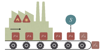
Figure 1: Basic setup of weakly coherent collisional models. The system is allowed to interact sequentially with a series of independent ancillae prepared in states $\rho_{A}$ which are close to being thermal, but have a small amount of coherence [cf. Eq. (5)].

When the ancillae are prepared in thermal states, it is possible to address quantitatively quantities of key thermodynamic relevance, from work to heat currents and entropy Lorenzo et al. (2015a, b); Pezzutto et al. (2016, 2019); Cusumano et al. (2018). This includes both the stroboscopic case, where formal relations can be drawn with the resource theory of athermality Brandão et al. (2013, 2015), and the continuous-time limit Strasberg et al. (2017); Santos et al. (2019). The framework is also readily extended to systems coupled to multiple baths in an entirely consistent way Barra (2015); De Chiara et al. (2018); Pereira (2018). Conversely, when the state of the ancillae is not thermal, much less can be said about its thermodynamic properties.

An important contribution in this direction was given in Ref. Strasberg et al. (2017); Manzano et al. (2018), which put forth a general framework for describing the thermodynamics of collisional models. However, for general ancillary states, the second law of thermodynamics is expressed in terms of system-ancilla correlations and the changes in the state of the ancillae [cf. Eq. (3) below]. These quantities are rarely accessible in practice, which greatly limits the operational use of such formulations.

Motivated by this search for “thermodynamics beyond thermal states”, in this paper we draw a theoretical formulation of the laws of thermodynamics for the class of weakly coherent collisional models (Fig. 1), i.e. situations where the ancillae are prepared in states that, albeit close to thermal ones, retain a small amount of coherence. This is a realistic case, as perfect thermal equilibrium is unlikely to be achieved in practice.

We show that, despite their weakness, the implications of such residual coherence for both the first and second law of thermodynamics are striking, in that non-trivial contributions to the continuous-time open dynamics arise to affect the phenomenology of energy exchanges between system and environment Lorenzo et al. (2015a). In order to illustrate these features in a clear manner, we choose a scenario where no work is externally performed on the global system-ancilla compound Barra (2015); De Chiara et al. (2018); Pereira (2018), so that all changes in the energy of the system can be faithfully attributed to heat flowing from or into the environment. Despite this, we derive a bound showing how coherence in the ancillae (quantified by the relative entropy of coherence) is consumed to convert part of the heat into a coherent (work-like) term in the system.

Our analysis thus entails that quantum coherence can embody a faithful resource in the energetics of open quantum systems Santos et al. (2019). Such resource can be consumed to transform disordered energy (heat) into ordered one (work), thus catalyzing the interconversion of thermodynamic energy exchanges of profoundly different nature, and paving the way to the control and steering of the thermodynamics of quantum processes.

Collisional models - We begin by describing the general structure of collisional models. A system $S$ interacts with an arbitrary number of environmental ancillae $A_{1}$, $A_{2},\ldots$, all identically prepared in a certain state $\rho_{A}$. Each system-ancilla interaction lasts for a time $\tau$ and is governed by a unitary $U_{SA_{n}}$. The state of $S$ after its interaction with $A_{n}$ is embodied by the stroboscopic map

$$\rho_{S}((n+1)\tau)=\operatorname{tr}_{A_{n}}\left(\rho^{\prime}_{SA_{n}}\right)\equiv\operatorname{tr}_{A_{n}}\left[U_{SA_{n}}\left(\rho_{S}(n\tau)\otimes\rho_{A}\right)U_{SA_{n}}^{\dagger}\right],$$ (1)

where $\rho_{S}(n\tau)$ is the state of $S$ before the $n^{\rm th}$ system-ancilla interaction.

Next, let $H_{S}$ and $H_{A_{n}}$ denote the free Hamiltonians of the system and ancillae. We define the heat exchanged in each interaction as the change in energy in the state of the ancilla Reeb and Wolf (2014); Talkner et al. (2009); Goold et al. (2015) $Q_{A_{n}}=\operatorname{tr}\big{\{}H_{A_{n}}(\rho_{A_{n}}^{\prime}-\rho_{A_{n}})\big{\}}$, where $\rho_{A_{n}}^{\prime}=\operatorname{tr}_{S}\rho_{SA_{n}}^{\prime}$. Work is then defined as the mismatch between $Q_{A_{n}}$ and the change in energy of the system, $\Delta E_{n}=\operatorname{tr}\big{\{}H_{S}\big{[}\rho_{S}((n+1)\tau)-\rho_{S}(n\tau)\big{]}\big{\}}$, leading to the usual first law of thermodynamics

$$\Delta E_{n}=W_{n}-Q_{A_{n}}.$$ (2)

As the global dynamics is unitary, the definition of work in this case is unambiguous, being associated with the cost of switching the $S$-$A_{n}$ interaction on and off Barra (2015); De Chiara et al. (2018); Pereira (2018). This work cost will be strictly zero whenever the system satisfies the condition Brandão et al. (2013, 2015) $[U_{SA_{n}},H_{S}+H_{A_{n}}]=0$, which states strict energy conservation. In this case, Eq. (2) reduces to $\Delta E_{n}=-Q_{A_{n}}$, which implies that all energy changes in the system can be unambiguously attributed to energy flowing to or from the ancillae. In order to highlight the role of quantum coherence, we shall assume this is the case throughout the paper. The extension to the case where work is also present is straightforward.

The second law of thermodynamics for the map in Eq. (1) can be expressed as the positivity of the entropy production in each stroke, defined as Strasberg et al. (2017); Manzano et al. (2018)

$$\Sigma_{n}=\mathcal{I}(\rho_{SA_{n}}^{\prime})+S(\rho^{\prime}_{A_{n}}||\rho_{A_{n}}),$$ (3)

where $\mathcal{I}(\rho_{SA_{n}}^{\prime})=S(\rho_{S}^{\prime})+S(\rho_{A_{n}}^{\prime})-S(\rho_{SA_{n}}^{\prime})$ is the mutual information between $S$ and $A_{n}$ after their joint evolution, $S(\rho_{A_{n}}^{\prime}||\rho_{A_{n}})=\operatorname{tr}\big{(}\rho_{A_{n}}^{\prime}\ln\rho_{A_{n}}^{\prime}-\rho_{A_{n}}^{\prime}\ln\rho_{A_{n}}\big{)}$ is the relative entropy between the initial and final states of $A_{n}$, and $S(\rho)=-\operatorname{tr}\left(\rho\ln\rho\right)$ is the von Neumann entropy. Eq. (3) quantifies the degree of irreversibility associated with tracing out the ancillae. It accounts not only for the system-ancilla correlations that are irretrievably lost in this process, but also for the change in state of the ancilla, represented by the last term in Eq. (3). The two terms were recently compared in Refs. Ptaszynski and Esposito (2019b); Pezzutto et al. (2016), and in the context of Landauer’s principle Reeb and Wolf (2014).

Continuous-time limit - In the limit of small $\tau$, Eq. (1) can be approximated by a Lindblad master equation. Such a limit requires a value of $\tau$ sufficiently small to allow us to approximate $\rho_{S}((n+1)\tau)-\rho_{S}(n\tau)$ as a sufficiently smooth derivative. Mathematically, in order to implement this, it is convenient to rescale the interaction potential $V_{SA_{n}}$ between $S$ and $A_{n}$ by a factor $1/\sqrt{\tau}$ Englert and Morigi (2002); Karevski and Platini (2009); Landi et al. (2014). That is, one assumes that the total $S$-$A_{n}$ Hamiltonian is of the form

$$H_{SA_{n}}=H_{S}+H_{A_{n}}+V_{SA_{n}}/\sqrt{\tau}$$ (4)

with the unitary evolution $U_{SA_{n}}=\exp[-i\tau H_{SA_{n}}]$. This kind of rescaling, which enables the performance of the continuous-time limit, is frequent in stochastic processes; e.g.  in classical Brownian motion or in the interaction with the radiation field Ciccarello (2017).

Weakly coherent ancillae - Finally, we specify the state of the ancillae, which is the main feature of our construction. We assume that the ancillae are prepared in a state of the form

$$\rho_{A}=\rho_{A}^{\text{th}}+\sqrt{\tau}\;\lambda\chi_{A},$$ (5)

where $\rho_{A}^{\text{th}}={e^{-\beta H_{A}}}/{Z_{A}}$ is a thermal state at the inverse temperature $\beta$ ($Z_{A}$ is the corresponding partition function). Here $\chi_{A}$ is a Hermitian operator having no diagonal elements in the energy basis of $H_{A}$. Moreover, $\lambda$ is a control parameter that measures the magnitude of the coherences. Notice that the term “weak coherences” is used here in the sense that we are interested specifically in the case where $\tau\to 0$, in which case the second term in (5) is much smaller in magnitude than the first. For finite $\tau$, not all choices of $\chi_{A}$ lead to a positive semidefinite $\rho_{A}$. However, in the limit $\tau\to 0$, these constraints are relaxed and any form of $\chi_{A}$ having no diagonal entries becomes allowed.

The scaling in Eq. (5) highlights an interesting feature of coherent collisional models, namely that for a short $\tau$ and strong $V_{SA_{n}}$, even weak coherences already produce non-negligible contributions.

We use the unitary $U_{SA_{n}}$ generated by Eq. (4) and the state in Eq. (5) in the map stated in Eq. (1). We then expand the latter in power series of $\tau$ and take the limit $\tau\to 0$. This then leads to the quantum master equation (cf. Sup for details)

$$\dot{\rho}_{S}=-i[H_{S}+\lambda\;G,\rho_{S}]+D(\rho_{S}),$$ (6)

where $\dot{\rho}_{S}=\lim_{\tau\to 0}\big{[}\rho_{S}((n+1)\tau)-\rho_{S}(n\tau)\big{]}/\tau$. We also define

$$D(\rho_{S})=-\operatorname{tr}_{A}[V_{SA},[V_{SA},\rho_{S}\otimes\rho_{A}^{\text{th}}]]/2,$$ (7)

representing the usual Lindblad dissipator associated with the thermal part $\rho_{A}^{\text{th}}$, and

$$G=\operatorname{tr}_{A}(V_{SA}\chi_{A})$$ (8)

representing a new unitary contribution stemming from the coherent part of $\rho_{A}$. In deriving Eq. (6) we have assumed that $\operatorname{tr}_{A}(V_{SA}\rho_{A}^{\text{th}})=0$, as customary Rivas and Huelga (2012). Eqs. (6)-(8) provide a general recipe for deriving quantum master equations in the presences of weak coherences. All one requires is the form of the system-ancilla interaction potential and the state of the ancillae. In the limit $\lambda\to 0$ one recovers the standard thermal master equation Englert and Morigi (2002); Karevski and Platini (2009); Landi et al. (2014); De Chiara et al. (2018).

Eigenoperator interaction - The physics of Eqs. (6)-(8) becomes clearer if one assumes a specific form for the interaction $V_{SA}$. A structure which is particularly illuminating, in light of the strict energy-conservation condition, is

$$V_{SA}=\sum\limits_{k}g_{k}L_{k}^{\dagger}A_{k}+h.c.,$$ (9)

where $g_{k}$ are complex coefficients and $L_{k}$ and $A_{k}$ are eigenoperators for the system and ancilla respectively Breuer and Petruccione (2007). That is, they satisfy the conditions $[H_{S},L_{k}]=-\omega_{k}L_{k}$ and $[H_{A},A_{k}]=-\omega_{k}A_{k}$, for the same set of Bohr frequencies $\{\omega_{k}\}$. This means that they function as lowering and raising operators for the energy basis of $S$ and $A$. As both have the same $\omega_{k}$, all of the energy leaving the system enters an ancilla and viceversa, so that strict energy conservation is always satisfied.

The form taken by the dissipator in Eq. (7) when $V_{SA}$ is as given above is the standard thermal one

$$D(\rho_{S})=\sum\limits_{k}\bigg{\{}\gamma_{k}^{-}\mathcal{D}[L_{k}]+\gamma_{k}^{+}\mathcal{D}[L_{k}^{\dagger}]\bigg{\}},$$ (10)

where $\mathcal{D}[L]=L\rho_{S}L^{\dagger}-\frac{1}{2}\{L^{\dagger}L,\rho\}$. We also define the jump coefficients $\gamma_{k}^{-}=|g_{k}|^{2}\langle A_{k}A_{k}^{\dagger}\rangle_{\text{th}}$ and $\gamma_{k}^{+}=|g_{k}|^{2}\langle A_{k}^{\dagger}A_{k}\rangle_{\text{th}}$, with $\langle\ldots\rangle_{\text{th}}=\operatorname{tr}\big{\{}(\ldots)\rho_{A}^{\text{th}}\big{\}}$. As shown e.g. in Ref. Breuer and Petruccione (2007), since the $A_{k}$ are eigenoperators, these coefficients satisfy detailed balance $\gamma_{k}^{+}/\gamma_{k}^{-}=e^{-\beta\omega_{k}}$. As for the new coherent contribution in Eq. (8), we now find

$$G=\sum\limits_{k}\bigg{\{}g_{k}\langle A_{k}\rangle_{\chi}L_{k}^{\dagger}+g_{k}^{*}\langle A_{k}^{\dagger}\rangle_{\chi}L_{k}\bigg{\}},$$ (11)

where $\langle\ldots\rangle_{\chi}=\operatorname{tr}\big{\{}(\ldots)\chi\big{\}}$ means an average over the coherent part $\chi$ of the ancillae.

Qubit example - As an illustrative example, suppose both system and ancillae are resonant qubits with $H_{S(A)}=\frac{\Omega}{2}\sigma_{z}^{S(A)}$ and $V_{SA}=g(\sigma_{+}^{S}\sigma_{-}^{A}+\sigma_{-}^{S}\sigma_{+}^{A})$. Moreover, we take $\chi_{A}=|0\rangle\langle 1|+|1\rangle\langle 0|$, so that Eq. (10) reduces to the simple amplitude damping dissipator $D(\rho_{S})=\sum_{j=\pm}\gamma^{j}\mathcal{D}[\sigma_{j}^{S}]$, whereas the coherent contribution in Eq. (11) goes to $G=g\sigma_{x}^{S}$. The dynamics of the system will then mimic that of a two-level atom driven by classical light, with $D(\rho_{S})$ representing the incoherent emission or absorption of radiation and $G$ a coherent driving term.

Modified first law - Collisional models enable the unambiguous distinctions between heat and work, which is in general not the case Alicki (1979), due to the full access to the global dynamics offered by such approaches Strasberg et al. (2017); De Chiara et al. (2018). In particular, Eq. (6) was derived under the assumption of strong energy conservation, so that no work by an external agent is required to perform the unitary. Any energy changes in the system are thus solely due to energy leaving or entering the ancillae.

The evolution of $\langle H_{S}\rangle$ is easily evaluated as

$${d\langle H_{S}\rangle}/{dt}=i\lambda\langle[G,H_{S}]\rangle+\operatorname{tr}\left[H_{S}D(\rho_{S})\right].$$ (12)

The basic structure of these two terms is clearly different. The second term represents the typical incoherent energy usually associated with heat, whereas the first represents a coherent contribution more akin to quantum mechanical work. Indeed, we show below that, the first term in Eq. (12) satisfies the properties expected from quantum mechanical work. We shall thus refer to it as the coherent work, $\dot{\mathcal{W}}_{C}=i\lambda\langle[G,H_{S}]\rangle$. We also refer to the last term in Eq. (12) as the incoherent heat, $\dot{\mathcal{Q}}_{\text{inc}}=\operatorname{tr}\big{\{}H_{S}D(\rho_{S})\big{\}}$. As the ancillas are not thermal, they will act as both thermal and work reservoirs (in the sense specified in Ref. Strasberg et al. (2017)). As a consequence, classifying their change of energy as heat or work is prone to a certain level of ambiguity. For weakly coherent ancillas, however, this separation becomes unambiguous.

Combining this with Eq. (2) gives the modified first law

$${d\langle H_{S}\rangle}/{dt}\equiv-\dot{Q}_{A}=\dot{\mathcal{W}}_{C}+\dot{\mathcal{Q}}_{\text{inc}},$$ (13)

where $\dot{Q}_{A}=\lim_{\tau\to 0}Q_{A_{n}}/\tau$ is the change in energy of each ancilla. Such modified first law is one of our key results. It reflects a transformation process, where part of the heat flowing in or out of the ancillae is converted into a coherent energy change $\mathcal{W}_{C}$, with the remainder staying as the incoherent heat $\dot{\mathcal{Q}}_{\text{inc}}$. Next, we show that this transformation process is made possible by consuming coherence in the ancillae.

Modified second law - We now turn to the second law in Eq. (3). All entropic quantities can be computed using perturbation theory in $\tau$, leading to results that become exact in the limit $\tau\to 0$. The details are given in Ref. Sup . We find rCl I(ρ_SA_n’) &= -βΔF - ΔC_A_n
S(ρ^′_A_n——ρ_A) = βW_C + ΔC_A_n, where $\Delta F$ is the change in non-equilibrium free energy of the system, $F(\rho_{S})=\langle H_{S}\rangle-TS(\rho_{S})$ and $\mathcal{W}_{C}\simeq\dot{\mathcal{W}}_{C}\tau$. Moreover $\Delta C_{A_{n}}=C(\rho^{\prime}_{A_{n}})-C(\rho_{A_{n}})$ is the change in the relative entropy of coherence Baumgratz et al. (2014); Streltsov et al. (2017) in the state of the ancillae with $\mathcal{C}(\rho_{A})=S(\rho_{A}^{d})-S(\rho_{A})$, with $\rho_{A}^{d}$ the diagonal part of $\rho_{A}$ in the eigenbasis of $H_{A}$. If $\lambda=0$ in Eq. (5), we get $\mathcal{W}_{C}=\Delta C_{A_{n}}=0$ (so that $\Sigma=-\beta\Delta F$).

The positivity of the relative entropy in Eq. (1) implies that in each system-ancilla interaction, the coherent work is always bounded by

$$\beta\mathcal{W}_{C}\geq-\Delta C_{A_{n}}.$$ (14)

This is the core result of our investigation: It shows that the coherent work is bounded by the loss of coherence in the state of the ancillae, which needs to be consumed in order to enable the transformation process described in Eq. (13). Coherence can, in this case, therefore be interpreted as a thermodynamic resource, which must be used to convert disordered energy in the ancillae into an ordered type of energy usable for the system.

On a more general level, the resource in question here is the athermality of $\rho_{A}$ Brandão et al. (2013, 2015); Lostaglio et al. (2015) (i.e., its non-passive character Uzdin and Rahav (2018)). However, the specifics of how this resource can be extracted (which requires knowledge of the operator $G$) and, most importantly, into what it can be converted too, will depend on the form of $\rho_{A}$. This argument can be further strengthened by studying the ergotropy Allahverdyan et al. (2004) in the state (5). This is defined as the maximum amount of work extractable from $\rho_{A}$. As we show in Sup , for weakly coherent states it follows that $\mathcal{W}=TC(\rho_{A})$. This provides additional physical grounds to the bound in Eq. (14): the optimal process for extracting coherent work is when the ancillas lose all their coherence, so that $-\Delta C(\rho_{A})=C(\rho_{A})$.

Inserting Eqs. (1) and (1) in Eq. (3) and taking the limit $\tau\to 0$, one finds that the entropy production rate $\Pi=\lim_{\tau\to 0}\Sigma_{n}/\tau$ can be expressed as

$$\Pi=\beta\left(\dot{\mathcal{W}}_{C}-\dot{F}\right)=\dot{S}(\rho_{S})-\beta\dot{\mathcal{Q}}_{\text{inc}}.$$ (15)

This equation embodies a modified second law of thermodynamics in the presence of weak coherences.It is structurally identical to the classical second law Fermi (1956), but with the coherent work $\mathcal{W}_{C}$ instead. The positivity of $\Pi$ sets the bound $\dot{\mathcal{W}}_{C}\geq\dot{F}$ that, albeit looser than the one in Eq. (14), has the advantage of depend solely on system-related quantities.

Extension to multiple environments - An extremely powerful feature of collisional models is the ability to describe systems coupled to multiple baths. The typical idea is represented in Fig. 2. The system is placed to interact with multiple species of ancillae, with each species being independent and identically prepared in states $\rho_{A}$, $\rho_{B}$, $\rho_{C}$, etc. This can be used to model non-equilibrium steady-states, e.g. of systems coupled to multiple baths. In the stroboscopic scenario the state of the system will be constantly bouncing back and forth with each interaction, even in the long-time limit. But the stroboscopic state after sequences of repeated interactions with the ancillae will in general converge to a steady-state.

The remarkable feature of this construction is that the contributions from each species become additive in the continuous-time limit, in contrast to models where the bath is constantly coupled to the system Mitchison and Plenio (2018). We assume that each interaction lasts for a time $\tau/m$, where $m$ is the number of ancilla species (e.g. $m=3$ in Fig. 2). Moreover, let $i=A,B,C,\ldots,m$ label the different species. To obtain a well behaved continuous-time limit, one must rescale the interaction potential $V_{Si}$ with each species [Eq. (4)] by $m/\sqrt{\tau}$, while keeping the coherent terms in Eq. (5) proportional to $\sqrt{\tau}$. Using this recipe we find the master equation

$$\dot{\rho}=-i\big{[}H_{S}+\sum_{j}\lambda_{j}G_{Sj},\rho_{S}\big{]}+\sum\limits_{j}D_{j}(\rho_{S}),$$ (16)

where the sums are over the various species involved, while $G_{Sj}$ and $D_{j}$ are exactly the same as those given in Eqs. (7) and (8). This is extremely useful, as it provides a recipe to construct complex master equations, with non-trivial steady-states, from fundamental underlying building blocks.

This approach translates neatly into the first and second laws of thermodynamics, which now become

$${d\langle H_{S}\rangle}/{dt}\equiv-\sum\limits_{j}\dot{Q}_{j}=\sum\limits_{j}\left(\dot{\mathcal{W}}_{C}^{j}+\dot{\mathcal{Q}}_{\text{inc}}^{j}\right),$$ (17)

and

$$\Pi=\dot{S}(\rho_{S})-\sum\limits_{j}\beta_{j}\dot{\mathcal{Q}}_{\text{inc}}^{j},$$ (18)

where $\beta_{j}$ is the inverse temperature of species $j$. Both have the same structure as the usual first and second laws for systems coupled to multiple environments.

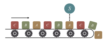
Figure 2: Example of a collisional model where the system interacts with multiple species of ancillae.

Conclusions - We have introduced a scenario beyond the standard system plus thermal-bath, for which operationally useful thermodynamic laws can be constructed. The key feature of our scenario is the use of weakly coherent states. For strong system-ancilla interactions, even weak coherences already lead to a non-trivial contribution. This leads to a modified continuous-time Lindblad master equation that encompasses a non-trivial coherent term giving rise to an effective work contribution to the energetics of the open system, although no external work is exerted at the global level. Incoherent (thermal) energy provided by the environment is catalyzed into work-like terms for the system to use by the (weak) coherence with which the former is endowed.

We believe that this analysis thus provides a striking example of the resource-like role that coherence can play in non-equilibrium thermodynamic processes Santos et al. (2019). This could find applications, for instance, in the design of heat engines mixing classical and quantum resources.

Acknowledgements.– The authors acknowledge fruitful discussions with E. Lutz, A. C. Michels, J. P. Santos. FLSR acknowledges support from the Brazilian funding agency CNPq. GTL acknowledges the São Paulo Research Foundation (FAPESP) under grant numbers 2018/12813-0, 2017/50304-7. MP is supported by the EU Collaborative project TEQ (grant agreement 766900), the DfE-SFI Investigator Programme (grant 15/IA/2864), COST Action CA15220, the Royal Society Wolfson Research Fellowship ((RSWF\R3\183013), and the Leverhulme Trust Research Project Grant (grant nr. RGP-2018-266). GTL and MP are grateful to the SPRINT programme supported by FAPESP and Queen’s University Belfast.

In this supplemental material we provide additional details on the mathematical derivations of our most relevant results. In Sec. S1 we discuss the derivation of Eq. (6) of the main text. In Sec. S2 we discuss how to use perturbation theory to compute the von Neumann entropy and related quantities. These are then used in Sec. S3 to derive Eqs. (1) and (1) of the main text.

I S1. Derivation of Eq. (6) of the main text

The derivation of Eq. (6) is straightforward once the basic ingredients are properly defined. We consider for simplicity a single system-ancilla interaction event. The system is prepared in an arbitrary state $\rho_{S}$, whereas the ancilla is prepared in the weakly coherent state $\rho_{A}$ in Eq. (5) of the main text. We then apply the unitary $U_{SA}$ generated by the Hamiltonian (4). A Baker-Campbell-Haussdorf series expansion in $\tau$ leads to

$$\rho_{SA}^{\prime}=\rho_{S}\rho_{A}-i\tau[H_{SA},\rho_{S}\rho_{A}]-\frac{\tau^{2}}{2}[H_{SA},[H_{SA},\rho_{S}\rho_{A}]].$$ (S1)

Using the specific scalings of $V_{SA}$ and $\rho_{A}$, and keeping only terms at most linear in $\tau$ we get

$$\rho_{SA}^{\prime}=\rho_{S}\rho_{A}-i\tau[H_{S}+H_{A},\rho_{S}\rho_{A}]-i\sqrt{\tau}\;[V_{SA},\rho_{S}\rho_{A}]-\frac{\tau}{2}[V_{SA},[V_{SA},\rho_{S}\rho_{A}^{\text{th}}]]+\mathcal{O}(\tau)^{3/2}.$$ (S2)

In the last term we neglected a contribution from the coherent part $\chi_{A}$, as this would lead to a term at least of order $\tau^{3/2}$. However, in the firs two terms we kept the full $\rho_{A}=\rho_{A}^{\text{th}}+\sqrt{\lambda^{2}\tau}\chi_{A}$.

Eq. (6) of the main text now follows directly by taking the trace of Eq. (S2) over $A$ and assuming that $\operatorname{tr}_{A}(V_{SA}\rho_{A}^{\text{th}})=0$, which leads to

$${\rho_{S}^{\prime}=\rho_{S}-i\tau[H_{S},\rho_{S}]-i\lambda\tau[G,\rho_{S}]+\tau D(\rho_{S}),}$$ (S3)

with $D$ and $G$ given in Eqs. (7) and (8) of the main text. Dividing both sides by $\tau$ and defining

$$\frac{d\rho_{S}}{dt}=\lim\limits_{\tau\to 0}\frac{\rho_{S}^{\prime}-\rho_{S}}{\tau},$$ (S4)

then leads to Eq. (6).

Below we will also need the updated state of the ancillae, after they have interacted with the system. This can be obtained by taking the partial trace of Eq. (S2) over $S$. Keeping only terms which are at most linear in $\tau$, we find

$${\rho_{A}^{\prime}=\rho_{A}^{\text{th}}+\sqrt{\tau}\bigg{(}\lambda\chi_{A}-i[G_{A},\rho_{A}^{\text{th}}]\bigg{)}+\tau\bigg{(}-i\lambda[G_{A},\chi_{A}]+D_{A}(\rho_{A}^{\text{th}})\bigg{)}.}$$ (S5)

where rCl G_A &= tr_S (V_SA ρ_S),
D_A(ρ_A^th) = -12 tr_S [V_SA, [V_SA, ρ_S ρ_A^th]]. Quite relevant to the discussion below, the term of order $\sqrt{\tau}$ does not vanish in Eq (S5).

Energy balance

Using the general map (S1) we can compute the changes in energy of the system and ancilla, defined as $\Delta H_{S}=\operatorname{tr}\big{\{}H_{S}(\rho_{SA}^{\prime}-\rho_{S}\rho_{A})\big{\}}$ and $\Delta H_{A}=\operatorname{tr}\big{\{}H_{A}(\rho_{SA}^{\prime}-\rho_{S}\rho_{A})\big{\}}$. One then readily finds rCl ΔH_S &= i τ ⟨[V_SA, H_S] ⟩_SA - τ2 ⟨[V_SA, [V_SA, H_S]] ⟩_SA,
ΔH_A = i τ ⟨[V_SA, H_A] ⟩_SA - τ2 ⟨[V_SA, [V_SA, H_A]] ⟩_SA. where $\langle\ldots\rangle_{SA}$ means averages over $\rho_{S}\rho_{A}$. In writing these formulas, we have not yet specified the state $\rho_{A}$ in order to emphasize the fact that the structure of these results is entirely independent of it. Due to strong energy conservation, $[V_{SA},H_{S}+H_{A}]=0$ it follows that rCl ⟨[V_SA, H_S] ⟩_SA &= - ⟨[V_SA, H_A] ⟩_SA,
⟨[V_SA, [V_SA, H_S]] ⟩_SA = -⟨[V_SA, [V_SA, H_A]] ⟩_SA, and hence

$$\Delta H_{S}=-\Delta H_{A}.$$ (S6)

Two conclusions may be drawn from this. The first is that, as mentioned in the main text, the strong energy conservation condition (4) implies that no work is performed; all change in energy in the system stems from a corresponding change in the ancillae. Second, Eqs. (I) and (I) allow us to pinpoint the origin of the coherent work $\mathcal{W}_{C}$ and the incoherent heat $\mathcal{Q}_{\text{inc}}$ appearing in Eq. (12) of the main text.

To accomplish this, we simply need to express global averages over $\rho_{S}\rho_{A}$ in terms of local averages over either $\rho_{S}$ or $\rho_{A}$. For instance, referring to Eq. (I), the first term is precisely the coherent work since

$$\mathcal{W}_{C}=i\lambda\tau\langle[G,H_{S}]\rangle_{S}=i\sqrt{\tau}\langle[V_{SA},H_{S}]\rangle_{SA}.$$

The identity in Eq. (I) therefore implies that this contribution will stems from a corresponding term on the side of the ancilla of the form $\langle[V_{SA},H_{A}]\rangle$. Whence,

$$\mathcal{W}_{C}=-i\sqrt{\tau}\langle[V_{SA},H_{A}]\rangle_{SA}=-i\sqrt{\tau}\langle[G_{A},H_{A}]\rangle_{A},$$ (S7)

where $G_{A}$ is given in Eq. (S5). In the last term, the average over $\rho_{A}^{\text{th}}$ does not contribute, so we finally get

$$\mathcal{W}_{C}=-i\lambda\tau\langle[G_{A},H_{A}]\rangle_{\chi_{A}}.$$ (S8)

Similarly, the incoherent heat $\mathcal{Q}_{\text{inc}}$ is related to the second term in Eq. (I):

$$\mathcal{Q}_{\text{inc}}=\tau\operatorname{tr}\bigg{\{}H_{S}D(\rho_{S})\bigg{\}}=-\frac{\tau}{2}\langle[V_{SA},[V_{SA},H_{S}]]\rangle=\frac{\tau}{2}\langle[V_{SA},[V_{SA},H_{A}]]\rangle=-\tau\operatorname{tr}\bigg{\{}H_{A}D_{A}(\rho_{A}^{\text{th}})\bigg{\}},$$ (S9)

where $D_{A}(\rho_{A}^{\text{th}})=-\frac{1}{2}\operatorname{tr}_{S}[V_{SA},[V_{SA},\rho_{S}\rho_{A}^{\text{th}}]]$. The total change in energy of the system, which is the heat leaving the ancilla, can then be written solely in terms of ancilla-based quantities:

$${\Delta\langle H_{S}\rangle:=-Q_{A}=\mathcal{W}_{C}+\mathcal{Q}_{\text{inc}}=-i\lambda\tau\langle[G_{A},H_{A}]\rangle_{\chi_{A}}-\tau\operatorname{tr}\bigg{\{}H_{A}D_{A}(\rho_{A}^{\text{th}})\bigg{\}}.}$$ (S10)

These results therefore allow us to pinpoint which terms in the heat $\Delta H_{A}$ leaving the ancilla are converted to $\mathcal{W}_{C}$ and $\mathcal{Q}_{\text{inc}}$.

II S2. Perturbative expansion of entropic quantities

The states of system and ancilla, before and after the interactions, will generally depend on $\tau$ in different ways. To compute the entropy production, defined in Eq (3) of the main text, one must compute several entropic quantities depending on these states. Since we are interested in the limit $\tau\to 0$, these quantities can be computed using perturbation theory, which becomes exact in the limit $\tau\to 0$. In this section we start by stating some general results on perturbative expansions of the von Neumann entropy, the relative entropy of coherence and the quantum Kullback-Leibler divergence (relative entropy). In Sec. S3 we will then specialize these results to the relevant states appearing in Eq. (3) and derive the results in Eqs. (1) and (1).

II.1 Von Neumann entropy

Consider a general density matrix of the form

$$\rho=\rho_{0}+\epsilon\sigma,$$ (S11)

where $\epsilon$ is a small parameter and we assume $\operatorname{tr}\rho_{0}=1$ so $\operatorname{tr}\sigma=0$. Let $\rho_{0}=\sum_{i}p_{i}|i\rangle\langle i|$ denote the eigendecomposition of the unperturbed density matrix $\rho_{0}$. We now wish to compute the von Neumann entropy of $\rho$, which reads

$$S(\rho)=-\operatorname{tr}(\rho\ln\rho)=-\sum\limits_{i}P_{i}\ln P_{i},$$ (S12)

where $P_{i}$ are the eigenvalues of the full density matrix $\rho$.

Since $\rho$ is a Hermitian operator, standard perturbation theory applies Chen (2010). Assuming that the $p_{i}$ are non-degenerate, we may then write, up to order $\epsilon^{2}$,

$$P_{i}=p_{i}+\epsilon\sigma_{ii}+\epsilon^{2}\sum\limits_{j\neq i}\frac{|\sigma_{ij}|^{2}}{p_{i}-p_{j}}.$$ (S13)

Plugging this in Eq. (S12), expanding $P_{i}\ln P_{i}$ in $\epsilon$ up to second order and using the fact that $\operatorname{tr}\sigma=0$, we find that

$${S(\rho)=S(\rho_{0})-\epsilon\sum\limits_{i}\sigma_{ii}\ln p_{i}-\epsilon^{2}\sum\limits_{i}\bigg{\{}\frac{\sigma_{ii}^{2}}{2p_{i}}+\sum\limits_{j\neq i}\frac{|\sigma_{ij}|^{2}}{p_{i}-p_{j}}\ln p_{i}\bigg{\}}.}$$ (S14)

This is the series expansion for $S(\rho)$. The populations $\sigma_{ii}$ contribute both with order $\epsilon$ and $\epsilon^{2}$, whereas the coherences (off-diagonals) only start to contribute at order $\epsilon^{2}$.

II.2 Relative entropy of coherence

Due to this separation, the relative entropy of coherence [cf. the definition below Eq. (15) of the main text] will be of order $\epsilon^{2}$:

$$\mathcal{C}(\rho)=\epsilon^{2}\sum\limits_{i,j\neq i}\frac{|\sigma_{ij}|^{2}}{p_{i}-p_{j}}\ln p_{i}.$$ (S15)

This expression can also be written more symmetrically, as

$$\mathcal{C}(\rho)=\frac{\epsilon^{2}}{2}\sum\limits_{i,j\neq i}\frac{|\sigma_{ij}|^{2}}{p_{i}-p_{j}}\ln p_{i}/p_{j}.$$ (S16)

Thus, we see that the relative entropy of coherence weights each coherence $|\sigma_{ij}|$ by a factor of the form

$$\frac{\ln(x/y)}{x-y}\geq 1,\qquad x,y\in[0,1].$$

II.3 Quantum relative entropy

Next we consider the relative entropy $S(\rho^{\prime}||\rho)$ between two density matrices of the form

$$\rho=\rho_{0}+\epsilon\sigma,\qquad\rho^{\prime}=\rho_{0}+\epsilon\mu,$$ (S17)

where $\sigma$ and $\mu$ are arbitrary, but both depend on $\rho_{0}$ to order $\epsilon^{0}$. We have

$$S(\rho^{\prime}||\rho)=-S(\rho^{\prime})-\operatorname{tr}(\rho^{\prime}\ln\rho).$$ (S18)

The first term was already found in (S14), with $\sigma$ replaced by $\mu$:

$$S(\rho^{\prime})=S(\rho_{0})-\epsilon\sum\limits_{i}\mu_{ii}\ln p_{i}-\epsilon^{2}\sum\limits_{i}\bigg{\{}\frac{\mu_{ii}^{2}}{2p_{i}}+\sum\limits_{j\neq i}\frac{|\mu_{ij}|^{2}}{p_{i}-p_{j}}\ln p_{i}\bigg{\}}.$$ (S19)

In order to compute the last term we will need not only the perturbation theory for the eigenvalues of $\rho$ [Eq. (S13)], but also for its eigenvectors. Defining $\rho=\sum\limits_{i}P_{i}|\tilde{i}\rangle\langle\tilde{i}|$ allows us to write

$$\operatorname{tr}(\rho^{\prime}\ln\rho)=\sum\limits_{i}\langle\tilde{i}|\rho^{\prime}|\tilde{i}\rangle\ln P_{i}.$$ (S20)

Thus, in addition to writing $\ln P_{i}$ as a power series, we will also have to expand $\langle\tilde{i}|\rho^{\prime}|\tilde{i}\rangle$.

Using standard perturbation theory, the eigenvectors of $\rho$ can be written as

$$|\tilde{i}\rangle=|i\rangle+\epsilon|i_{1}\rangle+\epsilon^{2}|i_{2}\rangle,$$ (S21)

where rCl —i_1⟩&= ∑_j≠i —j⟩σijpi- pj,
—i_2⟩= - 12 —i⟩∑_j≠i —σij—2(pi- pj)2 - ∑_j≠i —j⟩σiiσji(pi- pj)2 +∑_j≠i, k ≠i —k⟩σkjσji(pi-pj)(pi-pk) With this we find, after carrying out the computations,

$$\langle\tilde{i}|\rho^{\prime}|\tilde{i}\rangle=p_{i}+\epsilon\mu_{ii}+\epsilon^{2}\sum\limits_{j\neq i}\frac{\mu_{ij}\sigma_{ji}+\sigma_{ij}\mu_{ji}-|\sigma_{ij}|^{2}}{p_{i}-p_{j}}.$$ (S22)

Plugging this result in Eq. (S20) and expanding all terms in $\epsilon$ then finally leads to

$$\operatorname{tr}(\rho^{\prime}\ln\rho)=\sum\limits_{i}\Bigg{\{}p_{i}\ln p_{i}+\epsilon(\sigma_{ii}+\mu_{ii}\ln p_{i})+\epsilon^{2}\bigg{[}\frac{\mu_{ii}\sigma_{ii}}{p_{i}}-\frac{\sigma_{ii}^{2}}{2p_{i}}+\sum\limits_{j\neq i}\frac{\mu_{ij}\sigma_{ji}+\sigma_{ij}\mu_{ji}-|\sigma_{ij}|^{2}}{p_{i}-p_{j}}\ln p_{i}\bigg{]}\Bigg{\}},$$ (S23)

which is correct up to order $\epsilon^{2}$. Finally, combining this with Eq. (S19) leads to

$${S(\rho^{\prime}||\rho)=\frac{\epsilon^{2}}{2}\sum\limits_{i}\Bigg{\{}\frac{(\mu_{ii}-\sigma_{ii})^{2}}{p_{i}}+\sum\limits_{j\neq i}\frac{|\mu_{ij}-\sigma_{ij}|^{2}}{p_{i}-p_{j}}\ln(p_{i}/p_{j})\Bigg{\}}.}$$ (S24)

We therefore see that while $S(\rho)$ and $S(\rho^{\prime})$ contain contributions of order $\epsilon$, the first non-zero contribution to the relative entropy is of order $\epsilon^{2}$. Moreover, the result depends on both the populations and the coherences, and both with the same order $\epsilon^{2}$. This highlights some of the differences between $S(\rho^{\prime}||\rho)$ and $S(\rho^{\prime})-S(\rho)$.

III S3. Calculation of $\mathcal{I}(\rho_{SA}^{\prime})$ and $S(\rho_{A}^{\prime}||\rho_{A})$ [Eqs. (1) and (1) of the main text]

We are now in the position to derive Eqs. (1) and (1) of the main text. To do so, one must simply apply the results of Sec. S2 with the appropriate choices of $\rho$, $\rho_{0}$, etc. Since system and environment always start uncorrelated and since the global dynamics is unitary, the mutual information developed in the map (S1) can be written as

$$\mathcal{I}(\rho_{SA}^{\prime})=S(\rho_{S}^{\prime})+S(\rho_{A}^{\prime})-S(\rho_{SA}^{\prime}):=\Delta S_{S}+\Delta S_{A}.$$ (S25)

Our task is to compute $\Delta S_{A}=S(\rho_{A}^{\prime})-S(\rho_{A})$. In addition, we will also need $S(\rho_{A}^{\prime}||\rho_{A})$. We compute each term separately.

III.1 Calculation of $S(\rho_{A})$

The initial state of the ancilla is given in Eq. (5) of the main text, $\rho_{A}=\rho_{A}^{\text{th}}+\sqrt{\lambda^{2}\tau}\chi_{A}$, where $\chi_{A}$ has no diagonal elements. This falls under the structure of Eq. (S11), provided we identify

$$\epsilon\sigma=\sqrt{\tau}\lambda\chi_{A}.$$

A direct application of Eq. (S14) then yields

$$S(\rho_{A})=S(\rho_{A}^{\text{th}})-\lambda^{2}\tau\sum\limits_{i,j\neq i}\frac{|(\chi_{A})_{ij}|^{2}}{p_{i}^{\text{th}}-p_{j}^{\text{th}}}\ln p_{i}^{\text{th}},$$ (S26)

where $p_{i}^{\text{th}}$ are the eigenvalues of $\rho_{A}^{\text{th}}$ and the basis $|i\rangle$ refers to the energy basis of $H_{A}$. Since the perturbed part of $\rho_{A}$ has no diagonal elements, the second term in Eq. (S26) is nothing but the relative entropy of coherence of the state $\rho_{A}$,

$$C(\rho_{A})=\lambda^{2}\tau\sum\limits_{i,j\neq i}\frac{|(\chi_{A})_{ij}|^{2}}{p_{i}^{\text{th}}-p_{j}^{\text{th}}}\ln p_{i}^{\text{th}}.$$ (S27)

Thus, we may simply write

$${S(\rho_{A})=S(\rho_{A}^{\text{th}})-C(\rho_{A}).}$$ (S28)

III.2 Calculation of $S(\rho_{A}^{\prime})$

The state of the ancilla after the map is given by Eq. (S5). This once again has the structure Eq. (S11), but now one must identify

$$\epsilon\sigma=\sqrt{\tau}\bigg{\{}\lambda\chi_{A}-i[G_{A},\rho_{A}^{\text{th}}]\bigg{\}}+\tau\bigg{\{}-i\lambda[G_{A},\chi_{A}]+D_{A}(\rho_{A}^{\text{th}})\bigg{\}}.$$

The terms proportional to $\sqrt{\tau}$ now form the off-diagonal part of $\sigma$ and those proportional to $\tau$ are all diagonal. Applying again Eq. (S14) yields

$$S(\rho_{A}^{\prime})=S(\rho_{A}^{\text{th}})-\tau\sum\limits_{i}\bigg{(}-i\lambda[G_{A},\chi_{A}]+D_{A}(\rho_{A}^{\text{th}})\bigg{)}_{ii}\ln p_{i}^{\text{th}}-\tau\sum\limits_{i,j\neq i}\frac{\bigg{|}\bigg{(}\lambda\chi_{A}-i[G_{A},\rho_{A}^{\text{th}}]\bigg{)}_{ij}\bigg{|}^{2}}{p_{i}^{\text{th}}-p_{j}^{\text{th}}}\ln p_{i}^{\text{th}}.$$

Once again, comparing with Eqs. (S14) and (S15), the relative entropy of coherence of $\rho_{A}^{\prime}$ corresponds to the last term only,

$$C(\rho_{A}^{\prime})=\tau\sum\limits_{i,j\neq i}\frac{\bigg{|}\bigg{(}\lambda\chi_{A}-i[G_{A},\rho_{A}^{\text{th}}]\bigg{)}_{ij}\bigg{|}^{2}}{p_{i}^{\text{th}}-p_{j}^{\text{th}}}\ln p_{i}^{\text{th}}.$$ (S29)

That is, we may write

$$S(\rho_{A}^{\prime})=S(\rho_{A}^{\text{th}})-\tau\sum\limits_{i}\bigg{(}-i\lambda[G_{A},\chi_{A}]+D_{A}(\rho_{A}^{\text{th}})\bigg{)}_{ii}\ln p_{i}^{\text{th}}-C(\rho_{A}^{\prime}).$$

The term proportional to $\tau$, on the other hand, can be written as

$$-\tau\sum\limits_{i}\bigg{(}-i\lambda[G_{A},\chi_{A}]+D_{A}(\rho_{A}^{\text{th}})\bigg{)}_{ii}\ln p_{i}^{\text{th}}=\beta\tau\operatorname{tr}_{A}\bigg{\{}\bigg{(}-i\lambda[G_{A},\chi_{A}]+D_{A}(\rho_{A}^{\text{th}})\bigg{)}H_{A}\bigg{\}},\$$

where we also use the fact that $\ln\rho_{A}^{\text{th}}=-\beta H_{A}-\ln Z_{A}$ [c.f. Eq. (5) of the main text]. The terms proportional to $\ln Z_{A}$ vanish since the operators in the above expression are all traceless. This term is therefore nothing but the total change in energy of the ancilla in Eq. (S10). But this, in turn, is minus the change in energy in the system. Whence, we conclude that

$${S(\rho_{A}^{\prime})=S(\rho_{A}^{\text{th}})-\beta\Delta\langle H_{S}\rangle-C(\rho_{A}^{\prime}).}$$ (S30)

III.3 Calculation of $\mathcal{I}(\rho_{SA}^{\prime})$

Inserting Eqs. (S28) and (S30) into Eq. (S25) leads to

$${\mathcal{I}(\rho_{SA}^{\prime})=\Delta S_{S}-\beta\Delta\langle H_{S}\rangle-\Delta C_{A},}$$ (S31)

which is Eq. (1) of the main text, provided we recognize $\Delta S_{S}-\beta\Delta\langle H_{S}\rangle=-\beta\Delta F$, as the change in free energy of the system.

III.4 Calculation of $S(\rho_{A}^{\prime}||\rho_{A})$

Finally, we turn to the relative entropy $S(\rho_{A}^{\prime}||\rho_{A})$, expressed as the series in Eq. (S24). The operators $\mu$ and $\sigma$, defined in Eq. (S17), should now be recognized with rCl ϵσ&= τ λχ_A,
ϵμ= τ{λχ_A - i [G_A, ρ_A^th] } + τ{ - i λ[G_A, χ_A] + D_A(ρ_A^th)}. The first term in Eq. (S24) will depend only on the diagonal part of $\mu$ (the diagonal part of $\sigma$ is zero). But this term is already of order $\tau$, so this will ultimately lead to a contribution of order $\tau^{2}$.

The only non-negligible term is thus the one related to the coherences. It is convenient to express $|\mu_{ij}-\sigma_{ij}|^{2}$ as

$$|\mu_{ij}-\sigma_{ij}|^{2}=|\mu_{ij}|^{2}-|\sigma_{ij}|^{2}+\bigg{(}2|\sigma_{ij}|^{2}-\mu_{ij}\sigma_{ji}-\sigma_{ij}\mu_{ji}\bigg{)}.$$

The reason why this is useful is because then the first two terms can be recognized as the difference between the relative entropies of coherence of $\rho_{A}^{\prime}$ and $\rho_{A}$ respectively [Eqs. (S29) and (S27)]. On the other hand, the remaining term in parenthesis may be written as

$$2|\sigma_{ij}|^{2}-\mu_{ij}\sigma_{ji}-\sigma_{ij}\mu_{ji}=i\lambda\bigg{[}(\chi_{A})_{ij}(G_{A})_{ji}-(G_{A})_{ij}(\chi_{A})_{ji}\bigg{]}(p_{i}^{\text{th}}-p_{j}^{\text{th}}).$$

Substituting these results in Eq. (S24) and expressing the remaining summations in terms of a trace, then yields

$$S(\rho_{A}^{\prime}||\rho_{A})=\Delta C_{A}-i\lambda\beta\tau\langle[G_{A},H_{A}]\rangle_{\chi_{A}}.$$

Comparing this with Eq. (S8), we finally arrive at Eq. (1) of the main text; viz.,

$${S(\rho_{A}^{\prime}||\rho_{A})=\Delta C_{A}+\beta\mathcal{W}_{C}.}$$ (S32)

IV S4. Ergotropy

Using the results of Sec. S.2 it is straightforward to compute the ergotropy of the ancilla state $\rho_{A}$ (see main text for discussions). To conform with the notation of Sec. S.2., let us study instead the state (S11), but assuming that $\rho_{0}$ is a thermal state $\rho_{0}=e^{-\beta H}/Z$, with population $p_{i}=e^{-\beta E_{i}}/Z$ and eigenbasis $|i\rangle$. Matching this to the notation of the ancilla state $\rho_{A}$ [Eq. (5) of the main text] will be straightforward once the final result has been derived.

The ergotropy is defined as (Ref. Allahverdyan et al. (2004) of the main text)

$$\mathcal{W}=\sum\limits_{ij}P_{i}E_{j}\bigg{[}|\langle j|\tilde{i}\rangle|^{2}-\delta_{ij}\bigg{]}.$$ (S33)

Here $P_{i}$ and $|\tilde{i}\rangle$ are the eigenvalues and eigenvectors of $\rho$, which are given by Eqs. (S13) and (S21) respectively. Using the fact that $\langle i|i_{1}\rangle=0$ [c.f. Eq. (S21)], it follows that

$$|\langle j|\tilde{i}\rangle|^{2}=\delta_{ij}+\epsilon^{2}\bigg{[}|\langle j|i_{1}\rangle|^{2}+2\delta_{ij}\text{Re}(\langle i|i_{2}\rangle)\bigg{]},$$

which is thus already of order $\epsilon^{2}$. We now plug this in Eq. (S33). Restricting the calculation only up to $\epsilon^{2}$, as was done in the previous sections, we see that we only need to take the zeroth order term of $P_{i}$ [Eq. (S13)], which is precisely the equilibrium probabilities $p_{i}$. Whence, Eq. (S33) becomes

$$\mathcal{W}=\epsilon^{2}\sum\limits_{ij}p_{i}E_{j}\bigg{[}|\langle j|i_{1}\rangle|^{2}+2\delta_{ij}\text{Re}(\langle i|i_{2}\rangle)\bigg{]}.$$

From (S21) and (S21) we get rCl —⟨j — i_1 ⟩—^2 &= (1-δ_ij) —σij—2(pi- pj)2,
2 Re(⟨i — i_2 ⟩) = - ∑_j≠i —σij—2(pi- pj)2. This allows us to write

$$\mathcal{W}=\epsilon^{2}\sum\limits_{i,j\neq i}p_{i}(E_{j}-E_{i})\frac{|\sigma_{ij}|^{2}}{(p_{i}-p_{j})^{2}}.$$

Finally, we write $E_{j}-E_{i}=T\ln p_{i}/p_{j}$ and also symmetrize the formula, exactly as was done in going from Eq. (S15) to (S16). We then finally get

$$\mathcal{W}=\frac{T\epsilon^{2}}{2}\sum\limits_{i,j\neq i}\frac{|\sigma_{ij}|^{2}}{(p_{i}-p_{j})}\ln p_{i}/p_{j}=TC(\rho),$$ (S34)

where the connection with the relative entropy of coherence $C(\rho)$ can be directly verified by comparing with Eq. (S16). Translating this now to the weakly coherent state of the ancilla [Eq. (5) of the main text], one concludes that the ergotropy contained in $\rho_{A}$ is simply $\mathcal{W}=TC(\rho_{A})$.

References

- Scully et al. (2007) M. O. Scully, M. S. Zubairy, and G. S. Agarwal, Science 862, 862 (2007).
- Dillenschneider and Lutz (2009) R. Dillenschneider and E. Lutz, European Physics Letters 88, 50003 (2009).
- Gardas and Deffner (2015) B. Gardas and S. Deffner, Physical Review E 92, 042126 (2015).
- Manzano et al. (2016) G. Manzano, F. Galve, R. Zambrini, and J. M. R. Parrondo, Physical Review E 93, 052120 (2016).
- Manzano (2018) G. Manzano, Physical Review E 98, 042123 (2018), arXiv:1806.07448 .
- Rossnagel et al. (2014) J. Rossnagel, O. Abah, F. Schmidt-Kaler, K. Singer, and E. Lutz, Physical Review Letters 112, 030602 (2014), arXiv:1308.5935 .
- Manzano et al. (2019) G. Manzano, R. Silva, and J. M. R. Parrondo, Physical Review E 99, 042135 (2019), arXiv:1709.00231 .
- Ptaszynski and Esposito (2019a) K. Ptaszynski and M. Esposito, Physical Review Letters 122, 150603 (2019a), arXiv:1901.01093 .
- Holmes et al. (2018) Z. Holmes, S. Weidt, D. Jennings, J. Anders, and F. Mintert, Quantum 3, 124 (2018), arXiv:1806.11256 .
- Korzekwa et al. (2016) K. Korzekwa, M. Lostaglio, J. Oppenheim, and D. Jennings, New Journal of Physics 18, 023045 (2016).
- Bäumer et al. (2019) E. Bäumer, M. Lostaglio, M. Perarnau-Llobet, and R. Sampaio, in Thermodynamics in the quantum regime - Fundamental Theories of Physics, edited by F. Binder, L. Correa, C. Gogolin, J. Anders, and G. Adesso (Springer, 2019) p. 195, arXiv:1805.10096 .
- Micadei et al. (2019) K. Micadei, J. P. S. Peterson, A. M. Souza, R. S. Sarthour, I. S. Oliveira, G. T. Landi, T. B. Batalhão, R. M. Serra, and E. Lutz, Nature Communications 10, 2456 (2019), arXiv:1711.03323 .
- Klaers et al. (2017) J. Klaers, S. Faelt, A. Imamoglu, and E. Togan, Physical Review X 7, 031044 (2017), arXiv:1703.10024 .
- Scarani et al. (2002) V. Scarani, M. Ziman, P. Štelmachovič, N. Gisin, V. Bužek, and V. Bužek, Physical Review Letters 88, 097905 (2002), arXiv:0110088 [quant-ph] .
- Ziman et al. (2002) M. Ziman, P. Štelmachovič, V. Buzžek, M. Hillery, V. Scarani, and N. Gisin, Physical Review A. Atomic, Molecular, and Optical Physics 65, 042105 (2002).
- Karevski and Platini (2009) D. Karevski and T. Platini, Physical Review Letters 102, 207207 (2009), arXiv:0904.3527 .
- Giovannetti and Palma (2012) V. Giovannetti and G. M. Palma, Physical Review Letters 108, 040401 (2012).
- Landi et al. (2014) G. T. Landi, E. Novais, M. J. de Oliveira, and D. Karevski, Physical Review E 90, 042142 (2014).
- Strasberg et al. (2017) P. Strasberg, G. Schaller, T. Brandes, and M. Esposito, Physical Review X 7, 021003 (2017), arXiv:1610.01829 .
- Barra (2015) F. Barra, Scientific Reports 5, 14873 (2015), arXiv:1509.04223 .
- Pereira (2018) E. Pereira, Physical Review E 97, 022115 (2018).
- Lorenzo et al. (2015a) S. Lorenzo, R. McCloskey, F. Ciccarello, M. Paternostro, and G. Palma, Physical Review Letters 115, 120403 (2015a), arXiv:arXiv:1503.07837v2 .
- Lorenzo et al. (2015b) S. Lorenzo, A. Farace, F. Ciccarello, G. M. Palma, and V. Giovannetti, Physical Review A 91, 022121 (2015b).
- Pezzutto et al. (2016) M. Pezzutto, M. Paternostro, and Y. Omar, New Journal of Physics 18, 123018 (2016).
- Pezzutto et al. (2019) M. Pezzutto, M. Paternostro, and Y. Omar, Quantum Science and Technology 4, 025002 (2019), arXiv:1806.10075 .
- Cusumano et al. (2018) S. Cusumano, V. Cavina, M. Keck, A. De Pasquale, and V. Giovannetti, Physical Review A 98, 032119 (2018), arXiv:arXiv:1807.04500v2 .
- Englert and Morigi (2002) B.-G. Englert and G. Morigi, in Coherent Evolution in Noisy Environments - Lecture Notes in Physics, edited by A. Buchleitner and K. Hornberger (Springer, Berlin, Heidelberg, 2002) p. 611, arXiv:0206116 [quant-ph] .
- Doob (1954) J. L. Doob, in Selected Papers on Noise and Stochastic Processes, edited by N. Wax (Dover, New York, 1954).
- Brandão et al. (2013) F. G. S. L. Brandão, M. Horodecki, J. Oppenheim, J. M. Renes, and R. W. Spekkens, Physical Review Letters 111, 250404 (2013), arXiv:1111.3882 .
- Brandão et al. (2015) F. G. S. L. Brandão, M. Horodecki, N. H. Y. Ng, J. Oppenheim, and S. Wehner, Proceedings of the National Academy of Sciences 112, 3275 (2015), arXiv:1305.5278 .
- Santos et al. (2019) J. P. Santos, L. C. Céleri, G. T. Landi, and M. Paternostro, Nature Quantum Information (accepted) 5, 23 (2019), arXiv:1707.08946 .
- De Chiara et al. (2018) G. De Chiara, G. Landi, A. Hewgill, B. Reid, A. Ferraro, A. J. Roncaglia, and M. Antezza, New Journal of Physics 20, 113024 (2018), arXiv:1808.10450 .
- Manzano et al. (2018) G. Manzano, J. M. Horowitz, and J. M. R. Parrondo, Physical Review X 8, 031037 (2018), arXiv:1710.00054 .
- Reeb and Wolf (2014) D. Reeb and M. M. Wolf, New Journal of Physics 16, 103011 (2014), arXiv:1306.4352 .
- Talkner et al. (2009) P. Talkner, M. Campisi, and P. Hänggi, Journal of Statistical Mechanics: Theory and Experiment 2009, P02025 (2009).
- Goold et al. (2015) J. Goold, M. Paternostro, and K. Modi, Physical Review Letters 114, 060602 (2015).
- Ptaszynski and Esposito (2019b) K. Ptaszynski and M. Esposito, (2019b), arXiv:1905.03804 .
- Note (1) For instance, the white noise appearing in the Langevin equation of Brownian motion acts for an infinitesimal time so, in order to be non-trivial, it has to also be infinitely strong Coffey et al. (2004).
- Ciccarello (2017) F. Ciccarello, Quantum Measurements and Quantum Metrology 4, 53 (2017), arXiv:1712.04994 .
- (40) See supplemental material.
- Rivas and Huelga (2012) Á. Rivas and F. S. Huelga, Open quantum systems: an introduction (Springer, Heidelberg, 2012).
- Breuer and Petruccione (2007) H. P. Breuer and F. Petruccione, The Theory of Open Quantum Systems (Oxford University Press, USA, 2007) p. 636.
- Alicki (1979) R. Alicki, Journal of Physics A: Mathematical and General 12, L103 (1979).
- Baumgratz et al. (2014) T. Baumgratz, M. Cramer, and M. B. Plenio, Physical Review Letters 113, 140401 (2014), arXiv:1311.0275 .
- Streltsov et al. (2017) A. Streltsov, G. Adesso, and M. B. Plenio, Reviews of Modern Physics 89, 041003 (2017), arXiv:1609.02439 .
- Lostaglio et al. (2015) M. Lostaglio, D. Jennings, and T. Rudolph, Nature communications 6, 6383 (2015), arXiv:1405.2188 .
- Uzdin and Rahav (2018) R. Uzdin and S. Rahav, Physical Review X 8, 021064 (2018), arXiv:1805.00220 .
- Allahverdyan et al. (2004) A. E. Allahverdyan, R. Balian, and T. M. Nieuwenhuizen, Europhysics Letters 67, 565 (2004), arXiv:0401574 [cond-mat] .
- Fermi (1956) E. Fermi, Thermodynamics (Dover Publications Inc., 1956) p. 160.
- Mitchison and Plenio (2018) M. T. Mitchison and M. B. Plenio, New Journal of Physics 20, 033005 (2018), arXiv:1708.05574 .
- Coffey et al. (2004) W. T. Coffey, Y. P. Kalmykov, and J. T. Waldron, The Langevin Equation. With Applications to Stochastic Problems in Physics, Chemistry and Electrical Engineering, 2nd ed. (World Scientific Publishing Co, Pte. Ltd., Singapore, 2004) p. 678.
- Chen (2010) X. Y. Chen, Chinese Physics B 19, 1 (2010), arXiv:0902.4733 .
Supplemental Material