Modifying AMG coarse spaces with weak approximation property to exhibit approximation in energy norm

Abstract

Algebraic multigrid (AMG) coarse spaces are commonly constructed so that they exhibit the so-called weak approximation (WAP) property which is necessary and sufficient condition for uniform two-grid convergence. This paper studies a modification of such coarse spaces so that the modified ones provide approximation in energy norm. Our modification is based on the projection in energy norm onto an orthogonal complement of original coarse space. This generally leads to dense modified coarse space matrices which is hence computationally infeasible. To remedy this, based on the fact that the projection involves inverse of a well-conditioned matrix, we use polynomials to approximate the projection and, therefore, obtain a practical, sparse modified coarse matrix and prove that the modified coarse space maintains computationally feasible approximation in energy norm. We present some numerical results for both, PDE discretization matrices as well as graph Laplacian ones, which are in accordance with our theoretical results.

65F10, 65N20, 65N30

1 Introduction

Algebraic multigrid is one of the most successful methods for solving large-scale sparse systems of linear equations $A{\mathbf{u}}={\mathbf{f}}$ with symmetric positive definite (SPD) matrix $A$, especially for the case when $A$ comes from finite element discretization of second order elliptic equations. AMG has also been extended to matrices arising from much broader classes of discretized PDEs (e.g., [24], the AMS and ADS solvers in [14], [15]) and even for non-PDE matrices (using adaptive AMG, see e.g., [4, 8]), including ones coming from network simulations (e.g. graph Laplacian, [20]). For an overview of some AMG methods, we refer to [28] and more recently to [29].

Another important aspect of AMG, which is the main focus of this work, is that it provides a hierarchy of coarse spaces, which are natural candidates for dimension reduction, sometimes referred to as numerical upscaling. There are quite a few literature on multigrid-based upscaling techniques, e.g., [11, 21, 23], and domain-decomposition-based upscaling approaches, e.g., [18, 26]. However, one difficulty, which needs to be overcome with such an approach, is that the traditional AMG coarse spaces can not guarantee the required approximation accuracy. More precisely, by the construction, traditional AMG coarse spaces only guarantee to possess a so-called weak approximation property (WAP), i.e., for any vector ${\mathbf{u}}\in\mathbb{R}^{n}$, there exists a vector ${\mathbf{u}}_{c}$ belonging to the coarse space, such that $\|{\mathbf{u}}-P{\mathbf{u}}_{c}\|_{D}\leq\eta_{w}\|{\mathbf{u}}\|_{A}$, where $\|{\mathbf{u}}\|_{A}:=\sqrt{{\mathbf{u}}^{T}A{\mathbf{u}}}$ is the so-called energy norm and $\|{\mathbf{u}}\|_{D}:=\sqrt{{\mathbf{u}}^{T}D{\mathbf{u}}}$ is the (weighted) $\ell_{2}$-norm induced by a proper chosen SPD matrix $D$. The WAP is known to be necessary and sufficient for the uniform convergence of the two-level AMG methods (cf., e.g., [28]). However, to use the same coarse space for dimension reduction, we need that the Galerkin projection (projection with respect to energy norm $\|\cdot\|_{A}$) onto the coarse space exhibit some approximation property. A sufficient condition is that the coarse spaces satisfy the so-called strong approximation property (SAP), i.e., the coarse-level solution should approximate the original (fine-level) solution with some guaranteed accuracy in energy norm. Mathematically, the SAP means that, for any vector ${\mathbf{u}}\in\mathbb{R}^{n}$, there exists a vector ${\mathbf{u}}_{c}$ belonging to the coarse space, such that $\|A\|\|{\mathbf{u}}-P{\mathbf{u}}_{c}\|^{2}_{A}\leq\eta_{s}\|A{\mathbf{u}}\|^{2}$. Although the AMG coarse spaces do have approximation properties (by construction, in a weighted $\ell_{2}$-norm), the coarse-level solution (i.e., the computationally feasible Galerkin projection) does not generally possess that, neither in (weighted) $\ell_{2}$-norm nor in energy norm $\|\cdot\|_{A}$. To the best of our knowledge, none of the existing multigrid- and domain decomposition-based upscaling techniques have the desired SAP property with provable satisfactory bound on the resulting constant $\eta_{s}$.

In this paper, we address the issue that the usual AMG coarse spaces do not satisfy the SAP with provable satisfactory bound on the resulting constant $\eta_{s}$ and develop an approach by extending a construction originated in [22] to our more general AMG upscaling setting. Our main contribution, which distinguish our result from all the existing results, is that our modified coarse space satisfies the SAP with provable satisfactory bound on the resulting constant $\eta_{s}$, which provides computable approximation to the fine-level solution in both the energy norm and (weighted) $\ell_{2}$-norm. The proposed method simply modifies the AMG coarse space $\operatorname{Range}(P)$ ($P$ is the prolongation matrix which satisfies the WAP by construction/assumption) to $\operatorname{Range}((I-\pi_{f})P)$ where $\pi_{f}$ is a projection onto the $A$-orthogonal complement of $\operatorname{Range}(P)$ (i.e., orthogonal complement of $\operatorname{Range}(P)$ with respect to the $A$ inner product ${\mathbf{u}}^{T}A{\mathbf{v}}$). We show that such modified coarse space provides a two-level $A$-orthogonal decomposition of the original fine-level solution ${\mathbf{u}}$ and, thereby, energy error estimate of the coarse solution. Moreover, the SAP of the coarse space can be derived based on such decomposition as well. Details of the construction of $\pi_{f}$ will be presented in Section 3. Because the definition of $\pi_{f}$ involves the inverse of a matrix (see Section 2.3 for details), such modification typically leads to dense coarse matrices which is mostly of theoretical interest. In order to design a more practical approach, we take advantage of the fact that $A$ is well-conditioned on the $A$-orthogonal complement of $\operatorname{Range}(P)$ (which we prove holds for $P$ satisfying the WAP) and, therefore, modifying the coarse spaces based on polynomial approximations to control the sparsity of the respective coarse matrices is feasible. That is, we are able to modify the coarse space so that both, the SAP (hence the error estimate in the energy norm) and the sparsity of the coarse matrix, are satisfied. The energy error estimate improves when the polynomial degree increases (with the expense of increased matrix density). We present numerical results illustrating the effectiveness of the proposed method. We would like to point out that other computationally feasible AMG-type upscaling approaches were presented in [1] and [13] for problems that can be formulated in a mixed (saddle-point) form.

The remainder of the paper is structured as follows. In Section 2, we introduce the WAP and formulate some properties of the matrices arising from the unsmoothed aggregation AMG. It provides the motivation for the construction of the improved coarse spaces which is presented in Section 3. The error analysis in the computationally infeasible case with exact projections is presented in that section as well. The computationally feasible case with approximate projections, giving rise to the improved coarse space satisfying the SAP and with guaranteed approximation properties is presented in Section 4. The case of elliptic problems with high contrast coefficients is briefly discussed in Section 5. The numerical illustration of the presented methods for both, PDE-type matrices and graph Laplacian ones, can be found in Section 6. Finally, some conclusions are drawn in the last Section 7.

2 Weak approximation property in AMG

In this section, we recall the two-grid method and the weak approximation property that is widely used to prove the convergence of two-grid methods. We point out that the prolongation matrices $P$ constructed in various AMG methods usually satisfy the WAP (a notion intoduced already in the original AMG paper, [2].

We consider a SPD matrix $A\in\mathbb{R}^{n\times n}$ and let $D$ be another SPD matrix such that,

(2.1) $${\mathbf{v}}^{T}A{\mathbf{v}}\leq{\mathbf{v}}^{T}D{\mathbf{v}}.$$

A typical choice of $D$ is the diagonal of $A$ with proper scaling, i.e. $D=\omega^{-1}\,\text{diag}(A)$, $\omega\in\mathbb{R}$ or the so-called “$\ell_{1}$-smoother” (cf. e.g., [5]). We denote the norms induced by $A$ and $D$ by $\|\cdot\|_{A}$ and $\|\cdot\|_{D}$, respectively.

2.1 The two-grid method

First, we briefly recall the standard two-grid method. Assume we have a smoother $M$ such as Jacobi, Gauss-Seidel, etc., a prolongation $P$, and the coarse-grid problem $A_{c}=P^{T}AP$. Based on these standard components, we define the standard (symmetrized) two-grid method in Algorithm 1.

Algorithm 1 Two-grid method

For a current iterate ${\mathbf{u}}$, we perform:

1:  Presmoothing: ${\mathbf{u}}\leftarrow{\mathbf{u}}+M^{-1}({\mathbf{f}}-A{\mathbf{u}})$

2:  Restriction: ${\mathbf{r}}_{c}\leftarrow P^{T}({\mathbf{f}}-A{\mathbf{u}})$

3:  Coarse-grid correction: ${\mathbf{e}}_{c}=A_{c}^{-1}{\mathbf{r}}_{c}$

4:  Prolongation: ${\mathbf{u}}\leftarrow{\mathbf{u}}+P{\mathbf{e}}_{c}$

5:  Postsmoothing: ${\mathbf{u}}\leftarrow{\mathbf{u}}+M^{-T}({\mathbf{f}}-A{\mathbf{u}})$

It is well-known that the two-grid method (Algorithm 1) leads to the composite iteration matrix $E_{TG}$ based on which we define the two-grid operator $B_{TG}$ as follow,

$$I-B_{TG}^{-1}A=E_{TG}=(I-M^{-T}A)(I-PA_{c}^{-1}P^{T}A)(I-M^{-1}A).$$

For the convergence rate of the two-grid method, we have the following two-grid estimates which can be found in Theorem 4.3, [10].

Theorem 2.1.

For $B_{TG}$ and the two-grid error propagation operator $E_{TG}$, we have the sharp estimates

$${\mathbf{v}}^{T}A{\mathbf{v}}\leq{\mathbf{v}}^{T}B_{TG}{\mathbf{v}}\leq K_{TG}{\mathbf{v}}^{T}A{\mathbf{v}}\quad\text{or equivalently}\quad\|E_{TG}\|_{A}=\rho_{TG}:=1-\frac{1}{K_{TG}},$$

where

$$K_{TG}=\max_{{\mathbf{v}}}\min_{{\mathbf{v}}_{c}}\frac{\|{\mathbf{v}}-P{\mathbf{v}}_{c}\|^{2}_{\widetilde{M}}}{\|{\mathbf{v}}\|^{2}_{A}},$$

and ${\widetilde{M}}:=M^{T}(M^{T}+M-A)^{-1}M$ is the symmetrized smoother (starting with $M^{T}$).

2.2 The Weak Approximation Property

In AMG, we construct a prolongation $P\in\mathbb{R}^{n\times n_{c}}$ and the corresponding coarse space $\text{Range}(P)$ which exhibits the WAP. We note that the WAP is a necessary and sufficient condition for uniform two-level AMG convergence (e.g., [28]) and can be stated as, for any vector ${\mathbf{v}}\in{\mathbb{R}}^{n}$, there is a coarse vector ${\mathbf{v}}_{c}\in{\mathbb{R}}^{n_{c}}$, such that

(2.2) $$\|{\mathbf{v}}-P{\mathbf{v}}_{c}\|_{D}\leq\eta_{w}\;\|{\mathbf{v}}\|_{A},$$

where $\eta_{w}$ is the so-called WAP constant. By requiring that the smoother is spectrally equivalent to $D$, which can be verified for standard smoothers such as Gauss-Seidel and Jacobi, we can estimate the two-grid constant $K_{TG}$ based on the WAP. More precisely, we have $K_{TG}\leq c\eta^{2}_{w}$ where the constant $c$ here measures the spectral equivalence between $\widetilde{M}$ and $D$. This implies that $\rho_{TG}\leq 1-\frac{1}{c\eta_{w}^{2}}$, i.e., the corresponding two-grid method converges uniformly.

In order to have a computationally feasible approach (which will become clear later on), in this paper, we follow [5, 27] and assume that $P$ is constructed based on aggregation-based approach (without smoothing). Roughly speaking, we first form a set of aggregates $\{{\mathcal{A}}_{i}\}_{i=1}^{n_{a}}$, which is a nonoverlapping partitioning of the index set $\{1,\;2,\;\dots,\;n\}$, i.e., $\cup_{i=1}^{n_{a}}{\mathcal{A}}_{i}=\{1,\;2,\;\dots,\;n\}$ and ${\mathcal{A}}_{i}\cap{\mathcal{A}}_{j}=\emptyset$, if $i\neq j$. Moreover, we denote the size of ${\mathcal{A}}_{i}$ by $n_{{\mathcal{A}}_{i}}$ which is defined by the cardinality of ${\mathcal{A}}_{i}$. We then solve certain (generalized) eigenvalue problems locally to obtain the local basis $\{{\mathbf{q}}_{{\mathcal{A}}_{i},j}^{c}\}_{j=1}^{n_{i}^{c}}$ for each aggregate ${\mathcal{A}}_{i}$. The overall prolongation is defined as

(2.3) $$P=\begin{pmatrix}P_{{\mathcal{A}}_{1}}&0&\cdots&0\\ 0&P_{{\mathcal{A}}_{2}}&\cdots&\vdots\\ \vdots&\vdots&\ddots&\vdots\\ 0&\cdots&0&P_{{\mathcal{A}}_{n_{a}}}\end{pmatrix}\ \text{with}\ P_{{\mathcal{A}}_{i}}=({\mathbf{q}}_{{\mathcal{A}}_{i},1}^{c},\cdots,{\mathbf{q}}_{{\mathcal{A}}_{i},n_{i}^{c}}^{c}),$$

and, naturally, the coarse space is just $\text{Range}(P)$. The WAP (2.2) can be shown by the properties of the local eigenvalue problems. We refer to [5, 27] for the details. We note that such local spectral construction of $P$ (2.3) dated back to [3] and is also possible for graph Laplacian matrices (see, e.g., [12]).

As already mentioned, a WAP of the above form is a necessary condition for uniform two-level AMG convergence, so we assume (2.2) to hold for a block-diagonal $P$ and a diagonal $D$ (scaled as in (2.1)).

The assumptions on $P$ and $D$ imply that the matrix $P^{T}DP$ is sparse, actually it is block diagonal with each diagonal block corresponding to an aggregate ${\mathcal{A}}_{i}$. Hence, it is easily invertible and the projection $\pi_{D}=P(P^{T}DP)^{-1}P^{T}D$ is sparse, hence computationally feasible. Taking ${\mathbf{v}}_{c}=(P^{T}DP)^{-1}P^{T}D{\mathbf{v}}$ in (2.2), we arrive at the following estimate, which is another way to present the WAP of the coarse space using the projection $\pi_{D}$,

(2.4) $$\|{\mathbf{v}}-\pi_{D}{\mathbf{v}}\|_{D}\leq\eta_{w}\;\|{\mathbf{v}}\|_{A}.$$

As already mentioned, the WAP plays an important role in the convergence analysis of AMG methods. For example, we can derive two-level convergence rate directly from the WAP. However, in this paper, our goal is to take advantage of the WAP and modify the coarse space such that the modified one satisfies not only the WAP but also the so-called strong approximation property. Coarse spaces that satisfy the SAP with provable satisfactory bound on the constant can provide a coarse-level solution which approximates the fine-level solution with guaranteed accuracy in energy norm, and, therefore, are important both theoretically (e.g., in the V-cycle convergence analysis) and practically (e.g., for upscaling).

2.3 The $A$-Orthogonal Complement to $\operatorname{Range}(I-\pi_{D})$

Our modification of the coarse spaces (which will be presented in the next section) uses information from the orthogonal complement $\operatorname{Range}(I-\pi_{D})$. Therefore, in this subsection, we introduce how to construct a sparse linearly independent basis of the space $\operatorname{Range}(I-\pi_{D})$ and how to project a coarse vector onto it.

The construction of the basis of the space $\operatorname{Range}(I-\pi_{D})$ is, of course, not unique. Here, we are looking for a sparse (locally supported) basis due to computational complexity considerations. In the case of aggregation-based AMG, this can be done as follows. On each aggregate ${\mathcal{A}}_{i}$, we select $n^{f}_{i}$ vectors, $\{{\mathbf{q}}^{f}_{{\mathcal{A}}_{i},j}\}^{n^{f}_{i}}_{j=1}$, which are orthonormal with respect to $D_{{\mathcal{A}}_{i}}:=\left.D\right|_{{\mathcal{A}}_{i}}$ and span the $D_{{\mathcal{A}}_{i}}$-orthogonal complement of $\operatorname{Range}(P_{{\mathcal{A}}_{i}})$. Recall that $n_{{\mathcal{A}}_{i}}$ is the size of the aggregates ${\mathcal{A}}_{i}$ and $n_{i}^{c}$ be the number of columns of $P_{{\mathcal{A}}_{i}}$, we choose $n^{f}_{i}$ such that $n_{{\mathcal{A}}_{i}}=n^{c}_{i}+n^{f}_{i}$. It is clear that the vectors ${\mathbf{q}}^{f}_{{\mathcal{A}}_{i},j}$ extended by zero outside ${\mathcal{A}}_{i}$ form a basis of $\operatorname{Range}(I-\pi_{D})$. Introducing the matrix $P_{\perp}$ with the vectors ${\mathbf{q}}^{f}_{{\mathcal{A}}_{i},j}$ as its columns, then we have,

(2.5) $$P^{T}_{\perp}DP=0\text{ and }P^{T}_{\perp}DP_{\perp}=I.$$

Exploiting the local basis of $\operatorname{Range}(I-\pi_{D})$, we project any given vector $P{\mathbf{v}}_{c}\in\text{Range}(P)$ onto the $A$-orthogonal complement of $\operatorname{Range}(I-\pi_{D})$ by solving the following problem: find ${\mathbf{v}}_{f}\in\operatorname{Range}(I-\pi_{D})$, such that

(2.6) $$({\mathbf{w}}_{f})^{T}A{\mathbf{v}}_{f}=({\mathbf{w}}_{f})^{T}AP{\mathbf{v}}_{c},\quad\forall\,{\mathbf{w}}_{f}\in\operatorname{Range}(I-\pi_{D}).$$

Since we have a sparse (computable) basis of $\operatorname{Range}(I-\pi_{D})$ represented by $P_{\perp}$, we can rewrite (2.6) as the following linear system of equations,

(2.7) $$A_{f}{\overline{\mathbf{v}}}_{f}=P^{T}_{\perp}AP{\mathbf{v}}_{c},$$

where $A_{f}=P^{T}_{\perp}AP_{\perp}$ and ${\mathbf{v}}_{f}=P_{\perp}\overline{{\mathbf{v}}}_{f}$. By solving (2.7), we compute the projection ${\mathbf{v}}_{f}=\pi_{f}P{\mathbf{v}}_{c}$. In fact, the matrix representation of $\pi_{f}$ is given by $\pi_{f}=P_{\perp}A^{-1}_{f}P^{T}_{\perp}A$. Note the inverse of $A_{f}$ is involved in the definition of $\pi_{f}$.

We next study the conditioning of $A_{f}$ with the goal to derive computationally feasible (sparse) approximations to its inverse within reasonable computational cost. We have the following main result.

Theorem 2.2.

If the coarse space $\text{Range}(P)$ satisfies the WAP with constant $\eta_{w}$, then the condition number $\kappa(A_{f})$ of $A_{f}$ satisfies $\kappa(A_{f})\leq\eta_{w}^{2}$.

Proof 2.3.

Choose ${\mathbf{v}}={\mathbf{v}}_{f}:=(I-\pi_{D}){\mathbf{v}}$ in (2.4) and (2.1), which leads to the following spectral equivalence relations,

$$\frac{1}{\eta_{w}^{2}}\;{\mathbf{v}}^{T}_{f}D{\mathbf{v}}_{f}\leq{\mathbf{v}}^{T}_{f}A{\mathbf{v}}_{f}\leq{\mathbf{v}}^{T}_{f}D{\mathbf{v}}_{f},\quad\forall\,{\mathbf{v}}_{f}\in\operatorname{Range}(I-\pi_{D}).$$

Equivalently, letting ${\mathbf{v}}_{f}=P_{\perp}{\overline{\mathbf{v}}}_{f}$, using properties (2.5), we have

(2.8) $$\frac{1}{\eta_{w}^{2}}\;{\overline{\mathbf{v}}}^{T}_{f}{\overline{\mathbf{v}}}_{f}\leq{\overline{\mathbf{v}}}^{T}_{f}A_{f}{\overline{\mathbf{v}}}_{f}\leq{\overline{\mathbf{v}}}^{T}_{f}{\overline{\mathbf{v}}}_{f},\quad\forall\,{\overline{\mathbf{v}}}_{f},$$

which implies that the condition number $\kappa(A_{f})$ of $A_{f}$, satisfies $\kappa(A_{f})\leq\eta^{2}_{w}$, which is the desired result.

Remark 2.4.

When the WAP constant $\eta_{w}$ is bounded, especially independent of problem size, then Theorem 2.2 implies that $A_{f}$ is well-conditioned.

Since $A_{f}$ is well-conditioned, $A_{f}^{-1}$ can be accurately approximated by a matrix polynomial $q_{\nu}(A_{f})$ of degree $\nu$. Therefore, to approximate the solution of $A_{f}{\mathbf{x}}_{f}={\mathbf{f}}_{f}$, we can use the representation

$${\mathbf{x}}_{f}=A^{-1}_{f}{\mathbf{f}}_{f}=\left[\left(A^{-1}_{f}-q_{\nu}(A_{f})\right){\mathbf{f}}_{f}+q_{\nu}(A_{f}){\mathbf{f}}_{f}\right].$$

The first term on the right hand side above can be made as small as we want by choosing $q_{\nu}$ appropriately. More precisely, it can be made of order $\epsilon\ll 1$ if we choose the polynomial degree $\nu=\mathcal{O}(\log\,\epsilon^{-1})$ (cf., e.g., [9], or [28], p. 413). We give specific examples of polynomials $q_{\nu}(t)$ in Section 4. By dropping the first term, we get the approximation

(2.9) $${\mathbf{x}}_{f}\approx q_{\nu}(A_{f}){\mathbf{f}}_{f}.$$

An important observation is that, if ${\mathbf{f}}_{f}$ is locally supported (sparse), the above approximation can be kept reasonably sparse. In particular, consider (2.7), i.e., ${\mathbf{f}}_{f}=P_{\perp}^{T}AP{\mathbf{v}}_{c}$, and let ${\mathbf{v}}_{c}$ be one of the unit coordinate vectors, then $P{\mathbf{v}}_{c}$ is a column of $P$ and has local support represented by a corresponding aggregate ${\mathcal{A}}$. Thus, such ${\mathbf{f}}_{f}$ is locally support on ${\mathcal{A}}$ and its immediate neighbors. In this case, the approximation $q_{\nu}(A_{f}){\mathbf{f}}_{f}$ is supported locally. More precisely, its suport depends on the sparsity of $A^{\nu}_{f}$, hence the diameter of the non-zero pattern of $q_{\nu}(A_{f}){\mathbf{f}}_{f}$ can be estimated to be of order $\nu$ times the size of the neighborhood of ${\mathcal{A}}$ and, therefore, can be kept under control when $\nu$ is kept small.

The above approximation is the main motivation for our work. Roughly speaking, such approximation allows us to modify the original coarse space (with the WAP) so that the modified one satisfies the SAP while keeping the sparsity of the modified prolongation under control. In the next two sections, we first introduce the SAP result in the case of exact $A^{-1}_{f}$ and then present the coarse space modification based on the computationally feasible polynomial approximation.

3 The modified coarse space exhibiting the SAP

In this section we define the modified coarse space. The construction presented here goes back to [22]. In this paper, we adopt a matrix-vector presentation and motivate the applicability of the construction in  [22] to our setting of aggregation-based AMG exploiting the well-conditionedness of $A_{f}$ proven in Theorem 2.2. Thereby, we extend the analysis in [22] to our more general (algebraic) setting by showing that the modified coarse spaces satisfy the SAP with provable satisfactory bound on the resulting constant $\eta_{s}$. In the following section, we extend these results to the case of approximate inverses.

3.1 Modification of the Coarse Space

We first recall the projection $\pi_{f}=P_{\perp}A^{-1}_{f}P^{T}_{\perp}A$ which plays an important role in the construction of the modified coarse space. We also recall the original coarse space given by $\operatorname{Range}(P)=\operatorname{Range}(\pi_{D})$. The modified coarse space of our main interest is simply $\operatorname{Range}((I-\pi_{f})\pi_{D})$, or equivalently $\operatorname{Range}((I-\pi_{f})P)$. Naturally, the modified prolongation matrix takes the form $(I-\pi_{f})P$.

Next, we show that we can obtain an A-orthogonal decomposition of any given vector ${\mathbf{u}}$ based on the modified coarse space, which in turn implies the SAP of our main interest. To this end, we first present some properties of the two projections $\pi_{D}$ and $\pi_{f}$ summarized in the following lemma.

Lemma 3.1.

The projections $\pi_{D}$ and $\pi_{f}$ satisfy $\pi_{D}\pi_{f}=0$. In addition, we have that $(I-\pi_{f})\pi_{D}$ is also a projection.

Proof 3.2.

$\pi_{D}\pi_{f}=0$ can be directly verified by $\pi_{D}=P(P^{T}DP)^{-1}P^{T}D$ and $\pi_{f}=P_{\perp}A^{-1}_{f}P_{\perp}^{T}A$. Together with properties (2.5), we have

$$\pi_{D}\pi_{f}=P(P^{T}DP)^{-1}\underbrace{(P^{T}DP_{\perp})}_{=0}A^{-1}_{f}P_{\perp}^{T}A=0.$$

On the other hand, using $\pi_{D}\pi_{f}=0$ and also the fact that $\pi^{2}_{D}=\pi_{D}$, we have

$$\left((I-\pi_{f})\pi_{D}\right)^{2} =(\pi_{D}-\pi_{f}\pi_{D})(\pi_{D}-\pi_{f}\pi_{D})$$

$$\quad=\pi^{2}_{D}-\pi_{f}\pi^{2}_{D}-(\pi_{D}\pi_{f})\pi_{D}+\pi_{f}(\pi_{D}\pi_{f})\pi_{D}$$

$$\quad=\pi_{D}-\pi_{f}\pi_{D}=(I-\pi_{f})\pi_{D},$$

which implies that $(I-\pi_{f})\pi_{D}$ is a projection.

We are now ready to derive our main two-level A-orthogonal decomposition.

Theorem 3.3.

For a given ${\mathbf{u}}$, there exists a ${\mathbf{v}}$, such that

(3.1) $${\mathbf{u}}=(I-\pi_{D}){\mathbf{v}}+(I-\pi_{f})\pi_{D}{\mathbf{u}}.$$

Also, the two components in the above decomposition are $A$-orthogonal.

Proof 3.4.

We begin with the following $A$-orthogonal decomposition

(3.2) $${\mathbf{u}}=(I-\pi_{D}){\mathbf{v}}+{\boldsymbol{\xi}},\text{ where }{\boldsymbol{\xi}}\in\left(\operatorname{Range}(I-\pi_{D})\right)^{\perp_{A}}.$$

Given a ${\mathbf{v}}_{c}$, from the definition of ${\mathbf{v}}_{f}=\pi_{f}P{\mathbf{v}}_{c}$ in (2.6), we have

$${\mathbf{w}}_{f}^{T}A(I-\pi_{f})P{\mathbf{v}}_{c}=0,\text{ for all ${\mathbf{w}}_{f}\in\text{Range}(I-\pi_{D})$}.$$

The latter identity implies that the $A$-orthogonal complement $\left(\operatorname{Range}(I-\pi_{D})\right)^{\perp_{A}}$ of $\text{Range}(I-\pi_{D})$ satisfies the relations

(3.3) $$\left(\operatorname{Range}(I-\pi_{D})\right)^{\perp_{A}}=\operatorname{Range}\left((I-\pi_{f})P\right)=\operatorname{Range}\left((I-\pi_{f})\pi_{D}\right).$$

This means that in (3.2), ${\boldsymbol{\xi}}=(I-\pi_{f})\pi_{D}{\mathbf{w}}$ for some ${\mathbf{w}}$, hence the A-orthogonal decomposition (3.2) can be rewritten as follows,

$${\mathbf{u}}=(I-\pi_{D}){\mathbf{v}}+(I-\pi_{f})\pi_{D}{\mathbf{w}}.$$

Finally, using Lemma 3.1 we have $\pi_{D}{\mathbf{u}}=\pi_{D}(I-\pi_{f})\pi_{D}{\mathbf{w}}=\pi^{2}_{D}{\mathbf{w}}=\pi_{D}{\mathbf{w}}$, which shows  (3.1).

The above A-orthogonal decomposition (3.1) basically provides an energy stable decomposition since

$$\|{\mathbf{u}}\|_{A}^{2}=\|(I-\pi_{D}){\mathbf{v}}\|_{A}^{2}+\|(I-\pi_{f})\pi_{D}{\mathbf{w}}\|_{A}^{2}.$$

This is essential in multilevel analysis. In the following subsections, we prove the SAP for the modified coarse space $\text{Range}((I-\pi_{f})P)$ and also establish our first main error estimates, all based on this decomposition.

3.2 The Strong Approximation Property

In this subsection, we show that the modified coarse space $\operatorname{Range}((I-\pi_{f})P)$ satisfies the SAP with provable satisfactory bound on the constant $\eta_{s}$. To this end, for given ${\mathbf{f}}$, we consider the solution ${\mathbf{u}}$ of the following linear system,

(3.4) $$A{\mathbf{u}}={\mathbf{f}}.$$

The corresponding modified coarse problem (also known as the upscaled problem) reads

(3.5) $$P^{T}(I-\pi_{f})^{T}A(I-\pi_{f})P{\mathbf{u}}_{c}=P^{T}(I-\pi_{f})^{T}{\mathbf{f}}.$$

In order to show the SAP, we are interested in estimating the error ${\mathbf{e}}={\mathbf{u}}-(I-\pi_{f})P{\mathbf{u}}_{c}$ in the energy norm $\|\cdot\|_{A}$, more precisely, the estimate of $\|{\mathbf{u}}-(I-\pi_{f})P{\mathbf{u}}_{c}\|_{A}$ in terms of $\|{\mathbf{f}}\|=\|A{\mathbf{u}}\|$. The main result is formulated in the following theorem.

Theorem 3.5.

Assume the WAP (2.2) holds. Let ${\mathbf{e}}={\mathbf{u}}-(I-\pi_{f})P{\mathbf{u}}_{c}$ be the error between the fine-level solution ${\mathbf{u}}$ of problem (3.4) and the upscaled (coarse) solution ${\overline{\mathbf{u}}}_{c}=(I-\pi_{f})P{\mathbf{u}}_{c}$ of (3.5). Then, the following energy error estimate holds:

(3.6) $$\|{\mathbf{e}}\|_{A}\leq\eta_{w}\|D^{-\frac{1}{2}}A{\mathbf{u}}\|.$$

Proof 3.6.

By the property of the Galerkin projection, we have that ${\mathbf{e}}={\mathbf{u}}-{\overline{\mathbf{u}}}_{c}$ is $A$-orthogonal to $\operatorname{Range}((I-\pi_{f})P)=\operatorname{Range}((I-\pi_{f})\pi_{D})=\left(\operatorname{Range}(I-\pi_{D})\right)^{\perp_{A}}$. Therefore, using the decomposition (3.1), we have

(3.7) $${\mathbf{e}}={\mathbf{u}}-{\overline{\mathbf{u}}}_{c}=(I-\pi_{D}){\mathbf{v}},\,\text{ for some }{\mathbf{v}}.$$

Since ${\overline{\mathbf{u}}}_{c}\in\operatorname{Range}((I-\pi_{f})P)=\left(\operatorname{Range}(I-\pi_{D})\right)^{\perp_{A}}$, we also have

$$\|{\mathbf{e}}\|^{2}_{A}=({\mathbf{u}}-{\overline{\mathbf{u}}}_{c})^{T}A(I-\pi_{D}){\mathbf{v}}=(A{\mathbf{u}})^{T}(I-\pi_{D}){\mathbf{v}}\leq\|D^{-\frac{1}{2}}{\mathbf{f}}\|\|(I-\pi_{D}){\mathbf{v}}\|_{D}.$$

Using the weak approximation property (2.4) for ${\mathbf{v}}:=(I-\pi_{D}){\mathbf{v}}={\mathbf{e}}$, we then obtain

$$\|{\mathbf{e}}\|^{2}_{A}\leq\|D^{-\frac{1}{2}}{\mathbf{f}}\|\eta_{w}\|(I-\pi_{D}){\mathbf{v}}\|_{A}=\eta_{w}\|D^{-\frac{1}{2}}{\mathbf{f}}\|\|{\mathbf{e}}\|_{A},$$

which implies (3.6).

From the energy error estimate (3.6), assuming that $D$ is well-conditioned, we have the following corollary also known as strong approximation property.

Corollary 3.7 (Strong Approximation Property).

We have the following estimate

(3.8) $$\|A\|\|{\mathbf{u}}-{\overline{\mathbf{u}}}_{c}\|^{2}_{A}\leq\|D\|\|{\mathbf{u}}-{\overline{\mathbf{u}}}_{c}\|^{2}_{A}\leq\eta_{s}\;\|A{\mathbf{u}}\|^{2},$$

where $\eta_{s}\leq\|D\|\|D^{-1}\|\eta^{2}_{w}$, which is referred to as the SAP constant. If $D$ is well-conditioned, then $\eta_{s}$ is bounded from above by a constant.

As we have shown, the modified coarse space $\operatorname{Range}(I-\pi_{f})P$ satisfies the SAP with provable satisfactory bound on the constant $\eta_{s}$. However, we want to point out that, the practical usage of this modified coarse space is limited since $\pi_{f}$ involves $A_{f}^{-1}$ which is dense in general. In Section 4, we discuss how to use the polynomial approximation (2.9) to modify the coarse space which can be used in practice with the SAP approximately satisfied.

3.3 A Weighted $\ell_{2}$–Error Estimate

The estimate (3.6) allows us to prove an $\ell_{2}$–error estimate, which is a direct application of the Aubin-Nitsche argument. Let ${\mathbf{e}}={\mathbf{u}}-{\overline{\mathbf{u}}}_{c}$ be the error and consider the following linear system,

$$A{\mathbf{w}}=D{\mathbf{e}}.$$

We have,

$$\|{\mathbf{e}}\|^{2}_{D}={\mathbf{e}}^{T}(D{\mathbf{e}})={\mathbf{e}}^{T}A{\mathbf{w}}.$$

Since ${\mathbf{e}}$ is $A$-orthogonal to the modified coarse space $\operatorname{Range}(I-\pi_{f})\pi_{D}$, we have, for ${\overline{\mathbf{w}}}_{c}=(I-\pi_{f})\pi_{D}{\mathbf{w}}$ ,

$$\|{\mathbf{e}}\|^{2}_{D}={\mathbf{e}}^{T}A({\mathbf{w}}-{\overline{\mathbf{w}}}_{c})\leq\|{\mathbf{e}}\|_{A}\|{\mathbf{w}}-{\overline{\mathbf{w}}}_{c}\|_{A}.$$

Applying estimate (3.6) to the error ${\mathbf{e}}_{\mathbf{w}}:={\mathbf{w}}-{\overline{\mathbf{w}}}_{c}$ leads to

$$\|{\mathbf{e}}\|^{2}_{D}\leq\|{\mathbf{e}}\|_{A}\eta_{w}\|D^{-\frac{1}{2}}A{\mathbf{w}}\|=\eta_{w}\|{\mathbf{e}}\|_{A}\|D^{\frac{1}{2}}{\mathbf{e}}\|=\eta_{w}\|{\mathbf{e}}\|_{A}\|{\mathbf{e}}\|_{D}.$$

This implies the desired weighted $\ell_{2}$-error estimate stated below.

Theorem 3.8.

Let ${\mathbf{e}}={\mathbf{u}}-(I-\pi_{f})\pi_{D}{\mathbf{u}}$ be the error between the solutions of the original fine-level problem (3.4) and the upscaled one (3.5). Then, the following weighted $\ell_{2}$–error estimate holds:

(3.9) $$\|{\mathbf{e}}\|_{D}\leq\eta_{w}\|{\mathbf{e}}\|_{A}\leq\eta^{2}_{w}\|D^{-\frac{1}{2}}A{\mathbf{u}}\|.$$

4 Modified coarse space using approximate inverses

In this section, we discuss how to use approximations to make the modified coarse spaces more practical. The basic idea is based on the well-conditioning of $A_{f}$ as shown in Theorem 2.2 which allows for uniform polynomial approximation (2.9). We argue that such an approximation keeps the sparsity of the modified prolongation matrix under control while maintaining the approximation properties of the modified coarse space reasonably well. These are properties that make the resulting modified coarse spaces appropriate for upscaling as well for efficient use in multigrid methods in practice.

4.1 Modification via Polynomial Approximation

We begin with one possible choice of polynomial approximation. Recall that according to (2.8), the spectrum of $A_{f}$ is contained in $[1/\eta_{w}^{2},1]\subset(0,1]$. Therefore, we want to chose a polynomial $p_{\nu}$ of degree $\nu\geq 1$, such that $p_{\nu}(0)=1$ and $tp^{2}_{\nu}(t)$ has a small maximum norm over the interval $t\in[0,1]$. One choice is the polynomial used in the smoothed aggregation algebraic multigrid (SA-AMG). It is defined via the Chebyshev polynomials of odd degree, $T_{2\nu+1}$, as follows:

(4.1) $$p_{\nu}(t)=\frac{(-1)^{\nu}}{2\nu+1}\frac{T_{2\nu+1}(\sqrt{t})}{\sqrt{t}}.$$

As is well-known (e.g., shown in [6, 28, 12]), this polynomial has the following property

(4.2) $$\max\limits_{t\in(0,1]}\sqrt{t}|p_{\nu}(t)|=\frac{1}{2\nu+1}.$$

Since $p_{\nu}(0)=1$, $p_{\nu}(t)=1-tq_{\nu-1}(t)$, where $q_{\nu-1}$ is a polynomial of degree $\nu-1$. We actually use $q_{\nu-1}(t)$ to approximate $A_{f}^{-1}$, namely

(4.3) $$A_{f}^{-1}\approx{\widetilde{A}}^{-1}_{f}\equiv q_{\nu-1}(A_{f}).$$

By rewriting (4.3), we get

$$I-{\widetilde{A}}^{-1}_{f}A_{f}=I-q_{\nu-1}(A_{f})A_{f}=p_{\nu}(A_{f}).$$

The $A_{f}$-norm of this matrix can be made arbitrarily small as $\nu\rightarrow\infty$ by the property (4.2).

Letting ${\widetilde{\pi}}_{f}:=P_{\perp}{\widetilde{A}}^{-1}_{f}P^{T}_{\perp}A$, we define the modified prolongation matrix ${\widetilde{P}}$ as follows,

(4.4) $${\widetilde{P}}:=(I-{\widetilde{\pi}}_{f})P.$$

The corresponding modified coarse space is $\operatorname{Range}((I-{\widetilde{\pi}}_{f})P)=\operatorname{Range}((I-{\widetilde{\pi}}_{f})\pi_{D})$. Note that, if we choose $\nu$ properly (sufficiently large but fixed), the modified prolongation matrix ${\widetilde{P}}$ stays reasonably sparse and can be used in practice with nearly optimal computational cost.

We notice that, the formula ${\widetilde{P}}=(I-P_{\perp}q_{\nu-1}(A_{f})P^{T}_{\perp}A)P$, somewhat resembles the construction of prolongation matrices used in SA-AMG. More specifically, in SA-AMG, we have ${\widetilde{P}}:=p_{\nu}(D^{-1}A)P$. This observation offers the possibility to construct new SA-AMG methods by choosing simple $P_{\perp}$ (for example, not necessarily spanning the entire complement of $\operatorname{Range}(P)$) so that $A_{f}:=P^{T}_{\perp}AP_{\perp}$ and hence the resulting ${\widetilde{P}}$ and respective modified coarse level matrix ${\widetilde{P}}^{T}A{\widetilde{P}}$ be reasonably sparse.

Remark 4.1.

We may also note that ${\widetilde{P}}=(I-P_{\perp}q_{\nu-1}(A_{f})P^{T}_{\perp}A)P$ resembles the so-called approximate wavelet modified hierarchical basis (AWMHB) method where $P_{\perp}$ (corresponding to the HB) is modified by polynomially based approximate $L_{2}$-projections to exhibit better energy stability (cf. [25] or [28]).

With the approximate modified coarse space, the two-level decomposition can be rewritten in the following perturbation form

(4.5) $${\mathbf{u}}=(I-\pi_{D}){\mathbf{v}}+(I-{\widetilde{\pi}}_{f})\pi_{D}{\mathbf{u}}+({\widetilde{\pi}_{f}}-\pi_{f})\pi_{D}{\mathbf{u}}.$$

Obviously, we do not have $A$-orthogonality anymore. However, as we show later, the first two terms of the decomposition (4.5) are approximately $A$-orthogonal whereas the last term can be made small, which leads to the desired error estimates.

4.2 Approximate Orthogonality

To show that the first two terms of the decomposition (4.5) are approximately $A$-orthogonal, we prove that the two spaces $\operatorname{Range}(P_{\perp})$ ($=\operatorname{Range}(I-\pi_{D})$) and $\operatorname{Range}({\widetilde{P}})$ ($=\operatorname{Range}((I-{\widetilde{\pi}}_{f})\pi_{D})$) are approximately $A$-orthogonal. To this end, we first establish some properties of $\pi_{D}$ and ${\widetilde{\pi}}_{f}$ summarized in the following lemma.

Lemma 4.2.

We have $\pi_{D}{\widetilde{\pi}}_{f}=0$ and that $(I-{\widetilde{\pi}}_{f})\pi_{D}$ is a projection.

Proof 4.3.

The proof is the same as the proof of Lemma 3.1.

Remark 4.4.

Lemma 4.2 actually holds for ${\widetilde{\pi}}_{f}$ obtained by approximating $A_{f}^{-1}$ with any ${\widetilde{A}}^{-1}_{f}$ in the definition of $\pi_{f}$. Therefore, this allows us to use, for example, other polynomials, i.e., not only the SA polynomial (4.1).

Next, we estimate the cosine of the abstract angle between the two spaces. For any vectors ${\mathbf{v}}_{f}$ and ${\mathbf{v}}_{c}$ and use the property (4.2) of the SA polynomial (4.1), we have

(4.6) $$\begin{array}[]{rl}{\mathbf{v}}^{T}_{f}P^{T}_{\perp}A{\widetilde{P}}{\mathbf{v}}_{c}&={\mathbf{v}}^{T}_{f}P^{T}_{\perp}A\left(I-P_{\perp}{\widetilde{A}}^{-1}_{f}P^{T}_{\perp}A\right)P{\mathbf{v}}_{c}\\ &=\left((I-AP_{\perp}{\widetilde{A}}^{-1}_{f}P^{T}_{\perp})AP_{\perp}{\mathbf{v}}_{f}\right)^{T}P{\mathbf{v}}_{c}\\ &=\left(AP_{\perp}(I-{\widetilde{A}}^{-1}_{f}P^{T}_{\perp}AP_{\perp}){\mathbf{v}}_{f}\right)^{T}P{\mathbf{v}}_{c}\\ &=\left(P_{\perp}(I-{\widetilde{A}}^{-1}_{f}A_{f}){\mathbf{v}}_{f}\right)^{T}AP{\mathbf{v}}_{c}\\ &=\left(P_{\perp}p_{\nu}(A_{f}){\mathbf{v}}_{f}\right)^{T}AP{\mathbf{v}}_{c}\\ &\leq\sqrt{{\mathbf{v}}^{T}_{f}A_{f}p^{2}_{\nu}(A_{f}){\mathbf{v}}_{f}}\sqrt{{\mathbf{v}}^{T}_{c}P^{T}AP{\mathbf{v}}_{c}}\\ &\leq\max_{t\in(0,1]}\sqrt{t}|p_{\nu}(t)|\;\|{\mathbf{v}}_{f}\|\|P{\mathbf{v}}_{c}\|_{A}\\ &\leq\frac{1}{2\nu+1}\;\|{\mathbf{v}}_{f}\|\|P{\mathbf{v}}_{c}\|_{A}.\end{array}$$

Given ${\mathbf{w}}$ and ${\mathbf{v}}$, consider $P{\mathbf{v}}_{c}=\pi_{D}{\mathbf{w}}$ and $P_{\perp}{\mathbf{v}}_{f}=(I-\pi_{D}){\mathbf{v}}$. Then, from (4.6) and use the facts that $\|{\mathbf{v}}_{f}\|=\|(I-\pi_{D}){\mathbf{v}}\|_{D}$, $\|P{\mathbf{v}}_{c}\|_{A}=\|\pi_{D}{\mathbf{w}}\|_{A}$, and ${\widetilde{P}}{\mathbf{v}}_{c}=(I-{\widetilde{\pi}}_{f})\pi_{D}{\mathbf{w}}$, to obtain

(4.7) $$((I-\pi_{D}){\mathbf{v}})^{T}A(I-{\widetilde{\pi}}_{f})\pi_{D}{\mathbf{w}}\leq\frac{1}{2\nu+1}\|(I-\pi_{D}){\mathbf{v}}\|_{D}\|\pi_{D}{\mathbf{w}}\|_{A}.$$

From (2.1), the WAP (2.4), we have

$$\|(I-\pi_{D}){\mathbf{v}}\|_{A}\leq\|(I-\pi_{D}){\mathbf{v}}\|_{D}\leq\eta_{w}\|{\mathbf{v}}\|_{A}\text{ and }$$

hence by Kato’s Lemma ([28]),

(4.8) $$\|\pi_{D}\|_{A}=\|I-\pi_{D}\|_{A}\leq\eta_{w}.$$

The latter estimates together with (4.7) imply,

(4.9) $$((I-\pi_{D}){\mathbf{v}})^{T}A(I-{\widetilde{\pi}}_{f})\pi_{D}{\mathbf{w}}\leq\frac{\eta^{2}_{w}}{2\nu+1}\;\|{\mathbf{v}}\|_{A}\|{\mathbf{w}}\|_{A}.$$

This gives us the desired approximate $A$-orthogonality result stated below.

Theorem 4.5.

Assume the SA polynomial (4.1) is used to define ${\widetilde{\pi}}_{f}$, then the approximate modified coarse space $\operatorname{Range}({\widetilde{P}})$ ($=\operatorname{Range}((I-{\widetilde{\pi}}_{f})\pi_{D})$) and the hierarchical complement $\operatorname{Range}(P_{\perp})$ ($=\operatorname{Range}(I-\pi_{D})$) of the original coarse space $\operatorname{Range}(P)$ are almost $A$-orthogonal in the following sense,

(4.10) $$((I-\pi_{D}){\mathbf{v}})^{T}A(I-{\widetilde{\pi}}_{f})\pi_{D}{\mathbf{w}}\leq\frac{\eta^{2}_{w}}{2\nu+1}\;\|(I-\pi_{D}){\mathbf{v}}\|_{A}\|(I-{\widetilde{\pi}}_{f})\pi_{D}{\mathbf{w}}\|_{A}.$$

Proof 4.6.

Apply (4.9) for ${\mathbf{v}}:=(I-\pi_{D}){\mathbf{v}}$ and ${\mathbf{w}}:=(I-{\widetilde{\pi}}_{f})\pi_{D}{\mathbf{w}}$ and use the facts that both $\pi_{D}$ and $(I-{\widetilde{\pi}}_{f})\pi_{D}$ are projections.

4.3 Energy Error Estimate

The second result we prove is an energy error estimate using the approximate modified coarse space $\operatorname{Range}({\widetilde{P}})$. We start with the following lemma which shows that the third term in the perturbed decomposition (4.5) is small.

Lemma 4.7.

Assume the SA polynomial (4.1) is used to define ${\widetilde{\pi}}_{f}$, then we have

(4.11) $$\|({\widetilde{\pi}}_{f}-\pi_{f})\pi_{D}{\mathbf{u}}\|_{A}\leq\frac{\eta^{2}_{w}}{2\nu+1}\;\|{\mathbf{u}}\|_{A}$$

Proof 4.8.

Let $\pi_{D}{\mathbf{u}}=P{\mathbf{u}}_{c}$, and consider the deviation term

(4.12) $$\begin{array}[]{rl}\|({\widetilde{\pi}}_{f}-\pi_{f})\pi_{D}{\mathbf{u}}\|_{A}&=\|P_{\perp}({\widetilde{A}}^{-1}_{f}-A^{-1}_{f})P^{T}_{\perp}AP{\mathbf{u}}_{c}\|_{A}\\ &=\|A^{\frac{1}{2}}_{f}\left((I-p_{\nu}(A_{f}))A^{-1}_{f}-A^{-1}_{f}\right)P^{T}_{\perp}AP{\mathbf{u}}_{c}\|\\ &=\|p_{\nu}(A_{f})A^{-\frac{1}{2}}_{f}P^{T}_{\perp}AP{\mathbf{u}}_{c}\|\\ &\leq\|p_{\nu}(A_{f})A^{-\frac{1}{2}}_{f}P^{T}_{\perp}A^{\frac{1}{2}}\|\|P{\mathbf{u}}_{c}\|_{A}\\ &=\|A^{\frac{1}{2}}P_{\perp}A^{-\frac{1}{2}}_{f}p_{\nu}(A_{f})\|\|P{\mathbf{u}}_{c}\|_{A}\\ &=\|p_{\nu}(A_{f})\|\|P{\mathbf{u}}_{c}\|_{A}.\end{array}$$

For the SA polynomial (4.1), using the fact that $\lambda_{\min}(A_{f})\geq\frac{1}{\eta^{2}_{w}}$ (see (2.8)) and $\|\pi_{D}\|_{A}\leq\eta_{w}$, (4.8), we have

$$\begin{array}[]{rl}\|({\widetilde{\pi}}_{f}-\pi_{f})\pi_{D}{\mathbf{u}}\|_{A}&\leq\frac{1}{\sqrt{\lambda_{\min}(A_{f})}}\max\limits_{t\in[0,1]}\sqrt{t}|p_{\nu}(t)|\;\|P{\mathbf{u}}_{c}\|_{A}\\ &\leq\frac{\eta_{w}}{2\nu+1}\;\|P{\mathbf{u}}_{c}\|_{A}\\ &=\frac{\eta_{w}}{2\nu+1}\;\|\pi_{D}{\mathbf{u}}\|_{A}\\ &\leq\frac{\eta^{2}_{w}}{2\nu+1}\;\|{\mathbf{u}}\|_{A},\end{array}$$

which completes the proof.

Consider the modified coarse problem based on the approximate inverse ${\widetilde{A}}^{-1}_{f}$ in ${\widetilde{P}}$, as follows

$${\widetilde{P}}^{T}A{\widetilde{P}}{\widetilde{\mathbf{u}}}_{c}={\widetilde{P}}^{T}{\mathbf{f}}.$$

Let ${\widetilde{\mathbf{u}}}={\widetilde{P}}{\widetilde{\mathbf{u}}}_{c}\in\operatorname{Range}({\widetilde{P}})$ be the respective coarse (upscaled) solution. We have the following energy error estimate which is an extension of energy error estimate (3.6).

Theorem 4.9.

If $p_{\nu}$ is the SA polynomial (4.1), then the following energy error estimate holds

(4.13) $$\|{\mathbf{u}}-{\widetilde{P}}{\widetilde{\mathbf{u}}}_{c}\|_{A}\leq\|{\mathbf{e}}\|_{A}+\|({\widetilde{\pi}}_{f}-\pi_{f})\pi_{D}{\mathbf{u}}\|_{A}\leq\eta_{w}\|D^{-\frac{1}{2}}A{\mathbf{u}}\|+\frac{\eta^{2}_{w}}{2\nu+1}\;\|{\mathbf{u}}\|_{A},$$

with the perturbation term (last term on the right hand side) exhibiting linear decay in $\nu$.

Proof 4.10.

Since the coarse solution is the best approximation to the solution ${\mathbf{u}}$ of the original linear system (3.4) from the modified coarse space in the $A$-norm, we have

$$\|{\mathbf{u}}-{\widetilde{P}}{\widetilde{\mathbf{u}}}_{c}\|_{A}=\min\limits_{{\mathbf{v}}_{c}}\;\|{\mathbf{u}}-{\widetilde{P}}{\mathbf{v}}_{c}\|_{A}.$$

Note that $(I-{\widetilde{\pi}}_{f})\pi_{D}{\mathbf{u}}\in\operatorname{Range}({\widetilde{P}})$, then we have

$$\|{\mathbf{u}}-{\widetilde{P}}{\widetilde{\mathbf{u}}}_{c}\|_{A}=\min\limits_{{\mathbf{v}}_{c}}\;\|{\mathbf{u}}-{\widetilde{P}}{\mathbf{v}}_{c}\|_{A}\leq\|{\mathbf{u}}-(I-{\widetilde{\pi}}_{f})\pi_{D}{\mathbf{u}}\|_{A}.$$

Hence, according to the decomposition (4.5) and ${\mathbf{e}}=(I-\pi_{D}){\mathbf{v}}$ in (3.7), we have

$$\|{\mathbf{u}}-{\widetilde{P}}{\widetilde{\mathbf{u}}}_{c}\|_{A}\leq\|{\mathbf{u}}-(I-{\widetilde{\pi}}_{f})\pi_{D}{\mathbf{u}}\|_{A}=\|{\mathbf{e}}+({\widetilde{\pi}}_{f}-\pi_{f})\pi_{D}{\mathbf{u}}\|_{A}\leq\|{\mathbf{e}}\|_{A}+\|({\widetilde{\pi}}_{f}-\pi_{f})\pi_{D}{\mathbf{u}}\|_{A}.$$

Then apply Theorem 3.5 to the first term and Lemma 4.7 to the second term, to arrive at (4.13).

Further, assume that $D$ is well-conditioned, we have the following approximate the SAP, which is a perturbation of Corollary (3.7).

Corollary 4.11.

If $p_{\nu}$ is the SA polynomial (4.1), then

$$\|A\|^{\frac{1}{2}}\|{\mathbf{u}}-{\widetilde{P}}{\widetilde{\mathbf{u}}}_{c}\|_{A}\leq\|D\|^{\frac{1}{2}}\|{\mathbf{u}}-{\widetilde{P}}{\widetilde{\mathbf{u}}}_{c}\|_{A}\leq\eta_{s}^{\frac{1}{2}}\|A{\mathbf{u}}\|+\frac{\eta_{w}\|D\|^{\frac{1}{2}}}{2\nu+1}\|{\mathbf{u}}\|_{A}.$$

where $\eta_{s}\leq\|D\|\|D^{-1}\|\eta^{2}_{w}$. If $D$ is well-conditioned, then $\eta_{s}$ is bounded above by a constant.

4.4 Other Approximations

The SA polynomial (4.1) is just one possible choice for approximating $A_{f}^{-1}$. There are other possible choices as well. In this subsection, we briefly discuss other possibilities.

If we have the WAP constant $\eta_{w}$ explicitly available, that is, we have explicit eigenvalue bounds, $\lambda(A_{f})\in[\alpha,\;\beta]\subset[\frac{1}{\eta^{2}_{w}},\;1]$, we can use the (best) Chebyshev polynomial

(4.14) $$p_{\nu}(t)=\frac{T_{\nu}\left(\frac{\beta+\alpha-2t}{\beta-\alpha}\right)}{T_{\nu}\left(\frac{\beta+\alpha}{\beta-\alpha}\right)}.$$

Then due to the optimality property of Chebyshev polynomial,

$$\|p_{\nu}(A_{f})\|\leq\frac{2q^{\nu}}{1+q^{2\nu}},\quad q=\frac{\eta_{w}-1}{\eta_{w}+1},$$

together with the identity (4.12), we end up with the following error estimate.

Theorem 4.12.

If $p_{\nu}$ is the Chebyshev polynomial (4.14) used to define the approximate modified coarse space $\text{Range}({\widetilde{P}})$, then the following energy error estimate holds

(4.15) $$\|{\mathbf{u}}-{\widetilde{P}}{\widetilde{\mathbf{u}}}_{c}\|_{A}\leq\eta_{w}\|D^{-\frac{1}{2}}A{\mathbf{u}}\|+\frac{2q^{\nu}\eta_{w}}{1+q^{2\nu}}\;\|{\mathbf{u}}\|_{A},$$

where now the perturbation term exhibiting geometric decay in $\nu$.

It is clear that error estimate (4.15) is much better than (4.13). We note that in the spectral AMGe method in the form presented in [5], explicit bounds of $\eta_{w}$ are available. Therefore, the Chebyshev polynomial (4.14) can be used to modify the coarse space in the spectral AMGe setting.

Using either the SA polynomial (4.1) or the Chebyshev polynomial (4.14) basically provides an approximate solution to the linear system (2.7). Therefore, another way to solve (2.7) is via nonlinear iterative methods such as the conjugate gradient (CG) method. Using CG implicitly constructs a polynomial $p_{\nu}(t)$ which defines ${\widetilde{\pi}}_{f}$. The convergence analysis of CG can be used to estimate $\|({\widetilde{\pi}}_{f}-\pi_{f})\pi_{D}{\mathbf{u}}\|_{A}$. Denote the $\nu$-th iteration of CG for solving $A_{f}{\overline{\mathbf{u}}}_{c}=P_{\perp}^{T}AP{\mathbf{u}}_{c}$ by ${\overline{\mathbf{u}}}_{c}^{\nu}$ with zero initial guess, then similarly to (4.12), we have

$$\|({\widetilde{\pi}}_{f}-\pi_{f})\pi_{D}{\mathbf{u}}\|_{A} =\|P_{\perp}({\widetilde{A}}^{-1}_{f}-A^{-1}_{f})P^{T}_{\perp}AP{\mathbf{u}}_{c}\|_{A}=\|({\widetilde{A}}^{-1}_{f}-A^{-1}_{f})P^{T}_{\perp}AP{\mathbf{u}}_{c}\|_{A_{f}}$$

$$=\|{\overline{\mathbf{u}}}_{c}^{\nu}-{\overline{\mathbf{u}}}_{c}\|_{A_{f}}\leq 2q^{\nu}\|{\overline{\mathbf{u}}}_{c}\|_{A_{f}}=2q^{\nu}\|A_{f}^{-1}P_{\perp}^{T}AP{\mathbf{u}}_{c}\|_{A_{f}}$$

$$\leq 2q^{\nu}\|A^{-\frac{1}{2}}_{f}P^{T}_{\perp}A^{\frac{1}{2}}\|\|P{\mathbf{u}}_{c}\|_{A}=2q^{\nu}\|A^{\frac{1}{2}}P_{\perp}A^{-\frac{1}{2}}_{f}\|\|P{\mathbf{u}}_{c}\|_{A}$$

$$=2q^{\nu}\|P{\mathbf{u}}_{c}\|_{A}\leq 2q^{\nu}\eta_{w}\|{\mathbf{u}}\|_{A}.$$

Therefore, we have the following result.

Theorem 4.13.

If $p_{\nu}$ is the polynomial generated by CG, then the following energy error estimate holds

(4.16) $$\|{\mathbf{u}}-{\widetilde{P}}{\widetilde{\mathbf{u}}}_{c}\|_{A}\leq\eta_{w}\|D^{-\frac{1}{2}}A{\mathbf{u}}\|+2q^{\nu}\eta_{w}\;\|{\mathbf{u}}\|_{A},$$

with the perturbation term exhibiting geometric decay in $\nu$.

Remark 4.14.

The error estimates (4.15) and (4.16) both have perturbation terms that decay geometrically with the same rate $q$, therefore, we can conclude that modifying the coarse space based on CG polynomial gives better estimates than the SA polynomial. Note that the CG approximation also, as in the SA case, does not need estimates for the spectrum of $A_{f}$, whereas these are needed in the Chebyshev polynomial case.

4.5 Example: Linear Finite Elements for Laplace Equation

As a simple example, we consider the Laplace equation, $-\Delta u=f$, discretized using piecewise linear finite elements. In this case, we have $\eta_{w}\simeq\frac{H}{h}$ (cf., [5]) where $H$ stands for the diameter of the aggregates. This fact, combined with a simple argument relating the right hand side of the discrete problem, ${\mathbf{f}}$, and the $L_{2}$-norm $\|f\|_{0}$ of the right hand side function $f$ (as shown in [27]), we conclude that the first term $\eta_{w}\|D^{-\frac{1}{2}}A{\mathbf{u}}\|\simeq H\|f\|_{0}$. If we want to balance the second term with the first one, we need to choose $2q^{\nu}\simeq H$ (assume Chebyshev polynomial or CG used). This implies that

$$\nu\log\left(1+\frac{2}{\eta_{w}-1}\right)\simeq\log\frac{1}{H},$$

and since $\log\left(1+\frac{2}{\eta_{w}-1}\right)\simeq\frac{2}{\eta_{w}-1}\simeq\frac{h}{H}$, we have the following estimate for the polynomial degree (or the number of iterations used for CG)

$$\nu\simeq\frac{H}{h}\log\frac{1}{H}.$$

This ensures the error estimate,

$$\|{\mathbf{u}}-{\widetilde{P}}{\widetilde{\mathbf{u}}}_{c}\|_{A}\leq C\left(H\|f\|_{0}+H\|{\mathbf{u}}\|_{A}\right).$$

Similar argument can also be applied to the SA polynomial case in order to get an estimate of the polynomial degree.

5 Remarks for Elliptic Problems with High Contrast Coefficients

We consider the case with exact projection $\pi_{f}$ for simplicity in this section. In section 3, we showed that the second component of the two-level $A$-orthogonal decomposition

$${\mathbf{u}}=(I-\pi_{D}){\mathbf{v}}+(I-\pi_{f})\pi_{D}{\mathbf{u}},$$

is actually the solution ${\overline{\mathbf{u}}}_{c}$ of the modified coarse problem (3.5). It is worth noticing the the first component above, $(I-\pi_{D}){\mathbf{v}}$, is the $A$-orthogonal projection of ${\mathbf{u}}$ onto the space $\operatorname{Range}(I-\pi_{D})$. We already discussed the fact that the matrix of this problem is sparse and well-conditioned (after symmetric diagonal scaling of $A$). Thus it is computationally feasible to explicitly compute this component as well. Of course, this is not surprising since a two-grid AMG with the standard coarse space $\operatorname{Range}(P)$ and using $D$ as a smoother is uniformly convergent, hence ${\mathbf{u}}$ can be approximated well by a few V-cycles. Note that such an AMG uses only sparse matrix-operations with much sparser matrices than the one of the upscaled problem (3.5) and $A_{f}$. Therefore, introducing the modified coarse space $\operatorname{Range}((I-\pi_{f})\pi_{D})$ and the resulting error estimate (3.6) (and its corollaries) are mostly of theoretical value. In the case of approximate projections, if we cannot control the sparsity of the coarse matrices so that the resulting method requires much less memory and computational cost than the original matrix $A$, then the upscaled problem is mostly of theoretical value only. With our numerical tests we demonstrate that in the PDE case, careful choice of the polynomial degree can lead to some savings in practice for the upscaled problems. The situation for graph Laplacian matrices is more challenging for graphs with irregular degree distribution.

One possible practical application of the presented method is the diffusion equation,

(5.1) $$\begin{cases}&-\operatorname{div}(\kappa\nabla u)=f,\quad\text{in}\,\Omega,\\ &u=0,\quad\text{on}\,\partial\Omega,\end{cases}$$

where $\Omega\subset{\mathbb{R}}^{d}$, $d=2$ or $d=3$, is a polygonal/polyhedral domain. Using $H^{1}$-conforming finite element space on a quasiuniform mesh ${\mathcal{T}}_{h}$, we end up with linear system of the form

$$A{\mathbf{u}}={\mathbf{f}}.$$

By construction, we have $\|{\mathbf{f}}\|\simeq h^{\frac{d}{2}}\|f\|_{0}$. Let $D$ be the diagonal of $A$. We have $D\simeq\operatorname{diag}(h^{d-2}\kappa_{i})$, where $\kappa_{i}h^{d}$ are the diagonal entries of the weighted mass matrix corresponding to the $\kappa$-weighted $L_{2}$-bilinear form. Hence, we have the estimate

$$\|D^{-\frac{1}{2}}{\mathbf{f}}\|\leq\eta_{b}\;h\|f\|_{0,\;\kappa^{-1}}$$

for a uniform constant $\eta_{b}$, which leads to the error estimate

$$\|u_{h}-u_{H}\|_{1,\;k}\leq\eta_{w}\eta_{b}\;h\|f\|_{0,\;\kappa^{-1}}.$$

Here $u_{h}$ is the finite element solution of the fine-grid problem and $u_{H}$ is the finite element solution corresponding to the upscaled solution ${\overline{\mathbf{u}}}_{c}$ of (3.5). Note that, this error estimate is independent of the coefficient $\kappa$ with the expense of the weighted norms involved. For $\kappa\simeq 1$, using the fact that $\eta_{w}\simeq H/h$, the last error estimate reads $\|u_{h}-u_{H}\|_{1}\leq CH\|f\|_{0}$ which is an analog to the one in [22].

6 Numerical Experiments

In this section, we present numerical results illustrating the theory demonstrating the approximation properties of the modified coarse spaces. In all experiments, we use the AMGe method in the form proposed in [5, 27] to construct the original coarse space $\operatorname{Range}(P)$ so that it satisfies the WAP. More presicely, we use a greedy type algorithm to construct a set of aggregates and solve a generalized eigenvalue problem (see (13) in [5]) to construct the tentative prolongation as shown in (2.3). To assess the quality of the proposed approach in practice, we only consider two-grid method and the modified coarse space based on the polynomial approximations as discussed in Section 4. In fact, we use the CG polynomial in all our experiments as it gives the best error estimates (see Remark 4.14). The tests are run in Matlab using an AMG package developed by the authors.

Example 6.1.

Consider the diffusion problem (5.1) posed on $\Omega=[0,1]\times[0,1]$ with

$$\kappa=\begin{cases}\epsilon,\quad\text{\rm in }[0.25,0.5]\times[0.25,0.5]\cap[0.5,0.75]\times[0.5,0.75]\\ 1,\quad\text{\rm otherwise}.\end{cases}$$

Our first example is diffusion problem (5.1) with discontinuous coefficient. As discussed in Section 5, the modified coarse space provides error estimates that are independent of the jumps. The results shown in Figure 1 support this theoretical results. Here, the fine level problems are all of size $4,225\times 4,225$ on a uniform triangular mesh with $h=\frac{1}{64}$ and the coarse level matrices are all of size $302\times 302$. We change the contrast of the diffusion coefficient, i.e., $\epsilon$, and report how the SAP constant $\eta_{s}$ changes with respect to the degree $\nu$ of the polynomial (since we use CG, the degree is equivalent to the number of iterations). For comparison, we also report the SAP constants when we modify the coarse space exactly by directly inverting $A_{f}$. As clearly seen, the SAP constant stays almost the same for different choices of $\epsilon$ for a fixed $\nu$, and is indeed practically independent of the contrast $\epsilon$. This is consistent with the theory and shows that the modified coarse spaces provide approximations in the energy norm that are robust with respect to the jumps. From Figure 1, we also observe that the SAP constant decreases to the SAP constant that corresponds to the modified coarse space with exact inverse, when $\nu$ increases with a rate that is almost the same for different $\epsilon$. This is also consistent with the theoretical results presented in Section 4; namely, that the decay rate should depend on $\eta_{w}$ which, in fact, in the present case depends on $\frac{H}{h}$. Our next numerical experiment further verifies this property; see the results shown in Figure 2. Since $h$ is $N^{-1/2}$ and $H$ is roughly $N_{c}^{-1/2}$, we present the results in terms of the ratio $\frac{N}{N_{c}}$, which is roughly $\left(\frac{H}{h}\right)^{2}$. More specifically, from Figure 2, we see that the SAP constant decreases when $\nu$ increases and the bigger the ratio $\frac{N}{N_{c}}$ is, the slower the decay rate is. But, the SAP constant converges to the SAP constant corresponding to the modified coarse space with exact $A_{f}$ inverse, as expected.

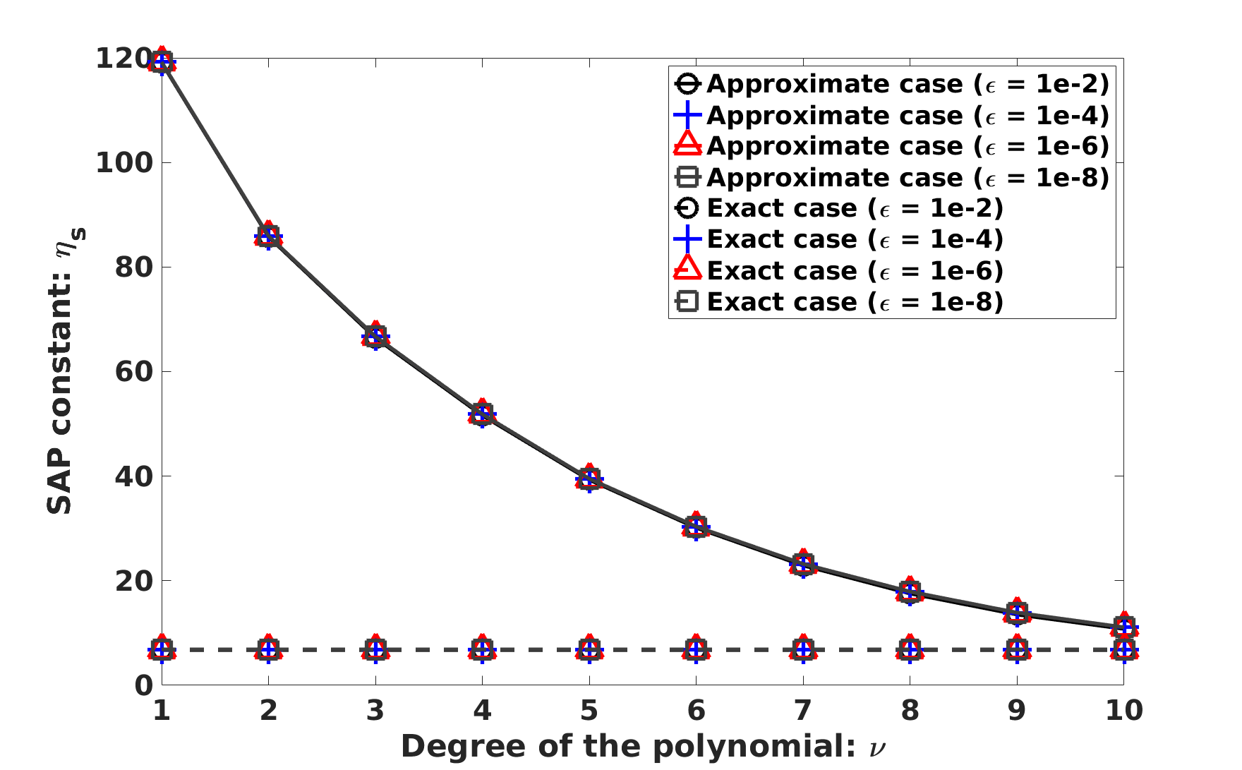
Figure 1: Example 6.1: the SAP constants for different $\epsilon$ ($h=1/64$, $N=4,225$ and $N_{c}=302$)

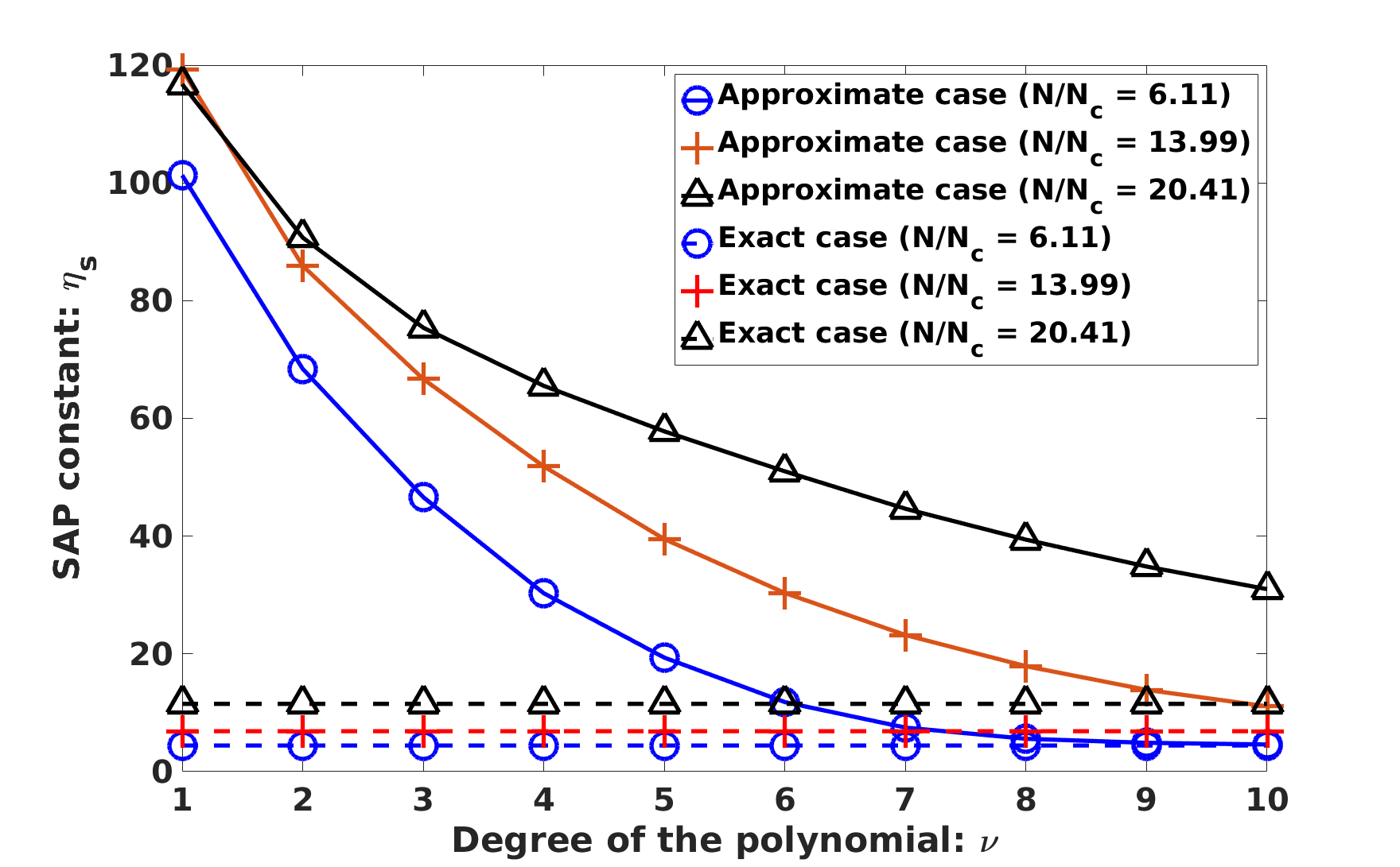
Figure 2: Example 6.1: the SAP constants for different $N_{c}$ ($h=1/64$, $N=4,225$ and $\epsilon=10^{-4}$)

The next test illustrates the properties of the coarse matrices corresponding to the modified coarse spaces based on polynomial approximation. More specifically, we are interested in the sparsity of the modified prolongation matrix ${\widetilde{P}}$ (in terms of percentage w.r.t to the matrix size $NN_{c}$). We also are interested in the AMG operator complexity (OC) defined as the ratio between the total number of nonzeros of $A$ plus the number of the nonzeros of the coarse-level matrix and the number of nonzeros of $A$. Note that $\nu=0$ corresponds to the original prolongation $P$ (and respective coarse matrix). From Table 1, as expected, we see that both the number of nonzeros and operator complexity grow when $\nu$ increases. The number of nonzeros of ${\widetilde{P}}$ grows faster when the ratio $\frac{N}{N_{c}}$ gets bigger whereas the operator complexity actually grows slower when $\frac{N}{N_{c}}$ gets larger. We note that in practice, for upscaling purposes, we need to have operator complexity less than two (then we use less memory to store the coarse matrix than the original fine-level one). Our results indicate that to achieve desired approximation accuracy for a reasonable computational cost can be a challenging task. In addition, we also use the modified coarse space in AMG iterative method and report number of iterations of the two-grid algorithms. Here, we choose $f=1$ in the diffusion problem (5.1). In the two-grid algorithm, Gauss-Seidel relaxation is used, with zero initial guess and the stopping criterion is achieving a reduction of the $\ell_{2}$ norm of the relative residual by $10^{-6}$. As expected, the number of iterations (Iter) decreases as $\nu$ increases. We note that in practice for solving linear systems, we need to consider the trade-off between the computational complexity and convergence behavior. The latter can also be a challenge in practice.

Table 1: Example 6.1: sparsity of the modified coarse space and performance of two-grid AMG method with different $\nu$ ($h=1/64$, $N=4,225$ and $\epsilon=10^{-4}$)

	$N/N_{c}=6.11$			$N/N_{c}=13.99$			$N/N_{c}=20.41$
	nnz of ${\widetilde{P}}$	OC	Iter	nnz of ${\widetilde{P}}$	OC	Iter	nnz of ${\widetilde{P}}$	OC	Iter
$\nu=0$	$0.15\%$	$1.22$	$43$	$0.43\%$	$1.13$	$52$	$1.2\%$	$1.15$	$60$
$\nu=1$	$0.92\%$	$2.19$	$30$	$2.75\%$	$1.63$	$42$	$6.97\%$	$1.65$	$55$
$\nu=2$	$2.52\%$	$3.92$	$23$	$7.27\%$	$2.41$	$38$	$17.55\%$	$2.24$	$50$
$\nu=3$	$4.92\%$	$6.62$	$19$	$13.78\%$	$3.29$	$34$	$31.35\%$	$2.73$	$48$
$\nu=4$	$8.14\%$	$8.89$	$16$	$21.87\%$	$4.10$	$30$	$45.87\%$	$2.98$	$46$
$\nu=5$	$12.07\%$	$11.71$	$14$	$30.96\%$	$4.74$	$28$	$60.04\%$	$3.10$	$41$

Example 6.2.

To stress upon the fact that our approach is in fact purely algebraic, we apply our results to graph Laplacian systems corresponding to graphs listed in Table 2.

Table 2: A set of networks from different real-world applications (first three graphs are from Stanford Large Network Dataset Collection [19] and the last graph is from SuiteSparse Matrix Collection [7]). For each graph, we show its number of vertices, number of edges, average vertex degree (ave. deg.) and maximal vertex degree (max. deg.)

	Vertices	Edges	ave. deg.	max. deg.	Description
bitcoin-alpha	3,775	14,120	7.48	510	Bitcoin Alpha web of trust network
ego-facebook	4,039	88,234	43.69	1045	Social circles from Facebook
ca-GrQc	4,158	13,425	6.46	81	Collaboration network of Arxiv
rw5151	5,151	15,248	5.92	7	Markov chain modeling

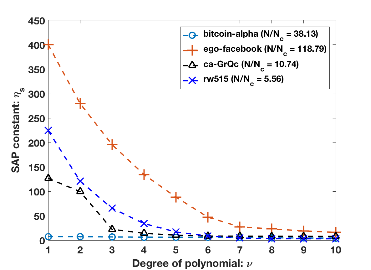
Figure 3: Example 6.2: the SAP constants for different $\nu$

In Figure 3, we present the SAP constants for the different graphs from Table 2. Here, we use a simple unsmoothed aggregation approach. In order to achieve aggressive coarsening, the aggregates are built based on the sparsity pattern of $L^{2}$, where $L$ corresponds to the graph Laplacian. The original coarse space (or respective interpolation matrix $P$) is constructed using the spectral AMGe method (as used in [12]). As we can see, although the ratio $\frac{N}{N_{c}}$ differs for the different graphs, if we use relatively accurate approximation (i.e. relatively large $\nu$), the SAP constant stays small and is fairly similar for different graphs. This demonstrate that the modified coarse spaces are also robust for these real-world graphs.

In Figure 4 and 5, we illustrate the sparsity of the modified prolongations and respective coarse matrices. We notice that the nonzeros percentage of ${\widetilde{P}}$ grows fairly quickly, which suggests that in practice, only small $\nu$ makes sense. If the coarse level problem are meant to be used multiple times, due to reasonable operator complexity and good approximation property achieved by large $\nu$, we could use more accurate approximated modified coarse spaces coming from relatively large $\nu$. For graphs with irregular degree distribution, the challenge to maintain reasonable sparsity of the coarse matrices with good approximation properties is much more pronounced than in the discretized PDE case and it requires more specialized study.

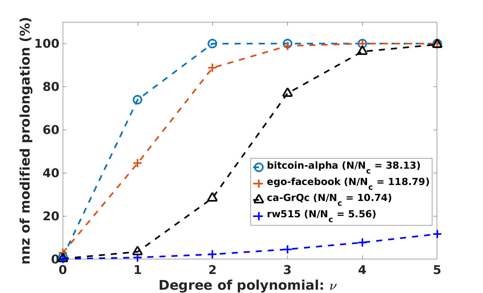
Figure 4: Example 6.2: number of nonzeros of ${\widetilde{P}}$ (in percentage) for different $\nu$

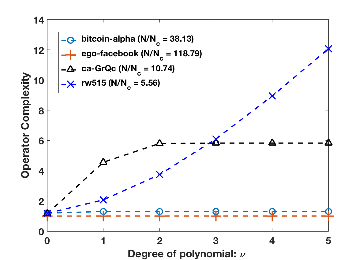
Figure 5: Example 6.2: operator complexity for different $\nu$

7 Conclusions

In this paper, we investigate the use of certain AMG coarse spaces for the purpose of dimension reduction which in the present setting is referred to as numerical upscaling. As it is well-understood that although the traditional AMG coarse spaces do satisfy the WAP (weak approximation property), it is not sufficient for the purpose of upscaling because the coarse-level solutions do not necessarily approximate the fine-level solution with guaranteed accuracy. To remedy this, we follow the approach developed in [22] extending it to the presented AMG setting. The method exploits a projection $\pi_{f}$ used to modify the original coarse space, which is assumed to possess a WAP, so that the resulting new, modified, coarse space satisfies a SAP (strong approximation property) with provable satisfactory bound on the resulting constant $\eta_{s}$. More specifically, the modified coarse space is one of the components in a two-level $A$-orthogonal decomposition so that the corresponding coarse-level solution gives accurate approximation in energy norm. One main challenge with this approach is the fact that the matrix $A_{f}^{-1}$ used in the definition of $\pi_{f}$, is dense even if $A_{f}$ is sparse. Thus, modifying the original coarse space with exact $\pi_{f}$ is computationally infeasible (for large-scale problems). In order to make such modification more practical, we use the fact (which we prove) that $A_{f}$ is well-conditioned, allowing the use of polynomials to approximate its inverse, leading to an approximate $\pi_{f}$, which is used to define an approximate modified coarse space. Such approximation is computational feasible and also provides provable error estimates in energy norm. Moreover, the error estimates improve when increasing the degree of the polynomial used in the approximation.

We provide numerical results that illustrate the theory and demonstrate the accuracy and sparsity of the coarse problems coming from the approximately modified coarse space. The tests include both, examples of diffusion equation with high contrast coefficients as well as graph Laplacian matrices corresponding to some real-life applications.

As discussed, the use of such modified coarse spaces is of interest in dimension reduction which, as our model tests demonstrate, can be challenging for the present approach (in terms of maintaining reasonable sparsity of the coarse matrices). In the PDE case this challenge seems resolvable if large enough coarsening factor ($H/h$) is employed, whereas in the graph application for graphs with irregular degree distribution, in addition to high coarsening factor one may need to employ graph disaggregation (cf., [16]), which is left for a possible future study. Additionally, in the PDE case, it is of interest to extend the present results to other types of PDEs such as ones posed in $H(\operatorname{curl})$ and $H(\operatorname{div})$, which will provide alternatives to the existing AMGe upscaling methods (cf., [17], [13], and [1]).

References

- [1] A. Barker, C. S. Lee, and P. S. Vassilevski, “Spectral Upscaling for Graph Laplacian Problems with Application to Reservoir Simulation,” SIAM Journal on Scientific Computing 39(5)(2017), pp. S323-S346.
- [2] A. Brandt, S. McCormick, and J. Ruge, ”Algbraic Multigrid (AMG) for Sparse Matrix Equations,” in Sparsity and Its Applications, Edited by David J. Evans, Cambridge University Press, Cambridge, 1985, pp. 257–284.
- [3] T. Chartier, R. Falgout, V.E. Henson, J. Jones, T. Manteuffel, S. McCormick, J. Ruge, and P.S. Vassilevski, “Spectral AMGe (AMGe),” SIAM Journal on Scientific Computing, 25(1)(2003), pp. 1-26.
- [4] M. Brezina, R. Falgout, S. MacLachlan, T. Manteuffel, S. McCormick, and J. Ruge, “Adaptive smoothed aggregation multigrid,” SIAM Rev., 47(2)(2005), pp. 317-346.
- [5] M. Brezina and P. Vassilevski, “Smoothed aggregation spectral element agglomeration AMG: AMGe,” in Large-Scale Scientific Computing, 8th International Conference, LSSC 2011, Sozopol, Bulgaria, June 6-10th, 2011. Revised Selected Papers. Lecture Notes in Computer Science, vol. 7116, Springer, 2012, pp. 3–15.
- [6] M. Brezina, P. Vaněk, and P. S. Vassilevski, “An Improved Convergence Analysis of Smoothed Aggregation Algebraic Multigrid,” Numerical Linear Algebra with Applications 19(3)(2012), pp. 441-469. (published online: 2 MAR 2011, DOI: 10.1002/nla.775).
- [7] T. A. Davis and Y. Hu, “The university of Florida sparse matrix collection,” ACM Transactions on Mathematical Software, 38(1), 2011, pp. 1-25.
- [8] P. D’Ambra and P. S. Vassilevski, “Adaptive AMG with Coarsening Based on Compatible Weighted Matching,” Computing and Visualization in Science 16 (2013), pp. 59-76.
- [9] S. Demko, W.F. Moss, and P.W. Smith, ”Decay rates of inverses of band matrices”, Mathematics of Computation 43(168)(1984), pp. 491-499.
- [10] R. Falgout, P. S. Vassilevski, and L. T. Zikatanov, “On Two-grid Convergence Estimates,” Numerical Linear Algebra with Applications, 12(5-6), 2005, pp. 471-494.
- [11] T. Grauschopf, M. Griebel, and H. Regler, “Additive multilevel preconditioners based on bilinear interpolation, matrix-dependent geometric coarsening and algebraic multigrid coarsening for second-order elliptic PDEs,” Applied Numerical Mathematics, Multilevel Methods 23, 1997, pp. 63–95
- [12] X. Hu, P. S. Vassilevski, and J. Xu, “A two-grid SA-AMG convergence bound that improves when increasing the polynomial degree,” Numerical Linear Algebra with Applications 23(4)(2016), pp. 746–771.
- [13] D. Kalchev, C. S. Lee, U. Villa, Y. Efendiev, and P. S. Vassilevski, Upscaling of Mixed Finite Element Discretization Problems by the Spectral AMGe Method, SIAM Journal on Scientific Computing 38(5) (2016), pp. A2912-A2933.
- [14] T. V. Kolev and P. S. Vassilevski, “Parallel auxiliary space AMG for H(curl) problems,” Journal of Computational Mathematics 27(2009), pp. 604–623.
- [15] T. V. Kolev and P. S. Vassilevski, “Parallel auxiliary space AMG for H(div) problems,”S SIAM Journal on Scientific Computing 34(2012), pp. A3079-A3098.
- [16] V. Kuhlemann and P. S. Vassilevski, “Improving the Communication Pattern in Mat-Vec Operations for Large Scale-free Graphs by Disaggregation,” SIAM Journal on Scientific Computing 35(5)(2013), pp. S465-S486.
- [17] I. V. Lashuk and P. S. Vassilevski, “The Construction of Coarse de Rham Complexes with Improved Approximation Properties,” Computational Methods in Applied Mathematics 14(2)(2014), pp. 257-303.
- [18] J.V. Lent, R. Scheichl, I.G. Graham, “Energy-minimizing coarse spaces for two-level Schwarz methods for multiscale PDEs,” Numerical Linear Algebra with Applications 16, 2009, pp. 775–799.
- [19] J. Leskovec and A. Krevl, “SNAP Datasets: Stanford Large Network Dataset Collection, http://snap.stanford.edu/data.
- [20] Oren E. Livne and Achi Brandt, “Lean Algebraic Multigrid (LAMG): Fast Graph Laplacian Linear Solver,” SIAM Journal on Scientific Computing 34(4) (2012), pp. B499-B522
- [21] S.P. MacLachlan and J.D. Moulton, “Multilevel upscaling through variational coarsening,” Water Resources Research 42, 2006.
- [22] A. Malqvist and D. Peterseim, “Localization of elliptic multiscale problems,” Math. Comp., 83(290), pp. 2583-2603, 2014.
- [23] J.D. Moulton, J.E. Dendy, and J.M. Hyman, “The Black Box Multigrid Numerical Homogenization Algorithm.,” Journal of Computational Physics 142, 1998, pp. 80–108.
- [24] S. Reitzinger and J. Schöberl, “An algebraic multigrid method for finite element discretizations with edge elements,” Numerical Linear Algebra with Applications 9(3) (2002), pp. 223-238.
- [25] P. S. Vassilevski, “On two ways of stabilizing the HB multilevel methods,” SIAM Review 39(1997), 18–53.
- [26] N. Spillane, V. Dolean, P. Hauret, F. Nataf, C. Pechstein, and R. Scheichl, “Abstract robust coarse spaces for systems of PDEs via generalized eigenproblems in the overlaps,” Numer. Math. 126, 2014, pp. 741–770.
- [27] Panayot S. Vassilevski, “Coarse Spaces by Algebraic Multigrid: Multigrid Convergence and Upscaling Error Estimates,” Advances in Adaptive Data Analysis, 3(1&2), pp. 229-249, 2011.
- [28] Panayot S. Vassilevski, “Multilevel Block Factorization Preconditioners, Matrix-based Analysis and Algorithms for Solving Finite Element Equations,” Springer, New York, 2008. 514 p.
- [29] Jinchao Xu and Ludmil Zikatanov, “Algebraic multigrid methods,” Acta Numerica 26(2017), pp. 591-721.