A Survey of Nuclear Pasta in the Intermediate Density Regime
I: Shapes and Energies

Abstract

Background

Nuclear pasta, emerging due to the competition between the long-range Coulomb force and the short-range strong force, is believed to be present in astrophysical scenarios, such as neutron stars and core-collapse supernovae. Its structure can have a high impact e.g. on neutrino transport or the tidal deformability of neutron stars.

Purpose

We study several possible pasta configurations, all of them minimal surface configurations, which are expected to appear in the mid-density regime of nuclear pasta, i.e. around 40% of the nuclear saturation density. In particular we are interested in the energy spectrum for different pasta configurations considered.

Method

Employing the density functional theory (DFT) approach, we calculate the binding energy of the different configurations for three values of the proton content $X_{P}=1/10,\,1/3$ and $1/2$, by optimizing their periodic length. We study finite temperature effects and the impact of electron screening.

Results

Nuclear pasta lowers the energy significantly compared to uniform matter, especially for $X_{P}\geq 1/3$. However, the different configurations have very similar binding energies. For large proton content, $X_{P}\gtrsim 1/3$, the pasta configurations are very stable, for lower proton content temperatures of a few MeV are enough for the transition to uniform matter. Electron screening has a small influence on the binding energy of nuclear pasta, but increases its periodic length.

Conclusion

Nuclear pasta in the mid-density regime lowers the energy of the matter for all proton fractions under study. It can survive even large temperatures of several MeV. Since various configurations have very similar energy, it is to expect that many configurations can coexist simultaneously already at small temperatures.

I Introduction

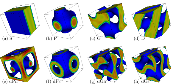
Figure 1: One cubic elementary cell for all studied pasta configurations with $X_{P}=0.5$ and a mean density of $\rho=0.05\mathrm{\,fm}^{-3}$. Slab (a), P-surface (b), Gyroid (c), Diamond (d), network-like double P-surface (e), surface-like double P-surface (f), network-like double Gyroid (g), surface-like double Gyroid (h). The color scale is in units of $\mathrm{\,fm}^{-3}$.

The recent observation of gravitational waves from the neutron star merger event GW170817 Abbott et al. (2017) and its electromagnetic transient (AT 2017gfo) Abbott et al. (2017), which identifies neutron star mergers as a site for the r process, has opened new avenues to study the physics of matter in neutron stars Tews et al. (2019); Gandolfi et al. (2019). Gravitational wave observations have been used to determine the tidal polarizability (or deformability) of neutron stars and hence put limits on the stellar radii and the underlying equation of state De et al. (2018a); *De.Finstad.ea:2018err; Abbott et al. (2018). In addition to stellar compactness, the tidal polarizability is sensitive to the second tidal Love number that has been shown to depend on the inner crust of the neutron star Piekarewicz and Fattoyev (2019).

The properties of the inner crust of neutron stars are affected by the presence of nuclear pasta matter. Pasta matter is named for its resemblance to Italian pasta, e.g. spaghetti and lasagna Ravenhall et al. (1983); Hashimoto et al. (1984) and is formed because of the competition between the long-range Coulomb force and the short range nuclear force (Coulomb frustration). It can appear at densities between about 10% and 90% percent of the nuclear saturation density and low enough temperatures. It is not possible to create an environment for nuclear pasta in the laboratory. However, first effects of Coulomb frustration can be observed in superheavy nuclei Davies et al. (1972); Wong (1973); Dietrich and Pomorski (1998); Dechargé et al. (1999); Schuetrumpf et al. (2017); Staszczak et al. (2017).

A second site for nuclear pasta matter are core-collapse supernovae. While in neutron stars the proton content of the nuclear matter in the inner crust is expected to be about $X_{P}=1/10$ and temperatures are low, the proton fraction in supernovae can be much higher and temperatures can reach up to about 40 MeV. Nuclear pasta matter can have a strong influence on the neutrino transport Horowitz et al. (2004a, b); Sonoda et al. (2007); Grygorov et al. (2010); Roggero et al. (2018). Due to its location in the neutron star, nuclear pasta can leave an imprint on the neutrino spectrum of neutron stars. Furthermore, elastic properties of nuclear pasta are different from uniform matter or from spherical nuclei Caplan et al. (2018).

Nuclear pasta has been studied with various approaches. Beside classical theories, such as the liquid drop model and (quantum) molecular dynamics calculations Dorso et al. (2012); Caplan et al. (2018) with which it is possible to include vast numbers of nucleons and to simulate very large systems, quantum theories, e.g. the Thomas-Fermi theory Williams and Koonin (1985); Okamoto et al. (2013); Pais et al. (2015) and density functional theory (DFT) Bonche and Vautherin (1981); Magierski and Heenen (2002); Gögelein and Müther (2007); Newton and Stone (2009); Pais and Stone (2012); Schuetrumpf et al. (2013, 2014, 2015); Schuetrumpf and Nazarewicz (2015); Fattoyev et al. (2017), have also been employed. In these studies, it has been discovered that not only the basic pasta structures such as the rod (spaghetti) or the slab (lasagna) and their reversed (bubble) configurations can be realized, but also much more complicated configurations. Among them is the parking ramp configuration Berry et al. (2016), similar to a slab configuration but with defects, the Gyroid and the Diamond Schuetrumpf et al. (2015); Nakazato et al. (2009, 2011), and the P-surface configurations Schuetrumpf et al. (2013) (see Fig. 1). The latter three are triply periodic minimal surfaces (TPMS) and connect the research of nuclear pasta to different fields, e.g., solid biological systems Michielsen and Stavenga (2008); Schröder-Turk et al. (2011), di-block copolymers Hajduk et al. (1994) and lipid-water systems Larsson (1989).

In this work, we aim to give a comprehensive picture on pasta configurations which are expected to form at the intermediate density regime, $\rho\lesssim\rho_{0}/2$, including the TMPS, with the DFT approach. In Sec. II, we introduce our DFT implementation, as well as TPMS and the method to extract observables from the calculations. In Sec. III, we study the configurations at zero temperature, in Sec. IV we introduce finite temperature and in Sec. V we estimate the impact of electron screening. Finally, we give details of the computational aspects in Sec VI.

II Method

II.1 The DFT approach

In this work, the tool of choice to examine pasta configurations is the DFT approach Bender et al. (2003). We consider DFT at the Hartree-Fock (HF) level, i.e., without pairing correlations which would be accounted for by HF+BCS or full Hartree-Fock-Bogolyubov (HFB) calculations. However they are not computationally feasible for the large systems considered here. The DFT method can predict many features, e.g., nuclear masses, radii or deformations of nuclei all across the nuclear chart, and is therefore a valid tool also for nuclear pasta.

We choose a standard Skyrme type parametrization of the DFT functional. In particular, we choose the TOV-min parametrization Erler et al. (2013) and use it throughout this work. This interaction is not only fitted to stable nuclei and infinite matter properties, but also to reproduce the mass-radius relation for neutron stars which makes it very relevant for this work.

As engine to solve the DFT problem, we use the code Sky3D Maruhn et al. (2014); Schuetrumpf et al. (2018). It operates on a 3D equidistant grid in a rectangular computational box. The derivatives are performed utilizing the Fast Fourier Transform (FFT) technique which makes it easy to implement periodic boundary conditions (PBC) for our pasta calculations. We assume periodic systems to overcome the mismatch in size between the quantum system feasible to simulate on a supercomputer involving a few thousand nucleons Afibuzzaman et al. (2018) and the macrocopic length scale of a few hundred meters of the inner crust of a neutron star. However, it has been shown that strict PBC for the wave functions lead to spurious finite-volume effects Schuetrumpf and Nazarewicz (2015). To reduce those errors, we employ the twist-averaged boundary conditions (TABC) Schuetrumpf and Nazarewicz (2015). We use TABC for zero-temperature calculations with a cubic box length of $L\lesssim 24\mathrm{\,fm}$. For finite-temperature and large box lengths, we have checked that PBC are sufficient due to the large number of single-particle momentum states that are (partly) occupied.

II.1.1 Finite temperature

For finite-temperature calculations, we allow the states to be partly occupied. The density can be obtained by

$$\rho_{q}(\mbox{\boldmath$r$})=\sum_{\alpha}f_{\alpha,q}|\psi_{\alpha,q}(\mbox{\boldmath$r$})|^{2}$$ (1)

where $q$ denotes the isospin (neutron or proton) and $\alpha$ the HF single-particle state, $f_{\alpha,q}$ is the Fermi distribution for neutrons and protons separately. Chemical potentials are determined from the particle number constraint. The sum over HF single-particle states is such that for the highest state in energy $f_{\alpha,q}<0.01$. Instead of minimizing the internal energy of the system, for finite-temperature calculations the HF technique minimizes the free energy $F=E-TS$. The entropy of the system can be obtained from

$$S=-\sum_{\alpha,q}\left[f_{\alpha,q}\ln(f_{\alpha,q})+(1-f_{\alpha,q})\ln(1-f_{\alpha,q})\right]\quad.$$ (2)

II.1.2 Electron screening

In Sec. V, we will estimate the effect of a non-uniform electron distribution on nuclear pasta. Electrons will be attracted by the positive charge distribution coming from the protons and effectively screen the Coulomb potential from the protons.

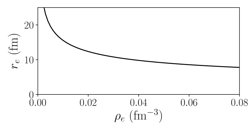
Figure 2: Electron screening radius as a function of mean electron density.

To account for electron screening we use the Thomas-Fermi approximation that leads to the Poisson equation Haensel et al. (2007)

$$\left(\mbox{\boldmath$\nabla$}^{2}+k^{2}_{\rm TF}\right)\phi(\mbox{\boldmath$r$})=-4\pi\rho_{p}(\mbox{\boldmath$r$})\quad,$$ (3)

taking the charge distribution as the proton distribution $\rho_{p}$. It can easily be solved in Fourier space

$$\tilde{\phi}(\mbox{\boldmath$k$})=\frac{-4\pi\tilde{\rho}_{p}(\mbox{\boldmath$k$})}{(-\mbox{\boldmath$k$}^{2}+k^{2}_{\rm TF})}\quad.$$ (4)

The Thomas-Fermi wave number is

$$k_{\rm TF}=r_{e}^{-1}=\left(4\pi e^{2}\frac{\partial\rho_{e}}{\partial\mu_{e}}\right)^{1/2}$$ (5)

and its inverse, $r_{e}$, the electron screening length. For a strongly degenerate electron gas, which we consider here in this work, the Thomas-Fermi wave number can be expressed as Haensel et al. (2007)

$$k_{\text{TF}}=2\sqrt{\frac{\alpha_{f}\sqrt{1+x_{r}^{2}}}{\pi x_{r}}}k_{\mathrm{F}}$$ (6)

where $x_{r}=\hbar k_{\mathrm{F}}/(m_{e}c)$, $\alpha_{f}$ is the fine structure constant and $k_{\mathrm{F}}=(3\pi^{2}\rho_{e})^{1/3}$ is the Fermi momentum of the electrons. The mean electron density, $\rho_{e}$, due to charge neutrality is the same as the mean proton density. The resulting electron screening length as a function of the mean electron density is shown in Fig. 2.

II.2 Minimal Surfaces for Nuclear Pasta

The goal of this work is to determine the binding energy of nuclear pasta in the intermediate density regime where the configurations shown in Fig. 1 are expected to appear. To that end, we have to find the optimal pasta configuration for a given mean density, proton fraction and temperature. Generally, all possible configurations have to be assumed and from those the one with minimal energy is considered as the ground state. In this work, we only consider the periodic configurations shown in Fig  1. The simplest among them is the slab (S) configuration which has already been studied from the very beginning of pasta matter research. The others we consider are the Schwarz Primitive (P-)surface, Diamond (D-)surface, and Gyroid (G-)surface. Their nodal approximations are

$$\phi_{S} =\cos X$$ (7a)

$$\phi_{P} =\cos X+\cos Y+\cos Z$$ (7b)

$$\phi_{G} =\cos X\sin Y+\cos Y\sin Z+\cos Z\sin X$$ (7c)

$$\phi_{D} =\cos X\cos Y\cos Z+\cos X\sin Y\sin Z$$

$$+\sin X\cos Y\cos Z+\sin X\sin Y\cos Z\quad,$$ (7d)

where $X=2\pi x/L$ and likewise for the other directions.

In first order, the minimal surfaces can be parametrized with the nodal approximations as $\phi_{i}=0$ with $i\in\{S,P,G,D\}$. The surface divides the space into two completely separated half spaces with equal volume and equal topology. Only the Gyroid divides the space into two half spaces with opposite chirality. When the half spaces are not divided equally, we can approximate the surface as $\phi_{i}=t$ for small values of $t$. If one half space or domain is filled with nuclear matter and the other is empty or only filled with a neutron background gas, we call those configurations “single” configurations. “Double” configurations are enclosed by two surfaces $\phi_{i}=\pm t$. For double configurations there are two possibilities: Either the surface-like domain $|\phi_{i}|<t$ or the network-like domain $|\phi_{i}|>t$ can be filled with nuclear matter. Henceforth, they are labeled as e.g. dGs for double Gyroid surface-like and similar for the other double configurations. We do not consider the double Diamond configurations, because their preferred periodic lengths are too large and computationally not feasible.

	S	P	G	D
$\chi$	0	-2	-4	-8
$A_{1}$	2.0	2.15652	2.65624	3.3715

Table 1: Euler characteristic $\chi$ per cubic unit cell and surface area $A_{1}$ for an assumed box length of 1 for single minimal surface configurations.

The TPMS (P, G, and D) are related to each other by the Bonnet transformation, which transforms the shapes smoothly into each other Hyde et al. (1997). Our three candidates are the only physically relevant surfaces, since all others are self-intersecting. A difference between the surfaces is that they have different surface areas for the same periodic length

$$A_{i}=A_{1,i}\times L^{2},\quad i\in\{S,P,G,D\}.$$ (8)

The configurations also have different Euler characteristics for one cubic unit cell, which is often used to discriminate pasta configurations. It is defined as

$$\chi=\#(\text{connected components})-\#(\text{holes})+\#(\text{cavities})$$ (9)

The values for $A_{1,i}$ and $\chi$ for a cubic elementary cell are given in Table 1 Schröder et al. (2003).

II.3 Minimizing the pasta binding energy

For each configuration, we perform DFT calculations for a fixed average density and proton fraction in a given computational box which is equal to the periodic length of the configuration. By varying the periodic length, we determine the energy of each configuration as a function of periodic length. The binding energy corresponds to the energy minimum that in general is obtained at different optimal periodic lengths for each configuration.

In order to computationally define a certain configuration, we fix the mean-field for the first 200 iterations of the DFT calculations. For the single configurations we take a guiding potential of the form of the nodal approximations, i.e.

$$U_{{\rm single,\,}it<200}=\phi_{0}\cdot\phi_{i},\quad i\in\{S,P,G,D\},$$ (10)

where $\phi_{0}$ is a constant optimized to speed up convergence. Consequently, the matter will arrange itself in the domain, where $\phi_{i}(\mbox{\boldmath$r$})<0$.

For the double configurations, we take the guiding potential of the form

$$U_{{\rm double,\,}it<200}=\pm\phi_{0}\cdot|\phi_{i}|,\quad i\in\{P,G\},$$ (11)

where the positive sign leads to the surface-like configuration and the negative sign leads to the network-like configuration.

After 200 iterations, we perform standard DFT calculations at the HF level with the self-consistent potential and find the local minimum. Eventually, calculations yield the desired configuration. If the actual box length is far off the optimal length, the configuration can be unstable and will then be transformed into some other configuration. Those cases are not considered.

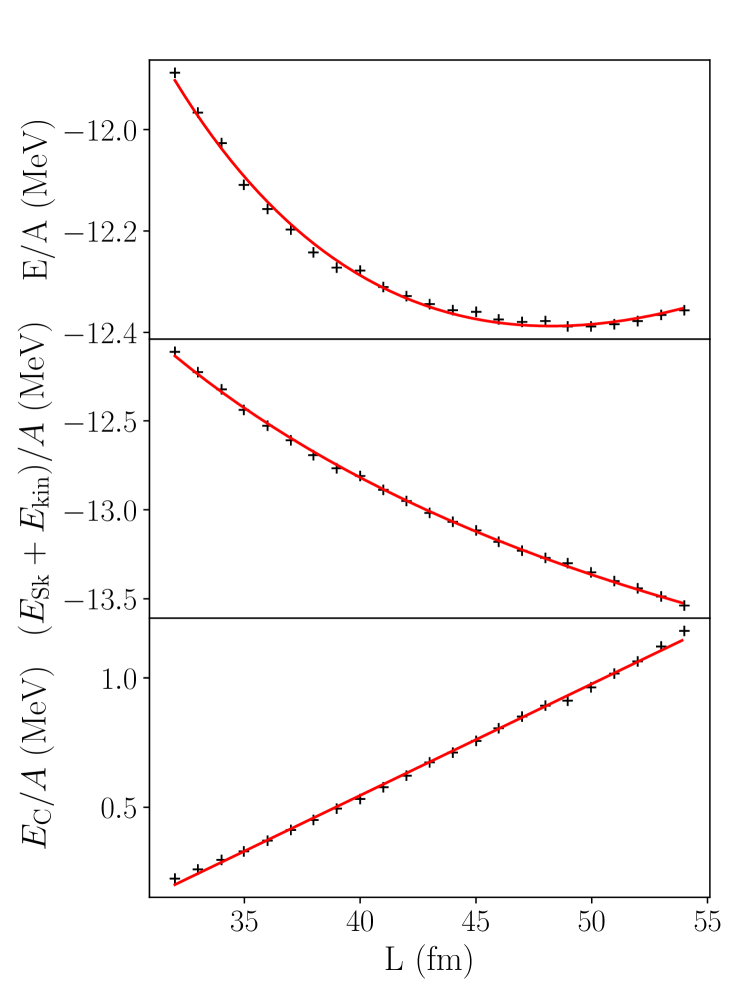
Figure 3: Total energy per nucleon, Skyrme energy and kinetic energy per nucleon, and Coulomb energy per nucleon as a function of the cubic periodic length $L$ for the dGs configuration with $X_{P}=0.5$ and $\rho=0.05\mathrm{\,fm}^{-3}$. The black + signs correspond to the HF calculations, the red line displays the fit to the calculations.

In order to determine the binding energy and optimal periodic length we fit the energy as a function of periodic length for the discrete computed values using a functional form based on the following assumptions. We divide the total energy into two parts: Skyrme (potential) energy plus kinetic energy and Coulomb energy containing both the direct and exchange contributions. As a function of the periodic length, Coulomb energy per particle behaves approximately linearly in the region around the optimal periodic length of the configuration. We base this assumption on empirical observation. In a liquid drop picture, the energy per particle contains two leading terms: a volume term that is constant and a surface term that behaves like $\sim L^{-1}$. In summary, we fit the parts with

$$(E/A)_{\mathrm{fit}} =aL + bL^{-1} +c$$ (12a)

$$((E_{\mathrm{Sk}}+E_{\mathrm{kin}})/A)_{\mathrm{fit}} = bL^{-1} +d$$ (12b)

$$(E_{C}/A)_{\mathrm{fit}} =aL +e,$$ (12c)

where $c=d+e$. An example for the dGs configuration is shown in Fig. 3. We determine the parameters $a,b$, and $c$ by directly fitting the total energy. Once they are known, the optimal periodic length and minimum energy are determined from the expressions: $L_{\mathrm{opt}}=\sqrt{b/a}$, $(E/A)_{\mathrm{opt}}=2\sqrt{ab}+c$.

For the production runs, we perform only 5 to 7 calculations around the optimal box length in steps of $\Delta L=2\mathrm{\,fm}$ for the shapes with smaller periodic length and $\Delta L=4\mathrm{\,fm}$ for the shapes with larger periodic length. We have estimated that this procedure gives lengths with an error of about $1\mathrm{\,fm}$ and energies with an error below $0.01\mathrm{\,MeV}$.

III Zero Temperature Pasta Matter

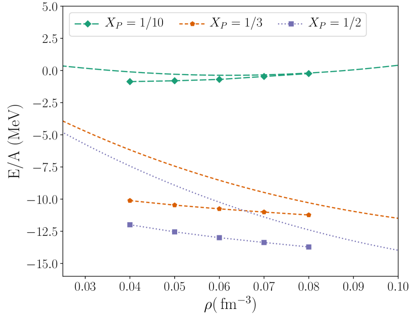
Figure 4: Comparison of total energies per nucleon of uniform matter (dashed lines) and slab (S) configuration (dashed lines with symbols) in the intermediate density regime for different proton fractions.

We consider the pasta configurations shown in Fig. 1 in the density region between $0.04\mathrm{\,fm}^{-3}$ and $0.08\mathrm{\,fm}^{-3}$ in steps of $0.01\mathrm{\,fm}^{-3}$. They are calculated for three different values for the proton content: $X_{P}\in\{1/10,1/3,1/2\}$. Depending on the computational box and mean density, the calculations involve between a few hundred up to several thousand nucleons. The computational cost is briefly discussed in Sec.VI.

Fig. 4 compares the ground state energies of the slab (S) configuration with optimal periodic length to uniform matter. For $X_{P}=1/2$ and $1/3$ at low densities the S pasta configuration is lower in energy for as much as $5\mathrm{\,MeV}$ per particle. At the highest densities studied ($0.08\mathrm{\,fm}^{-3}$) the difference is about $1\mathrm{\,MeV}$. For $X_{P}=1/10$ the energy for low densities is lowered by about $1\mathrm{\,MeV}$ and approaches the uniform matter total energy per particle for $0.08\mathrm{\,fm}^{-3}$.

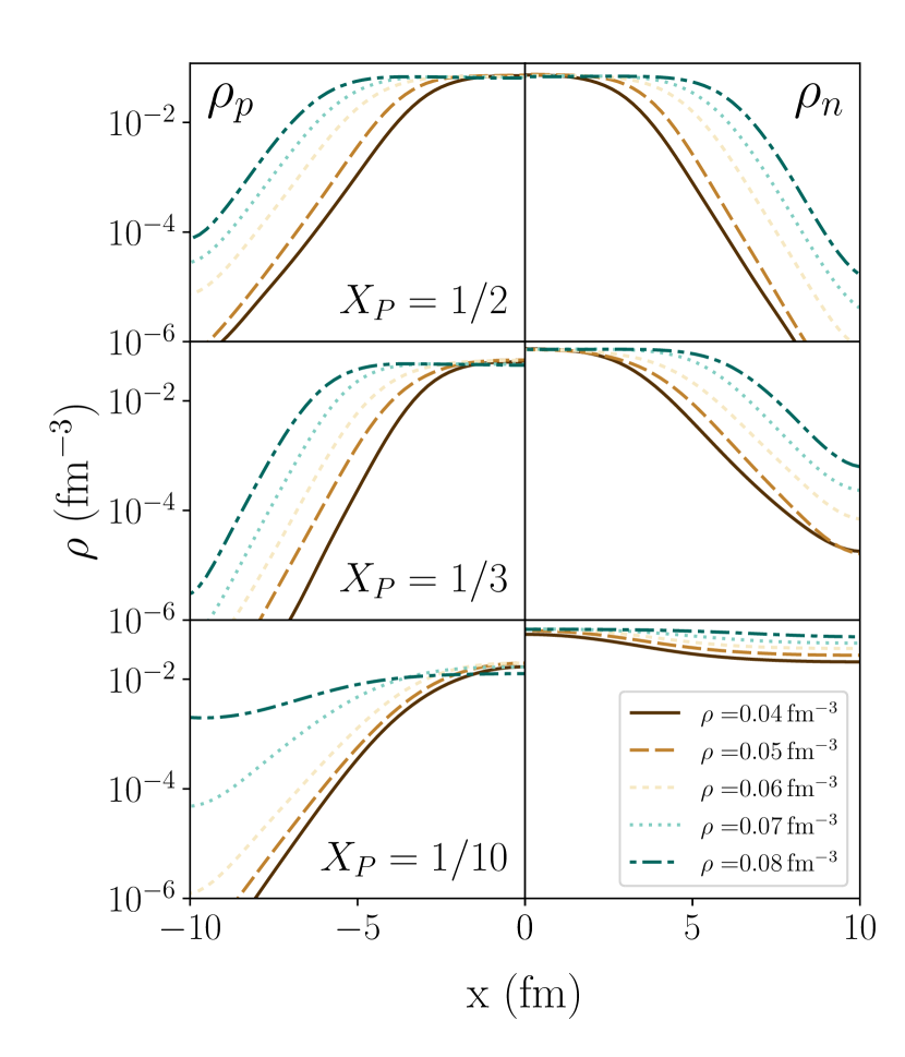
Figure 5: Density profiles for the slab configuration in the non-uniform direction. Proton densities are on the left, neutron densities are on the right panels. Symmetric nuclear matter is in the upper panel, $X_{P}=1/3$ in the mid panels and $X_{P}=1/10$ in the lower panels.

Slab density profiles for all studied mean densities and proton fractions are shown in Fig. 5. These calculations were done for a fixed periodic length of $L=20\mathrm{\,fm}$. For symmetric nuclear matter the profiles for neutrons and protons look similar. The protons have a slightly larger background density in the low density region (or void) between the slabs than the neutrons due to Coulomb repulsion. For larger mean densities the slabs extend more and the void region becomes smaller. Therefore the minimum density in the void region becomes larger, up to $10^{-4}\mathrm{\,fm}^{-3}$ for protons for a mean density of $0.08\mathrm{\,fm}^{-3}$.

For the other proton fractions considered, the maximum density inside the slab is much larger for neutrons than for protons similar to what is found in finite nuclei Schuetrumpf et al. (2017). While the proton densities become very low in the void region ($10^{-6}\mathrm{\,fm}^{-3}$ and below), some neutrons are evaporated and an appreciable neutron background is visible for $X_{P}=1/3$. For $X_{P}=1/10$ the transition to uniform matter is visible with increasing density, explaining the convergence of the energies to the uniform matter limit in Fig. 4. For the lowest densities the slab shape is still clearly visible in the proton densities.

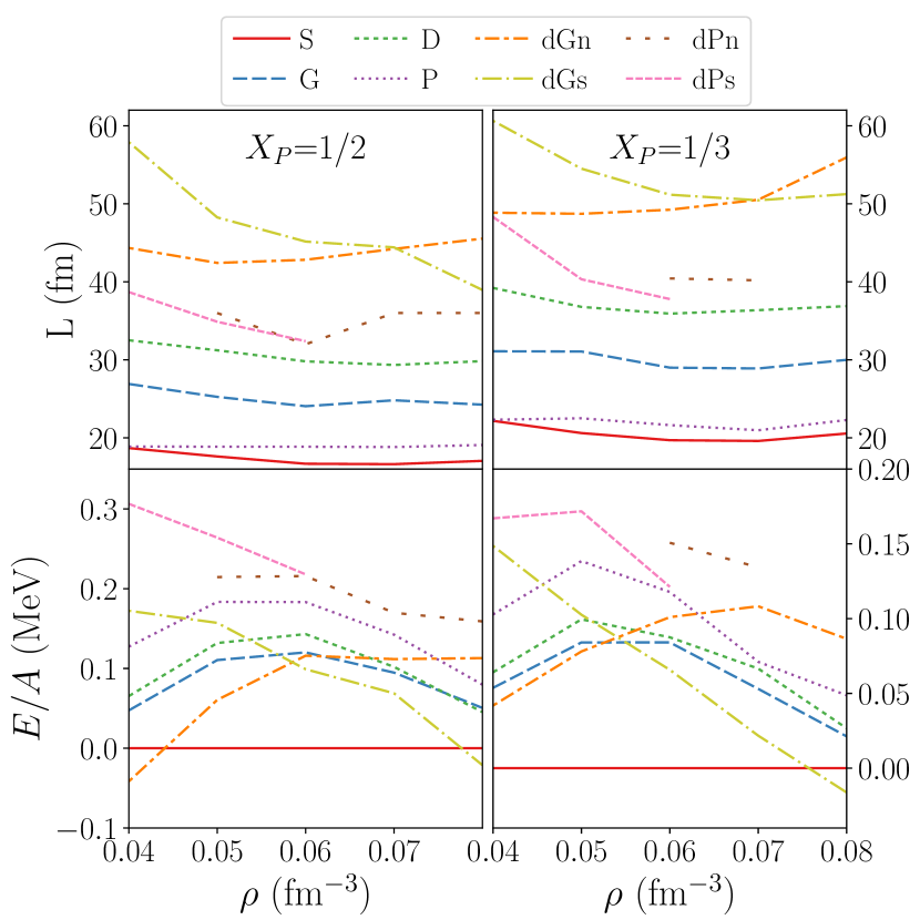
Figure 6: Optimal periodic lengths (top panels) and binding energies per particle shifted with respect to the slab shape (bottom panels) for minimal surface configurations. Left panels: $X_{P}=1/2$, right panels: $X_{P}=1/3$.

Fig. 6 shows the optimal periodic lengths and the corresponding binding energies with respect to the binding energy of the slab configuration. It has to be mentioned that for both double P topologies, stable configurations could only be obtained for a limited mean density range. The surface-like structure was stable for low densities and the network-like structure was stable for higher energies, except for $X_{P}=1/3$ and $\rho=0.08\mathrm{\,fm}^{-3}$. The unstable configurations (not shown in Fig. 6) were transformed mostly to nuclei arranged in a bcc lattice at lower densities and to nuclear bubbles at higher densities. For very large box lengths, the dPn configuration formed extra cavities at the knots, which can slightly be seen already in Fig. 1, panel (e), where yellow lower density regions appear at the corners of the box. Those shapes were not considered, as they are topologically different and out of scope of this work.

We only show the results for $X_{P}=1/2$ and 1/3. For $X_{P}=1/10$, the binding energies barely depends on the periodic length. For all the configurations the binding energy is very close to the one of the slab, especially at high mean densities. For $X_{P}\gtrsim 1/3$ none of the binding energies differ more than $0.3\mathrm{\,MeV}/A$ from the one of the slab configuration, most of them differ not more than $0.1\mathrm{\,MeV}/A$. The slab is, for most of the density range, the configuration with the lowest energy. Only for $\rho=0.4\mathrm{\,fm}^{-3}$ and $\rho=0.8\mathrm{\,fm}^{-3}$ the double gyroids, dGn or dGs, have lower energy. However at those densities different shapes come into play Schuetrumpf et al. (2013), such as the rod, anti-rod or waffle configurations, which are not discussed in this work.

$X_{P}$	1/2				1/3
shape	S	P	G	D	S	P	G	D
$\bar{L}$	$17.33$	$18.91$	$25.06$	$30.54$	$20.53$	$21.94$	$30.01$	$37.04$
$A/V$	$1.16$	$1.14$	$1.06$	$1.1$	$0.97$	$0.98$	$0.89$	$0.91$
$\chi/V$	$0$	$2.96$	$2.54$	$2.81$	$0$	$1.89$	$1.48$	$1.57$

Table 2: Optimal box length, averaged over all densities $\bar{L}$ in $\mathrm{\,fm}$, ratio of surface to volume $A/V$ in $10^{-1}\mathrm{\,fm}^{-1}$ and Euler characteristic per volume in $10^{-4}\mathrm{\,fm}^{-3}$. The surface area $A$ is estimated with Eq. (8) using $\bar{L}$ and parameters in Table 1. Volume $V$ is the unit cell box volume $V=\bar{L}^{3}$.

The optimal periodic lengths of the single shapes (S,P,G,D) are almost constant in the range of mean densities under study. It is interesting to note that the ratio of surface to volume is almost constant for all four singe shapes (see Table 2). This results also in an almost equal Euler characteristic per volume, except for the slab shape, where the Euler characteristic is always zero. In contrast, the optimal periodic lengths for surface-like double structures decrease with increasing mean density and for the network-like shapes we observe the opposite behaviour. The optimal periodic lengths for double configurations are significantly larger than those for the single configurations.

The single TPMS configurations show parabolic behavior w.r.t. the slab configuration. The maximum is around $0.06\mathrm{\,fm}^{-3}$ for $X_{P}=1/2$ and slightly shifted to lower densities for $X_{P}=1/3$. The energy per particle is decreasing for surface-like configurations with increasing mean density and tendentiously increasing for network-like configurations. While the double gyroid has lower energy than all of the single TPMS configurations (the network-like structure for lower energies and surface-like for higher energies), the double P configurations are both higher in energy.

IV Finite Temperature

In this section, we study the impact of temperature on pasta shapes. As a representative configuration, we chose the slab configuration because it is the most bound or ground state configuration. Thus, the temperature at which the slab melts represents the disappearance of the pasta phases. We restrict our investigation to the lowest mean density considered in section III, $\rho=0.04\mathrm{\,fm}^{-3}$. At this density, we find the largest difference in binding energy between pasta phases and uniform matter (see Fig. 4) and hence the largest pasta phase melting temperature.

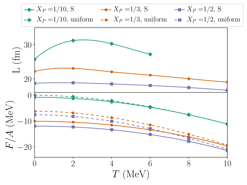
Figure 7: Optimal box length (top) and free energy of the slab at a mean density of $0.04\mathrm{\,fm}^{-3}$ with respect to temperature. The free energy is compare to the free energy of uniform matter (dashed lines). The connecting lines are simply cubic spline interpolations.

Figure 7 illustrates the optimal periodic lengths and free energy per nucleon for temperatures up to $10\mathrm{\,MeV}$. It is interesting to see that the preferred box length increases for a temperature of $2\mathrm{\,MeV}$ and then decreases for higher temperatures for all choices of $X_{P}$. For $X_{P}=1/10$ and $T\geq 8\mathrm{\,MeV}$, the density distribution becomes very close to uniform matter and therefore the optimal box length is not shown anymore.

While for zero temperature the internal or free energy for the slab and uniform matter differs by about $4.4\mathrm{\,MeV}$ for $X_{P}=1/2$ and $3.9\mathrm{\,MeV}$ for $X_{P}=1/3$, the difference for $X_{P}=1/10$ is only about $0.8\mathrm{\,MeV}$. At $T=10\mathrm{\,MeV}$, the difference shrinks to $0.5\mathrm{\,MeV}$ for $X_{P}=1/2$ and $0.35\mathrm{\,MeV}$ for $X_{P}=1/3$ and for $X_{P}=1/10$ the transition to uniform matter has already occurred between $T=6\mathrm{\,MeV}$ and $T=8\mathrm{\,MeV}$.

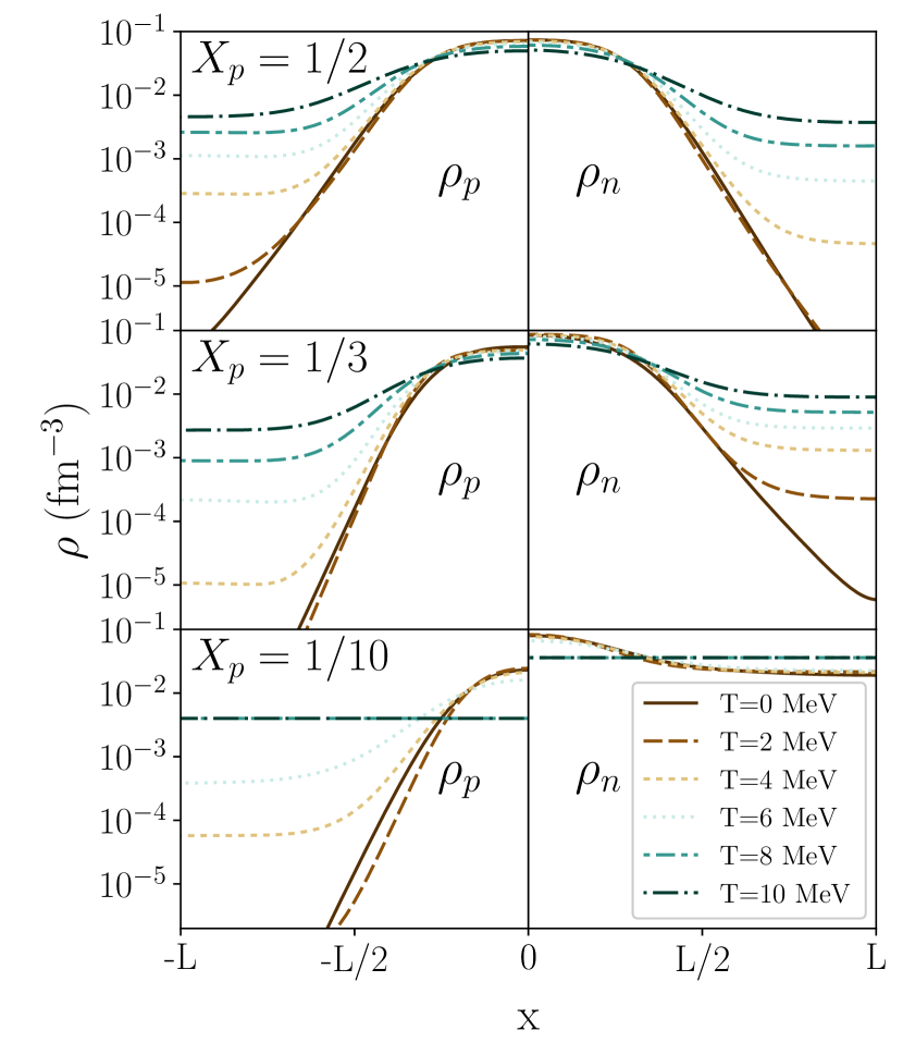
Figure 8: Density profiles for slabs at a mean density of $0.04\mathrm{\,fm}^{-3}$ with $X_{P}=1/2$ (top), $X_{P}=1/3$ (middle), $X_{P}=1/10$ (bottom) and varying temperature. Proton density is shown on the left, neutron density on the right.

In Fig. 8, the density profiles for the slabs for all investigated proton fractions and temperatures are shown. Note that the spatial direction is scaled according to the optimal box lengths to fit into the same plot. It is interesting to note that while increasing the temperature to $T=2\mathrm{\,MeV}$, the fraction of the surface area between the nuclear matter phase and the void or background phase becomes smaller. Going to higher temperatures, the transition is much more smooth and the surface area increases. At $T=10\mathrm{\,MeV}$, the densities of the $X_{P}=1/2$ and $1/3$ slabs are still clearly distinguishable from uniform matter. The transition takes place at still higher temperatures.

V Electron Screening

In the previous sections, we assumed that electrons form a uniform background. However, electrons in this very dense environment can have an influence and gather in the areas with high proton charge density. Thus the electrons partly shield the Coulomb potential from the protons and reduce the Coulomb energy. This phenomenon is called electron screening.

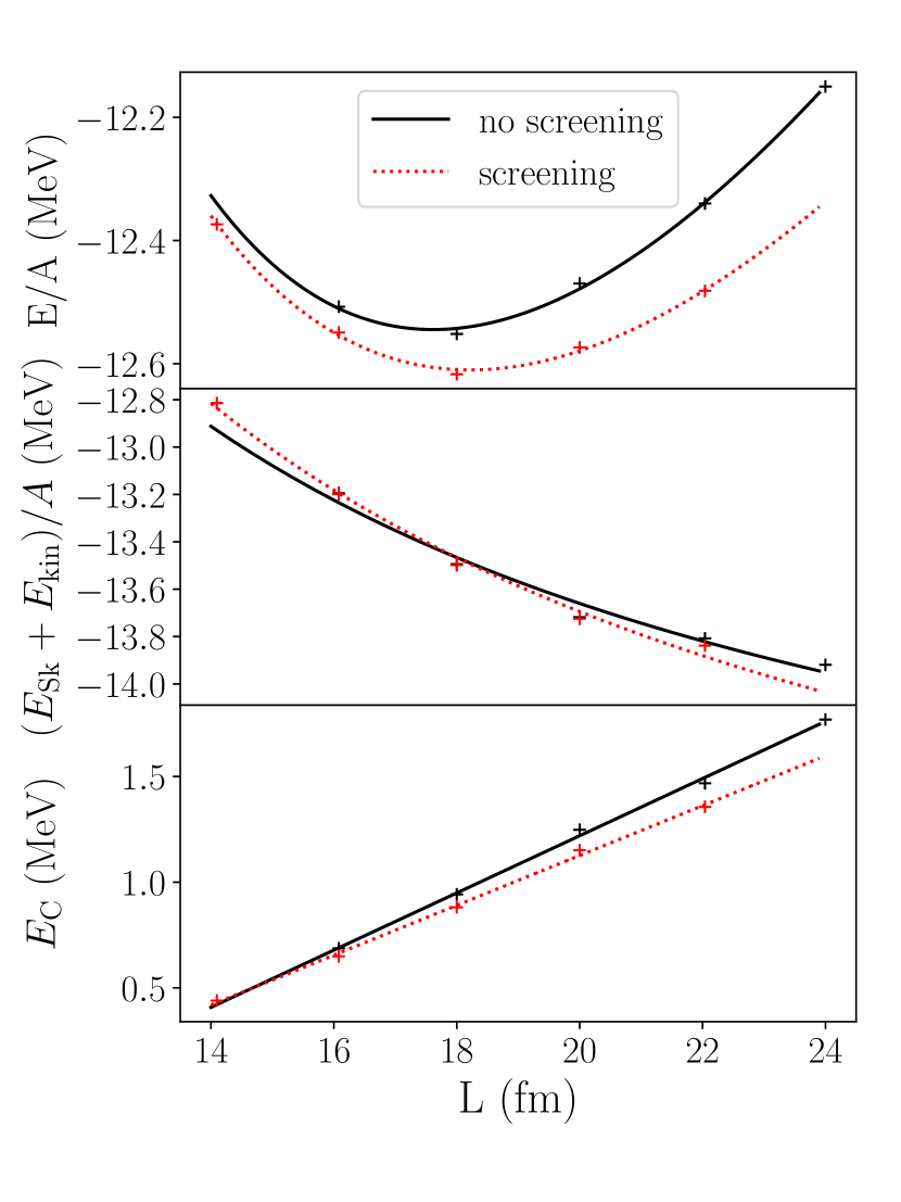
Figure 9: Total energy (top), Skyrme and kinetic energy (middle), and Coulomb energy (bottom) per nucleon for a slab configuration with $\rho=0.05\mathrm{\,fm}^{-3}$ and $X_{P}=1/2$ without electron screening (black, solid line) and with electron screening (red, dotted line).

In Fig. 9, the comparison of calculations with and without screening is shown for $\rho=0.05\mathrm{\,fm}^{-3}$ and $X_{P}=1/2$. While the Skyrme and kinetic energy part only varies little, the Coulomb energy is systematically reduced after switching the screening effect on. This causes the total energy to also be reduced slightly. For the optimal periodic length, the total energy changes from $-12.54\mathrm{\,MeV}$ to $-12.61\mathrm{\,MeV}$, which is about a 0.4% reduction. The optimal periodic length itself changes from $17.61\mathrm{\,fm}$ to $18.22\mathrm{\,fm}$, which is a much larger relative change of 2.3%.

For the most extreme case with $\rho=0.08\mathrm{\,fm}^{-3}$ and $X_{P}=1/2$, we observe a comparable change in energy and a larger increase of the periodic length of 4.8%. We expect the impact to be much smaller for low proton fractions because of the smaller charge density and thus a much larger screening radius (see Fig. 2). Overall, we expect that the influence for the binding energy is negligible and an increase of the preferred periodic length of no more than 5%.

VI Computational Scaling

Extensive calculations have been performed for this work, and, to the best of our knowledge, they represent the largest nuclear DFT ground state calculations ever performed. While most of the calculations were executed on the LOEWE facility at the Goethe University Frankfurt, calculations for the plots of the computational scaling shown below were performed on Cori at NERSC (National Energy Research Scientific Computing Center) in Berkeley, California. Cori - Phase I is a Cray XC40 supercomputing platform that consists of 4766 compute nodes, each with two 16-core Xeon E5-2698 v3 Haswell CPUs.

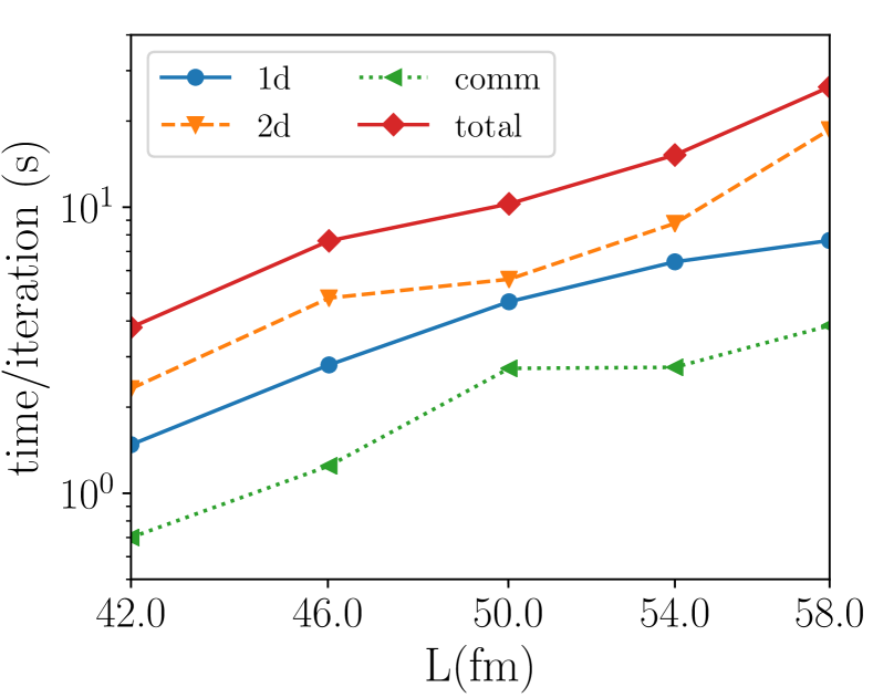
Figure 10: Total execution time per iteration using 512 cores for a system with $X_{P}=1/3$, $\rho=0.04$ with varying box lengths. The 1d part stands for evolving the wave function with the damped gradient step and the 2d part stands for the orthonormalization and diagonalization of the Hamiltonian. “Comm” marks the communication overhead. For details see Afibuzzaman et al. (2018)

.

First we present the scaling results with a fixed core count of 512 for a system with $X_{P}=1/3$ and $\rho=0.04$ for different box sizes in Fig. 10. We take a cubic box with 40 grid points in each direction for $L=42\mathrm{\,fm}$, 44 for $L=46\mathrm{\,fm}$, 48 for $L=50\mathrm{\,fm}$ and 50 for the larger boxes. We would expect a linear scaling with total grid points, if the number of wave functions was constant, because the FFT part, scaling with $N\log(N)$, does not take a considerable amount of time. The number of wave functions is determined by the density and thus increases as $V=L^{3}$.

The total computational time per iteration is divided into three parts. “2d” labels the part where the data (wave functions, matrices, etc.) are distributed over the CPU cores in a block cyclic 2d way. In this distribution the wave functions are orthonormalized and diagonalized w.r.t. the single-particle Hamiltonian. “1d” labels the part where the wave functions are distributed linearly over the CPU core. In that distribution every thread handles a number of wave functions. In that distribution the damped-gradient steps are performed. “comm” labels the time needed to switch between distributions.

The 2d part of the calculation is the most expensive part and is expected to scale with $(\text{number of s.p. wave functions})^{2}$. The 1d part is expected to be linearly dependent on the number of wave functions. In summary, we achieve the expected scaling. Going from the system with $L=42\mathrm{\,fm}$ to the system with $L=58\mathrm{\,fm}$, the computational time increases by a factor of about 7.

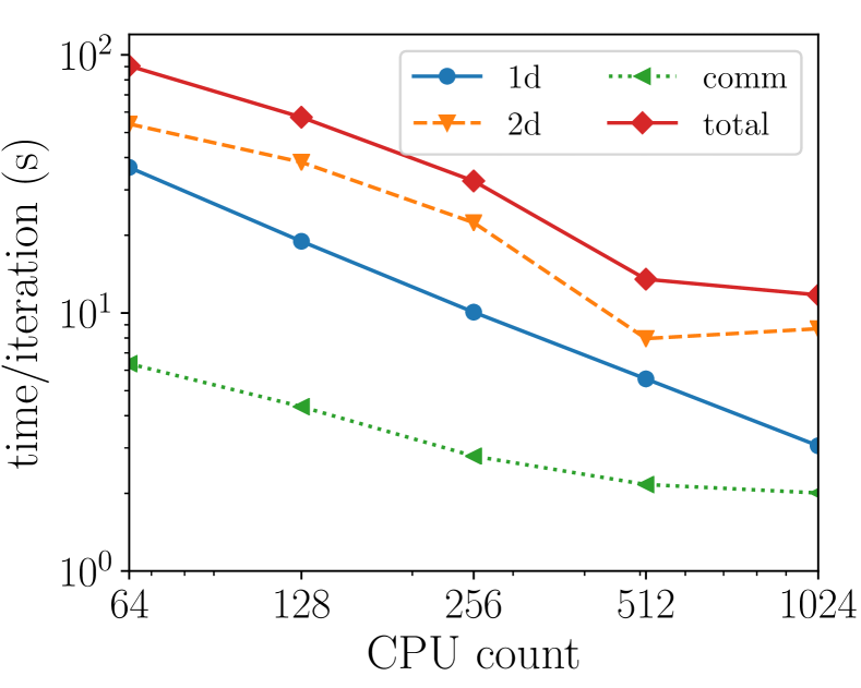
Figure 11: Same as Fig 10 but for a system with $L=46\mathrm{\,fm}$, $\rho=0.08$ and $X_{P}=1/2$ varying the core count.

In Fig. 11, we show the time per iteration for a fixed system with about 8000 particle wave functions with respect to the core count used. Note that for one node with 32 cores the memory was not sufficient for this large calculation. While the 1d part scales almost perfectly, the dominant 2d part is sensitive to the exact core count. The communication overhead is small and decreases with an increasing number of cores, but becomes comparable to the 1d part for large core counts. Overall, we again obtain a reasonable scaling. In practice, we use mostly 128 cores for smaller cases and 256 or 512 cores for large calculations ($L>40\mathrm{\,fm}$).

VII Conclusion

We studied single and double TPMS pasta configurations in comparison to the slab configuration at intermediate densities with less than half saturation density. As an interaction model, we chose the TOV-min parametrization, which has been fitted also to the mass radius relation of neutron stars. From the large difference of the energy per nucleon of uniform matter to pasta matter at $X_{P}=1/2$ and $1/3$, we can infer that pasta matter should be realized. Also for $X_{P}=1/10$ and low densities pasta significantly reduces the energy per nucleon.

The TPMS configuration cover a large span of different periodic lengths. Although the shapes are very different, physical properties such as the surface area per volume and Euler characteristic per volume reduce to almost the same values in the physical box scales. The energies per nucleon of the different configurations lie within a few hundred keV and thus if the temperature of the system exceeds this difference, several of the configurations can be present at the same time. We therefore expect that pasta matter at finite temperature is not well ordered, but undergoes constant transformation between different configurations and has amorphous character.

The analysis with finite temperature revealed that for a high proton fraction pasta matter can exist with temperatures $T>10\mathrm{\,MeV}$. For low proton fraction as e.g. present in a neutron star, pasta dissolves at still appreciable but lower temperatures. The preferred box lengths, however, can vary significantly.

We also looked at the impact of electron screening. While the change of the energy per nucleon is negligible and below the uncertainty of the nuclear interaction model, it can have a small influence on the periodic length of the configurations. Contrary to the common intuition, periodic lengths grow when including electron screening.