Understanding the mechanisms of electroplasticity from a crystal plasticity perspective

Abstract

Electroplasticity is defined as the reduction in flow stress of a material undergoing deformation on passing an electrical pulse through it. The lowering of flow stress during electrical pulsing has been attributed to a combination of three mechanisms: softening due to Joule-heating of the material, de-pinning of dislocations from paramagnetic obstacles, and the electron-wind force acting on dislocations. However, there is no consensus in literature regarding the relative magnitudes of the reductions in flow stress resulting from each of these mechanisms. In this paper, we extend a dislocation density based crystal plasticity model to incorporate the mechanisms of electroplasticity and perform simulations where a single electrical pulse is applied during compressive deformation of a polycrystalline FCC material with random texture. We analyze the reductions in flow stress to understand the relative importance of the different mechanisms of electroplasticity and delineate their dependencies on the various parameters related to electrical pulsing and dislocation motion. Our study establishes that the reductions in flow stress are largely due to the mechanisms of de-pinning of dislocations from paramagnetic obstacles and Joule-heating, with their relative dominance determined by the specific choice of crystal plasticity parameters corresponding to the particular material of interest.

1 Introduction

Electroplasticity (henceforth called as “EP”) is the phenomenon where a material undergoing deformation displays a drop in flow stress whenever subjected to an electrical pulse. The discovery of this phenomenon can be credited to Troitskii and Likhtman [1] who first observed the reductions in flow stress while passing current pulses through Zn single crystals. Since then it has been recognized that repeated application of the electrical pulses in quick succession during deformation lower the flow stress not only during the pulses but also between the pulses [2, 3, 4]. Thus, repeated electropulsing during deformation mimics the attributes of hot working, albeit at a much lower energy cost. This has prompted development of industrial manufacturing paradigms like Electrically-assisted manufacturing (EAM) and Electroplastic manufacturing processing (EPMP) which leverage the phenomenon of EP on an industrial scale. There are several reviews of EAM, EPMP, and the phenomenon of EP which can serve as useful references in this regard [5, 6, 7, 8].

Even as there are increased efforts to harness the benefits of EP in the manufacturing industry, the mechanisms contributing to EP continue to be poorly understood. Researchers over the years have proposed several different theories to explain the reductions in flow stress during electropulsing but without achieving any consensus about the mechanism which dominates the phenomenon of EP. The earliest theory to explain the electroplastic softening is that of Joule-heating; the electrical energy passed to the material is converted to heat, leading to thermal softening of the material. This is the simplest explanation of EP but it is far from being unanimously accepted. Several experiments report the temperature rise due to a single electrical pulse to be too small to be commensurate with the reductions in flow stress [5, 9, 10], while some later studies attribute the observed softening during electropulsing solely to Joule-heating [11, 12]. The ambiguity surrounding Joule heating as the dominant mechanism for EP prompted development of theories which could explain the reductions in flow stress without invoking a rise in temperature of the material. Conrad and co-workers [5, 9], present the first among the athermal theories, which is based on the transfer of momentum from the flowing electrons to the dislocations. It is also known as the “electron-wind force” theory and was conjectured to be the principal contributor to EP till Molotskii et al., [13] presented an analysis which demonstrated its effect to be small compared to the reductions in flow stress observed during experiments. Molotskii and co-workers [13, 14] also present a different explanation for the reductions in flow stress. They claim that the induced magnetic field due to the applied current alter the electronic states of the bonds between the obstacles and the dislocation cores which promote de-pinning of dislocations from such obstacles. Their theory requires the obstacles to be paramagnetic in character. The most prominent example of such obstacles are forest dislocations [15], which constitute one of the biggest contributors to flow hardening. Molotskii et al., [13, 14] also present an analysis of the reductions in flow stress due to such an effect and find the softening to be quite substantial compared to the two earlier mechanisms.

To date, the theories of Joule-heating, electron-wind force, and de-pinning from paramagnetic obstacles are the most commonly invoked explanations for instances of EP observed in different materials. The lack of agreement within the scientific community as to which mechanism dominates the electroplastic behaviour is partly because of the difficulty involved in experimentally validating the de-pinning of dislocations and the electron-wind force on dislocations due to electropulsing. There are in-situ TEM studies where dislocation motion is observed during electropulsing of thin-films [16, 17]. But more recent studies [18, 19] claim that no difference in dislocation activity is observed under current pulsing. It has to be noted that in all these observations there is no concurrent applied strain while electropulsing. Thus, in these studies, the imaged dislocations are static while the current pulses are applied and hence the tests may fail to recognize whether larger segments of dislocations have been freed due to de-pinning. Similarly, the validity of the electron-wind force theory also cannot be ascertained with certainty through such experiments as the transfer of momentum from the electrons to the dislocations may not constitute a high enough force by itself to cause dislocation motion.

With there being no clear understanding of the relative magnitudes of softening induced by different mechanisms of EP through experiments, modeling could play a key role in resolving this issue. There exists several crystal plasticity studies in literature which have tried to model electrically assisted forming [20, 21, 22, 23, 24]. In a couple of such studies [21, 24] constitutive models are presented which explain the envelope of the global stress-strain curve during frequent electropulsing without modeling the reductions in flow stress during electropulsing. The global softening of the material is captured phenomenologically without the consideration of any physical mechanisms other than Joule-heating. On the other hand, in [22, 23], the reductions in flow stress during pulsing are also modeled along with the global softening of the material due to repeated electropulsing. These phenomenological crystal plasticity models only allow an empirical consideration of the softening due to Joule-heating and electron-dislocation interactions and do not consider any particular athermal mechanism of softening. As these models do not implement the possible mechanisms of EP explicitly, the questions regarding the relative importance of the proposed mechanisms continue to remain unresolved.

In this paper, our objective is to understand the relative importance of the three theories of EP, namely, thermal softening, electron-wind force, and paramagnetic depinning of dislocations, in producing the reductions in flow stress during electropulsing. In order to achieve this, we employ a dislocation density based crystal plasticity model and extend it to include the different mechanisms proposed for EP. We then perform simulations of uniaxial compression of a representative polycrystalline sample where we pass a single electrical pulse during the loading process and analyze the reduction in flow stress achieved when each of these mechanisms is active. This allows us to develop an understanding of the reductions in flow stress caused by each of these mechanisms and we probe their dependencies on relevant parameters of the crystal plasticity model. A major novelty of our approach from the previous attempts at modeling EP is the fact that we use a dislocation density based crystal plasticity model which provides a physical framework for the introduction of the mechanisms of EP, in contrast to the phenomenological and empirical approaches of earlier studies. This also means that the crystal plasticity parameters employed in our study have a physical significance and can be determined from literature. We utilize this flexibility to select a parameter set for our simulations which is representative of a generic FCC material and hence our conclusions are not limited to any one particular material displaying EP. Our paper is organized in the following manner. First, we present the crystal plasticity model, which is followed by sections which extend the model to include athermal and thermal (Joule-heating) mechanisms of EP. We then present our results, following which we discuss the implications of our study and lay out the possibilities for generalizing the model further to materials belonging to other crystal structures.

2 Crystal plasticity model

We will be using a dislocation density based crystal plasticity model which is described in detail by Wong et al., [25]. As discussed in the previous section, all the mechanisms of EP are mediated exclusively by dislocation motion. So, in our discussion, we are not going to invoke the other mechanisms which contribute to plasticity, e.g., twinning and transformation induced plasticity (TWIP, TRIP). Our discussion will begin with a review of the kinematic and constitutive relationships of the model.

2.1 Kinematic and constitutive relationships

The imposed deformation gradient $\bm{F}$ is decomposed into elastic ($\bm{F_{e}}$) and plastic ($\bm{F_{p}}$) contributions following [26],

$$\bm{F}=\bm{F_{e}F_{p}}.$$ (1)

The stress is computed from the elastic strain by assuming a linear elastic material,

$$\bm{S}=\mathbb{C}\left(\bm{F_{e}}^{T}\bm{F_{e}}-\bm{I}\right)/2,$$ (2)

where, $\bm{S}$ is the second Piola-Kirchhoff stress tensor and $\mathbb{C}$ is the elastic tensor. The plastic velocity gradient ($\bm{L_{p}}$) for a single grain is determined by the stress tensor ($\bm{S}$) and the variables which define the microstructure ($\bm{\xi}$) as,

$$\bm{L_{p}}=\sum_{\alpha=1}^{N_{s}}\dot{\gamma^{\alpha}}\left(\bm{S,\xi}\right)\bm{m^{\alpha}}\otimes\bm{n^{\alpha}},$$ (3)

where $\bm{m^{\alpha}}$ denotes the slip direction and $\bm{n^{\alpha}}$ denotes the slip plane normal of the slip system $\alpha$. $\dot{\gamma^{\alpha}}$ denote the shear rates on the individual slip systems denoted by $\alpha$. $N_{s}$ denotes the total number of slip systems. The exact form of the dependence of $\dot{\gamma^{\alpha}}$ on $\bm{S}$ and $\bm{\xi}$ will be delineated in the next subsection. As discussed earlier, Eq. 3 considers dislocation motion to be the sole mechanism responsible for plasticity. $\bm{L_{p}}$ governs the evolution of the plastic deformation gradient through,

$$\dot{\bm{F_{p}}}=\bm{L_{p}F_{p}},$$ (4)

where, $\dot{\bm{F_{p}}}$ denotes the rate of change of the plastic deformation gradient with time. The  eqs. 1, 2, 3 and 4, can be combined to write,

$$\bm{P(x)}=\bm{F}\bm{S}=\bm{f\left(x,F,\xi\right)},$$ (5)

where, $\bm{P}$ is the first Piola-Kirchhoff stress tensor determined from $\bm{S}$. Eq. 5 is the crux of the crystal plasticity model and is coupled to the balance of linear momentum through,

$$\nabla\cdot\bm{P}=0,$$ (6)

to simulate a Representative Volume Element (RVE) under static equilibrium. The numerical schemes employed to solve these equations are described in detail elsewhere [27].

2.2 Microstructure ($\xi$) and shear rates $\dot{\gamma^{\alpha}}$

The microstructure ($\bm{\xi}$) of the material is described by the mobile edge dislocation density denoted by $\rho_{m}$ and the immobile dipole dislocation density $\rho_{d}$. The motion of the mobile dislocations determines the shear rate $\dot{\gamma^{\alpha}}$ on the slip system $\alpha$, as given by the Orowan equation,

$$\dot{\gamma^{\alpha}}=\rho_{m}^{\alpha}b_{s}v_{0}\exp\left[-\dfrac{Q_{s}}{k_{\text{B}}T}\left\{1-\left(\dfrac{\tau_{eff}^{\alpha}}{\tau_{sol}}\right)^{p}\right\}^{q}\right]\textrm{sign}(\tau^{\alpha}),$$ (7)

which assumes dislocation glide to be controlled by thermal activation. In Eq. 7, $\rho_{m}^{\alpha}$ denotes the mobile dislocation density in the slip system $\alpha$, $Q_{s}$ is the activation energy for slip, $b_{s}$ is the magnitude of the Burgers vector, $k_{\text{B}}$ represents the Boltzmann constant and $T$ is the temperature, $\tau_{sol}$ is the stress required to overcome short range obstacles at $0K$, $v_{0}$ is the dislocation glide velocity prefactor. $\tau_{eff}^{\alpha}$ is the effective resolved shear stress written as, $\tau_{eff}^{\alpha}=|\tau^{\alpha}|-\tau_{pass}^{\alpha}$, when $|\tau^{\alpha}|>\tau_{pass}^{\alpha}$, and $\tau_{eff}^{\alpha}=0$, otherwise. $\tau^{\alpha}$ is the resolved applied shear stress on the slip system $\alpha$ given by $\tau^{\alpha}={\bm{F_{e}}}^{T}\bm{F_{e}}\bm{S}\left({\bm{m}}^{\alpha}\otimes{\bm{n}}^{\alpha}\right)$ and $\tau_{pass}^{\alpha}$ is the passing stress experienced by the mobile dislocations in the slip system $\alpha$, due to the long range elastic strain fields of the dislocations, defined as,

$$\tau_{pass}^{\alpha}=Gb_{s}\left[\sum_{{\alpha^{\prime}}=1}^{N_{s}}\xi_{\alpha\alpha^{\prime}}\left(\rho_{e}^{\alpha^{\prime}}+\rho_{d}^{\alpha^{\prime}}\right)\right]^{1/2},$$ (8)

where, $G$ is the shear modulus, and $\xi_{\alpha\alpha^{\prime}}$ is the interaction matrix of the slip systems. It is important to note that the first instance when $|\tau^{\alpha}|$ is greater than $\tau_{pass}^{\alpha}$ defines yielding on the slip system $\alpha$, where the corresponding value of $\tau_{pass}^{\alpha}$ is the slip system level yield stress. $\rho_{m}^{\alpha^{\prime}}$ and $\rho_{d}^{\alpha^{\prime}}$ are the mobile edge and immobile dipole dislocation densities, respectively, whose evolutions are governed by,

$$\dot{\rho}_{m}^{\alpha}=\dfrac{|\dot{\gamma}^{\alpha}|}{b_{s}\Lambda_{s}^{\alpha}}-\dfrac{2\hat{d}^{\alpha}}{b_{s}}\rho_{m}^{\alpha}|\dot{\gamma^{\alpha}}|-\dfrac{2\check{d}^{\alpha}}{b_{s}}\rho_{m}^{\alpha}|\dot{\gamma^{\alpha}}|,$$ (9)

and,

$$\dot{\rho}_{d}^{\alpha}=\dfrac{2\hat{d}^{\alpha}}{b_{s}}\rho_{m}^{\alpha}|\dot{\gamma^{\alpha}}|-\dfrac{2\check{d}^{\alpha}}{b_{s}}\rho_{d}^{\alpha}|\dot{\gamma^{\alpha}}|-\rho_{d}^{\alpha}\dfrac{4v_{climb}}{\hat{d}^{\alpha}-\check{d}^{\alpha}},$$ (10)

respectively. $\Lambda_{s}^{\alpha}$ is the mean free path of dislocations. The maximum separation of the glide planes that allow dislocations gliding on them to form dipoles is $\hat{d^{\alpha}}$ while two edge dislocations would get annihilated whenever they are any closer to each other than $\check{d^{\alpha}}$. These distances are calculated to be,

$$\hat{d^{\alpha}}=\dfrac{3Gb_{s}}{16\pi|\tau^{\alpha}|},$$ (11)

and,

$$\check{d^{\alpha}}=C_{anni}b_{s},$$ (12)

where, $C_{anni}$ is a fitting parameter. The dislocation climb velocity $v_{climb}$ is given by,

$$v_{climb}=\dfrac{3GD_{0}\Omega}{2\pi k_{\text{B}}T}\dfrac{1}{\left(\hat{d^{\alpha}}+\check{d^{\alpha}}\right)}\exp\left(-\dfrac{Q_{c}}{k_{\text{B}}T}\right),$$ (13)

where $D_{0}$ is the self diffusion coefficient of the material in question, $\Omega$ and $Q_{c}$ are the activation volume and activation energy for climb, respectively. The mean free path $\Lambda_{s}^{\alpha}$ is defined as,

$$\dfrac{1}{\Lambda_{s}^{\alpha}}=\dfrac{1}{d}+\dfrac{1}{\lambda_{slip}^{\alpha}},$$ (14)

where $d$ is the grain size and $\lambda_{slip}^{\alpha}$ is the average distance traveled by a dislocation before it is stopped by forest dislocations, written as,

$$\dfrac{1}{\lambda_{slip}^{\alpha}}=\dfrac{1}{i_{slip}}\left[\sum_{{\alpha^{\prime}}=1}^{N_{s}}\xi_{\alpha\alpha^{\prime}}\left(\rho_{m}^{\alpha^{\prime}}+\rho_{d}^{\alpha^{\prime}}\right)\right]^{1/2},$$ (15)

where $i_{slip}$ is a fitting parameter.

3 Athermal mechanisms of EP

In this section we discuss the major theories explaining EP which do not rely on thermal softening of the material due to Joule heating. We begin with a discussion of the theories by Molotskii and co-workers which involve de-pinning of dislocations from obstacles during electropulsing. We follow that up with a review of the theory of electron-wind force assisted dislocation glide as put forth by Conrad and co-workers. While considering each of these mechanisms we will also lay out the extensions to the crystal plasticity model required to implement them and attempt a theoretical analysis of the reductions in flow stress caused by each of them wherever possible.

3.1 Paramagnetic de-pinning of dislocations

Molotskii and Fleurov [13] in their seminal paper suggested that de-pinning of dislocations from paramagnetic obstacles is the dominant softening mechanism during electrical pulsing. They demonstrate that the induced magnetic field due to electrical pulsing alters the electronic states in the obstacles and the dislocation cores. These modified electronic states result in a much lower probability of the dislocations being pinned by such obstacles. Forest dislocations qualify as paramagnetic obstacles [15] and they constitute the largest fraction of short range obstacles encountered by dislocations in FCC materials. Thus, any gain in plasticity due to a change in the pinning behaviour of such obstacles is likely to be very significant.

It must be noted that the mechanism of de-pinning of dislocations is not dependent on the sense of the current density vector $\bm{j}$, but only on its magnitude $j=|\bm{j}|$. So, in this section, whenever we use “current density” we mean its magnitude represented by $j$.

In view of the crystal plasticity model we have described in Section 2, reductions in flow stress due to de-pinning of dislocations can manifest through several terms in Eq. 7. We will refer to them as “sources” of softening within the purview of the primary mechanism of de-pinning of dislocations from paramagnetic obstacles. We investigate each of the sources in the following sub-sections.

3.1.1 Effect of a change in $\tau_{sol}$

As proposed by Molotskii and co-workers [13, 14], during the application of an electrical pulse, the pinning of dislocations by short range obstacles are weakened. This implies that the inter-obstacle spacing $l_{c}(0)$ while no current is passed increases to a new value $l_{c}(j)$ under pulsing. The inter-obstacle distance ($l_{c}$) changes as a function of the imposed current density ($j$) as [13],

$$l_{c}(j)=l_{c}(0)\left(1+\dfrac{j^{2}}{j_{0}^{2}}\right),$$ (16)

where, $j_{0}$ is a characteristic current density magnitude which corresponds to the magnitude of current density $j$ at which the EP is typically observed for a particular material.

The change in $l_{c}$ will affect the parameter $\tau_{sol}$ in Eq. 7. $\tau_{sol}$ represents the short range resistance experienced by an average dislocation segment. Following the analysis in [28], $\tau_{sol}$ scales inversely as the separation between the short range obstacles. In other words,

$$\tau_{sol}\propto\dfrac{1}{l_{c}}.$$ (17)

Combining Eqs. 16 and 17 we can write $\tau_{sol}$ as a function of $j$ as,

$$\tau_{sol}(j)=\dfrac{\tau_{sol}(0)}{\left(1+\dfrac{j^{2}}{j_{0}^{2}}\right)}.$$ (18)

Under electropulsing the shear rate on any particular slip system $\alpha$ can be written as,

$$\dot{\gamma^{\alpha}}(j)=\rho_{m}^{\alpha}b_{s}v_{0}\exp\left[-\dfrac{Q_{s}}{k_{\text{B}}T}\left\{1-\left(\dfrac{\tau_{eff}^{\alpha}(j)}{\tau_{sol}(j)}\right)^{p}\right\}^{q}\right]\textrm{sign}(\tau^{\alpha}).$$ (19)

The lowering of $\tau_{sol}$ represents lowering of the short range obstacle strength. Thus, under pulsing, similar shear rates ($\dot{\gamma^{\alpha}}$) can be maintained by smaller effective resolved shear stresses $\tau_{eff}^{\alpha}$ and consequently by $\tau^{\alpha}$ which explain the reductions in flow stress on the level of individual slip systems. Thus, the dependence of $\tau_{sol}$ on $j$ (Eq. 18), leads to $\tau_{eff}^{\alpha}$ being a function of $j$ in Eq. 19.

Molotskii and Fleurov[13] also perform an analysis of the estimated stress drop due to such a softening mechanism. While our formulation of the electroplastic phenomena is on the slip system level, the analysis performed in [13] is for the bulk polycrystalline sample. In order to replicate a similar analysis employing our formulation, we relate the plastic behaviour of the bulk sample to that of a single grain employing the concept of Taylor factor ($M$),

$$\dot{\epsilon}(0)=\dfrac{1}{M}\sum_{\alpha=1}^{N_{s}}\dot{\gamma^{\alpha}}(0)$$

$$=\dfrac{1}{M}\sum_{\alpha=1}^{N_{s}}\Bigg{(}\rho_{m}^{\alpha}b_{s}v_{0}\cdot$$

$$\exp\left[-\dfrac{Q_{s}}{k_{\text{B}}T}\left\{1-{\left(\dfrac{(\sigma_{eff}(0)/M)}{\tau_{sol}(0)}\right)}^{p}\right\}^{q}\right]\Bigg{)}\textrm{sign}(\tau^{\alpha}),$$ (20)

where, $\alpha$ runs over all the slip systems in single grain. In Eq. 20 $\dot{\epsilon}$ is the imposed bulk strain rate and remains constant regardless of whether the system is pulsed or not and $\sigma_{eff}$ is the effective normal stress along the loading direction and can be thought of as the difference between the applied stress ($\sigma_{appl}$) and the long-range resistance ($\sigma_{pass}$) which are related to the corresponding quantities $\tau^{\alpha}$ and $\tau_{pass}^{\alpha}$, respectively, for a single slip system. Eq. 20, can be modified for an electropulsed sample in the following manner as,

$$\dot{\epsilon}(j)=\dfrac{1}{M}\sum_{\alpha}\dot{\gamma^{\alpha}}(j)$$

$$=\dfrac{1}{M}\sum_{\alpha}\Bigg{(}\rho_{m}^{\alpha}b_{s}v_{0}\cdot$$

$$\exp\left[-\dfrac{Q_{s}}{k_{\text{B}}T}\left\{1-{\left(\dfrac{(\sigma_{eff}(j)/M)}{\tau_{sol}(j)}\right)}^{p}\right\}^{q}\right]\Bigg{)}\textrm{sign}(\tau^{\alpha}).$$ (21)

We divide Eq. 21 by Eq. 20 and impose $\dot{\epsilon}(j)=\dot{\epsilon}(0)$, to write,

$$\sum_{\alpha}\rho_{m}^{\alpha}\exp\left[-\dfrac{Q_{s}}{k_{\text{B}}T}\left\{1-{\left(\dfrac{(\sigma_{eff}(0)/M)}{\tau_{sol}(0)}\right)}^{p}\right\}^{q}\right]\textrm{sign}(\tau^{\alpha})$$

$$=\sum_{\alpha}\rho_{m}^{\alpha}\exp\left[-\dfrac{Q_{s}}{k_{\text{B}}T}\left\{1-{\left(\dfrac{(\sigma_{eff}(j)/M)}{\tau_{sol}(j)}\right)}^{p}\right\}^{q}\right]\textrm{sign}(\tau^{\alpha}).$$ (22)

Noting that the arguments to the exponentials are not functions of $\alpha$, we can simplify Eq. 22 to get,

$$\dfrac{\sigma_{eff}(0)}{\tau_{sol}(0)}=\dfrac{\sigma_{eff}(j)}{\tau_{sol}(j)},$$ (23)

and using Eq. 18 this can be written as,

$$\Delta\sigma_{eff}=\sigma_{eff}(0)-\sigma_{eff}(j)=\sigma_{eff}(0)\dfrac{j^{2}}{j_{0}^{2}+j^{2}}.$$ (24)

$\Delta\sigma_{eff}$ is the difference in effective stresses recorded before and after electropulsing and we can relate it to the applied stress ($\sigma_{appl}$) by assuming the averaged long range elastic stress fields to remain constant ($\sigma_{pass}$) when $\tau_{sol}$ is modified due to electropulsing. So, in terms of the applied stresses,

$$\Delta\sigma_{appl}=\Delta\sigma_{eff}=\sigma_{eff}(0)\dfrac{j^{2}}{j_{0}^{2}+j^{2}}.$$ (25)

The above equation reveals interesting trends for very low and high values of $j$. For $j<<j_{0}$,

$$\Delta\sigma_{appl}\approx\sigma_{eff}(0)\dfrac{j^{2}}{j_{0}^{2}},$$ (26)

which reveals a parabolic dependence on $j$. When $j>>j_{0}$, we get,

$$\Delta\sigma_{appl}\approx\sigma_{eff}(0),$$ (27)

and so the stress drop saturates. The variation of $\Delta\sigma_{appl}$ as a function of $(j/j_{0})$ as predicted by Eq. 25 has a point of inflection where the curvature $(\partial^{2}\Delta\sigma_{appl}/\partial j^{2})$ changes from positive to negative and it happens at $(j/j_{0})=1/\sqrt{3}=0.577$, which marks a transition between the regimes denoted by Eqs. 26 and 27.

It is also important to take note of the assumptions made to arrive at Eq. 25. The one central assumption of the analysis is that the effective resolved shear stresses $\tau_{eff}^{\alpha}$ are the same for all the slip systems ($\alpha$). This assumption allows us to introduce the Taylor factor($M$) in Eq. 20. For crystal plasticity simulations of bulk polycrystalline materials an equality of $\tau_{eff}^{\alpha}$ for all the slip systems for any particular grain is uncommon and there are considerable differences across the slip systems over all the grains. Also, it has even been observed that the number of active slip systems ($|\tau^{\alpha}|>\tau_{pass}^{\alpha}$) may vary from $3$ to $9$ per grain in a polycrystalline sample and all the grains do not deform similarly as conjectured by Taylor’s theory [29]. So, in view of these differences with crystal plasticity implementations, it is reasonable to expect differences between the predictions from simulations and the simplified analysis.

While considering a lowered short-range obstacle strength, Molotskii and co-workers ignored other potential ramifications of the de-pinning of dislocations from paramagnetic obstacles. In the next few subsections, we will explore other possible consequences of dislocation de-pinning within the crystal plasticity framework we have introduced.

3.1.2 Effect of a change in $\lambda_{slip}^{\alpha}$

Another possible effect of the de-pinning of dislocations is an increase of the distance traveled by the dislocation before being trapped by the forest dislocations ($\lambda_{slip}^{\alpha}$). $\lambda_{slip}^{\alpha}$ should be scaled by the same factor $(1+j^{2}/j_{0}^{2})$ which depicts the scaling of the distance between the trapping points due to the forest dislocations. Hence, we can write from Eq. 15,

$$\lambda_{slip}^{\alpha}(j)=\lambda_{slip}^{\alpha}(0)\left(1+\dfrac{j^{2}}{j_{0}^{2}}\right)$$ (28)

The effect of change in this length scale on the applied stress is complicated. It alters the evolution of the dislocation densities through Eq. 9 which in turn can affect the passing stress $\tau_{pass}^{\alpha}$ as given in Eq. 8. As $\lambda_{slip}^{\alpha}$ does not explicitly appear in the Orowan equation an analytical expression relating it to the reductions in flow stress is intractable. However, it is worthwhile to develop an intuitive understanding of the kind of changes prompted in $\rho_{m}^{\alpha}$ and $\tau_{pass}^{\alpha}$ due to a change in $\lambda_{slip}^{\alpha}$. From Eqs. 9 and 14 it is clear that $\rho_{m}^{\alpha}$ would increase at a slower rate when $\lambda_{slip}^{\alpha}$ is larger. Under the assumption that $\dot{\epsilon(0)}=\dot{\epsilon(j)}$, implies $\dot{\gamma^{\alpha}}(0)=\dot{\gamma^{\alpha}}(j)$, a smaller $\rho_{m}^{\alpha}$ necessitates a larger $\tau_{eff}^{\alpha}$ to maintain a constant $\dot{\gamma^{\alpha}}$. A higher $\tau_{eff}^{\alpha}$ can be achieved either by lowering of $\tau_{pass}^{\alpha}$ or by a higher resolved shear stress ($\tau^{\alpha}$). The former can lead to flow softening while the latter can lead to a stress rise during electropulsing and the net change is a combined effect of the two. Thus, there is a possibility of a rise in flow stress instead of a drop due to an increase of $\lambda_{slip}^{\alpha}$.

3.1.3 Effect of a change in $v_{0}$

From the expression of the Orowan equation presented in Eq. 7, the velocity of dislocations can be expressed as a product of the velocity prefactor $v_{0}$ and an Arrhenius term, given as,

$$v=v_{0}\exp\left[-\dfrac{Q_{s}}{k_{\text{B}}T}\left\{1-\left(\dfrac{\tau_{eff}^{\alpha}}{\tau_{sol}}\right)^{p}\right\}^{q}\right],$$ (29)

where,

$$v_{0}=\nu_{G}\,d_{s},$$ (30)

where $\nu_{G}$ is the jump frequency of the dislocations and $d_{s}$ is the distance moved forward per successful thermal activation event. Granato et al., [30] suggest that $\nu_{G}$ is independent of the free length of the dislocations between two obstacles and so should remain constant as the odds of pinning by obstacles lower while electropulsing. As an obstacle is overcome by thermal activation, the freed dislocation segment glides until it encounters another obstacle, after which the entire process of thermal activation is repeated. From that argument, we have $d_{s}=l_{c}$. Thus, under electropulsing, it is reasonable to expect that dislocations would glide larger distances as pinning is less probable. Using the variation of $l_{c}(j)$ as given by Eq. 16 we can write the corresponding scaling relationship for $d_{s}$ as,

$$d_{s}(j)=d_{s}(0)\left(1+\dfrac{j^{2}}{j_{0}^{2}}\right).$$ (31)

Combining Eqs. 30 and 31 we get a scaling relationship for $v_{0}$ as given by,

$$v_{0}(j)=v_{0}(0)\left(1+\dfrac{j^{2}}{j_{0}^{2}}\right).$$ (32)

An analysis similar to that done for the reductions in flow stress due to $\tau_{sol}$ when carried out for this case results in an expression which reads,

$$\Delta\sigma_{appl}=\Delta\sigma_{eff}=M\tau_{sol}\left(\dfrac{k_{\text{B}}T}{Q_{s}}\right)\log\left(1+\dfrac{j^{2}}{j_{0}^{2}}\right),$$ (33)

where, we have assumed $\sigma_{pass}$ to be unaffected by a change in $v_{0}$ during pulsing. For situations where $j/j_{0}<<1$, Eq. 33 can be approximated as,

$$\Delta\sigma_{appl}=\Delta\sigma_{eff}=M\tau_{sol}\left(\dfrac{k_{\text{B}}T}{Q_{s}}\right)\dfrac{j^{2}}{j_{0}^{2}}.$$ (34)

3.1.4 Effect of a change in passing stress $\tau_{pass}^{\alpha}$

Molotskii and Fleurov [31] argue that as the dislocations are de-pinned from short range obstacles, they have a larger free length and hence have a larger geometrical freedom to rotate and re-orient to the long range elastic stress fields of other dislocations. Thus, under electropulsing, dislocations can achieve configurations which minimize the strain energy more effectively compared to the situation where no electrical pulses are applied. This implies that larger stresses are needed to force dislocation motion while being pulsed and is an anomaly considering that all other mechanisms induce softening of the material. In the context of the crystal plasticity model described in the paper, $\tau_{pass}^{\alpha}$ represents the resistance to dislocation motion from the long range strain fields and it should be modified to describe this particular phenomenon. Following the analysis of Molotskii and Fleurov [31] we can modify Eq. 8 as,

$$\tau_{pass}^{\alpha}=\delta Gb_{s}\left[\sum_{{\alpha^{\prime}}=1}^{N_{s}}\xi_{\alpha\alpha^{\prime}}\left(\rho_{m}^{\alpha^{\prime}}+\rho_{d}^{\alpha^{\prime}}\right)\right]^{1/2},$$ (35)

where, a factor $\delta$ is introduced to account for the enhanced elastic interaction. $\delta$ is conjectured to have a form given by the following expansion [31],

$$\delta =1+\beta\left(\dfrac{l_{c}(j)-l_{c}(0)}{l_{c}(0)}\right)+\cdots,$$

$$=1+\beta\dfrac{j^{2}}{j_{0}^{2}},$$ (36)

restricting consideration to the first order terms only. In Eq. 36 $\beta$ is a constant determined by fitting and we have made use of Eq. 16 to arrive to the final form.

We can derive an expression for reductions in flow stress (or increases in flow stress in this case) $\Delta\sigma_{appl}$ corresponding to the enhanced work hardening due to electropulsing. Following the approach undertaken to derive Eq. 23, a corresponding relationship for this case is written as,

$$\sigma_{eff}(j)=\sigma_{eff}(0),$$ (37)

which leads to,

$$\Delta\sigma_{appl}=\Delta\sigma_{pass}=-\sigma_{pass}(0)\beta\dfrac{j^{2}}{j_{0}^{2}},$$ (38)

where we have assumed $M\tau_{pass}^{\alpha}=\sigma_{pass}$, $M$ being the Taylor factor. The negative sign in the RHS of Eq. 38 confirms that the applied stresses would need to be increased when such an effect is operative.

It is important that to note $\beta$ can be determined by fitting Eq. 35 to the variation of yield stresses in the material as a function of the imposed current density $j$ [31]. The yield stress of the material corresponds to the value of $\sigma_{pass}$ when $\sigma_{applied}$ overcomes $\sigma_{pass}$ for the first time. Such a quantity is not modified by any other softening mechanism operative due to de-pinning of dislocations and hence is suitable for determining $\beta$.

We have considered all possible manifestations of the phenomenon of de-pinning of dislocations during electropulsing. Also, we have presented extensions to the crystal plasticity model which will allow us to simulate the effects of these mechanisms in the later sections. We will discuss the theory of electron-wind force assisted dislocation motion next.

3.2 Electron-wind force: Conrad and co-workers

Conrad et al., [9] proposed a theory where the electrons drifting under the application of an electric field exert a force on the dislocations. This is known as “electron-wind” force and its expression derived by considering the scatter of electrons by dislocations can be stated as,

$$\bm{F_{ew}}=\dfrac{\rho_{D}}{N_{D}}en_{e}\bm{j},$$ (39)

where, $e$ is the electronic charge, $n_{e}$ is the density of free electrons, $\bm{j}$ is the current density and $\bm{F_{ew}}$ is the force per unit length of dislocations. In the crystal plasticity model described, plasticity is governed by the motion of the pure edge dislocations which move parallel to themselves along the slip direction $\bm{m^{\alpha}}$ in the particular slip systems ($\alpha$). In that case the component of the electron-wind force along the direction of the dislocation motion is given by $\bm{F_{ew}}\cdot\bm{m^{\alpha}}$. Assuming an equal fraction of positive and negatively signed dislocations in the material, it is apparent that if the electron-wind force aids the gliding dislocations of one particular sign then it should impede the motion of those belonging to the other sign. This is also pointed out by Molotskii and Fleurov[13] and it implies that the electron-wind force on dislocations is at best a second order effect.

Modeling the effects of the electron-wind force requires an alternate form of the Orowan equation (Eq. 7) written as,

$$\dot{\gamma^{\alpha}}=\rho_{m}^{\alpha}b_{s}v_{0}\exp\left[-\left(\dfrac{Q_{s}-\tau_{eff}^{\alpha}V}{k_{\text{B}}T}\right)\right]\textrm{sign}(\tau^{\alpha}),$$ (40)

where, the argument of the exponential has been written in an equivalent form assuming the following relationship,

$$\Delta G=Q_{s}-\tau_{eff}^{\alpha}V^{\alpha}=Q_{s}\left\{1-\left(\dfrac{\tau_{eff}^{\alpha}}{\tau_{sol}}\right)^{p}\right\}^{q},$$ (41)

with the Gibbs free-energy of activation denoted by $\Delta G$. The new parameter which appears in the modified Orowan equation (Eq. 40) is the activation volume of slip denoted by $V^{\alpha}$. The new form of the Orowan equation is necessitated to simplify the introduction of the electron-wind force. Following Conrad[9], the effect of the electron-wind force can be modeled as,

$$\dot{\gamma^{\alpha}} =\dfrac{1}{2}\rho_{m}^{\alpha}b_{s}v_{0}\Bigg{\{}\exp\left[-\left(\dfrac{Q_{s}-\tau_{eff}^{\alpha}V^{\alpha}-(\bm{F_{ew}}\cdot\bm{m^{\alpha}})A^{\alpha}}{k_{\text{B}}T}\right)\right]+$$

$$\exp\left[-\left(\dfrac{Q_{s}-\tau_{eff}^{\alpha}V^{\alpha}+(\bm{F_{ew}}\cdot\bm{m^{\alpha}})A^{\alpha}}{k_{\text{B}}T}\right)\right]\Bigg{\}}\textrm{sign}(\tau^{\alpha}),$$ (42)

where $A^{\alpha}$ denotes the activation area which is related to the activation volume ($V$) as, $V^{\alpha}=A^{\alpha}b_{s}$. Eq. 42 treats the electron-wind as an additional force on the dislocations similar to that exerted by $\tau_{eff}^{\alpha}$. The differential effect of the electron-wind force on dislocations of either sign manifests in Eq. 42 through opposite signs of the electron-wind force $(\bm{F_{ew}}\cdot\bm{m^{\alpha}})$ for the dislocation densities of either signs $(\rho_{m}^{\alpha}/2)$. The usefulness of the form of Eq. 40 is evident here as it allows the electron-wind force to be treated in a manner akin to the effective stress $\tau_{eff}^{\alpha}$. Eq. 42 can be simplified to obtain,

$$\dot{\gamma^{\alpha}}=\rho_{m}^{\alpha}b_{s}v_{0}\exp\left[-\left(\dfrac{Q_{s}-\tau_{eff}^{\alpha}(j)V^{\alpha}}{k_{\text{B}}T}\right)\right]$$

$$\cosh\left(\dfrac{(\bm{F_{ew}}\cdot\bm{m^{\alpha}})A}{k_{\text{B}}T}\right)\textrm{sign}(\tau^{\alpha}).$$ (43)

We are now in a position to revert back to the form of the Orowan equation as given by Eq. 7 to finally write,

$$\dot{\gamma^{\alpha}}=$$

$$\rho_{m}^{\alpha}b_{s}v_{0}\exp\left[-\dfrac{Q_{s}}{k_{\text{B}}T}\left\{1-\left(\dfrac{\tau_{eff}^{\alpha}(j)}{\tau_{sol}}\right)^{p}\right\}^{q}\right]$$

$$\cosh\left(\dfrac{(\bm{F_{ew}}\cdot\bm{m^{\alpha}})A}{k_{\text{B}}T}\right)\textrm{sign}(\tau^{\alpha}),$$ (44)

which indicates that the electron-wind force introduces the factor, $\cosh\left((\bm{(F_{ew}}\cdot\bm{m^{\alpha}})A)/(k_{\text{B}}T)\right)$, to the Orowan equation. For a situation where, $((\bm{F_{ew}}\cdot\bm{m^{\alpha}})A/(k_{\text{B}}T))<<1$, a Taylor-Series expansion writes as,

$$\cosh\left(\dfrac{(\bm{F_{ew}}\cdot\bm{m^{\alpha}})A}{k_{\text{B}}T}\right)=1+\dfrac{1}{2!}\left(\dfrac{(\bm{F_{ew}}\cdot\bm{m^{\alpha}})A}{k_{\text{B}}T}\right)^{2}+\cdots.$$ (45)

So, this indicates that in the event the electron-wind force is small, the factor introduced by it in the Orowan equation is of the second order.

An analytical approach to determine the dependence of reductions in flow stress on the current density ($j$) is not feasible due to the dependence of the electron-wind force on the direction of dislocation motion on individual slip planes. Such a dependence complicates deriving an analytical expression of the average electron-wind force over the entire bulk sample.

Conrad and co-workers [9] also claimed that the activation area $A^{\alpha}$ changes due to electropulsing. The activation area ($A^{\alpha}$) can be defined as [13],

$$A^{\alpha}=-\dfrac{1}{b_{s}}\dfrac{\partial\Delta G}{\partial\tau_{eff}^{\alpha}},$$ (46)

and using the last equality of Eq. 41 in Eq. 46, we get,

$$A^{\alpha}=\dfrac{Q_{s}}{\tau_{sol}b_{s}}pq\left\{1-\left(\dfrac{\tau_{eff}^{\alpha}}{\tau_{sol}}\right)^{p}\right\}^{(q-1)}\left(\dfrac{\tau_{eff}^{\alpha}}{\tau_{sol}}\right)^{(p-1)}.$$ (47)

From Eq. 47, it is clear that $A^{\alpha}$ increases under electropulsing as $\tau_{sol}$ is scaled down by a factor of $\left(1+\dfrac{j^{2}}{j_{0}^{2}}\right)$ following our implementation of Molotskii’s theory [13]. So, henceforth in our discussion we do not consider a change in $A^{\alpha}$ explicitly as such an effect is already included in the mechanism of a change in $\tau_{sol}$ causing softening.

4 Thermal softening due to Joule-heating

Another source of the reductions in flow stress during electropulsing is conjectured to be the thermal softening of the material due to Joule heating. In order to examine this particular source, we first solve the thermal conduction equation to determine the temperature ($T$),

$$\rho C_{p}\dot{T}=\nabla\cdot\left(\bm{K}\nabla T\right)+\dot{Q},$$ (48)

where, $\bm{K}$ is the thermal conductivity, $\rho$ is the density of the material, $C_{p}$ is the specific heat capacity, and $\dot{Q}$ is the source term per unit volume. The heat source term is computed as,

$$\dot{Q} =\bm{j}\cdot\bm{E},$$

$$=\bm{j}\cdot\left[{\bm{\sigma_{el}}}^{-1}\bm{j}\right],$$ (49)

where, we have used $\bm{j}=\bm{\sigma_{el}}\bm{E}$; $\bm{E}$ is the electric field vector and $\bm{\sigma_{el}}$ is the electrical conductivity tensor. The evolution of $T$ impacts the shear rates ($\dot{\gamma^{\alpha}}$) as given by,

$$\dot{\gamma^{\alpha}}=\rho_{m}^{\alpha}b_{s}v_{0}\exp\left[-\dfrac{Q_{s}}{k_{\text{B}}T(j)}\left\{1-\left(\dfrac{\tau_{eff}^{\alpha}(j)}{\tau_{sol}}\right)^{p}\right\}^{q}\right]\textrm{sign}(\tau^{\alpha}),$$ (50)

where $T$ is now a function of the imposed current density $j$. An analysis to determine the reductions in flow stress from thermal softening can be carried out in a manner similar to that done for the situation where $\tau_{sol}$ changes. In order to do that, we first relate the change in temperature to the imposed current density ($j$). For a single phase material which is isotropic and homogeneous in all properties, tensors $\bm{K}$, $\bm{\sigma_{el}}$ can be reduced to scalars $K$ and $\sigma_{el}$. The homogeneity of $\sigma_{el}$ implies that the source term $\dot{Q}$ is also homogeneous, i.e., every point in the domain experience the same heat source. Under such approximations $\nabla T=0$ as there is no reason for the $T$ field to be inhomogeneous. This simplifies Eq. 48 into,

$$\rho C_{p}\dot{T}=\dot{Q}.$$ (51)

Solving the above equation yields,

$$T(j)=T(0)+Pj^{2},$$ (52)

where, $P=\Delta t/\sigma_{el}\rho C_{p}$ with $\Delta t$ being the pulse duration. Temperatures at the beginning and at the end of the pulse are denoted by $T(0)$ and $T(j)$. We have ignored cooling of the sample to maintain simplicity of the formulation.

We resume our analysis to determine the dependence of reductions in flow stress on the current density $j$, and re-tracing the steps employed to derive Eq. 23 we obtain,

$$\left[\dfrac{1}{T(0)}-\dfrac{1}{T(j)}\right]=\dfrac{1}{M\tau_{sol}}\left(\dfrac{\sigma_{eff}(0)}{T(0)}-\dfrac{\sigma_{eff}(j)}{T(j)}\right).$$ (53)

Now, employing Eq. 52 in the above equation we get,

$$\Delta\sigma_{appl}=\Delta\sigma_{eff}=\dfrac{P}{T(0)}j^{2}\left[M\tau_{sol}-\sigma_{eff}(0)\right],$$ (54)

which again assumes constancy of $\sigma_{pass}$ before and after pulsing. Thus, the reductions in flow stress have a quadratic dependence on the current density $j$ when thermal softening is the operative mechanism. It must be noted that in the presented analysis we have assumed that dislocation climb has not played a role. We will comment on the validity of this assumption based on the temperature rises seen during our simulations of electropulsing.

In the previous sections, we have discussed in detail the crystal plasticity model for simulating EP. We have also provided some analytical expressions relating the stress drop to the current density. At this point we can present the form of the Orowan equation at the slip system level which displays contributions from all the mechanisms of EP,

$$\dot{\gamma^{\alpha}}(j)=\rho_{m}^{\alpha}b_{s}v_{0}(j)\exp\left[-\dfrac{Q_{s}}{k_{\text{B}}T(j)}\left\{1-\left(\dfrac{\tau_{eff}^{\alpha}(j)}{\tau_{sol}(j)}\right)^{p}\right\}^{q}\right]$$

$$\cosh\left(\dfrac{(\bm{F_{ew}}\cdot\bm{m^{\alpha}})A}{k_{\text{B}}T}\right)\textrm{sign}(\tau^{\alpha}),$$ (55)

where, $\tau_{eff}^{\alpha}(j)=|\tau^{\alpha}(j)|-\tau_{pass}^{\alpha}$, when $|\tau^{\alpha}(j)|>\tau_{pass}^{\alpha}$ and $\tau_{eff}^{\alpha}(j)=0$, otherwise.

It should be mentioned at this point that we have not considered the skin, pinch, and magnetostriction effects as possible contributors to the phenomenon of EP as their contributions have been established to be small [32, 5] compared to the mechanisms under discussion in this paper. However, thermal expansion due to Joule-heating is recognized to have a bigger contribution compared to skin, pinch and magnetostriction effects [5]. But understandably such an effect is restricted only to tensile tests, and for the compression tests simulated in our paper, thermal expansion can lead to an increase of the flow stress. Thus, due to the lack of generality of the impact of thermal expansion on the flow stress, we have excluded it from our consideration.

In the following section we report simulations of EP through which we attempt to understand the contribution of individual mechanisms to the electroplastic effect.

5 Results

Before presenting the results of our simulations on the electroplastic effect, we would like to discuss a few details about the numerical implementation and the solution technique. We implement the dislocation density based crystal plasticity model in the open-source crystal plasticity software DAMASK [33] and perform representative volume element (RVE) simulations of uniaxial compression of polycrystalline samples using the spectral solver [34, 35].

Regarding the choice of the crystal plasticity parameters, we must reiterate that our objective is not to simulate the electroplastic effect observed for any particular material, but to explore the characteristics of each of the softening mechanisms of EP. In that regard, we work with typical values of different parameters which are representative of a generic FCC material. We present the values of the parameters related to dislocation glide and climb in Table 1, while parameters related to the various mechanisms of EP are mentioned in Table 2. The electrical and thermal properties of the material are mentioned in Table 3. In experiments of EP, the pulses are usually applied for $\approx 100\,\mu\text{s}$ while their magnitudes range between $1e07-1e11\,\text{A/m}^{2}$. We resort to electrical pulses of similar character in our simulations as well (see caption to Fig. 1).

Another important point to note is that every parameter in the crystal plasticity model does not equally influence the reductions in flow stress. We will highlight those which have the largest influence, as we discuss each mechanism.

Parameter	Value
$\tau_{sol}$	$7\,\text{MPa}$
$d$	$50\,\mu\text{m}$
$b_{s}$	$2.86e-10\,\text{m}$
$Q_{s}$	$1.6e-019\,\text{J}$
$p,q$	$1.0$
$v0$	$1.0e04\,\text{m/s}$
$i_{slip}$	$30.0$
$C_{anni}$	$19.0$
$D_{0}$	$1.76e-05\,\text{m}^{2}\text{/s}$
$Q_{c}$	$1.55e-019\,\text{J}$

Table 1: Values of parameters related to dislocation glide and climb

Parameter	Value
$j_{0}$	$3.0e09\,\text{A/m}^{2}$
$\beta$	$1e-03$
$(\rho_{D}/N_{D})$	$3.3e-025\,\Omega\text{m}^{3}$
$e$	$1.6e-019\,\text{C}$
$n_{e}$	$1.8e29\,\text{m}^{-3}$

Table 2: Values of parameters related to EP

Parameter	Value
$\rho$	$2700\,\text{kg/m}^{3}$
$C_{p}$	$900\,\text{J/(kg K)}$
$K$	$204\,\text{Wm}^{-1}\text{K}^{-1}$
$\sigma_{el}$	$3.5e7\,\text{S/m}$

Table 3: Values of electrical and mechanical properties

The results presented in this section are in terms of that component of the applied stress tensor which denotes a normal stress along the axis of compression ($\sigma_{appl}$). Similarly, the normal component of the imposed strain tensor along the axis of the compression test is referred to as strain ($\epsilon$) in this section.

In the discussions that follow, we consider each of the softening mechanisms in isolation. Such an approach should help to delineate the relative contributions of each of the mechanisms towards the electroplastic effect. As there are several possible sources of softening to be considered when de-pinning of dislocations is the operative mechanism, we follow an order which is identical to that used in Section 3.1 while discussing them.

We begin with the case where a change in $\tau_{sol}$ due to de-pinning of dislocations is the operative mechanism causing flow softening. Referring to the theoretical discussion in Section 3.1, we can see that $j_{0}$ is a parameter which acts as a normalizing factor to the current density $j$ and hence exerts an influence on the reductions in flow stress obtainable due to dislocation de-pinning. In the absence of a suitable experimental dataset to determine $j_{0}$ by fitting, we will choose for its value a quantity which is very similar to that reported for Aluminium [13, 14]. The flow curve presented in Fig. 1 displays a stress drop of around $3\,\text{MPa}$ observed coincident with the electrical pulse. The drop is about $12\%$ of the computed flow stress just prior to the point of application of the pulse. The details of the loading and the pulse character are mentioned in the caption to Fig. 1.

The crystal plasticity extensions to model the softening mechanisms which stem from de-pinning of dislocations involve the ratio $(j/j_{0})$ as a crucial parameter. In order to explore the behaviour of the reductions in flow stress as a function of the ratio $(j/j_{0})$, we record the reductions in flow stress from simulations conducted over a range of values of $(j/j_{0})$ and present them in Fig. 1. The curve from simulations display several features of Eq. 25. These include the parabolic nature of the curve and saturation of the reductions in flow stress at small and high values of $(j/j_{0})$, respectively. Thus, it can be claimed that the range of $(j/j_{0})$ chosen for our analysis is large enough to capture all the key features of the reductions in flow stress. But even as the softening behaviour from simulations qualitatively agrees with the analytical prediction of Eq. 25, quantitatively there are differences. The deviation of the simulation curve from that due to Eq. 25 becomes evident when we attempt to fit the simulation data to an expression of the form $f(j/j_{0})=A(j/j_{0})^{2}/(1+(j/j_{0})^{2})$, with $A$ as the fitting parameter, following Eq. 25. An important difference between the simulation and the fitted curves is that the point of inflection in the simulation curve no longer manifests at $j/j_{0}=0.577$, but is rather observed at around $0.8$. This discrepancy between theory and simulations is not surprising because of two reasons. The first being that of the validity of the scheme which is invoked to derive Eq. 25 where the behaviour of a single grain normalized by a Taylor factor is considered to be representative of the bulk polycrystalline sample. We have already discussed this point in the paragraph following Eq. 25. The second reason for a possible discrepancy between theory and simulations is due to the assumed constancy of the average long range elastic stress field ($\sigma_{pass}$) before and during pulsing, which is used to derive Eq. 25 from Eq. 24. There is no way to verify this assumption as the average long range stress field ($\sigma_{pass}$) cannot be explicitly written as functions of $\tau_{pass}^{\alpha}$ which prevents it from being determined computationally and can only be related approximately to $\tau_{pass}^{\alpha}$ using the Taylor factor ($M$).

From Eq. 25, a given value of $\tau_{sol}$ is expected to have a large bearing on the $\%$ drop in stress. In order to explore the effect of $\tau_{sol}$ further, we focus our attention on the Orowan equation in Eq. 20 and notice that a particular value of externally imposed $\dot{\epsilon}$ is satisfied by a certain ratio of $(\sigma_{eff}/\tau_{sol})$. Thus, when $\tau_{sol}$ changes $\sigma_{eff}$ should also change to maintain the ratio ($\sigma_{eff}/\tau_{sol}$) constant, implying a direct proportionality between $\sigma_{eff}$ and $\tau_{sol}$. Using this fact along with a direct proportionality between $\Delta\sigma_{appl}$ and $\sigma_{eff}$ from Eq. 25 translates into a similar scaling between $\Delta\sigma_{appl}$ and $\tau_{sol}$. Thus, the reductions in flow stress $\Delta\sigma_{appl}$ should scale linearly with $\tau_{sol}$ and this could indeed be confirmed from Fig. 1 which shows a straight line relationship to exist between $\Delta\sigma_{appl}$ computed from simulations for different values of $\tau_{sol}$ but at a particular value of $j$. We have also fitted the simulation data with a straight line and found the slope to be $0.44$. In view of the importance of $\tau_{sol}$ in determining the reductions in flow stress, we present a short discussion in the Appendix describing the rational behind the selection of a suitable value for our simulations.

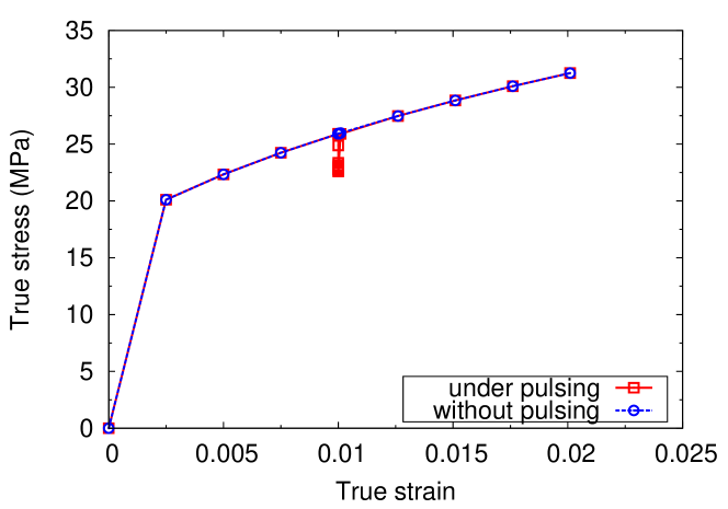
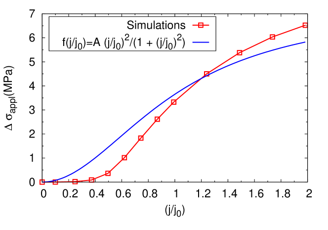
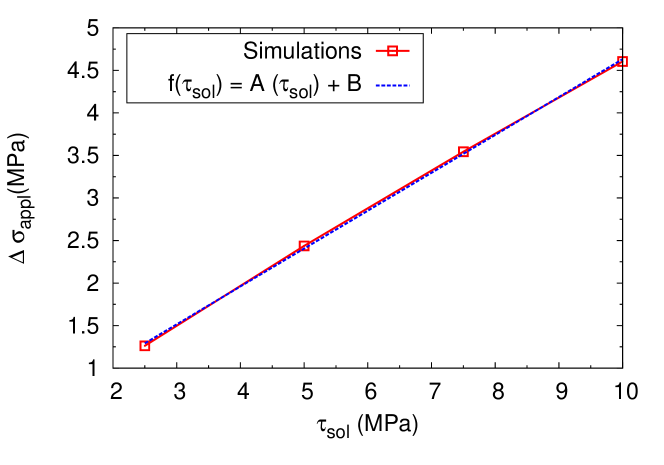
Figure 1: Figures demonstrating different aspects of the reductions in flow stress due to a change in $\tau_{sol}$. (a) Flow curves with and without electropulsing during a compression test. The imposed strain rate is $\dot{\epsilon}=1e-03\text{s}^{-1}$ and the pulse is applied at a strain of $0.01$. The imposed pulse corresponds to $j/j_{0}\approx 1$ and is applied for a total time of $60\,\mu\text{s}$. (b) Reductions in flow stress as a function of $(j/j_{0})$. (c) reductions in flow stress as a function of $\tau_{sol}$ at $j=j_{0}$. The constants A and B in the figure legends are determined by fitting to the simulation data. For (b) and (c) the loading and pulsing details are the same as in (a).

Moving on to the second possible source of reductions in flow stress which is an increase in $\lambda_{slip}^{\alpha}$, the corresponding flow curve in Fig. 2 hardly shows a difference from the un-pulsed one. A slight rise in the flow stress of $\approx 1e-06\,\text{MPa}$ can be discerned when we magnify the flow curves around the strain at which the pulse has been applied as seen in Fig. 2. A rise in flow stress during electropulsing is consistently observed for this particular mechanism across the entire range of $(j/j_{0})$ considered in Fig. 1. But as the increase in stresses are in the same range as the errors due to numerical discretization and precision, a clear trend does not emerge in the variation of $\Delta\sigma_{appl}$ versus $(j/j_{0})$, like observed in Fig. 1. The possibility of an increase of the flow stress instead of a drop when $\lambda_{slip}^{\alpha}$ increases has been discussed in Section 3.1.2.

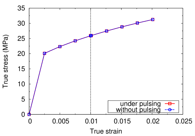
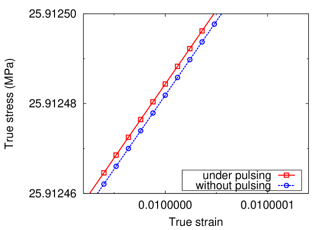
Figure 2: Figures demonstrating reductions in flow stress due to a change in $\lambda_{slip}^{\alpha}$. (a) Flow curves with and without electropulsing during a compression test. (b) The magnified version of (a) around a true strain of $0.01$. The loading and pulsing details are mentioned in the caption to Fig. 1.

We now consider the effects of a change in $v_{0}$ on the flow curve. A flow curve for this situation is no longer presented as it resembles Fig. 2 and instead we just present a variation of the reductions in flow stress as a function of $(j/j_{0})$ in Fig. 3. It is clear that the reductions in flow stress due to a change in $v_{0}$ are about two orders of magnitude lower than those observed for the case where a change in $\tau_{sol}$ is the source of softening. Also, the reductions in flow stress appear to be a parabolic function of $(j/j_{0})$ and do not display a good fit with an expression of the form predicted by Eq. 33. The reasons for this deviation are the same as the ones mentioned during the discussion of the reductions in flow stress due to a change in $\tau_{sol}$.

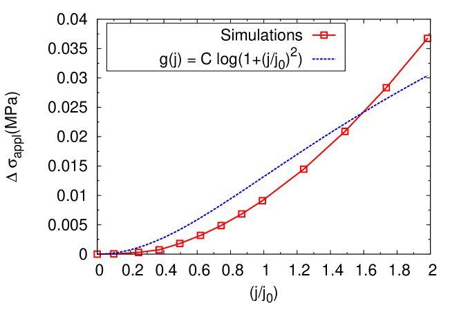
Figure 3: Figure demonstrating reductions in flow stress due to a change in $v_{0}$ as a function of $(j/j_{0})$. The loading and pulsing details are mentioned in the caption to Fig. 1. The constant $C$ is determined by fitting to the simulation data.

This brings us to the final source of change when dislocations are de-pinned from obstacles, reflected by a change in $\tau_{pass}^{\alpha}$. The value of the parameter $\beta$ in Eq. 38 is chosen to be of the same order of magnitude as that reported in [31](see Table. 2). As discussed earlier, when de-pinned, larger free length of dislocations respond strongly to the elastic stress fields due to other dislocations which lead to larger strain hardening. Thus, this is a mechanism which always leads to an increase in flow stress during pulsing as confirmed from Fig. 4 where the reductions in flow stress are presented as functions of $(j/j_{0})$. The nature of the curve is parabolic and hence allows a close fit by a function $f(j/j_{0})=A(j/j_{0})^{2}$ following Eq. 38 where $A$ is a fitting constant. The close fit between the form of Eq. 38 and those observed in Fig. 4 is rather fortuitous given the assumptions of the analytical predictions. The maximum value of the rise in $\Delta\sigma_{appl}$ over the range of current densities considered is insignificant compared to a drop caused by a change in $\tau_{sol}$.

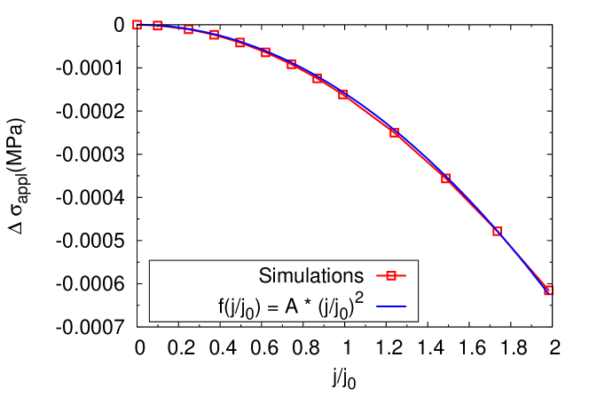
Figure 4: Figure demonstrating stress rises due to a change in $\tau_{pass}^{\alpha}$ as a function of $(j/j_{0})$. The loading and pulsing details are mentioned in the caption to Fig. 1.

After dealing with the softening sources which are due to the de-pinning of dislocations from obstacles during electropulsing, we now focus on the effects of electron-wind force on dislocations. The variation of the reductions in flow stress due to electron-wind force $\Delta\sigma_{appl}$ as a function of $j$ has a parabolic character initially but displays a sharper change at higher values of $j$ as evident from the last three points of the curve presented in Fig. 5. Such a behaviour correlates well with the nature of the ’$\cosh$’ function which is introduced as a factor in Eq. 44. As claimed by Molotskii et al., [13], we see a very small stress drop of the order of $1e-03\,\text{MPa}$ due to this mechanism. The selection of the relevant parameters like $\rho_{D}/N_{D}$ and $n_{e}$ which control the softening through this particular mechanism is described in the Appendix and their values are presented in Table 2.

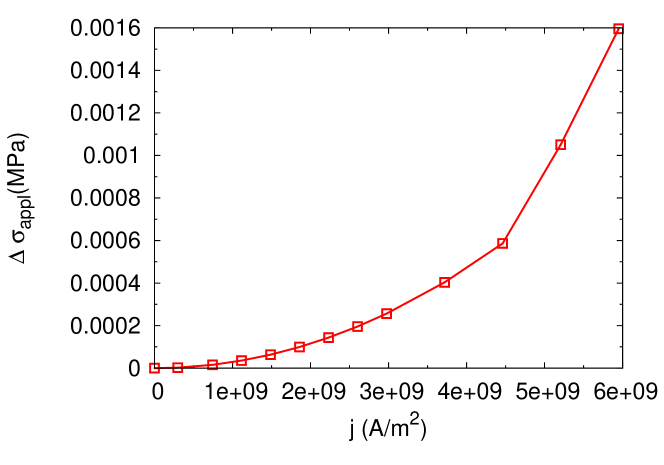
Figure 5: Figure demonstrating the reductions in flow stress due to electron-wind force as a function of $j$. The loading and pulsing details are mentioned in the caption to Fig. 1.

Through the results presented so far, we have developed an understanding of the nature and magnitude of the reductions in flow stress due to the de-pinning of dislocations and the electron-wind force. These mechanisms induce some changes either in the interaction between dislocations and obstacles or modify the forces acting on dislocations. In other words, these mechanisms do not invoke a change in temperature of the material and hence are athermal in character. It is important to determine the quantum of the reduction in flow stress achievable due to Joule heating of the material and compare it against the softening observed from athermal means. The first result in this regard is a variation of temperature rise ($\Delta T$) with $j$ as presented in Fig. 6. The corresponding reductions in flow stress are presented in Fig. 6. The variation of temperature rise with $j$ follows a parabolic curve which is in accordance with our analysis expressed by Eq. 52. The nature of the curve in Fig. 6 is parabolic for $j>2e09\,\text{A/m}^{2}$ and is in accordance with that predicted by Eq. 6. For $j<2e09\,\text{A/m}^{2}$, the softening response seen in simulations is lower than that predicted by our analysis. Such values of $j$ correspond to low temperature rises of $\Delta T<5\text{K}$, which can be conjectured to be not large enough to cause significant lowering of flow stress due to enhanced thermal activation. In other words, it appears, that unless the temperature exceeds a certain threshold value, there is no significant softening due to Joule-heating. This brings the limitation of analytical expressions like Eq. 6 again to the forefront as the assumptions involved in deriving such expressions are too simplistic compared to actual crystal plasticity simulations. The reductions in flow stress $\Delta\sigma_{appl}$ observed due to Joule-heating are higher than all the other softening sources discussed above except for the case where a change in $\tau_{sol}$ causes softening. It can be noted that the activation energies for slip ($Q_{s}$) and climb ($Q_{c}$) are the key parameters which control the reductions in flow stress due to Joule-heating. We have described the process of selection of $Q_{s}$ in the Appendix, and from Fig. 6 it is reasonable to argue that the rise in temperature is not enough to cause significant climb of edge dislocations.

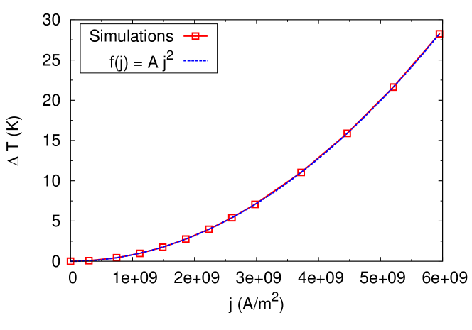
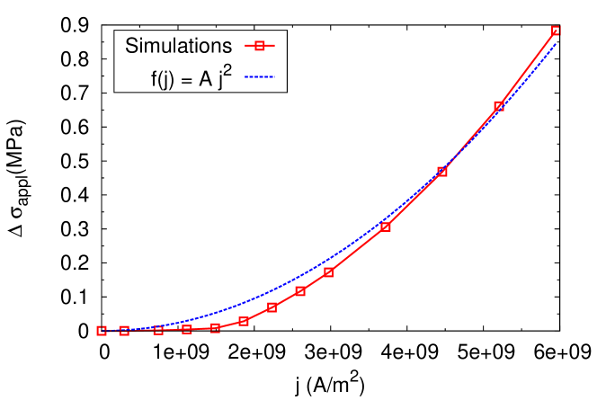
Figure 6: Figures demonstrating the reductions in flow stress due to Joule-heating. (a) Temperature rise as a function of $j$. (b) Reductions in flow stress as a function of $j$. The parameter $A$ in the figure legends denote constants which have to be determined by fitting to simulation data. The loading and pulsing details are mentioned in the caption to Fig. 1.

We have presented and discussed all the mechanisms and their corresponding sources which result in the electroplastic effect. A graphical summary of our observations is presented in Fig. 7 where the $\%$ drops in stress are plotted as function of the current density $j$. These figures unambiguously point to modifications in $\tau_{sol}$ being the strongest contributor to the reductions in flow stress. Thermal softening due to joule heating is a distant second, while all the other mechanisms produce reductions in flow stress which are at least smaller by an order of magnitude compared to Joule-heating. A curve obtained from a simulation where all the effects are simultaneously active (denoted by a legend “All” in the figure) lies in close proximity to the $\tau_{sol}$ curve and mimics its shape confirming changes in $\tau_{sol}$ to be the largest contributor to the reductions in flow stress.

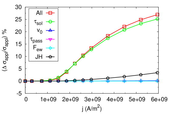
Figure 7: Figure comparing the $\%$ reductions in flow stress due to all the mechanisms, plotted as a function of $j$. In the figure legends, JH denotes Joule-heating, $F_{ew}$ denotes electron-wind force, and ’All’ refers to all mechanisms of EP being active. $\tau_{sol}$ and $v_{0}$ represent reductions in flow stress due to changes in those terms.

There is a considerable experimental evidence that the magnitudes of the reductions in flow stress are reduced as the the pulses are applied at higher values of strains [5, 10, 14]. In Figs. 8 and 8, we present a variation of the reductions in flow stress due to a change in $\tau_{sol}$ and Joule-heating respectively, as functions of the strains at which the sample is pulsed. It can be seen from Fig. 8 that $\Delta\sigma_{appl}$ falls as pulses are applied at higher strains. This could be explained in the following manner. In our crystal plasticity framework, higher strains are microstructurally characterized by a larger value of $\rho_{m}^{\alpha}$ (and also $\rho_{d}^{\alpha})$. Invoking the assumption that an imposed $\dot{\epsilon}$ leads to constant values of $\dot{\gamma^{\alpha}}$ on the different slip planes $\alpha$, from Eq. 7 it is clear that for larger values of $\rho_{m}^{\alpha}$ at higher strains, smaller values of $\tau_{eff}^{\alpha}$ satisfy Eq. 7. As $\sigma_{eff}$ is related to $\tau_{eff}^{\alpha}$ by a Taylor factor, the value of $\sigma_{eff}$ will also be lowered as the strains increase. The direct proportionality between the reductions in flow stress ($\Delta\sigma_{appl}$) due to a change in $\tau_{sol}$ and $\sigma_{eff}$ due to Eq. 25 explains the lowered reductions in flow stress ($\Delta\sigma_{appl}$) at higher values of strains. In other words, at higher levels of strains, plasticity is achieved by generating more mobile dislocations to compensate for the smaller dislocation free paths. Thus, at higher strains, the mechanisms of EP which aid thermal activation of the dislocation segments over short range obstacles can only enhance the much lower dislocation velocity by a smaller factor, compared to that possible at smaller strains.

In contrary to our observations in Fig. 8, the reductions in flow stress due to thermal softening increase with applied strains as shown in Fig. 8. Using the concept of the reduction in $\sigma_{eff}$ with strain as described in the previous paragraph, the increase in reductions in flow stress observed in Fig. 8 could be immediately explained from Eq. 54. But as these changes are an order of magnitude smaller than those observed in Fig. 8, the curve corresponding to the case where all the softening mechanisms are operative, mimics the one representing reductions in flow stress due to a change in $\tau_{sol}$ (see Fig. 8). The influence of the other mechanisms of EP are not considered to be important because they have been seen to produce a negligibly small impact on the reductions in flow stress.

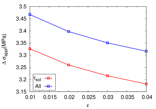
Figure 8: Figures demonstrating the reductions in flow stress ($\Delta\sigma_{appl}$) due to, (a) a change in $\tau_{sol}$ and when all the mechanisms are active, and (b) Joule-heating, with strains ($\epsilon$) at which electrical pulses are applied. The figure legends are explained in the caption to Fig. 7. Pulses of magnitude $3e09\,\text{A/m}^{2}$ are applied for a total time of $60\,\mu\text{s}$.

Finally, we probe the effect of pulse duration on the reductions in flow stress as presented in Fig. 9, where the pulse duration is increased keeping the current density constant. The reductions in flow stress due to a change in $\tau_{sol}$ increase gradually as the pulse durations are increased and show signs of saturation at higher pulse durations. This can be explained by discretizing the entire pulse duration into a series of infinitesimal pulses, each lowering the $\sigma_{eff}$ to a value which becomes the initial $\sigma_{eff}$ for the subsequent pulse (see Eq. 24). Noting that $\sigma_{eff}<<\sigma_{appl}$ and $(\sigma_{eff}/M)<\tau_{sol}$, the proportionality of $\Delta\sigma_{appl}$ with $\sigma_{eff}$ (see Eq. 25) means that the reductions in flow stress increase with the pulse size, but ultimately saturates. Thermal softening due to Joule heating is strongly affected as more electrical energy is introduced into the material as the pulse duration increases. Joule heating being the mechanism which is most sensitive to an increase in pulse duration dominates the overall sensitivity of the electroplastic effect even when all the mechanisms are active as seen in Fig. 9.

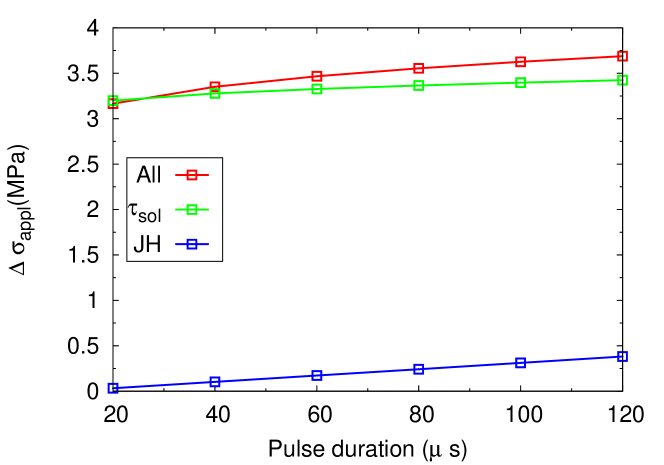
Figure 9: Figure demonstrating the variation of the reductions in flow stress as a function of the pulse width. The current density is maintained at $j=3e09\,\text{A/m}^{2}$. The figure legends are explained in the caption to Fig. 7.

Having reached the end of this section, we will summarize our key observations:

• De-pinning of dislocations produces the largest reductions in flow stress through a change in $\tau_{sol}$.

• Joule-heating is the second largest contributor to the reductions in flow stress but its contribution is still an order of magnitude smaller than that produced by dislocation de-pinning.

• Electron-wind force has negligible contribution to the reductions in flow stress.

• The reductions in flow stress due to de-pinning of dislocations fall as the electrical pulses are applied at higher strains.

• Increasing duration of the electrical pulses increases the reductions in flow stress due to both Joule-heating and dislocation de-pinning.

• As the reductions in flow stress due to de-pinning of dislocations are a strong function of $\tau_{sol}$, it can be expected that for certain combinations of parameters, Joule-heating produces larger reductions in flow stress than that due to de-pinning of dislocations.

In the next section, we discuss a few implications of our results and lay out the possibilities for future work in this direction.

6 Discussion

As already discussed, for the parameter set considered, dislocation de-pinning produces a reduction in flow stress which is an order of magnitude larger than that produced by Joule-heating. But our simulations also demonstrate that it is possible for Joule-heating to supersede the de-pinning of dislocations as the dominant mechanism of EP. This happens when the temperature rise produced in the material is large enough to cause a softening higher than the softening produced by de-pinning of dislocations. In context of this understanding, a few experimental evidences which claim EP to be predominantly a Joule-heating phenomenon can now for the first time be explained consistently within the framework of our model. Examples of such studies are due to Magargee et al., [12] and Zheng et al., [36]. It must be noted that the material under consideration in these studies is Ti, which has a hexagonal close packed structure. The fact that there are not enough slip systems in a hexagonal structure to produce a predominantly dislocation mediated plasticity also implies that dislocations interact with forest dislocations much rarely in such materials resulting in smaller values of $\tau_{sol}$, compared to those observed for FCC materials. Hence, it is possible that for such materials, de-pinning of dislocations during electropulsing may not be the dominant softening mechanism. This point has also been raised by Sprecher et al., [5] where they claim that the interstitial impurities in Ti present the largest barriers to dislocation motion for hexagonal metals. So, for such a material it is quite reasonable that thermal softening due to Joule-heating is the dominant mechanism for EP, especially when the interstitial solutes are not paramagnetic in character. Another work by Goldman et al., [11] reports no softening in Pb at superconducting temperatures (around $4K$). This could be explained by considering that a change in electronic behaviour which induces superconductivity at low temperatures could also potentially inhibit the mechanism of de-pinning of dislocations, which is dependent on electronic states.

With reference to the discussion in the previous paragraph, it can be noted that while the mechanism of de-pinning of dislocations is of central importance to the phenomenon of EP in FCC materials and may be of significance for Hexagonal materials as well, this is not valid for BCC materials, as has already been pointed out by Molotskii [14]. For BCC materials, slip is largely determined by the well known kink-pair mechanism, and the way that mechanism is affected by electropulsing continues to remain unclear. Hence some experimental suggestions are crucial to formulate an athermal theory of EP for BCC materials.

7 Acknowledgement

The authors gratefully acknowledge the financial support by the DFG Priority Programme SPP 1959/1, ”Manipulation of matter controlled by electric and magnetic field: Toward novel synthesis and processing routes of inorganic materials” with the grant number of 319419837.

8 Appendix

Here, we present a short description of the process of selection of different parameters which influence the reductions in flow stress during electropulsing. We first describe selection of $\tau_{sol}$ which is central to the reductions in flow stress observed due to dislocation de-pinning. The parameters critical to electron-wind force $\rho_{D}/n_{d}$ and $n_{e}$ are discussed next.

8.1 Selection of $Q_{s}$ and $\tau_{sol}$

The activation energy for slip $Q_{s}$ is related to the energy of forming a jog as a dislocation intersects a forest dislocation. This energy has been estimated to be between $Gb_{s}^{3}/5$ and $Gb_{s}^{3}/3$ [37] and we assume it to be,

$$Q_{s}=\dfrac{1}{4}Gb_{s}^{3}.$$ (56)

For fcc materials, it is often seen that $Gb_{s}^{3}\approx 4\text{eV}$ [37], hence $Q_{s}=1eV=1.6e{-}19\text{J}$ from Eq. 56. When a jog is created by an applied stress $\tau^{*}$ we can write,

$$Q_{s}=\tau^{*}V,$$ (57)

where $V$ is the activation volume defined as,

$$V=b_{s}d_{ac}l_{c},$$ (58)

with $d_{ac}$ and $l_{c}$ denote the activation distance and average free dislocation segment length, respectively. For jog formation during forest dislocation interaction, $d_{ac}\approx b_{s}$ [37], and $l_{c}\approx 1000b_{s}$ [38]. Assuming $b_{s}=2.86e{-}10\,\text{m}$, using Eqs. 57 and 58, we get, $V\approx 1000b_{s}^{3}$ and $\tau^{*}\approx 7\,\text{MPa}$. Conceptually, $\tau^{*}$ is the same as $\tau_{sol}$ as the latter represents the stress required for dislocations to overcome short range obstacles like forest dislocations. This exercise allows us to identify two important parameters for our crystal plasticity simulations: $\tau_{sol}=7\,\text{MPa}$ and $Q_{s}=1.6e{-}19\,\text{J}$.

8.2 The parameters influencing the electron-wind force

The two key parameters which affect the electron-wind force are the specific dislocation resistivity $\rho_{D}/N_{D}$ and the free electron density $n_{e}$. For the former, we use the value stated for Aluminium in  [39] while we compute $n_{e}$ using the formula,

$$n_{e}=\dfrac{fN_{A}\rho}{M_{A}},$$ (59)

where, $M_{A}$ is the atomic mass, $f$ is the number of free electrons per atom, $N_{A}$ is the Avogadro number and $\rho$ is the density. We compute $n_{e}$ using the parameters for Aluminium.

References

- Troitskii and Likhtman [1963] O. Troitskii, V. Likhtman, The effect of the anisotropy of electron and radiation on the deformation of zinc single crystals in the brittle state, Kokl. Akad. Nauk. SSSR 148 (1963) 332.
- Roth et al. [2008] J. T. Roth, I. Loker, D. Mauck, M. Warner, S. F. Golovashchenko, A. Krause, Enhanced formability of 5754 aluminum sheet metal using electric pulsing, in: Transactions of the North American Manufacturing Research Institution of SME, 405–412, 2008.
- Salandro et al. [2009] W. A. Salandro, A. Khalifa, J. T. Roth, Tensile formability enhancement of magnesium AZ31B-0 alloy using electrical pulsing, in: 37th Annual North American Manufacturing Research Conference, NAMRC 37, 387–394, 2009.
- Salandro et al. [2010] W. A. Salandro, J. J. Jones, T. A. McNeal, J. T. Roth, S.-T. Hong, M. T. Smith, Formability of Al 5xxx sheet metals using pulsed current for various heat treatments, Journal of manufacturing science and engineering 132 (5) (2010) 051016.
- Sprecher et al. [1986] A. Sprecher, S. Mannan, H. Conrad, Overview no. 49: On the mechanisms for the electroplastic effect in metals, Acta Metallurgica 34 (7) (1986) 1145–1162.
- Guan et al. [2010] L. Guan, G. Tang, P. K. Chu, Recent advances and challenges in electroplastic manufacturing processing of metals, Journal of Materials Research 25 (7) (2010) 1215–1224.
- Nguyen-Tran et al. [2015] H.-D. Nguyen-Tran, H.-S. Oh, S.-T. Hong, H. N. Han, J. Cao, S.-H. Ahn, D.-M. Chun, A review of electrically-assisted manufacturing, International Journal of Precision Engineering and Manufacturing-Green Technology 2 (4) (2015) 365–376.
- Ruszkiewicz et al. [2017] B. J. Ruszkiewicz, T. Grimm, I. Ragai, L. Mears, J. T. Roth, A review of electrically-assisted manufacturing with emphasis on modeling and understanding of the electroplastic effect, Journal of Manufacturing Science and Engineering 139 (11) (2017) 110801.
- Conrad et al. [1990] H. Conrad, A. F. Sprecher, W. D. Cao, X. P. Lu, Electroplasticity—the effect of electricity on the mechanical properties of metals, JOM 42 (9) (1990) 28–33.
- Conrad [2002] H. Conrad, Thermally activated plastic flow of metals and ceramics with an electric field or current, Materials Science and Engineering: A 322 (1-2) (2002) 100–107.
- Goldman et al. [1981] P. Goldman, L. Motowidlo, J. Galligan, The absence of an electroplastic effect in lead at 4.2 K, Scripta Metallurgica 15 (4) (1981) 353–356.
- Magargee et al. [2013] J. Magargee, F. Morestin, J. Cao, Characterization of flow stress for commercially pure titanium subjected to electrically assisted deformation, Journal of Engineering Materials and Technology 135 (4) (2013) 041003.