Fronts in two-phase porous flow problems: effects of hysteresis and dynamic capillarity

Abstract

In this work, we study the behaviour of saturation fronts for two phase flow through a long homogeneous porous column. In particular, the model includes hysteresis and dynamic effects in the capillary pressure and hysteresis in the permeabilities. The analysis uses travelling wave approximation. Entropy solutions are derived for Riemann problems that are arising in this context. These solutions belong to a much broader class compared to the standard Oleinik solutions, where hysteresis and dynamic effects are neglected. The relevant cases are examined and the corresponding solutions are categorized. They include non-monotone profiles, multiple shocks and self-developing stable saturation plateaus. Numerical results are presented that illustrate the mathematical analysis. Finally, we compare experimental results with our theoretical findings.

1 Introduction

Modelling of two phase flow through the subsurface is important for many practical applications, from groundwater modelling and oil and gas recovery to CO₂ sequestration. For this purpose the mass balance equations are used which read in the absence of source terms [2, 30] as follows:

$$\phi\frac{\partial\left(\rho_{\alpha}S_{\alpha}\right)}{\partial t}+\nabla\cdot\left(\rho_{\alpha}v_{\alpha}\right)=0,\;\alpha\in\left\{w,n\right\},$$ (1)

where $\alpha=n$ denotes the non-wetting phase and $\alpha=w$ the wetting phase. Further, $\phi$ is the porosity, $S_{\alpha}$ and $\rho_{\alpha}$ the saturation and density of the phases. The phase-velocities $v_{\alpha}$ are given by the Darcy’s law [2, 30],

$$v_{\alpha}=-\frac{k_{r\alpha}}{\mu_{\alpha}}K\left(\nabla p_{\alpha}-\rho_{\alpha}g\hat{e}_{g}\right),\;\alpha\in\left\{w,n\right\}.$$ (2)

Here $K\left[\mathrm{m}^{2}\right]$ is the absolute permeability of the porous medium, $\mu_{\alpha}\left[Pa\cdot s\right]$ the viscosity and $k_{r\alpha}$ the relative permeability of each phase. Moreover, $p_{\alpha}\;\left[\mathrm{Pa}\right]$, $g\;\left[\nicefrac{\mathrm{m}}{\mathrm{s^{2}}}\right]$ and $\hat{e}_{g}$ stand for the phase pressure, the gravitational acceleration and the unit vector along gravity, respectively. Observe that the system (1)-(2) is not closed as there are more unknowns than equations, i.e. $S_{\alpha}$, $k_{r\alpha}$ and $p_{\alpha}$. Hence, one needs to take certain assumptions. Assuming incompressibility results in $\rho_{\alpha}$ being constant. Moreover, by definition

$$S_{w}+S_{n}=1.$$ (3)

Commonly it is assumed that the relative permeabilities, as well as the phase pressure difference, are functions of the saturation of the wetting phase [2, 30],

$$k_{rn}=k_{rn}(S_{w}),\quad k_{rw}=k_{rw}(S_{w})\text{ and }p_{n}-p_{w}=p_{c}(S_{w}).$$ (4)

The function $p_{c}:(0,1]\to\mathbb{R}^{+}$ is referred to as the capillary pressure function. System (1)-(4) reduces to the hyperbolic Buckley-Leverett equation if this term is neglected, i.e. $p_{c}\equiv 0$. The model given by (1)-(4) works well under close to equilibrium conditions and when flow reversal does not take place. However, some more general cases cannot be explained by this model.

One of the first evidences of deviation from the standard model was reported in the 1931 paper by Richards [57] where he concluded that the capillary pressure term is hysteretic in nature. Capillary hysteresis refers to the phenomenon that $p_{c}$ measured for a wetting phase infiltration process follows a curve, denoted here by ${p^{(i)}_{c}}(S_{w})$, which differs from $p_{c}$ measured for a drainage process, denoted by ${p^{(d)}_{c}}(S_{w})$. If the process changes from infiltration to drainage or vice versa, then the $p_{c}$ follows scanning curves that are intermediate to ${p^{(i)}_{c}}(S_{w})$ and ${p^{(d)}_{c}}(S_{w})$ [6]. This is shown in detail in Figure 1 (left). Since then, hysteresis has been studied experimentally [44, 54, 73], analytically [15, 68, 5, 62, 55] and numerically [71, 48, 55, 59, 10]. Variety of models have been proposed to incorporate the effects of hysteresis, such as independent and dependent domain models [50, 45, 49] and interfacial area models [27, 29, 53, 46]. A comprehensive study of these models can be found in [20]. However, in this paper we will use the play-type hysteresis model [6, 20] that approximates scanning curves as constant saturation lines. This model is comparatively simple to treat analytically [15, 62, 55, 68], it has a physical basis [6, 60] and it can be extended to depict the realistic cases accurately [20].

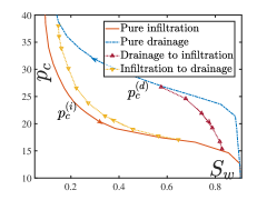
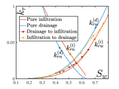
Figure 1: (left) Hysteresis of capillary pressure and scanning curves. The plots drawn use data points from Figure 4 and 5 of [44]. (right) Hysteresis of relative permeabilities. Experimental data from [66] are used for t he $k_{rw}$ plots and the corresponding scanning curves. Plots for $k_{rn}$ show data from [24]. The curves are scaled in the $y$ direction.

A similar hysteretic behaviour is observed for the relative permeabilities too, although to a lesser extent. Hysteresis of the non-wetting phase relative permeability in the two phase case (oil and water for example) is reported in [24, 9, 36]. The wetting permeability $k_{rw}$ also exhibits hysteresis [66, 54] but the effect is less pronounced, see Figure 1 (right).

Another effect that cannot be explained by the standard model is the occurrences of overshoots. More precisely, in infiltration experiments through initially low saturated soils it is observed that if the flow rate is large enough then the saturation at an interior point is larger than that on the boundary even in the absence of internal sources [19, 8, 64]. This cannot be explained by a second order model such as (1)-(4) [21, 70, 61]. Hence, based on thermodynamic considerations the dynamic capillary model was proposed in [28]. Since then the dynamic capillary term has been measured experimentally [12, 33] and it was used successfully to explain overshoots [18, 69, 67, 68, 43, 55, 62]. Also the well-posedness of the dynamic capillarity model has been proved [17, 16, 41, 7] and numerical methods have been investigated [34, 14, 35, 13, 23].

Figure 2: Setup of an infiltration experiment. At the inlet of a column having the height $H$ water is injected by a constant rate. The main axis of the column is orientated such that it is aligned with the gravity vector.

In this paper we are interested in studying how the flow behaviour is influenced if one considers the non-equilibrium effects, i.e. hysteresis and dynamic capillarity. For this purpose, we study the system in a one-dimensional setting. The one dimensional case is relevant when one spatial direction is dominant; it approximates flow through viscous fingers [55, 25, 56] and it can explain results from the standard experimental setting shown in Figure 2 [19, 8, 64]. In this study, the behaviour of the fronts is investigated by traveling wave (TW) solutions. The TW solutions can approximate the saturation and pressure profiles in an infiltration experiments through a long column, and the existence conditions of the TWs act as the entropy conditions for the corresponding hyperbolic model when the viscous terms are disregarded. For the unsaturated case ($p_{n}=0$) TW solutions with dynamic effect were analysed in [18]. For the two phase case it was shown rigorously in [69, 67, 65] that non-monotone travelling waves and non-standard entropy solutions are existing if one includes dynamic capillarity effect. Similar analysis but for higher order viscous terms containing spatial derivatives were performed in [3, 22]. The existence of TW solutions for the unsaturated case when dynamic capillarity and capillary hysteresis are present was proved in [68, 43] and criteria for non-monotonicity and reaching full saturation were stated. It is evidenced in [59, 31] that hysteresis can explain stable saturation plateaus but it cannot initiate them. In [55, 5] it is shown how both hysteresis and dynamic capillarity are required to explain the growth of viscous fingers. The entropy conditions for Buckley-Leverett equation considering hysteresis in only permeability were derived in [51, 58, 4]. However, hysteresis and nonlinearities were not included in the viscous term. This is taken into consideration in [1] where the authors add a dynamic term to model permeability hysteresis, while disregarding hysteresis and dynamic effects in capillary pressure. The behaviour of TW for a non-monotone flux function in the presence of a third order term was described in [63].

In our current work we build upon [18, 69, 67, 68, 43] to describe the behaviour of fronts in the two-phase case when dynamic capillarity and both type of hysteresis are included. The models that are used in our analysis are introduced in Section 2. Section 3 discusses the existence of TWs when hysteresis and dynamic effects are included in the capillary pressure but not in the permeabilities. Entropy conditions are derived and they reveal that there can be non-classical shocks. In Section 4, the analysis is extended to include hysteresis in the permeabilities. This makes self-developing stable saturation plateaus and a broader class of entropy solutions possible. Section 5 presents numerical results that support our analytical findings. Finally, we make some concluding remarks in Section 6 and compare the results with experiments.

2 Mathematical model

This section is dedicated to the formulation of a mathematical model that can be used to describe an infiltration process of a fluid into a homogeneous porous column. An example for such an infiltration process is the injection of water into a dry sand column (see Figure 2).

2.1 Governing equations

Here we consider the one-dimensional situation where the flow problem is defined on an interval $\left(0,H\right)$. This simplification is justified by the fact that the walls of the porous column, in which the fluids are injected are impermeable and that saturation is in general almost constant across the section area of the column. The axis is pointing in the direction of gravity. The medium is assumed to be homogeneous and the fluids are incompressible. Under these constraints, (1)-(2) simplify to

$$\phi\frac{\partial S_{\alpha}}{\partial t}+\dfrac{\partial v_{\alpha}}{\partial z}=0,\;v_{\alpha}=-\dfrac{k_{r\alpha}}{\mu_{\alpha}}K\left(\dfrac{\partial p_{\alpha}}{\partial z}-\rho_{\alpha}g\right),\;\alpha\in\left\{w,n\right\},$$ (5)

where $t$ and $z$ are denoting the time and space variables, respectively. To further simplify the model, after summing (5) for the two phases and using (3) we observe that the total velocity

$$v(z,t)=v_{w}(z,t)+v_{n}(z,t)$$ (6)

is constant in space. In addition to that, we assume that $v$ is also constant in time, which occurs, e.g. if a constant influx (injection rate) is prescribed at the inlet $z=0$. This gives

$$\frac{\partial v}{\partial t}=\frac{\partial v}{\partial z}=0,\text{ or }v\left(z,t\right)\equiv v\text{ for }z\in(0,H)\text{ and }t>0.$$ (7)

From (5)-(7) one finds

$$v_{w}=\frac{k_{rw}}{k_{rw}+\frac{\mu_{w}}{\mu_{n}}k_{rn}}v+\dfrac{K}{\mu_{n}}\frac{k_{rw}k_{rn}}{k_{rw}+\frac{\mu_{w}}{\mu_{n}}k_{rn}}\left(\frac{\partial p_{c}}{\partial z}+\left(\rho_{w}-\rho_{n}\right)g\right).$$ (8)

At this stage we define the fractional flow function

$$f:=\frac{k_{rw}}{k_{rw}+\frac{\mu_{w}}{\mu_{n}}k_{rn}},$$ (9)

and the function

$$h:=\frac{k_{rw}k_{rn}}{k_{rw}+\frac{\mu_{w}}{\mu_{n}}k_{rn}}=k_{rn}f.$$ (10)

Substituting these relations and definitions into (5) for $\alpha=w$ yields the transport equation for the wetting phase

$$\frac{\partial S}{\partial t}+\frac{v}{\phi}\frac{\partial}{\partial z}\left[f+\frac{K\left(\rho_{w}-\rho_{n}\right)g}{v\mu_{n}}h+\frac{K}{v\mu_{n}}h\frac{\partial p}{\partial z}\right]=0,$$ (11)

where we used the notation

$$S:=S_{w}\text{ and }p:=p_{n}-p_{w}.$$ (12)

Note that, $f$ and $h$ are functions of $S$ and possibly of $p$, as shown below.

2.2 Modelling hysteresis and dynamic capillarity

To incorporate hysteresis and dynamic capillarity in the model, one needs to extend capillary pressure and relative permeability given in the closure relationship (4).

2.2.1 Capillary pressure

The following expression is used to extend the capillary pressure:

$$p\in\frac{1}{2}({p^{(i)}_{c}}(S)+{p^{(d)}_{c}}(S))-\frac{1}{2}({p^{(d)}_{c}}(S)-{p^{(i)}_{c}}(S))\cdot{\rm sign}\left(\frac{\partial S}{\partial t}\right)-\tau\frac{\partial S}{\partial t},$$ (13)

where $\text{sign}(\cdot)$ denotes the multi-valued signum graph

$$\text{sign}\left(\xi\right)=\begin{cases}1,&\text{ for }\xi>0,\\ \left[-1,1\right],&\text{ for }\xi=0,\\ -1,&\text{ for }\xi<0,\end{cases}$$ (14)

see [6, 28, 62]. The second and third term in the right hand side of (13) describe, respectively, capillary hysteresis [6] and dynamic capillarity [28]. Further, $\tau\geq 0$ denotes the dynamic capillary coefficient. It models relaxation or damping in the capillary pressure. Although in practice $\tau$ may depend on $S$ [12, 8], here we assume it to be constant. The case of non-constant $\tau$ is considered in [68, 43]. The capillary pressure functions $p_{c}^{\left(j\right)}$, $j\in\{i,d\}$, fulfill [2, 30, 44]:

1. $p_{c}^{\left(j\right)}:\left(0,1\right]\rightarrow\left[0,\infty\right),\;p_{c}^{\left(j\right)}\in C^{1}\left(\left(0,1\right]\right),\;p_{c}^{\left(j\right)}\left(1\right)=0.$ Moreover, ${p_{c}^{\left(j\right)}}^{\prime}\left(S\right)<0\text{ and }p_{c}^{\left(i\right)}\left(S\right)<p_{c}^{\left(d\right)}\left(S\right)\text{ for }S\in\left(0,1\right).$

Here, and later in this paper, a prime denotes differentiation with respect to the argument. In the absence of dynamic effects, i.e. $\tau=0$, expression (13) implies

$$p=\begin{cases}{p^{(i)}_{c}}(S)&\text{ when }\partial_{t}S>0,\\ {p^{(d)}_{c}}(S)&\text{ when }\partial_{t}S<0.\end{cases}$$

This is precisely what is seen from water infiltration/drainage experiments [44]. When $\frac{\partial S}{\partial t}=0$, $p$ is between ${p^{(i)}_{c}}(S)$ and ${p^{(d)}_{c}}(S)$. For this reason, the hysteresis described by (13) is called play-type hysteresis: i.e. the scanning curves between ${p^{(i)}_{c}}(S)$ and ${p^{(d)}_{c}}(S)$ are vertical.

Before discussing the case $\tau>0$, we introduce for convenience the sets

$${\mathcal{H}^{(i)}}:=\{(S,p):S\in(0,1],\;p<{p^{(i)}_{c}}(S)\},$$ (15)

$${\mathcal{H}^{(d)}}:=\{(S,p):S\in(0,1],\;p>{p^{(d)}_{c}}(S)\},$$ (16)

$${\cal H}:=\{(S,p):S\in(0,1],\;{p^{(i)}_{c}}(S)\leq p\leq{p^{(d)}_{c}}(S)\},$$ (17)

and the strip $\mathcal{W}={\mathcal{H}^{(i)}}\cup{\cal H}\cup{\mathcal{H}^{(d)}}=\{0<S\leq 1\}$. In [43] it is shown that pressure expression (13) can be written as

$$\frac{\partial S}{\partial t}=\frac{1}{\tau}\mathcal{F}\left(S,p\right):=\frac{1}{\tau}\begin{cases}p_{c}^{(d)}\left(S\right)-p&\text{ if }(S,p)\in{\mathcal{H}^{(d)}},\\[-1.00006pt] 0&\text{ if }(S,p)\in{\cal H},\\[-1.00006pt] p_{c}^{(i)}\left(S\right)-p&\text{ if }(S,p)\in{\mathcal{H}^{(i)}}.\end{cases}$$ (18)

2.2.2 Relative permeability

To make the effect of hysteresis explicit in the relative permeabilities we need to incorporate a dependence on both $S$ and $\frac{\partial S}{\partial t}$. This dependence should satisfy

$$k_{r\alpha}\left(S,\frac{\partial S}{\partial t}\right)=\begin{cases}k^{(i)}_{r\alpha}\left(S\right)&\text{ if }\frac{\partial S}{\partial t}>0,\\ k^{(d)}_{r\alpha}\left(S\right)&\text{ if }\frac{\partial S}{\partial t}<0,\end{cases}\text{ for }\alpha\in\{w,n\}.$$ (19)

Here $k^{(i)}_{r\alpha},k^{(d)}_{r\alpha}:[0,1]\to\mathbb{R}$ are the infiltration and drainage relative permeabilities obtained from experiments [24, 9, 36, 66, 54]. In line with the experimental outcomes, we assume here for $j\in\{i,d\}$,

1. $k^{(j)}_{rw}\in C^{2}\left(\left[0,1\right]\right),\;{k^{(j)}_{rw}}^{\prime}\left(S\right)>0$ for $0<S\leq 1,\;k^{(j)}_{rw}\left(0\right)=0$ and $k^{(j)}_{rw}$ is strictly convex. Moreover, for $0<S<1$, $k^{(i)}_{rw}(S)<k^{(d)}_{rw}(S)$.

2. $k^{(j)}_{rn}\in C^{2}\left(\left[0,1\right]\right),\;{k^{(j)}_{rn}}^{\prime}\left(S\right)<0$ for $0\leq S<1,\;k^{(j)}_{rn}\left(1\right)=0$ and $k_{rn}$ is strictly convex. Moreover, for $0<S<1$, $k^{(d)}_{rn}(S)<k^{(i)}_{rn}(S)$.

Note the reverse ordering in $k_{rw}$ and $k_{rn}$ when switching from infiltration to drainage. This is demonstrated experimentally in [9, 24, 66], see also Figure 1.

In [72], a play-type approach has been proposed to model $k_{r\alpha}$ where

$$k_{r\alpha}\in\frac{1}{2}(k_{r\alpha}^{(d)}(S)+k_{r\alpha}^{(i)}(S))-\frac{1}{2}(k_{r\alpha}^{(d)}(S)-k_{r\alpha}^{(i)}(S))\cdot{\rm sign}\left(\frac{\partial S}{\partial t}\right).$$ (20)

However, this model is ill-posed in the unregularised case as for $\frac{\partial S}{\partial t}=0$ the relative permeabilities are undetermined, i.e. the relative permeabilities have no equation to determine them when $\frac{\partial S}{\partial t}=0$. This is different for the capillary pressure (13) because $p$ satisfies equation (11) as well. With the permeabilities we take an approach inspired by [51, 58, 4]. Here, inherited from the capillary pressure, the hysteresis is of the play-type as well, but now depending on $S$ and $p$, rather than on $S$ and $\frac{\partial S}{\partial t}$. We propose the following model: for $\alpha\in\{w,n\}$

$$k_{r\alpha}=k_{r\alpha}(S,p)=\begin{cases}k_{r\alpha}^{(d)}(S)&\text{ if }(S,p)\in{\mathcal{H}^{(d)}},\\ \bar{k}_{r\alpha}(S,p)&\text{ if }(S,p)\in{\cal H},\\ k_{r\alpha}^{(i)}(S)&\text{ if }(S,p)\in{\mathcal{H}^{(i)}}.\end{cases}$$ (21)

Here $\bar{k}_{r\alpha}:{\cal H}\to[0,\infty)$ is a given function that satisfies

1. $\bar{k}_{r\alpha}\in C^{2}({\cal H})$ such that $k_{r\alpha}\in C(\mathcal{W})$ for $\alpha\in\{w,n\}$ and $\partial_{p}\bar{k}_{rw}>0$, $\partial_{p}\bar{k}_{rn}<0$ in ${\cal H}$.

Observe that, this implies $\bar{k}_{r\alpha}(S,p^{(j)}_{c}(S))=k_{r\alpha}^{(j)}(S)$ for $j\in\{i,d\}$. For the moment we leave the choice of $\bar{k}_{r\alpha}$ unspecified, except for properties (P4), as it neither influences the entropy conditions nor the critical $\tau$ values introduced afterwards.

Remark 2.1.

In the computations one needs to specify an expression for $\bar{k}_{r\alpha}$. In Section 5 we use

$$\bar{k}_{r\alpha}(S,p)=k_{r\alpha}^{(i)}(S)+(k_{r\alpha}^{(d)}(S)-k_{r\alpha}^{(i)}(S))\left(\frac{p-{p^{(i)}_{c}}(S)}{{p^{(d)}_{c}}(S)-{p^{(i)}_{c}}(S)}\right).$$ (22)

This expression is obtained by considering ${\rm sign}$ in (13) and (20) as a function that can be eliminated. With $\tau=0$ in (13), this results in (22). Since the fraction (22) is bounded by 0 and 1 for $(S,p)\in{\cal H}$, we have $\lim_{S\searrow 0}k_{r\alpha}(S,p)=k_{r\alpha}^{(i)}(0)=k_{r\alpha}^{(d)}(0)$ and similar for $S\nearrow 1$.

Observe that (21) is consistent with (19) as from (18), $\frac{\partial S}{\partial t}>0$ iff $p<{p^{(i)}_{c}}(S)$ and $\frac{\partial S}{\partial t}<0$ iff $p>{p^{(d)}_{c}}(S)$. Moreover, the scanning curves for $k_{r\alpha}$ have constant $S$. Although not true in general, see for instance Figure 1, we restrict ourselves to play-type for both $p$ and $k_{r\alpha}$. An extension describing non-vertical scanning curves is discussed in [20].

Using (21) and (9),(10), the nonlinearities $f$ and $h$ are expressed in terms of $S$ and $p$ as well:

$$\zeta(S,p)=\begin{cases}\zeta^{(d)}(S)&\text{ if }(S,p)\in{\mathcal{H}^{(d)}},\\ \bar{\zeta}(S,p)&\text{ if }(S,p)\in{\cal H},\\ \zeta^{(i)}(S)&\text{ if }(S,p)\in{\mathcal{H}^{(i)}},\end{cases}\;\text{ for }\zeta\in\{f,h\}.$$ (23)

From (P2)-(P4) we deduce for $f$ and $h$:

1. $f\in C(\mathcal{W})$, $\bar{f}\in C^{2}({\cal H})$ and $\partial_{p}\bar{f}>0$ in ${\cal H}$. For $j\in\{i,d\}$, $f^{(j)}\in C^{2}\left(\left[0,1\right]\right)$, ${f^{(j)}}^{\prime}(S)>0$ for $0<S<1,\;f^{(j)}\left(0\right)=0,\;f^{(j)}\left(1\right)=1$. Moreover, for $0<S<1$, $f^{(i)}(S)<f^{(d)}(S)$.

2. $h\in C(\mathcal{W})$, $\bar{h}\in C^{2}({\cal H})$, $h^{(j)}\in C^{2}\left(\left[0,1\right]\right)$ and $h^{(j)}(0)=h^{(j)}(1)=0$ for $j\in\{i,d\}$.

Observe that, in general no ordering holds between $h^{(i)}$ and $h^{(d)}$. Typical curves for $f^{(j)}$ and $h^{(j)}$ are shown in Figure 3. The equations (11), (13) and (23) are the complete set of equations for our model.

2.3 Dimensionless formulation

Let $H\;\left[\mathrm{m}\right]$ be the characteristic length, $p_{r}\;\left[\mathrm{Pa}\right]$ the characteristic pressure, $t_{r}=\;\frac{\phi H}{v}\left[\mathrm{s}\right]$ the characteristic time and $\tau_{r}\;\left[\mathrm{Pa\cdot s}\right]$ the characteristic dynamic capillary constant. Inspired by the J-Leverett model [38], we take as characteristic pressure $p_{r}=\sigma\sqrt{\frac{\phi}{K}}$, $\sigma$ being the surface tension between the two phases. Alternatively, one could consider $p_{r}=(\rho_{n}-\rho_{w})gH$ which is a more common choice for the Richards equation with gravity. Setting

$$\tilde{z}:=\frac{z}{H},\quad\tilde{t}:=\frac{t}{t_{r}},\quad\tilde{\psi}:=\frac{\psi}{p_{r}}\text{ and }\tilde{\tau}=\frac{\tau}{\tau_{r}}$$

where $\psi\in\{p,{p^{(i)}_{c}},{p^{(d)}_{c}}\}$, and defining the dimensionless numbers

$$N_{g}:=\frac{K\left(\rho_{w}-\rho_{n}\right)g}{v\mu_{n}}\;\text{(gravity number) and }N_{c}:=\frac{Kp_{r}}{v\mu_{n}H}\;\text{(capillary number)},$$

we obtain from (11) the dimensionless transport equation

$$\frac{\partial S}{\partial\tilde{t}}+\frac{\partial}{\partial\tilde{z}}\left(f+N_{g}h+N_{c}h\frac{\partial\tilde{p}}{\partial\tilde{z}}\right)=0.$$ (24)

The closure relation (13) becomes

$$\tilde{p}\in\frac{1}{2}(\tilde{p}_{c}^{(i)}(S)+\tilde{p}_{c}^{(d)}(S))-\frac{1}{2}(\tilde{p}_{c}^{(d)}(S)-\tilde{p}_{c}^{(i)})\cdot{\rm sign}\left(\frac{\partial S}{\partial\tilde{t}}\right)-\tilde{\tau}\dfrac{\tau_{r}}{p_{r}t_{r}}\frac{\partial S}{\partial\tilde{t}}.$$ (25)

Now choosing $\tau_{r}=N_{c}p_{r}t_{r}=p_{r}^{2}\frac{\phi K}{v^{2}\mu_{n}}$, the Leverett scaling for $p_{r}$ gives

$$\tau_{r}=\frac{\sigma^{2}\phi^{2}}{\mu_{n}v^{2}}\text{ implying }\tilde{\tau}=\dfrac{\mu_{n}v^{2}}{\sigma^{2}\phi^{2}}\tau.$$ (26)

This choice leaves us with a characteristic dynamic coefficient that is independent of the length scale of the problem. This is precisely the scaling used in [69, 67, 26] that is consistent with the hyperbolic limit. Realistic values of dimensional and scaled quantities are given in [40].

Dropping the $\tilde{\phantom{a}}$ sign from the notation, we are left with the dimensionless system

$$(\mathcal{P}) \dfrac{\partial S}{\partial t}+\dfrac{\partial}{\partial z}\left(F(S,p)+N_{c}h(S,p)\dfrac{\partial p}{\partial z}\right)=0$$ , 5em. (27a)

$$(\mathcal{P}) \dfrac{\partial S}{\partial t}=\dfrac{1}{N_{c}\tau}\mathcal{F}\left(S,p\right)$$ , (27b)

$$\text{where }F=f+N_{g}h.$$ (27c)

This system can be seen as a regularisation of the hyperbolic Buckley-Leverett equation with gravity. Here the regularisation involves hysteresis and dynamic capillarity. Compared to the usual second order parabolic regularisation, yielding shocks that satisfy the standard Oleinik conditions [47], different (non-parabolic) regularisations may yield shocks that violate these conditions, see e.g. [69, 37]. Such shocks are called non-classical.

One of the main issues of this paper is to show the existence of non-classical shocks originating from System $(\mathcal{P})$. To this end we proceed as in [69] and study the existence of travelling wave (TW) solutions of $(\mathcal{P})$ that connect a left state $S_{B}$ to a right state $S_{T}$ in the presence of both hysteresis and dynamic capillarity. Travelling waves for the model with only dynamic capillarity are analysed in [67, 65]. For the case of unsaturated flow, i.e. Richards equation with a convex flux function, existence and qualitative properties of travelling waves are considered in detail in [18, 68, 43].

For the purpose of travelling waves we consider System $(\mathcal{P})$ in the domain $-\infty<z<\infty$. Then the capillary number $N_{c}$ can be removed from the problem by the scaling

$$z:=z/N_{c}\text{ and }t:=t/N_{c}.$$

This yields the $N_{c}$ independent formulation

$$(\tilde{\mathcal{P}}) \dfrac{\partial S}{\partial t}+\dfrac{\partial}{\partial z}\left(F(S,p)+h(S,p)\dfrac{\partial p}{\partial z}\right)=0,$$ 5em. (28a)

$$(\tilde{\mathcal{P}}) \dfrac{\partial S}{\partial t}=\dfrac{1}{\tau}\mathcal{F}\left(S,p\right)$$ , (28b)

with $-\infty<z<\infty$ and $t>0$. This is the starting point for the TW analysis.

Remark 2.2.

Using the Brooks-Corey type expression, e.g. see [11],

$$k_{rw}(S)=S^{q}\text{ and }k_{rn}(S)=(1-S)^{q},$$ (29)

with $q=2$, the nonlinearities (9), (10) and (27c) become

$$f(S)=\frac{S^{2}}{S^{2}+M(1-S)^{2}},\;h(S)=(1-S)^{2}f(S),\;F(S)=S^{2}\frac{(1+N_{g}(1-S)^{2})}{S^{2}+M(1-S)^{2}},$$

where $M=\frac{\mu_{w}}{\mu_{n}}$ denotes the viscosity ratio. A plot is shown in Figure 3. Some elementary calculations give

• Monotonicity: If $N_{g}\leq M$ then $F^{\prime}(S)>0$ for all $0<S<1$ and if $N_{g}>M$ then there exists a unique $S_{F}\in(0,1)$ such that $F^{\prime}(S)>0$ for all $0<S<S_{F}$ and $F^{\prime}(S)<0$ for $S_{F}<S<1$. Since $F(1)=1$, clearly $F(S_{F})>1$.

• Inflection points: $f(S)$ has only one inflection point in $(0,1)$ whereas, $F(S)$ has at most two. To see this for $f(S)$, note that $f^{\prime\prime}(S)=P(S)Q(S)$ with $Q(S)$ being a positive function and $P(S)=M-(3M+3)S^{2}+(2M+2)S^{3}$. Since $P(0)=M$, $P(1)=-1$ and $P^{\prime}(S)<0$ for $S\in(0,1)$, the result follows.

These properties of $f$ and $F$ will be used when discussing the different cases of travelling waves.

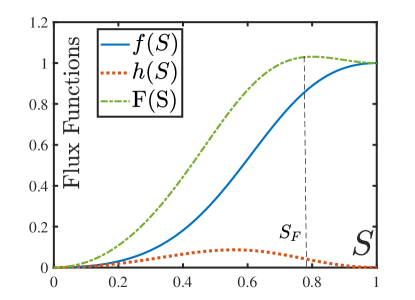
Figure 3: The functions $f(S),\;h(S)$ and $F(S)$ as given in Remark 2.2. Here $M=2$ and $N_{g}=4$.

2.4 Travelling wave formulation

Having derived the non-dimensional hysteretic two-phase flow System $(\tilde{\mathcal{P}})$, we investigate under which conditions travelling wave solutions exist. These are solutions of the form

$$S(z,t)=S(\xi),\;p(z,t)=p(\xi),\;\text{ with }\xi=ct-z,$$

where $S$ and $p$ are the wave profiles of saturation and pressure and $c\in\mathbb{R}$ the wave-speed. We seek travelling waves that satisfy

$$\begin{cases}\lim\limits_{\xi\to-\infty}S(\xi)=S_{B},\;\lim\limits_{\xi\to\infty}S(\xi)=S_{T},\\ \lim\limits_{\xi\to-\infty}p^{\prime}(\xi)=\lim\limits_{\xi\to\infty}p^{\prime}(\xi)=0,\end{cases}$$ (30)

where $S_{B}$ corresponds to an ‘initial’ saturation and $S_{T}$ to the injected saturation. The choice of $p^{\prime}(\pm\infty)=0$ ensures that the diffusive flux vanishes at $\xi=\pm\infty$. Substituting (30) into (28a) and (28b), and integrating (28a) one obtains

$$cS-\left(F(S,p)-h(S,p)p^{\prime}\right)=A,$$ (31a)

$$cS^{\prime}=\frac{1}{\tau}\mathcal{F}\left(S,p\right),$$ (31b)

where $\xi\in\mathbb{R}$ and $A$ is a constant of integration.

As was shown in [68] for the Richards equation, (30) and (31) do not automatically guarantee the existence of $\lim_{\xi\to\pm\infty}p(\xi)$. But if $p(\pm\infty)$ is well-defined then (31b) and the existence of $S(\pm\infty)$ forces $\lim_{\xi\to\pm\infty}{\mathcal{F}}(S(\xi),p(\xi))=0$. Recalling that ${\mathcal{F}}(S,p)=0$ iff $(S,p)\in{\cal H}$ we then have

$$\lim\limits_{\xi\to-\infty}p(\xi)=p_{B}\in[{p^{(i)}_{c}}(S_{B}),{p^{(d)}_{c}}(S_{B})],\;\lim\limits_{\xi\to\infty}p(\xi)=p_{T}\in[{p^{(i)}_{c}}(S_{T}),{p^{(d)}_{c}}(S_{T})].$$

We show later that $p_{B}$, interpreted as the initial pressure, can sometimes be chosen independently, whereas, $p_{T}$, when existing, is always fixed by the choice of $S_{B},S_{T}$ and $p_{B}$. Following the steps in [67, 68, 43] we obtain the Rankine-Hugoniot condition for wave-speed $c$, i.e.

$$c=\frac{F(S_{T},p_{T})-F(S_{B},p_{B})}{S_{T}-S_{B}}.$$ (32)

With this, system (31) can be rewritten as a dynamical system,

$$\mathrm{(TW)} S^{\prime}=\dfrac{1}{c\tau}\mathcal{F}\left(S,p\right)$$ , 5em. (33a)

$$\mathrm{(TW)} p^{\prime}=\mathcal{G}\left(S,p\right)$$ . (33b)

where

$$\mathcal{G}\left(S,p\right):=\frac{F(S,p)-\ell(S)}{h\left(S,p\right)}\text{ with }\ell(S):=F(S_{B},p_{B})+c(S-S_{B}).$$ (34)

Note that when $F$ is non-monotone (e.g. $N_{g}>M$ in Remark 2.2), the wave-speed $c$ can be positive or negative depending on the values of $S_{B}$ and $S_{T}$.

We study all possible solutions of system (TW) for $\tau>0$. They serve as viscous profiles of admissible shocks of the limiting Buckley-Leverett equation. Existence conditions for solutions of (TW) act as admissibility/entropy conditions for the corresponding shocks.

The solutions of (TW) are investigated under three different scenarios.

• No hysteresis in relative permeabilities, i.e. $\zeta^{(i)}=\zeta^{(d)}$ for $\zeta\in\{f,h\}$. Furthermore, $N_{g}$ is sufficiently small so that $F$ satisfies properties stated for $f^{(j)}$ in (P5). For $F$ as in Remark 2.2 this is satisfied if $N_{g}\leq M$.

• $N_{g}$ and $\tau$ sufficiently small; relative permeabilities are hysteretic.

A third scenario where $N_{g}$ is large so that $F$ is non-monotone is discussed briefly at the end of Section 3.

3 No relative permeability hysteresis and small $N_{g}$ (Scenario A)

In the absence of relative permeability hysteresis, the functions $f,\;h,\;F$ and ${\cal G}$ depend on $S$ only. We explicitly state the properties of $F$ as a result of (P5), (P6) and Remark 2.2.

1. $F\in C^{2}\left([0,1]\right),\;{F}^{\prime}(S)>0$ for $0<S<1,\;F(0)=0,\;F\left(1\right)=1$. Moreover, a unique $S_{o}\in(0,1)$ exists such that

   $$F^{\prime\prime}(S_{o})=0,\;F^{\prime\prime}(S)>0\text{ for }0<S<S_{o}\text{ and }F^{\prime\prime}(S)<0\text{ for }S_{o}<S<1.$$

Figure 4: (left) The saturations $S_{B},\;\underline{S},\;\bar{S},\;\tilde{S},\;\alpha$ and $\beta(\alpha)$ for Scenario A. (right) The functions $\beta$, $\gamma$ and $\bar{\gamma}$ (assuming (41)) and the definitions of $S_{*}$ and $S^{*}$ for $S_{B}<\underline{S}$.

3.1 Preliminaries

Throughout this paper we restrict ourselves to relatively small values of $S_{B}$. Specifically, we assume

$$0<S_{B}<S_{o}.$$ (35)

First let us take $S_{B}\leq\underline{S}$, where $\underline{S}$ is the saturation at which $F^{\prime}(\underline{S})=\frac{1-F(\underline{S})}{1-\underline{S}}$. The convex-concave behaviour of $F$ implies $\underline{S}<S_{o}$. For later purpose, and with reference to Figure 4 (left), we introduce the additional saturations $S_{B}<\tilde{S}<\bar{S}<1$, where $\tilde{S}$ is the saturation at which $F(S)$ intersects the line connecting $(S_{B},F(S_{B}))$ and $(1,1)$, and where $\bar{S}$ is the saturation for which $F^{\prime}(\bar{S})=\frac{F(\bar{S})-F(S_{B})}{\bar{S}-S_{B}}$. Then to each $\alpha\in[\tilde{S},\bar{S}]$ corresponds a unique $\beta\in[\bar{S},1]$ such that $(\beta,F(\beta))$ is the third intersection point between the graph of $F$ and the chord through $(S_{B},F(S_{B}))$ and $(\alpha,F(\alpha))$, see Figure 4 (left). This defines the function

$$\begin{cases}\beta:[\tilde{S},\bar{S}]\to[\bar{S},1],\;\beta(\bar{S})=\bar{S},\;\beta(\tilde{S})=1,\\ \beta(\alpha)\text{ is strictly decreasing}.\end{cases}$$ (36)

Later in this section a second function $\gamma=\gamma(\alpha)$ is introduced as one of the roots of the equation

$$\int_{S_{B}}^{\gamma(\alpha)}{\cal G}(S;S_{B},\alpha)dS=0\text{ for }S_{B}\leq\alpha\leq\bar{S}.$$ (37)

Here ${\cal G}(S;S_{B},\alpha)$ is the expanded notation of ${\cal G}$ from (34) for the $p$ independent case:

$${\cal G}(S;S_{B},\alpha)=\tfrac{F(S)-\ell(S;S_{B},\alpha)}{h(S)}\text{ with }\ell(S;S_{B},\alpha)=F(S_{B})+\tfrac{F(\alpha)-F(S_{B})}{\alpha-S_{B}}(S-S_{B}).$$

A typical sketch of ${\cal G}(S;S_{B},\alpha)$ for different values of $\alpha$ is shown in Figure 5. Note that

$${\cal G}(S;S_{B},\alpha)\text{ decreases with respect to }\alpha\in[S_{B},\bar{S}]\text{ and }$$ (38)

$${\cal G}(S;S_{B},\alpha)\begin{cases}\left.\begin{aligned} <0&\text{ for }S_{B}<S<\alpha\\ >0&\text{ for }S>\alpha\end{aligned}\right\}&\text{ when }S_{B}<\alpha<\tilde{S},\\ \left.\begin{aligned} <0&\text{ for }S_{B}<S<\alpha\\ >0&\text{ for }\alpha<S<\beta(\alpha)\\ <0&\text{ for }\beta(\alpha)<S<1\end{aligned}\right\}&\text{ when }\tilde{S}<\alpha<\bar{S}.\\ \end{cases}$$ (39)

Since,

$${\cal G}(S;S_{B},\alpha)=\begin{cases}\mathcal{O}(\tfrac{1}{k_{rn}(S)})&\text{ when }\alpha\not=\tilde{S},\\[1.99997pt] \mathcal{O}(\tfrac{1-S}{k_{rn}(S)})&\text{ when }\alpha=\tilde{S},\end{cases}$$ (40)

as $S\nearrow 1$, we have for most practical applications

$${\cal G}(S;S_{B},\alpha)\text{ is non-integrable near $S=1$ for each }S_{B}\leq\alpha\leq\bar{S}.$$ (41)

This is the case for Brooks-Corey permeabilities with $q\geq 2$, see Remark 2.2.

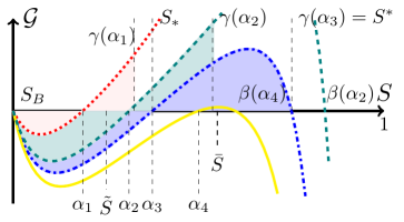
Figure 5: The plot of ${\cal G}(S;S_{B},\alpha)$ for different values of $\alpha$. Here $\alpha_{1}<\tilde{S}<\alpha_{2}<\alpha_{3}=S_{*}<\alpha_{4}<\bar{S}<S^{*}$. Values of $\gamma$ and $\beta$ are also shown. Note that, $\beta(\alpha_{1})$ and $\gamma(\alpha_{4})$ do not exist.

Returning to equation (37), we note that $\gamma=S_{B}$ is the trivial solution. Properties (39) and (40) imply the existence of a second (non-trivial) solution $\gamma=\gamma(\alpha)$ for $\alpha\geq S_{B}$. It satisfies $\gamma(S_{B})=S_{B}$, $\gamma(\alpha)$ increases, $\gamma(\alpha)>\alpha$ for $\alpha>S_{B}$. Moreover, if (41) is satisfied then $\gamma(\tilde{S})<1$. This shows the existence of $\gamma(\alpha)$ in a right neighbourhood of $S=\tilde{S}$. The solution in this case exists up to $\alpha=S_{*}\in(\tilde{S},\bar{S})$ where $\gamma(\alpha)$ and $\beta(\alpha)$ intersect: $\gamma(S_{*})=\beta(S_{*})=:S^{*}$. Further, if (41) holds, then a third solution $\gamma=\bar{\gamma}$ exists for $\tilde{S}<\alpha<S_{*}$. It decreases in $\alpha$ with $\bar{\gamma}(\tilde{S})=1$ and $\bar{\gamma}(S_{*})=S^{*}$. When (41) is not satisfied, the existence of $S_{*}$ and a third solution depends on the specific form of $k_{rn}(S)$. The solutions of (37) and the function $\beta(\alpha)$ are sketched in Figure 4 (right).

For $S_{B}\in(\underline{S},S_{o})$, $\beta(\alpha)$ and $\gamma(\alpha)$ can similarly be defined, although the domain where $\beta(\alpha)$ is defined is different. In this case the intersection of $\beta(\alpha)$ and the second solution $\gamma(\alpha)$ is guaranteed irrespective of (41) since $\int^{\bar{S}}_{S_{B}}{\cal G}(S;S_{B},\bar{S})dS<0$ and $\int^{1}_{S_{B}}{\cal G}(S;S_{B},1)dS>0$. This is because ${\cal G}(S;S_{B},\bar{S})<0$ for $S_{B}<S<\bar{S}$ and ${\cal G}(S;S_{B},1)>0$ for $S_{B}<S<1$. Since we use the second solution $\gamma=\gamma(\alpha)$ only, we summarize its properties in the following proposition.

Proposition 3.1.

Assume either (41) or $S_{B}\in(\underline{S},S_{o})$. Let $\gamma$ be the increasing (unique) solution of (37). Then it is defined in the interval $[S_{B},S_{*}]$ where $S_{*}\in(\tilde{S},\bar{S})$ is such that $\gamma(S_{*})=\beta(S_{*})=:S^{*}$. Further, $\gamma(S_{B})=S_{B}$, $\gamma(\alpha)>\alpha$ for $\alpha>S_{B}$ and $\gamma(\alpha)<\beta(\alpha)$ for $\alpha<S_{*}$ in the common domain of definition of $\beta$ and $\gamma$.

Remark 3.1.

For simplicity, we assume (41) for the rest of the discussion. This guarantees the existence of a $(S_{*},S^{*})$ pair. The methods presented in this paper can also be applied to analyse the case when $\beta(\alpha)$ and $\gamma(\alpha)$ are not intersecting. The results are briefly discussed in Section 3.2.

Next we turn to system (TW) where, for the time being, we take

$$S_{B}<S_{T}\leq\bar{S}.$$ (42)

Since (TW) is autonomous, it is convenient to represent solutions as orbits in the $(S,p)$-plane, or rather, in the strip $\{(S,p):0\leq S\leq 1,\;p\in\mathbb{R}\}$. Moreover, orbits are same for any shift in the independent variable $\xi$. Therefore we may set without loss of generality, see [68, 43],

$$S(0)=\frac{1}{2}(S_{B}+S_{T}).$$ (43)

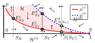
Figure 6: The $S$-$p$ phase plane and the direction of orbits for Scenario A with $\tilde{S}\leq S_{T}\leq\bar{S}$. The regions ${\cal H},\;{\mathcal{H}^{(i)}},\;{\mathcal{H}^{(d)}}$ and the equilibrium lines are marked.

Equilibrium points of (TW) are

$$E_{K}^{j}\equiv(K,p^{(j)}_{c}(K)),\text{ where }K\in\{S_{B},S_{T}\}\text{ and }j\in\{i,d\}.$$

If $\tilde{S}\leq S_{T}<\bar{S}$, a third pair exists for $K=\beta(S_{T})$. The points $E^{j}_{K}$ and the direction of the orbits are indicated in Figure 6. By the special nature of the function $\mathcal{F}$, we have in fact that all points of the segments $\overline{E^{i}_{K}E^{d}_{K}}$ are equilibrium points. Boundary conditions (30) are satisfied if an orbit connects the segments $\overline{E^{i}_{S_{B}}E^{d}_{S_{B}}}$ and $\overline{E^{i}_{S_{T}}E^{d}_{S_{T}}}$. As shown in [43], an orbit can leave $\overline{E^{i}_{S_{B}}E^{i}_{S_{B}}}$ only from the lowest point $E^{i}_{S_{B}}$. Then it enters region ${\mathcal{H}^{(i)}}$ where it moves monotonically with respect to $S$ as a consequence of the sign in the right hand side of equation (33a): if $p<{p^{(i)}_{c}}(S)$ we have $S^{\prime}>0$.

Due to this monotonicity one can alternatively describe an orbit leaving $E^{i}_{S_{B}}$ as a function of the saturation as long as it belongs to ${\mathcal{H}^{(i)}}$. For given $\tau>0$ and $S_{T}$ satisfying (42), let $w(S)=w(S;\tau,S_{T})$ denote this function. Then

$$w(S_{B};\tau,S_{T})={p^{(i)}_{c}}(S_{B})$$ (44a)

$$\text{ and }w(S;\tau,S_{T})<{p^{(i)}_{c}}(S)\text{ in a right neighbourhood of }S_{B}.$$ (44b)

As in [68, 43], we deduce from (TW) that $w$ should satisfy

$$w^{\prime}(S;\tau,S_{T})=\frac{c\tau{\cal G}(S;S_{B},S_{T})}{{p^{(i)}_{c}}(S)-w(S;\tau,S_{T})}\text{ for }S>S_{B}.$$ (45)

Using techniques from [68, 43], one can show that initial value problem (45), (44a) has a unique local solution $w(S;\tau,S_{T})$ that satisfies (44b).

Remark 3.2.

Conversely one recovers the orbit $(S(\xi),p(\xi))$ by substituting $w$ into (33a). Using (43) this gives

$$\xi=c\tau\int^{S(\xi)}_{\tfrac{1}{2}(S_{B}+S_{T})}\frac{d\varrho}{{p^{(i)}_{c}}(\varrho)-w(\varrho;\tau,S_{T})}d\varrho\text{ and }p(\xi)=w(S(\xi);\tau,S_{T}).$$

Rewriting (45) as

$$({p^{(i)}_{c}}-w)(w-{p^{(i)}_{c}})^{\prime}+({p^{(i)}_{c}}-w){p^{(i)}_{c}}^{\prime}=c\tau{\cal G}(S;S_{B},S_{T}),$$

we find recalling (P1) that

$$(({p^{(i)}_{c}}-w)^{2})^{\prime}=2({p^{(i)}_{c}}-w){p^{(i)}_{c}}^{\prime}-2c\tau{\cal G}(S;S_{B},S_{T})\leq-2c\tau{\cal G}(S;S_{B},S_{T})\text{ in }\{w<{p^{(i)}_{c}}\}.$$ (46)

Integrating this inequality from $S_{B}$ to $S$ gives the lower bound

$$\left.\begin{aligned} &w(S;\tau,S_{T})>{p^{(i)}_{c}}(S)-\sqrt{2c\tau\Phi(S)}\text{ in }\{w<{p^{(i)}_{c}}\},\\ &\text{ where }\Phi(S)=\Phi(S;S_{B},S_{T}):=-\int_{S_{B}}^{S}{\cal G}(\varrho;S_{B},S_{T})d\varrho.\end{aligned}\right\}$$ (47)

With $S_{T}$ satisfying (42), properties (39)-(41) and Proposition 3.1 imply

$$\left.\begin{aligned} &\Phi(S)>0\text{ for }S_{B}<S<\gamma(S_{T})\\ &\Phi(S_{B})=\Phi(\gamma(S_{T}))=0\end{aligned}\right\} \text{ when }S_{B}<S_{T}\leq S_{*},$$ (48a)

$$\text{ and }\left.\begin{aligned} &\Phi(S)>0\text{ for }S_{B}<S<1\\ &\lim\limits_{S\nearrow 1}\Phi(S)=+\infty\end{aligned}\right\} \text{ when }S_{*}<S_{T}\leq\bar{S}.$$ (48b)

Observe that, depending on $S_{B}$, $S_{T}$ and $\tau$, the interval where $w(S)<{p^{(i)}_{c}}(S)$ is either $(S_{B},1]$ if $w(S)$ and ${p^{(i)}_{c}}(S)$ do not intersect, or $(S_{B},S_{i})$ with $S_{i}\leq 1$ in case there is an intersection at $S=S_{i}$. In the latter case, it follows immediately from (46) that we must have,

Proposition 3.2.

Suppose there exists $S_{i}\in(S_{B},1)$ such that $w(S)<{p^{(i)}_{c}}(S)$ for $S_{B}<S<S_{i}$ and $w(S_{i})={p^{(i)}_{c}}(S_{i})$. Then ${\cal G}(S_{i};S_{B},S_{T})\geq 0$.

Hence, if the orbit exits through the capillary pressure curve ${p^{(i)}_{c}}$, it can only do so at points where ${\cal G}\geq 0$. From the discussion above, one defines

$$S_{m}(\tau,S_{T})=\sup\{S\in(S_{B},1):w(\varrho;\tau,S_{T})<{p^{(i)}_{c}}(\varrho)\text{ for all }S_{B}<\varrho<S\},$$ (49)

which is the upper limit of the interval on which $w$ exists. Then we have

Proposition 3.3.

• If $S_{B}<S_{T}\leq S_{*}$, then $S_{T}\leq S_{m}(\tau,S_{T})<\gamma(S_{T})$ for all $\tau>0$;

• If $S_{*}<S_{T}\leq\bar{S}$ and $w(\beta(S_{T});\tau,S_{T})<{p^{(i)}_{c}}(\beta(S_{T}))$, then $S_{m}(\tau,S_{T})=1$ and $\lim\limits_{S\nearrow 1}w(S)=-\infty$.

Proof.

(a) The lower bound follows from Proposition 3.2. To show the upper bound, observe that if $S_{m}(\tau,S_{T})\geq\gamma(S_{T})$, then $w(\gamma(S_{T}))\leq{p^{(i)}_{c}}(\gamma(S_{T}))$. This directly contradicts the strict inequality in (47) since $\Phi(\gamma(S_{T}))=0$.

(b) Since ${\cal G}(\cdot;S_{B},S_{T})<0$ in $(\beta(S_{T}),1)$, Proposition 3.2 and (47), (48a) imply $S_{m}(\tau,S_{T})=1$. Since (47) holds for all $S<1$ and since $w^{\prime}<0$ in a left neighbourhood of $S=1$, let us suppose that $\lim_{S\nearrow 1}w(S;\tau,S_{T})=-L$ ($L>0$). Then equation (45) and property (41) give $w^{\prime}\not\in L^{1}$ near $S=1$, contradicting the boundedness of $w$.∎∎

In Figure 7 we sketch the behaviour of $w(S;\tau,S_{T})$ in ${\mathcal{H}^{(i)}}$. The existence of orbits as in Figure 7 (left) is a direct consequence of the behaviour of the lower bound (47). Orbits as in Figure 7 (right) need more attention since the case $S_{m}(\tau,S_{T})<\beta(S_{T})$, represented by $\tau_{3}$, remains to be discussed. We make the behaviour as sketched in Figure 7 (right) precise in a number of steps.

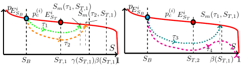
Figure 7: Sketch of orbits represented by $w(S;\tau,S_{T})$. (left) $S_{T,1}\in(S_{B},S_{*}]$, $\tau_{1}<\tau_{2}$; (right) $S_{T,2}\in(S_{*},\bar{S}]$, $\tau_{3}<\tau_{4}$.

We start with the following

Remark 3.3.

In the context of this section the wave-speed (32) reduces to

$$c=\frac{F(S_{T})-F(S_{B})}{S_{T}-S_{B}}.$$

From assumption (A1) it follows that there is a one-to-one correspondence between $c$ and $S_{T}\in[S_{B},\bar{S}]$. Writing $c=c(S_{T})$, we have $c(S_{B})=F^{\prime}(S_{B})$, $c(\bar{S})=F^{\prime}(\bar{S})$ and $\frac{dc}{dS_{T}}>0$ in $[S_{B},\bar{S}]$.

Next, we give a general monotonicity result.

Proposition 3.4 (Monotonicity).

Let $S_{B}$ satisfy (35).

• For a fixed $S_{T}\in(S_{B},\bar{S}]$ and any pair $0<\tau_{1}<\tau_{2}$,

  $$w(\cdot;\tau_{2},S_{T})<w(\cdot;\tau_{1},S_{T})\text{ in }\{w(\cdot;\tau_{1},S_{T})<{p^{(i)}_{c}}(\cdot)\}$$

  and

  $$S_{m}(\tau_{1},S_{T})<S_{m}(\tau_{2},S_{T})\text{ if }S_{T}<S_{m}(\tau_{2},S_{T})\leq\beta(S_{T});$$

• For fixed $\tau>0$ and any pair $S_{B}<S_{T,1}<S_{T,2}\leq\bar{S}$,

  $$w(\cdot;\tau,S_{T,2})<w(\cdot;\tau,S_{T,1})\text{ in }\{w(\cdot;\tau,S_{T,1})<{p^{(i)}_{c}}(\cdot)\}$$

  and

  $$S_{m}(\tau,S_{T,1})<S_{m}(\tau,S_{T,2})\text{ if }S_{T,2}\leq S_{m}(\tau,S_{T,2})\leq\beta(S_{T,2}).$$

Proof.

We argue as in [69, 67]. The key idea is to introduce the function

$$u=\frac{({p^{(i)}_{c}}-w)}{\sqrt{d}}\text{ with }d=c(S_{T})\tau.$$ (50)

Using (45) one obtains for $u$ the equation

$${u}^{\prime}(S;\tau,S_{T})=\frac{1}{\sqrt{d}}{p^{(i)}_{c}}^{\prime}(S)-\frac{{\cal G}(S;S_{B},S_{T})}{u(S;\tau,S_{T})}.$$ (51)

Clearly, $u|_{S_{B}}=0$ and $u>0$ in a right neighbourhood of $S_{B}$. Since ${\cal G}|_{S_{B}}=0$ as well, one finds from (51) and the sign of $u$

$$u^{\prime}(S_{B};\tau,S_{T})=-\frac{{p^{(i)}_{c}}^{\prime}(S_{B})}{2}\left[\sqrt{\dfrac{1}{d}-4\tfrac{{\cal G}^{\prime}(S_{B};S_{B},S_{T})}{({p^{(i)}_{c}}^{\prime}(S_{B}))^{2}}}-\dfrac{1}{\sqrt{d}}\right]>0$$

since ${\cal G}^{\prime}(S_{B};S_{B},S_{T})<0$. Using (38), Remark 3.3 and some elementary algebra

$$u^{\prime}(S_{B};\tau_{1},S_{T})<u^{\prime}(S_{B};\tau_{2},S_{T}) \text{ in case }(a),$$ (52a)

$$u^{\prime}(S_{B};\tau,S_{T,1})<u^{\prime}(S_{B};\tau,S_{T,2}) \text{ in case }(b).$$ (52b)

(a) From (52a), $u_{1}(\cdot):=u(\cdot;\tau_{1},S_{T})<u(\cdot;\tau_{2},S_{T})=:u_{2}(\cdot)$ in a right n eighbourhood of $S_{B}$. We claim that $u_{1}$ and $u_{2}$ do not intersect in $\{u_{1}>0\}$. Suppose, to the contrary, there exists $S_{i}>S_{B}$ such that $u_{1}(S)<u_{2}(S)$ for $S_{B}<S<S_{i}$ and $u_{1}(S_{i})=u_{2}(S_{i})$. Thus ${u_{1}}^{\prime}(S_{i})\geq{u_{2}}^{\prime}(S_{i})$. Evaluating (51) at $S_{i}$ gives

$${u_{1}}^{\prime}(S_{i})=\frac{{p^{(i)}_{c}}^{\prime}(S_{i})}{\sqrt{d_{1}}}-\frac{{\cal G}(S_{i};S_{B},S_{T,1})}{u_{1}(S_{i})}<\frac{{p^{(i)}_{c}}^{\prime}(S_{i})}{\sqrt{d_{2}}}-\frac{{\cal G}(S_{i};S_{B},S_{T,2})}{u_{2}(S_{i})}={u_{2}}^{\prime}(S_{i}),$$

a contradiction.

If $S_{T}<S_{m}(\tau_{2},S_{T})\leq\beta(S_{T})$, the $u$-monotonicity gives $S_{m}(\tau_{1},S_{T})\leq S_{m}(\tau_{2},S_{T})$. We rule out the equality by contradiction. Suppose $S_{m}(\tau_{1},S_{T})=S_{m}(\tau_{2},S_{T})=:S_{m}$. Then

$$u_{1}<u_{2}\text{ in }(S_{B},S_{m}).$$

Integrating equation (51) from $S_{T}$ to $S_{m}$ gives

$$u_{2}(S_{T})-u_{1}(S_{T})=({p^{(i)}_{c}}(S_{T})-{p^{(i)}_{c}}(S_{m}))\left(\tfrac{1}{\sqrt{d_{2}}}-\tfrac{1}{\sqrt{d_{1}}}\right)+\int^{S_{m}}_{S_{T}}{\cal G}\left(\tfrac{1}{u_{2}}-\tfrac{1}{u_{1}}\right).$$ (53)

Since ${\cal G}>0$ in $(S_{T},S_{m})$ for $S_{T}<S_{m}\leq\beta(S_{T})$, the term in the right of (53) is negative, yielding a contradiction.

(b) Using (38) this part is demonstrated along the same lines. Details are omitted. ∎∎

Remark 3.4.

To complement Proposition 3.4, we further state that

$$S_{m}(\tau_{1},S_{T})=S_{T}\text{ if }S_{m}(\tau_{2},S_{T})=S_{T}\text{ and }S_{m}(\tau_{2},S_{T})=1\text{ if }S_{m}(\tau_{1},S_{T})=1.$$

The statements follow directly from the ordering of the orbits.

So far we have shown the monotonicity of the orbits. However, the question of continuous variation is still open. This is addressed in the following results.

Proposition 3.5 (Continuous dependence of $w$).

Let $v={p^{(i)}_{c}}-w$. In the context of Proposition 3.4 and with $\Phi$ defined in (47) we have

• $0<v^{2}(S;\tau_{2},S_{T})-v^{2}(S;\tau_{1},S_{T})<2c(\tau_{2}-\tau_{1})\Phi(S)$ for $S_{B}<S\leq S_{m}(\tau_{1},S_{T})$;

• $0<v^{2}(S;\tau,S_{T,2})-v^{2}(S;\tau,S_{T,1})<2(c(S_{T,2})\,\Phi(S;S_{B},S_{T,2})-c(S_{T,1})\,\Phi(S;S_{B},S_{T,1}))$ for $S_{B}<S\leq S_{m}(\tau,S_{T,1})$;

Proof.

As shown earlier in this section, $v$ satisfies the equation

$$(v^{2})^{\prime}=2v{p^{(i)}_{c}}^{\prime}-2c\tau{\cal G}\text{ in }\{v>0\}.$$

Integrating this equation and using Proposition 3.4 and $\Phi$ from (47) gives the desired inequalities. ∎∎

Corollary 3.1 (Continuous dependence of $S_{m}$).

Let $\tau_{0}>0$ and $S_{T_{0}}$ be fixed such that $S_{m}(\tau_{0},S_{T_{0}})\leq\beta(S_{T_{0}})$. Then for any small $\varepsilon>0$, there exists $\delta=\delta(\varepsilon;\tau_{0},S_{T_{0}})$ so that $|S_{m}(\tau,S_{T})-S_{m}(\tau_{0},S_{T_{0}})|<\varepsilon$ if $\max\{|\tau-\tau_{0}|,|S_{T}-S_{T_{0}}|\}<\delta$ and $S_{m}(\tau,S_{T})<\beta(S_{T})$.

Proof.

We only demonstrate continuity with respect to $\tau$. Proving the continuity with respect to $S_{T}$ follows the same lines. We therefore take $S_{T}=S_{T_{0}}$ and drop its dependence from the notation for simplicity. Consider first $\tau>\tau_{0}$ and $S_{T_{0}}<\beta(S_{T_{0}})$. Recalling $v(S_{m}(\tau_{0});\tau_{0})=0$, Proposition 3.5 gives

$$0<v(S_{m}(\tau_{0});\tau)<\sqrt{2c(\tau-\tau_{0})\Phi(S_{m}(\tau_{0}))},$$

where $\Phi(S_{m}(\tau_{0}))>0$ by (48) and Proposition 3.3. For any given (small) $\varepsilon>0$ and with reference to Figure 8 choosing $\delta<\frac{{p^{(i)}_{c}}(S_{m}(\tau_{0}))-{p^{(i)}_{c}}(S_{m}(\tau_{0})+\varepsilon)}{2c\Phi(S_{m}(\tau_{0}))}$ we have

$$w(S_{m}(\tau_{0}),\tau)>{p^{(i)}_{c}}(S_{m}(\tau)+\varepsilon)\text{ for all }\tau-\tau_{0}<\delta.$$

Since $w^{\prime}>0$, this implies the continuity of $\tau>\tau_{0}$.

Next let $\tau<\tau_{0}$ and $S_{T_{0}}\leq\beta(S_{T_{0}})$. Now we have from Proposition 3.5

$$0<v(S_{m}(\tau);\tau_{0})<\sqrt{2c(\tau_{0}-\tau)\Phi(S_{m}(\tau))}.$$ (54)

Since $v(\cdot,\tau_{0})\in C([S_{B},S_{m}(\tau_{0})])$, $v(S_{m}(\tau_{0}),\tau_{0})=0$ and $v(\cdot,\tau_{0})>0$ in $(S_{B},S_{m}(\tau_{0}))$, the continuity of $S_{m}$ follows directly from (54). ∎∎

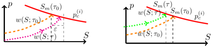
Figure 8: Behaviour of $w$ close to $S_{m}$: (left) $\tau>\tau_{0}$ and (right) $\tau<\tau_{0}$.

Now we are in a position to describe how $S_{m}$ behaves for different combinations of $S_{T}$ and $\tau$.

Proposition 3.6.

Let $S_{B}$ satisfy (35) and fix $S_{T}\in(S_{B},\bar{S}]$. Then there exists a $\tau_{m}(S_{T})>0$ such that

$$S_{m}(\tau,S_{T})=S_{T}\text{ for all }0<\tau\leq\tau_{m}(S_{T})\text{ and }S_{m}(\tau,S_{T})>S_{T}\text{ for all }\tau>\tau_{m}(S_{T}).$$

Proof.

The proof is based on Proposition 2.1 of [43] and Lemma 4.5 of [69]. Let us define the function $\ell_{r}(S)={p^{(i)}_{c}}(S)+r(S-S_{T})$ for $r>0$ and the constant $\underline{P}=\min_{S\in(S_{B},\bar{S})}\{-{p^{(i)}_{c}}^{\prime}(S)\}>0$. We show that for $\tau$ small enough there exists an $r>0$ for which the curves $w(S)$ and $\ell_{r}(S)$ do not intersect. Specifically

$$\ell_{r}(S)<w(S;\tau,S_{T})<{p^{(i)}_{c}}(S)\text{ for all }r>r^{-}\in(0,\underline{P})\text{ and }S\in(S_{B},S_{T}).$$ (55)

This directly shows that $w(S_{T})={p^{(i)}_{c}}(S_{T})=\ell_{r}(S_{T})$ meaning $S_{m}(\tau,S_{T})=S_{T}$.

Assuming the contrary, let $S_{i}\in(S_{B},S_{T})$ be the coordinate at which $w(S;\tau,S_{T})$ and $\ell_{r}(S)$ intersect for the first time. Since $w(S_{B})={p^{(i)}_{c}}(S_{B})>\ell_{r}(S_{B})$, one gets

$$({p^{(i)}_{c}}-w)(S_{i})=r(S_{T}-S_{i})\text{ and }\tfrac{c\tau{\cal G}(S_{i})}{r(S_{T}-S_{i})}=w^{\prime}(S_{i})\leq{\ell_{r}}^{\prime}(S_{i})={p^{(i)}_{c}}^{\prime}(S_{i})+r.$$ (56)

Recalling that ${\cal G}(S_{T})=0$ and taking $m_{0}(S_{T})=\sup_{S\in[S_{B},S_{T}]}{\cal G}^{\prime}(S;S_{B},S_{T})<\infty$ we get

$$\frac{{\cal G}(S_{i})}{S_{i}-S_{T}}\leq m_{0}(S_{T}).$$

Combining this with (56) results in the inequality $r^{2}-r\underline{P}+c\tau m_{0}\geq 0$. The roots of the quadratic expression on the left hand side of this inequality motivates us to define

$$\bar{\tau}_{m}=\frac{\underline{P}^{2}}{4cm_{0}(S_{T})}\text{ and }r^{\pm}=\frac{\underline{P}}{2}\left[1\pm\sqrt{1-\tfrac{\tau}{\bar{\tau}_{m}}}\right].$$ (57)

It directly follows that the inequality in (56) is not satisfied if $0<\tau<\bar{\tau}_{m}$ and $r\in(r^{-},r^{+})\subset(0,\underline{P})$. In this case one has $w(S)>\ell_{r}(S)$ for $S\in(S_{B},S_{T})$ and consequently, (55) holds. Note that $\tau>\bar{\tau}_{m}$ does not necessarily imply that $S_{m}(S_{T},\tau)>S_{T}$. For this purpose, we define

$$\tau_{m}(S_{T}):=\sup\{\tau:S_{m}(S_{T},\tau)=S_{T}\}\geq\bar{\tau}_{m}>0.$$ (58)

Using [68, Proposition 4.2(b)], which states that

$$w(S;\tau,S_{T})\to-\infty\text{ as }\tau\to\infty\text{ for all }S\in(S_{B},S_{T}],$$ (59)

we get from Corollary 3.1, $\tau_{m}(S_{T})<\infty$.∎∎

We consider now the case $\tau>\tau_{m}(S_{T})$. Proposition 3.3 guarantees that $S_{m}(S_{T},\tau)<\gamma(S_{T})\leq\beta(S_{T})$ if $S_{B}<S_{T}\leq S_{*}$. However, for $S_{T}>S_{*}$ it is unclear whether $S_{m}(S_{T},\tau)$ is bounded by $\beta(S_{T})$ or not. We show below that a $\tau_{c}=\tau_{c}(S_{T})$ exists in this case such that $S_{m}(S_{T},\tau)\in(S_{T},\beta(S_{T})]$ if $\tau\in(\tau_{m}(S_{T}),\tau_{c}(S_{T})]$ implying from Proposition 3.3 that $S_{m}(S_{T},\tau)=1$ for all $\tau>\tau_{c}(S_{T})$.

Proposition 3.7.

Let $S_{B}$ satisfy (35). Then the following holds:

• For each $S_{T}\in(S_{*},\bar{S})$, there exists a unique $\tau_{c}=\tau_{c}(S_{T})$ such that

  $$S_{m}(\tau_{c},S_{T})=\beta(S_{T}).$$

• The function $\tau_{c}(\cdot)$ is strictly decreasing and continuous on $[S_{*},\bar{S}]$. One has $\tau_{c}(S_{T})\to\infty$ as $S_{T}\searrow S_{*}$ and $\tau_{c}(\bar{S})=\bar{\tau}=\tau_{m}(\bar{S})>0$.

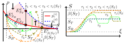
Figure 9: (left) Ordering of the orbits in the $S$-$p$ phase plane for $S_{*}<S_{T}<\bar{S}$ and $\tau\leq\tau_{c}(S_{T})$. (right) The behaviour of the orbits in the $\xi$-$S$ plane for $\tau\leq\tau_{c}(S_{T})$.

Proof.

(a) Suppose no $\tau_{c}(S_{T})$ exists such that $S_{m}(\tau_{c},S_{T})=\beta(S_{T})$, meaning $S_{m}(\tau,S_{T})<\beta(S_{T})$ for all $\tau>0$. Combined with (59), this implies that for large enough $\tau$, a $S_{1}\in[S_{T},\beta(S_{T})]$ exists for which $w(S_{1})=0$. From (45) it is evident that $w(S_{T})\leq w(S)$, in particular $w(S_{T})<w(S_{1})=0$. Moreover, (47) gives the lower bound $w(S)\geq w(S_{T})\geq{p^{(i)}_{c}}(S_{T})-\sqrt{2c\tau\Phi(S_{T})}\geq-\sqrt{2c\tau\Phi(S_{T})}$ for all $S\in[S_{B},S_{m}(\tau,S_{T})]$. Multiplying both sides of (51) by $u$, integrating from $S_{B}$ to $S_{1}$ and using the above inequality we get

$$-\dfrac{1}{2}{p^{(i)}_{c}}^{2}(S_{B}) =\int_{S_{B}}^{S_{1}}(c\tau{\cal G}(S;S_{B},S_{T})+{p^{(i)}_{c}}^{\prime}(S)w(S;c,\tau))dS$$

$$\leq-c\tau\Phi(S_{1})+({p^{(i)}_{c}}(S_{B})-{p^{(i)}_{c}}(S_{1}))\sqrt{2c\tau\Phi(S_{T})}.$$

Since $\Phi(S_{1})>0$ (as stated in (48b)), this leads to a contradiction for $\tau\to\infty$. Hence, $S_{m}(\tau,S_{T})=\beta(S_{T})$ for some $\tau>0$. The uniqueness follows from Proposition 3.4.

(b) The monotonicity and continuity follows from Propositions 3.4 and 3.5 and Corollary 3.1. To show the limit for $S_{T}\searrow S_{*}$, assume that $\lim_{S_{T}\searrow S_{*}}\tau_{c}(S_{T})=\tau_{\infty}<\infty$. Let then $\tau>\tau_{\infty}$. Proposition 3.3 implies that $S_{m}(\tau,S_{*})<\beta(S_{*})$. Choose an $S_{T}>S_{*}$ such that $\beta(S_{T})\geq S_{m}(\tau,S_{*})$. Since $\tau>\tau_{c}(S_{T})$, we get that $w(S_{m}(\tau,S_{*});\tau,S_{T})\leq w(\beta(S_{T});\tau,S_{T})\leq{p^{(i)}_{c}}(\beta(S_{T}))$, implying $w(S_{m}(\tau,S_{*});\tau,S_{*})-w(S_{m}(\tau,S_{*});\tau,S_{T})\geq{p^{(i)}_{c}}(S_{m}(\tau,S_{*}))-{p^{(i)}_{c}}(\beta(S_{T}))$. This gives a contradiction when $S_{T}\searrow S_{*}$ since the right hand side goes to ${p^{(i)}_{c}}(S_{m}(\tau,S_{*}))-{p^{(i)}_{c}}(\beta(S_{*}))>0$, whereas the left hand side converges to 0 from Corollary 3.1.

The existence of a $\bar{\tau}>0$ is a consequence of the continuity of $\tau_{c}$ with $\bar{\tau}=\tau_{m}(\bar{S})\geq\bar{\tau}_{m}(\bar{S})$ following from Proposition 3.6. ∎∎

After the preliminary statements we are in a position to consider the solvability of (TW) for different ranges of $S_{T}$.

3.2 Problem (TW) with $S_{B}<S_{T}\leq\bar{S}$

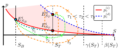
Figure 10: The different cases of $S_{B}<S_{T}<S_{*}$. The orbits are plotted for $0<\tau_{1}<\tau_{i}<\tau_{2}<\tau_{d}<\tau_{3}$.

We investigate the existence of an orbit connecting $(S_{B},{p^{(i)}_{c}}(S_{B}))$ and the segment $\overline{E^{i}_{S_{T}}E^{d}_{S_{T}}}$. Defining

$$\tau_{j}=\frac{({p^{(j)}_{c}}^{\prime}(S_{T}))^{2}}{4c{\cal G}^{\prime}(S_{T};S_{B},S_{T})}>0,\quad j\in\{i,d\},$$ (60)

the eigenvalues of the (TW) system associated with the equilibrium points $E^{j}_{S_{T}}$, $j\in\{i,d\}$ are

$$\lambda^{j}_{\pm}=\frac{{p^{(j)}}^{\prime}(S_{T})}{2c\tau}\left[1\pm\sqrt{1-\frac{\tau}{\tau_{j}}}\right]\text{ implying }\begin{cases}E^{j}_{S_{T}}\text{ is stable sink for }\tau\leq\tau_{j},\\ E^{j}_{S_{T}}\text{ is stable spiral sink for }\tau>\tau_{j}.\end{cases}$$

This immediately gives $\tau_{i}\geq\tau_{m}$ as no monotone orbit can connect with $E^{i}_{S_{T}}$ for $\tau>\tau_{i}$. The general behaviour of the orbits for $S_{T}\in(S_{B},S_{*}]$ are stated in

Theorem 3.1.

Under the assumptions of Scenario A, consider $S_{B}$ satisfying (35), $S_{T}\in(S_{B},S_{*}]$ and $\tau_{i}<\tau_{d}$. Let $(S,p)$ be the orbit originating from $(S_{B},{p^{(i)}_{c}}(S_{B}))$ satisfying (TW). Then, with reference to Figure 10, as $\xi\to\infty$ one gets

• If $0<\tau\leq\tau_{i}$, then either $S\to S_{T}$ and $p\to{p^{(i)}_{c}}(S_{T})$ monotonically with respect to $\xi$ through ${\mathcal{H}^{(i)}}$ (when $\tau\leq\tau_{m}$) or the orbit $(S,p)$ goes around $\overline{E^{i}_{S_{T}}E^{d}_{S_{T}}}$ finitely many times and ends up in either $E^{i}_{S_{T}}$ or $E^{d}_{S_{T}}$ (when $\tau_{m}<\tau\leq\tau_{i}$).

• If $\tau_{i}<\tau\leq\tau_{d}$, $(S,p)\to E^{d}_{S_{T}}$ after finitely many turns around $\overline{E^{i}_{S_{T}}E^{d}_{S_{T}}}$.

• If $\tau_{d}<\tau$, then $(S,p)$ revolves infinitely many times around $\overline{E^{i}_{S_{T}}E^{d}_{S_{T}}}$ while approaching it and (30) is satisfied.

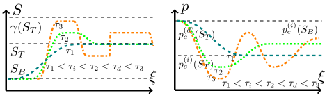
Figure 11: Typical behaviour of $S(\xi)$ (left) and $p(\xi)$ (right) for different values of $\tau$. Here profiles for three different $\tau$ values are plotted satisfying $0<\tau_{1}<\tau_{i}<\tau_{2}<\tau_{d}<\tau_{3}$. The $\xi=0$ coordinate is fixed by (43).

These statements are demonstrated by arguments from [43, Theorem 2.1 and Lemma 2.1 & 2.2]. We omit the details here. In Theorem 3.1 we have taken $\tau_{i}<\tau_{d}$ without loss of generality. In the $\tau_{i}>\tau_{d}$ case, the roles of the equilibrium points $E^{i}_{S_{T}}$ and $E^{d}_{S_{T}}$ are reversed. The typical behaviour of the $S$ and the $p$ profiles with respect to $\xi$ is given in Figure 11. Both $S$ and $p$ are monotone for $\tau<\tau_{i}$, whereas for $\tau_{i}<\tau<\tau_{d}$ they have finite number of local extrema and $p(+\infty)={p^{(d)}_{c}}(S_{T})$. For $\tau>\tau_{d}$, $S$ has infinitely many decaying local extrema, whereas $p$ has no limit. In particular, each $S$ maximum corresponds to a saturation overshoot. On the other hand, the oscillations in $p$ become wider, in line with the assumption $\lim_{\xi\to\infty}p^{\prime}(\xi)=0$. In this case, the segment $\overline{E^{i}_{S_{T}}E^{d}_{S_{T}}}$ becomes an $\omega$-limit set of the orbit.

Turning to the case, $S_{T}\in(S_{*},\bar{S})$, we define the two functions which will be used extensively below

Definition 3.1.

The functions $\hat{S}_{B},\;\check{S}_{B}:[0,\infty)\to(0,1]$ are such that

$$\check{S}_{B}(\tau)=\begin{cases}(\tau_{c})^{-1}(\tau)&\text{ for }\tau>\bar{\tau},\\ \bar{S}&\text{ for }0\leq\tau\leq\bar{\tau},\end{cases}\text{ and }\hat{S}_{B}(\tau)=\beta(\check{S}_{B}(\tau)).$$

Observe that, ${\check{S}_{B}}(\tau)$ is a strictly decreasing function whereas ${\hat{S}_{B}}(\tau)$ is a strictly increasing function for $\tau>\bar{\tau}$ and $\hat{S}_{B}(\tau)=\check{S}_{B}(\tau)=\bar{S}$ for $\tau\leq\bar{\tau}$. This is sketched in Figure 12. Numerically computed $\check{S}_{B}(\tau)$ and $\hat{S}_{B}(\tau)$ functions are shown in Figure 20.

Remark 3.5.

The case when $\beta(\alpha)$ does not intersect $\gamma(\alpha)$ is treated in a similar way. However, since orbits may intersect the line segment $\{S=1,p\leq 0\}$ in this case, a multivalued extension of ${p^{(i)}_{c}}$ at $S=1$ needs to be introduced, see [43, 68] for further details. With this, one shows that the function $\tau_{c}(S_{T})$ is well-defined in $[\tilde{S},\bar{S}]$. Then a $\tau_{\!{}_{B}}>0$ exists such that ${\check{S}_{B}}(\tau_{\!{}_{B}})=\tilde{S}$ and ${\hat{S}_{B}}(\tau_{\!{}_{B}})=1$. The subsequent results remain valid if $\hat{S}_{B}$ and $\check{S}_{B}$ are extended by

$$\check{S}_{B}(\tau_{\!{}_{B}})=\tilde{S}\text{ for }\tau>\tau_{\!{}_{B}},\text{ and }\hat{S}_{B}(\tau)=1\text{ for }\tau>\tau_{\!{}_{B}}.$$

With this in mind, we define the following sets:

$$\mathcal{A}=\{(S_{T},\tau):S_{B}<S_{T}<\bar{S},\;\tau<\tau_{c}(S_{T})\},$$

$$\mathcal{B}=\{(S_{T},\tau):\tau>\bar{\tau},\;\check{S}_{B}(\tau)<S_{T}<\hat{S}_{B}(\tau)\},$$

$$\mathcal{C}=\{(S_{T},\tau):\bar{S}<S<S^{*},\;\tau<\tau_{c}(\beta^{-1}(S_{T}))\}.$$ (61)

Figure 12: The sets $\mathcal{A}$, $\mathcal{B}$ and $\mathcal{C}$ and the functions $\check{S}_{B}(\tau)$, $\hat{S}_{B}(\tau)$.

Observe that, if $S_{T}<\bar{S}$ then only regions $\mathcal{A}$ and $\mathcal{B}$ are relevant. With $S_{o}$ defined in (A1), for $(S_{T},\tau)\in\mathcal{A}$ one has

Proposition 3.8.

For a fixed $S_{B}\in(0,S_{o})$ and $(S_{T},\tau)\in\mathcal{A}$, the orbit $(S,p)$ entering ${\mathcal{H}^{(i)}}$ from $E^{i}_{S_{B}}$ behaves according to statements (a),(b) and (c) of Theorem 3.1.

We discuss the remaining situations, $(S_{T},\tau)\in\mathcal{B}$ and $(S_{T},\tau)\in\mathcal{C}$ in the next section.

3.3 $(S_{T},\tau)\not\in\mathcal{A}$

Since $S_{T}>\check{S}_{B}(\tau)$, a TW cannot connect $S_{B}$ and $S_{T}$. However, a different class of waves is possible when $(S_{T},\tau)\in\mathcal{B}$.

Proposition 3.9.

For a fixed $S_{B}\in(0,S_{o})$ and $(S_{T},\tau)\in\mathcal{B}$, consider the system

$$\begin{cases}S^{\prime}=\dfrac{1}{c_{d}\tau}{\mathcal{F}}(S,p),\\[1.99997pt] p^{\prime}={\cal G}(S;\hat{S}_{B}(\tau),S_{T}),\end{cases}\text{ with }c_{d}=\frac{F(\hat{S}_{B}(\tau))-F(S_{T})}{\hat{S}_{B}(\tau)-S_{T}}.$$ (62)

For this system an orbit $(S_{d},p_{d})$ exists that connects $E^{d}_{\hat{S}_{B}(\tau)}$ for $\xi\to-\infty$ to $\overline{E^{i}_{S_{T}}E^{d}_{S_{T}}}$ for $\xi\to\infty$.

Proof.

Upon inspection of the eigen-directions for the system (62) around the equilibrium point $E^{d}_{\hat{S}_{B}(\tau)}$ one concludes that there is indeed an orbit $(S_{d},p_{d})$ that connects to $E^{d}_{\hat{S}_{B}(\tau)}$ as $\xi\to-\infty$ from the set ${\mathcal{H}^{(d)}}$ defined in (17). Moreover, from the direction of the orbits in this case, as shown in Figure 13 (left), it is apparent that after leaving $E^{d}_{\hat{S}_{B}(\tau)}$, $S_{d}$ decreases monotonically till the orbit either hits the curve $p={p^{(d)}_{c}}(S)$ for some $S\leq S_{T}$ or exits $\{S>S_{B}\}$ through the line $S=S_{B}$. We prove that it is not possible for the orbit to escape through $S=S_{B}$.

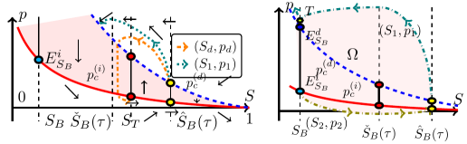
Figure 13: (left) The direction of orbits for the system (33a), (62) and the orbits $(S_{d},p_{d})$ and $(S_{1},p_{1})$. Here the orbit $(S_{d},p_{d})$ connects $E^{d}_{\hat{S}_{B}(\tau)}$ and $E^{i}_{S_{T}}$. (right) The domain $\Omega$ used in the divergence argument for the hypothetical case where $(S_{1},p_{1})$ crosses the line $S=S_{B}$.

To show this, consider the orbit $(S_{1},p_{1})$ that satisfies the original (TW) equations and enters ${\mathcal{H}^{(d)}}$ from $E^{d}_{\hat{S}_{B}(\tau)}$. We show that this orbit cannot cross the line $S=S_{B}$. The divergence argument presented in [18, 68, 43] is used for this purpose. To elaborate, assume that $(S_{1},p_{1})$ intersects the line $S=S_{B}$ at $T$. Consider the region $\Omega$, enclosed by the segments $\overline{E^{i}_{S_{B}}T}$, $\overline{E^{i}_{\hat{S}_{B}(\tau)}E^{d}_{\hat{S}_{B}(\tau)}}$, the orbit $(S_{1},p_{1})$ and the orbit $(S_{2},p_{2})$ that satisfies (TW) and connects $E^{i}_{S_{B}}$ to $E^{i}_{\hat{S}_{B}(\tau)}$, see Figure 13 (right). Introducing the vector-valued function $\overrightarrow{R}(S,p)=(\frac{1}{c\tau}{\mathcal{F}}(S,p),{\cal G}(S;S_{B},S_{T}))$ and deduces from (18),

$$\mathrm{div}\overrightarrow{R}=\frac{1}{c\tau}\frac{\partial{\mathcal{F}}}{\partial S}(S,p)=\frac{1}{c\tau}\begin{cases}{p^{(i)}_{c}}^{\prime}(S)&\text{ in }{\mathcal{H}^{(i)}},\\[-1.99997pt] 0&\text{ in }{\cal H},\\[-1.99997pt] {p^{(d)}_{c}}^{\prime}(S)&\text{ in }{\mathcal{H}^{(d)}}.\end{cases}$$

This gives a contradiction when the divergence theorem is applied to $\overrightarrow{R}$ in the domain $\Omega$: the integral of $\overrightarrow{R}$ over $\partial\Omega$ is non-negative whereas $\int_{\Omega}\mathrm{div}\overrightarrow{R}<0$ from (P1) and Figure 13 (right). Hence, the orbit $(S_{1},p_{1})$ intersects ${p^{(d)}_{c}}(S)$ at some $S\in(S_{B},\check{S}_{B}(\tau)]$.

The wave-speed corresponding to the orbit $(S_{d},p_{d})$ satisfies

$$c_{d}<\tfrac{F(\hat{S}_{B}(\tau))-F(S_{B})}{\hat{S}_{B}(\tau)-S_{B}}=c_{i},$$ (63)

$c_{i}$ being the speed of both $(S_{1},p_{1})$ and $(S_{2},p_{2})$ waves. Hence, by the continuity of the orbits with respect to $c$, as shown in Proposition 3.4, it is evident that $(S_{d},p_{d})$ intersects ${p^{(d)}_{c}}(S)$ for some $S_{d}>S_{B}$. From here, the rest of the proof is identical to the proof of Theorem 3.1, and follows the arguments in [43, Theorem 2.1 and Lemma 2.1 & 2.2]. ∎

From the results of Theorem 3.1 we further state

Corollary 3.2.

The orbit $(S_{d},p_{d})$ can monotonically go to $E^{d}_{S_{T}}$ only when $\tau\leq\frac{({p^{(d)}_{c}}^{\prime}(S_{T}))^{2}}{4c_{d}{\cal G}^{\prime}(S_{T};\hat{S}_{B}(\tau),S_{T})}$. For $\tau$ large enough, the orbit $(S_{d},p_{d})$ goes around $\overline{E^{i}_{S_{T}}E^{d}_{S_{T}}}$ infinitely many times while approaching it, and $\lim\limits_{\xi\to\pm\infty}p_{d}^{\prime}(\xi)=0$.

Observe that, if $(S_{T},\tau)\in\mathcal{C}$ then travelling waves do not exist between $S_{T}$ and $\hat{S}_{B}(\tau)$ since both are in the concave part of $F$ with $S_{T}>\hat{S}_{B}(\tau)$. Thus we have exhausted all the possibilities of connecting $S_{B}$ and $S_{T}$ with Theorem 3.1 and Proposition 3.9.

3.4 Entropy solutions to hyperbolic conservation laws

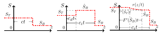
Figure 14: The entropy solutions for (left) $(S_{T},\tau)\in\mathcal{A}$, (center) $(S_{T},\tau)\in\mathcal{B}$ and (right) $(S_{T},\tau)\in\mathcal{C}$. Note that the solutions in the center and the right figures include non-classical shocks.

Under the conditions of Scenario A, we consider the Riemann problem

$$\dfrac{\partial S}{\partial t}+\dfrac{\partial F(S)}{\partial z}=0\text{ in }\mathbb{R}\times[0,\infty)$$ (64a)

$$\text{ with }S(z,0)=\begin{cases}S_{T}&\text{ for }z<0,\\ S_{B}&\text{ for }z>0.\end{cases}$$ (64b)

In the context of the viscous model discussed in this paper, we consider the Buckley-Leverett equation (64a) as the limit of System (27) for $N_{c}\searrow 0$. As a consequence, we only take into account those shock solutions of (64a) that have a viscous profile in the form of a travelling wave satisfying (TW). Such shocks are called admissible because they arise as the $N_{c}\to 0$ limit of TWs. In this sense, the entropy condition for shocks satisfying (64a) are equivalent to existence conditions for travelling waves satisfying (TW). This may lead to non-classical shocks violating the well-known Oleinik entropy conditions, see e.g. [69].

Here, we assume

$$0<S_{B}<S_{T}<1,$$ (65)

which is more general compared to (35) where the additional constraint of $S_{B}<S_{o}$ was imposed. This generalization is possible since $S_{B}>S_{o}$ simply implies that the sets $\mathcal{A},\;\mathcal{B}$ are empty. Our analysis can also be applied to derive the entropy conditions for the case $S_{B}>S_{T}$, however, for simplicity we restrict our discussion to (65).

$(S_{T},\tau)\in\mathcal{A}$

As in the usual Buckley-Leverett case (i.e. without dynamic capillarity and hysteresis in the regularised models) the solution is given by

$$S(z,t)=\begin{cases}S_{T}&\text{ for }z<ct,\\ S_{B}&\text{ for }z>ct,\end{cases}\text{ where }c=\frac{F(S_{T})-F(S_{B})}{S_{T}-S_{B}}.$$ (66)

Here, the shock satisfies the classical Oleinik condition.

$\underline{(S_{T},\tau)\in\mathcal{B}}$

In this case the admissible solution is composed of two shocks: an infiltration shock from $S_{B}$ to $\hat{S}_{B}(\tau)$, followed by a drainage shock from $\hat{S}_{B}(\tau)$ to $S_{T}$.

$$S(z,t)=\begin{cases}S_{T}&\text{ for }z<c_{d}t,\\ \hat{S}_{B}(\tau)&\text{ for }c_{d}t<z<c_{i}t,\\ S_{B}&\text{ for }z>c_{i}t,\end{cases}\text{ with }\begin{cases}c_{i}=\frac{F(\hat{S}_{B}(\tau))-F(S_{B})}{\hat{S}_{B}(\tau)-S_{B}},\\[1.99997pt] c_{d}=\frac{F(\hat{S}_{B}(\tau))-F(S_{T})}{\hat{S}_{B}(\tau)-S_{T}}.\end{cases}$$ (67)

Note that this solution violates the Oleinik condition [47]. Both shocks are under compressive [37].

$\underline{(S_{T},\tau)\in\mathcal{C}}$

The solution in this case violates again the Oleinik entropy condition. It consists of an infiltration shock from $S_{B}$ to $\hat{S}_{B}(\tau)$ followed by a rarefaction wave from $\hat{S}_{B}(\tau)$ to $S_{T}$,

$$S(z,t)=\begin{cases}S_{T}&\text{ for }z<F^{\prime}(S_{T})t,\\ r(z/t)&\text{ for }F^{\prime}(S_{T})t<z<F^{\prime}(\hat{S}_{B}(\tau))t,\\ \hat{S}_{B}(\tau)&\text{ for }F^{\prime}(\hat{S}_{B}(\tau))t<z<c_{i}t,\\ S_{B}&\text{ for }z>c_{i}t,\end{cases}$$ (68)

with $r(\cdot)$ satisfying

$$F^{\prime}(r(\zeta))=\zeta,\text{ for }F^{\prime}(S_{T})\leq\zeta\leq F^{\prime}(\hat{S}_{B}(\tau)).$$ (69)

Since $F$ is concave for $S\in[\hat{S}_{B}(\tau),S_{T}]$, $F^{\prime}$ is monotone implying that $r(\cdot)$ is well-defined. We observe that in the last two cases the solution features a plateau-like region. This plateau appears and grows in time since the speeds of the drainage shock and of the end point of the rarefaction wave are lesser than the speed of the infiltration shock. Interestingly, the saturation of the plateau only depends on ${p^{(i)}_{c}}$ and not on ${p^{(d)}_{c}}$. To be more specific, although the viscous profile consisting of a travelling wave connecting $E^{d}_{\hat{S}_{B}}$ and $\overline{E^{i}_{S_{T}}E^{d}_{S_{T}}}$ depends on ${p^{(d)}_{c}}$, the shock solution resulting from it, in the hyperbolic limit, does not. However, the role of the drainage curve in the entropy solutions become evident in Scenario B, which is discussed in the next section.

In the absence of hysteresis and for linear higher order terms, which correspond to constant $k$ and linear $p_{c}$-$S$ dependence, in [69, Section 6] it is proved that the non-standard entropy conditions discussed here are entropy dissipative for the entropy $U(s)=\frac{1}{2}s^{2}$. However, such an analysis is beyond the scope of this paper. The solution profiles for the Riemann problem are shown in Figure 14.

Extension to the non-monotone $F$ case

The analysis so far can be extended to the case where $N_{g}$ is large resulting in $F$ being non-monotone. If $S_{F}\in(0,1)$ is the saturation where $F(S)$ attains its maximum (see Remark 2.2 and Figure 3), then the results obtained so far cover the case when $S_{T}$ and $S^{*}$ are below $S_{F}$. However, if $S_{T}>S_{F}$ then the TW study has to be conducted also from a $S_{T}$ perspective, not only from the $S_{B}$ one. In this scenario, since fronts having negative speeds and thus moving towards $S_{T}$ become possible, one has to consider the functions $\hat{S}_{T}(\tau)$, $\check{S}_{T}(\tau)$ for a fixed $S_{T}$, similar to $\hat{S}_{B}(\tau)$, $\check{S}_{B}(\tau)$ from Definition 3.1 for fixed $S_{B}$. Due to the symmetry in the behaviour of the fronts approaching $S_{B}$, respectively $S_{T}$, some of the results obtained so far extend straightforwardly to the non-monotone case. However, a detailed analysis is much more involved and therefore left for future research because of the following two reasons:

1. Depending on the relative positions of $S_{B}$, $\hat{S}_{B}$, $S_{T}$ and $\hat{S}_{T}$, there are many sub-cases to consider. In this case up to three shocks are possible, traveling both forward and backward. Which of these shocks are admissible and how they are connected requires further analysis.

2. For a non-monotone $F$, when considering the hyperbolic limit in the absence of hysteresis or dynamic effects, the entropy solutions may include rarefaction waves with endpoints moving in opposite directions, forward and backward. When capillary hysteresis is included, preliminary numerical results have provided solutions incorporating two rarefaction waves, one with endpoints travelling backward and another one with endpoints travelling forward, and a stationary shock at $z=0$. Such solutions still need to be analysed further.

4 Hysteretic relative permeabilities and small $N_{g}$ (Scenario B)

For Scenario B, the flux function $F(S,p)$ is composed of $F^{(j)}=f^{(j)}+N_{g}h^{(j)}$ for $j\in\{i,d\}$ and $\bar{F}=\bar{f}+N_{g}\bar{h}$ such that

$$F(S,p)=\begin{cases}F^{(d)}(S)&\text{ if }(S,p)\in{\mathcal{H}^{(d)}},\\ \bar{F}(S,p)&\text{ if }(S,p)\in{\cal H},\\ F^{(i)}(S)&\text{ if }(S,p)\in{\mathcal{H}^{(i)}}.\end{cases}$$ (70)

It has the following properties

1. $F\in C({\bf{\cal W}})$, $\bar{F}\in C^{2}({\cal H})$, $\partial_{p}F>0$ in ${\cal H}$ and $F^{(i)}$, $F^{(d)}$ satisfy properties stated for $F$ in (A1). Additionally, $F^{(d)}(S)>F^{(i)}(S)$ for $0<S<1$.

In this scenario, $S_{B}$ can be taken in the entire interval $(0,1)$ and $p_{B}$ can be chosen independently as long as $(S_{B},p_{B})\in{\cal H}$, i.e.

$$0<S_{B}<1\text{ and }p_{B}\in[{p^{(i)}_{c}}(S_{B}),{p^{(d)}_{c}}(S_{B})].$$ (71)

This is different from Scenario A where $S_{B}$ is restricted to the interval $(0,S_{o})$ and $p_{B}$ is fixed to $p_{B}={p^{(i)}_{c}}(S_{B})$.

We first introduce some notation.

Definition 4.1.

For $k\in\{B,T\}$ let $E_{k}=(S_{k},p_{k})$ and $U_{k}=(S_{k},F(S_{k},p_{k}))$ (see Figure 15 (left)). We define the saturations $\bar{S}_{j}$, $j\in\{i,d\}$ as the $S$-coordinates of the tangent points to $F^{(j)}(S)$ from $U_{B}$ such that $\bar{S}_{i}\geq S_{B}$ and $\bar{S}_{d}\leq S_{B}$.

Observe that, the saturations $\bar{S}_{j}$, for $j\in\{i,d\}$, are functions of $U_{B}$. The properties of $F^{(j)}$ further ensure that they are well defined. If $S_{B}$ is such that ${F^{(i)}}^{\prime\prime}(S_{B})\leq 0$ and $p_{B}={p^{(i)}_{c}}(S_{B})$ then $\bar{S}_{i}=S_{B}$. Similarly if ${F^{(d)}}^{\prime\prime}(S_{B})\geq 0$ and $p_{B}={p^{(d)}_{c}}(S_{B})$ then $\bar{S}_{d}=S_{B}$.

The existence of travelling waves is analysed for the following two cases:

$$\text{ Case (i): }S_{B}<S_{T}\leq\bar{S}_{i},\text{ and }\text{ Case (ii) : }\bar{S}_{d}\leq S_{T}<S_{B}.$$

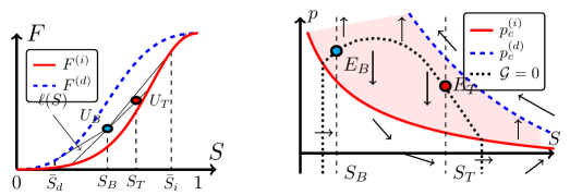
Figure 15: (left) The graphs of $F^{(i)}$ and $F^{(d)}$, together with the saturations $\bar{S}_{i},\;\bar{S}_{d}$ and the points $U_{B},\;U_{T}$. (right) The orbit directions for Case (i) for two equilibrium points $E_{B}$ and $E_{T}$. The black dotted curve represents points where ${\cal G}(S,p)=0$, implying $p^{\prime}=0$.

Regarding the choice of $p_{T}$, we have the following

Proposition 4.1.

Let $S_{B}$ and $S_{T}$ be as in Case (i) or Case (ii). Then any solution of (TW) that connects $E_{B}$ and $E_{T}$ can only exist if $p_{T}={p^{(i)}_{c}}(S_{T})$ or $p_{T}={p^{(d)}_{c}}(S_{T})$.

Proof.

Since $E_{T}$ is an equilibrium point, ${\mathcal{F}}(S_{T},p_{T})=0$, which implies that $p_{T}\in[{p^{(i)}_{c}}(S_{T}),{p^{(d)}_{c}}(S_{T})]$. The directions of the orbits for $p_{T}$ in this interval are displayed in Figure 15 (right). We proceed by introducing the set

$${\cal H}_{0}=\{(S,p):S\in(0,1),\;p\in\mathbb{R}\text{ such that }{\cal G}(S,p)=0\}.$$

It corresponds to the black dotted curve in Figure 15 (right). Let $\ell=\ell(S)$, defined in (34), be the line passing through $U_{B}$ and $U_{T}$. If $\ell$ intersects $F^{(i)}$ at $S=S_{H}$, then the vertical half-line $\{(S_{H},p):p<{p^{(i)}_{c}}(S_{H})\}$ lies in ${\cal H}_{0}$ due to the definition of $F$ in (70). Concerning $F^{(d)}$, $\ell$ has either zero, one or two intersection points, see Figure 16 (left). In the latter case, as before, ${\cal H}_{0}$ contains one or two vertical half-lines as shown in the (right) plot of Figure 16. However, this aspect plays no major role in the analysis below.

Every point in the set ${\cal H}_{0}\cap{\cal H}$ is an equilibrium point. However, all points in the set ${\cal H}_{0}\cap\mathrm{int}({\cal H})$ (the interior of ${\cal H}$ being referred to as $\mathrm{int}({\cal H})$ here) are unstable and as follows from Figure 15 (right), no orbit can reach these points as $\xi\to\infty$. This eliminates all other possibilities to reach $E_{T}$ as $\xi\to\infty$ except for $p_{T}={p^{(i)}_{c}}(S_{T})$ and $p_{T}={p^{(d)}_{c}}(S_{T})$. ∎

We now consider the two cases separately.

4.1 Case (i): $S_{B}<S_{T}\leq\bar{S}_{i}$

The main result of this section is

Proposition 4.2.

Assume (71) and let $S_{T}\in(S_{B},\bar{S}_{i}]$, $p_{T}={p^{(i)}_{c}}(S_{T})$ and $F^{(i)}(S_{T})>F(S_{B},p_{B})$. Then a $\tau^{*}_{i}(S_{T})>0$ exists such that for all $\tau<\tau^{*}_{i}(S_{T})$ there is an orbit satisfying (TW) and connecting $E_{B}$ to $E_{T}$.

Proof.

Consider the orbit $(S_{(i)},p_{(i)})$ that leaves $E_{B}$ vertically through the half-line $\{S=S_{B},p<p_{B}\}$. The directions of the orbits in ${\cal H}$ imply that $(S_{(i)},p_{(i)})$ intersects ${p^{(i)}_{c}}(S)$ and enters ${\mathcal{H}^{(i)}}$ (the region under the graph of ${p^{(i)}_{c}}$) at some finite $\xi\in\mathbb{R}$, see Figure 16 (right). In ${\mathcal{H}^{(i)}}$ its motion is governed by the system

$$\begin{cases}{S_{(i)}}^{\prime}=\frac{1}{c_{(i)}\tau}({p^{(i)}_{c}}(S_{(i)})-p_{(i)}),\;\\ {p_{(i)}}^{\prime}={\cal G}_{i}(S_{(i)}):={\cal G}(S_{(i)},{p^{(i)}_{c}}(S_{(i)})),\end{cases}\text{ with }c_{(i)}=\tfrac{F^{(i)}(S_{T})-F(S_{B},p_{B})}{S_{T}-S_{B}}>0.$$ (72)

Note that, ${\cal G}_{i}(S)=(F^{(i)}(S)-\ell(S))/h^{(i)}(S)$. The system (72) has exactly the same structure as (TW) described in Section 3. Defining $\tau_{i}^{*}(S_{T})$ similar to $\tau_{m}$ in Proposition 3.6, the result follows directly. ∎

Remark 4.1.

Observe that, the construction fails if $F^{(i)}(S_{T})<F(S_{B},p_{B})$ which is intuitive since the overall process is not infiltration in this case. If one prescribes a flux $F=F_{T}$ at $\xi\to\infty$ which is less than $F(S_{B},p_{B})$, then Propositions 4.1 and 4.2 forces the saturation at $\xi\to\infty$ to be $S_{T}=(F^{(d)})^{-1}(F_{T})<S_{B}$, reducing the problem to Case (ii). However, if one fixes the saturation $S_{T}$ so that $F(S_{B},p_{B})>F^{(i)}(S_{T})$, then we get a frozen profile with a $p_{T}\in({p^{(i)}_{c}}(S_{T}),{p^{(d)}_{c}}(S_{T}))$ that satisfies $F(S_{T},p_{T})=F(S_{B},p_{B})$. This is explained further in Section 5.2. We set $\tau^{*}_{i}(S_{T})=\infty$ in this case.

Proposition 4.2 implies the following:

Corollary 4.1.

Under the assumptions of Proposition 4.2, let $S_{(i)}(\underline{\xi})=S$ for some $S\in(S_{B},S_{T}]$ and $\underline{\xi}\in\mathbb{R}$. Define $\underline{w}(S;\tau):=p_{(i)}(\underline{\xi})<{p^{(i)}_{c}}(S)$. Then $\lim\limits_{\tau\to 0}\underline{w}(S;\tau)={p^{(i)}_{c}}(S)$.

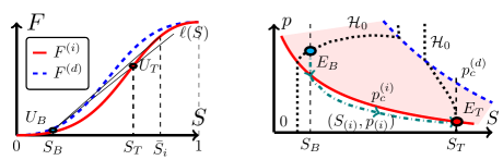
Figure 16: $U_{B}$, $U_{T}$, $\ell(S)$ used in Proposition 4.2 in the $S$-$F$ plane. (right) The $S$-$p$ plane and the orbit $(S_{(i)},p_{(i)})$ for Case (i) with $F^{(i)}(S_{T})>F(S_{B},p_{B})$ and $\tau<\tau^{*}_{i}(S_{T})$.

Here, $\underline{w}$ is the counterpart of $w$ defined in Section 3 for Scenario A. The proof of Corollary 4.1 is based on the inequality (47) which is satisfied in this case by $\underline{w}$. From Corollary 4.1 one obtains that for Case (i), if $\tau\searrow 0$, meaning that if the dynamic capillarity is vanishing, then the orbit follows either the scanning curve, here the line segment $\{S=S_{B},{p^{(i)}_{c}}(S_{B})<p<p_{B}\}$, or the infiltration curve ${p^{(i)}_{c}}$. The result is analogous to the results for capillary hysteresis given in [68, Section 3].

4.2 Case (ii): $\bar{S}_{d}\leq S_{T}<S_{B}$ and stability of plateaus

The counterpart of Proposition 4.2 for Case (ii) is (see also Figure 17),

Proposition 4.3.

Assume (71) and let $S_{T}\in[\bar{S}_{d},S_{B})$, $p_{T}={p^{(d)}_{c}}(S_{T})$ and $F^{(d)}(S_{T})<F(S_{B},p_{B})$. Then a $\tau^{*}_{d}(S_{T})>0$ exists such that for all $\tau<\tau^{*}_{d}(S_{T})$ there is an orbit $(S_{(d)},p_{(d)})$ satisfying (TW) and connecting $E_{B}$ to $E_{T}$. Moreover, for a fixed $S_{(d)}=S\in[S_{T},S_{B})$, one has $p_{(d)}\to{p^{(d)}_{c}}(S)$ as $\tau\to 0$.

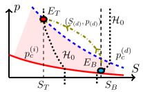
Figure 17: The orbit $(S_{(d)},p_{(d)})$ for Case (ii) with $F^{(d)}(S_{T})<F(S_{B},p_{B})$ and $\tau<\tau^{*}_{d}(S_{T})$.

Finally, we investigate a special case related to the development of stable saturation plateaus in infiltration experiments. For $S_{B}\in(0,1)$, and $S_{T}\in(S_{B},1)$ a stable plateau is formed when an infiltration wave, from $S_{B}$ to $S_{P}\in(S_{T},1)$, followed by a drainage wave, from $S_{P}$ to $S_{T}$, both have the same speed resulting in the width of the plateau to remain constant. This is different from the plateaus described in (67) where the speeds of the infiltration and the drainage fronts are necessarily different. The existence of stable saturation plateaus has been widely studied experimentally [19, 64, 24] and numerically [59, 31]. Although results regarding stability of the plateau are available [59, 31], the mechanism behind its development is still not well understood. Here, we give an example where our analysis predicts that such a plateau will develop. Specifically, it occurs when $\tau>\tau^{*}_{i}(S_{T})$ and a direct monotone orbit from $E_{B}$ to $(S_{T},{p^{(i)}_{c}}(S_{T}))$ is no longer possible. This is verified numerically in Section 5.2.

Proposition 4.4.

Assume (71) and let $S_{T}\in(S_{B},1)$ be such that the line $\ell$ through $U_{B}=(S_{B},F(S_{B},p_{B}))$ and $U_{T}=(S_{T},F^{(d)}(S_{T}))$ in the $F$-$S$ plane intersects $F^{(i)}$ at some $S=S_{P}\in(S_{T},\bar{S}_{i})$. Consider the system (TW) with the wave-speed

$$c_{P}=\tfrac{F^{(d)}(S_{T})-F(S_{B},p_{B})}{S_{T}-S_{B}}=\tfrac{F^{(i)}(S_{P})-F(S_{B},p_{B})}{S_{P}-S_{B}}=\tfrac{F^{(i)}(S_{P})-F^{(d)}(S_{T})}{S_{P}-S_{T}}.$$

For this system, let $(S^{P}_{(i)},p^{P}_{(i)})$ be the orbit that passes through ${\mathcal{H}^{(i)}}$ and connects to the equilibrium point $(S_{B},p_{B})$ as $\xi\to-\infty$, described in Proposition 4.2. Similarly, let $(S^{P}_{(d)},p^{P}_{(d)})$ be the orbit passing through ${\mathcal{H}^{(d)}}$ and connecting to $(S_{P},{p^{(i)}_{c}}(S_{P}))$ as $\xi\to-\infty$, described in Proposition 4.3. Assume that $0<\tau<\max\{\tau^{*}_{i}(S_{P}),\tau^{*}_{d}(S_{T}))\}$ where the $\tau^{*}_{i}(S_{P})$ and the $\tau^{*}_{d}(S_{T})$ values correspond to the orbits $(S^{P}_{(i)},p^{P}_{(i)})$ and $(S^{P}_{(d)},p^{P}_{(d)})$ respectively. Then, $(S^{P}_{(i)},p^{P}_{(i)})\to(S_{P},{p^{(i)}_{c}}(S_{P}))$ as $\xi\to\infty$ and $(S^{P}_{(d)},p^{P}_{(d)})\to(S_{T},{p^{(d)}_{c}}(S_{T}))$ as $\xi\to\infty$.

The proof follows directly from Propositions 4.2 and 4.3.

4.3 Entropy solutions

We can now discuss the entropy solutions of the Riemann problem (64) under the assumptions of Scenario B. To be more specific, we give a selection criteria for the solutions of the system

$$\begin{cases}\dfrac{\partial S}{\partial t}+\dfrac{\partial F(S,p)}{\partial z}=0,\\[5.0pt] p\in\frac{1}{2}({p^{(d)}_{c}}(S)+{p^{(i)}_{c}}(S))-\frac{1}{2}({p^{(d)}_{c}}(S)-{p^{(i)}_{c}}(S))\cdot{\rm sign}\left(\frac{\partial S}{\partial t}\right),\end{cases}\text{ in }\mathbb{R}\times[0,\infty)$$ (73)

$$\text{ with }S(z,0)=\begin{cases}S_{T}&\text{ for }z<0,\\ S_{B}&\text{ for }z>0,\end{cases}\text{ and }p(z,0)=p_{B}\text{ for }z>0.$$ (74)

We view (73) as the limit of ($\mathcal{P}$) when the capillary effects vanish. However, hysteresis is still present in the model.

Note that, $\tau$ still plays a role in determining the entropy solution despite being absent in (73). This is similar to what we saw in Section 3. However, the focus here being hysteresis in permeability and capillary pressure, for a fixed $S_{B}\in(0,1)$ we take

$$0<\tau<\min\left\{\inf\limits_{S_{T}\in(S_{B},\bar{S}_{i}]}\tau^{*}_{i}(S_{T}),\inf\limits_{S_{T}\in[\bar{S}_{d},S_{B})}\tau^{*}_{d}(S_{T})\right\}.$$ (75)

Observe that, (75) does not provide a void interval for $\tau$. To see this, note that $\tau^{*}_{i}(S_{T})$ is defined similar to $\tau_{m}$ in Proposition 3.6 and thus, it satisfies the inequality in (58), i.e. it has the positive quantity $\bar{\tau}_{m}$ as its lower bound. Although $\bar{\tau}_{m}$ in Proposition 3.6 actually depends on $S_{T}$, one sees from (57) that the values of $\bar{\tau}_{m}$ are bounded away from 0 uniformly with respect to $S_{T}$. Hence, $\tau^{*}_{i}(S_{T})$ is also bounded uniformly away from 0. Similar argument holds for $\tau^{*}_{d}(S_{T})$.

We now consider the cases $S_{T}>S_{B}$ and $S_{T}<S_{B}$ separately.

$S_{T}>S_{B}$

If $S_{T}\leq\bar{S}_{i}$ ($\bar{S}_{i}$ introduced in Definition 4.1) and $F^{(i)}(S_{T})>F(S_{B},p_{B})$ then the entropy solution is a shock:

$$S(z,t)=\begin{cases}S_{T}&\text{ for }z<c_{(i)}t,\\ S_{B}&\text{ for }z>c_{(i)}t,\end{cases}\text{ with }c_{(i)}=\frac{F^{(i)}(S_{T})-F(S_{B},p_{B})}{S_{T}-S_{B}}.$$ (76)

For $F^{(i)}(S_{T})<F(S_{B},p_{B})$, from Remark 4.1, the solution is (76) but with $c_{(i)}=0$, i.e. it is a stationary shock. However, if $S_{T}>\bar{S}_{i}$ then the solution becomes more complex, combining a rarefaction wave with a shock:

$$S(z,t)=\begin{cases}S_{T}&\text{ for }z<{F^{(i)}}^{\prime}(S_{T})t,\\ r_{(i)}(z/t)&\text{ for }{F^{(i)}}^{\prime}(S_{T})t<z<{F^{(i)}}^{\prime}(\bar{S}_{i})t,\\ \bar{S}_{i}&\text{ for }{F^{(i)}}^{\prime}(\bar{S}_{i})t<z<c_{(i)}t,\\ S_{B}&\text{ for }z>c_{(i)}t.\end{cases}$$ (77)

Here $r_{(i)}(\cdot)$ satisfies

$${F^{(i)}}^{\prime}(r_{(i)}(\zeta))=\zeta,\text{ for }{F^{(i)}}^{\prime}(S_{T})\leq\zeta\leq{F^{(i)}}^{\prime}(\bar{S}_{i}).$$

$S_{T}<S_{B}$

If $S_{T}\geq\bar{S}_{d}$ then the entropy solution for $F(S_{B},p_{B})>F^{(d)}(S_{T})$ is the shock

$$S(z,t)=\begin{cases}S_{T}&\text{ for }z<c_{(d)}t,\\ S_{B}&\text{ for }z>c_{(d)}t,\end{cases}\text{ with }c_{(d)}=\frac{F(S_{B},p_{B})-F^{(d)}(S_{T})}{S_{B}-S_{T}},$$ (78)

and for $F(S_{B},p_{B})<F^{(d)}(S_{T})$ it is (78) with $c_{(d)}=0$. If $S_{T}<\bar{S}_{d}$ then the solution has a similar structure to (77), i.e.

$$S(z,t)=\begin{cases}S_{T}&\text{ for }z<{F^{(d)}}^{\prime}(S_{T})t,\\ r_{(d)}(z/t)&\text{ for }{F^{(d)}}^{\prime}(S_{T})t<z<{F^{(d)}}^{\prime}(\bar{S}_{d})t,\\ \bar{S}_{d}&\text{ for }{F^{(d)}}^{\prime}(\bar{S}_{d})t<z<c_{(d)}t,\\ S_{B}&\text{ for }z>c_{(d)}t,\end{cases}$$ (79)

with the function $r_{(d)}(\cdot)$ satisfying

$${F^{(d)}}^{\prime}(r_{(d)}(\zeta))=\zeta,\text{ for }{F^{(d)}}^{\prime}(S_{T})\leq\zeta\leq{F^{(d)}}^{\prime}(\bar{S}_{d}).$$

5 Numerical results

For the numerical experiments, we solve $(\tilde{\mathcal{P}})$ (System (28)) in a domain $\left(z_{in},z_{out}\right)$, where $z_{in}<0$ and $z_{out}>0$. As an initial condition for the saturation variable, we choose a smooth and monotone approximation of the Riemann data:

$$S\left(z,0\right)=\begin{cases}S_{T}\text{ for }z<-l,\\[1.99997pt] \frac{\left(S_{B}+S_{T}\right)}{2}+\frac{\left(S_{T}-S_{B}\right)}{4l^{3}}z\cdot(z^{2}-3l^{2})\text{ for }-l\leq z\leq l,\\[1.99997pt] S_{B}\text{ for }z>l.\end{cases}$$ (80)

Here, $l$ is a smoothing parameter, $S_{T}$ denotes the saturation induced by a certain injection rate and $S_{B}$ is the initial saturation within the porous medium. In order to model the capillary pressure, a van Genuchten parametrisation is considered, i.e.

$$p_{c}^{(j)}(S)=\Lambda_{j}(S^{-\frac{1}{m_{j}}}-1)^{1-m_{j}},\;j\in\left\{i,d\right\}.$$

In the remainder of this section we use the following parameter set: $\Lambda_{i}=3.5$, $m_{i}=0.92$, $\Lambda_{d}=7$ and $m_{d}=0.9$. To solve $(\tilde{\mathcal{P}})$ numerically, for $n\in\mathbb{N}\cup\{0\}$ and $t_{0}=0$, we solve within the time step

$$\left[t_{n},t_{n+1}\right]\text{ of width }\Delta t_{n}=t_{n+1}-t_{n},$$

the elliptic problem

$$-\frac{\partial}{\partial z}\left(F\left(S,p\right)+h\left(S,p\right)\frac{\partial p}{\partial z}\right)=\frac{1}{\tau}\mathcal{F}\left(S,p\right),$$

with respect to the pressure variable $p$. For a given $S$, this is a nonlinear elliptic problem and to solve it, a linear iterative scheme is employed which is referred to as the L-scheme in literature [52, 39, 42]:

$$L\left(p_{n}^{i}-p_{n}^{i-1}\right)-\frac{\partial}{\partial z}\left(F\left(S_{n},p_{n}^{i-1}\right)+h\left(S_{n},p_{n}^{i-1}\right)\frac{\partial p_{n}^{i}}{\partial z}\right)=\frac{1}{\tau}\mathcal{F}\left(S_{n},p_{n}^{i-1}\right).$$

Here, $p_{n}^{i}$ denotes the pressure at the $i^{\mathrm{th}}$ iteration and $p_{n}^{0}=p\left(z,t_{n}\right)$. On closer examination, the L-scheme corresponds to a linearization of the nonlinear problem, since for each iteration a linear equation in the unknown pressure variable $p_{n}^{i}$ is solved. For Scenario A the parameter $L$ is set to $L=\frac{1}{\tau}$ to ensure convergence of the L-scheme [52, 43] and for Scenario B the modified variant of the L-scheme is used [42, 68] to speed up the convergence, since in this scenario the stiffness matrix has to be recomputed in every iteration. A standard cell centered finite volume scheme is considered for discretizing the linearised elliptic problem in space. Having the pressure variable $p_{n}$ and the saturation variable $S_{n}$ for $t=t_{n}$ at hand, we update the saturation as follows:

$$S_{n+1}=S_{n}+\frac{\Delta t_{n}}{\tau}\mathcal{F}\left(S_{n},p_{n}\right).$$

5.1 Numerical results for Scenario A

First we illustrate the theoretical findings of Scenario A. The boundary conditions with respect to the pressure variable are of Neumann type at $z=z_{in}$ and of Dirichlet type at $z=z_{out}$:

$$p^{\prime}\left(z_{in},t\right)=0\text{ and }p\left(z_{out},t\right)={p^{(i)}_{c}}(S_{B})\text{ for all }t>0.$$ (81)

The boundaries of the domain are given by: $z_{in}=-10$ and $z_{out}=500$. Since we do not include hysteresis in the relative permeabilites, the flux function $F$ depends only on $S$ and is determined by:

$$f\left(S\right)=\frac{S^{2}}{S^{2}+\left(1-S\right)^{2}}\text{ and }N_{g}=1.$$

The numerical results presented in this subsection are related to $t=t_{\text{end}}=300$. For the parameters of the initial condition, we take:

$$S_{B}=0.1,\quad S_{T}=0.4\;\text{ and }l=1.$$

Based on these data, some of the variables and constants occurring in Section 3.1 and Figure 4 are computed, i.e:

$$\tilde{S}\approx 0.3138,\;\bar{S}\approx 0.5909,\;S_{o}\approx 0.4393,\;S_{\ast}\approx 0.4111\text{ and }S^{\ast}\approx 0.8132.$$ (82)

Moreover, the curves for $\gamma$ and $\beta$ are determined (see Figure 18). Observe that, from our choice, $S_{B}<S_{o}$ and $S_{T}\in\left(S_{B},S_{*}\right]$.

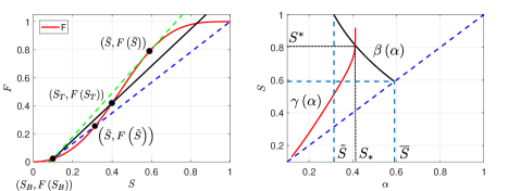
Figure 18: Fractional flow function $F$ for Scenario A (left). The characteristic points $\tilde{S}$, $\bar{S}$ and $S_{T}$ are shown. (right) Curves for $\gamma$ (red) and $\beta$ (black) corresponding to $F$. The intersection point of these curves is denoted by $\left(S_{\ast},S^{\ast}\right)$.

Next, the characteristic $\tau$-values for drainage and imbibition are computed. Using (60) and given parameters, we obtain:

$$\tau_{i}=0.0452\text{ and }\tau_{d}=0.2620.$$

Since the requirements listed in Theorem 3.1 are all fulfilled, we can compare the numerical results with the claims contained in the theorem. For this purpose, we choose $\tau$ from the following set:

$$\tau\in\left\{0.045,\;0.25,\;1.0,\;2.0\right\},$$

and study the resulting $S$-$p$ orbits. Considering Figure 19, it can be observed that for $\tau<\tau_{i}$ monotone saturation waves are produced by the numerical model linking $E_{S_{B}}^{i}$ and $E_{S_{T}}^{i}$. In the other cases, a saturation overshoot can be detected, where for $\tau_{i}<\tau<\tau_{d}$ the orbit ends up at the equilibrium point $E_{S_{T}}^{d}$ and for $\tau>\tau_{d}$ the orbits spiral around the segment $\overline{E_{S_{T}}^{i}E_{S_{T}}^{d}}$. If we choose larger values of $\tau$, the corresponding $S_{m}(\tau,S_{T})$ value of the orbit increases. This supports the claims of Corollary 3.1 and Proposition 3.4. Similar results including variation of saturation with $\xi$ can be found in [43].

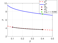
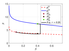
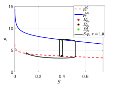
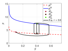
Figure 19: Orbits for different $\tau$ parameters in the $S$-$p$ plane.

The parameter choice considered so far, corresponds to the solution class $\mathcal{A}$ (see (61)), whose entropy solution consists of a single shock without any saturation overshoots (see Figure 21 (top)). However, there are two further solution classes, $\mathcal{B}$ and $\mathcal{C}$ (see (61)), arising in the context of Scenario A, represented by entropy solutions (67) and (68). In case of solution class $\mathcal{B}$, the entropy solution is given by saturation plateau that is formed by an infiltration wave followed by a drainage wave. The saturation at plateau level is denoted by $\hat{S}_{B}\left(\tau\right)$. For solution class $\mathcal{C}$, the entropy solution exhibits a rarefaction wave connecting $S_{T}$ with $\hat{S}_{B}\left(\tau\right)$, which is connected to $S_{B}$ by a shock.

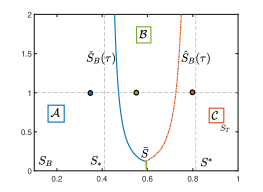
Figure 20: The $\hat{S}_{B}(\tau)$ and $\check{S}_{B}(\tau)$ curves computed for $S_{B}=0.1$. The characteristic saturations are as in (82). The corresponding Sets $\mathcal{A},\;\mathcal{B}$ and $\mathcal{C}$ along with $(S_{T},\tau)$ test pairs used in Figure 21 are shown.

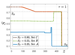
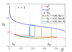
Figure 21: Numerical solutions corresponding to different $(S_{T},\tau)$ pairs from solution classes $\mathcal{A}$, $\mathcal{B}$ and $\mathcal{C}$, marked in Figure 20. Here, $\tau=1$ is fixed and $S_{T}$ is chosen from $\{0.35,0.55,0.8\}$. The (left) plot shows the variation of $S$ with $z$, whereas, the (right) plot shows $p$ vs. $S$. The saturation plateau for the Sets $\mathcal{B}$ and $\mathcal{C}$ is observed at $\hat{S}_{B}=.7158$.

To observe these cases numerically, we compute the $\hat{S}_{B}(\tau)$ and $\check{S}_{B}(\tau)$ curves introduced in Definition 3.1, see Figure 20. In the figure we fix $\tau=1$ and vary $S_{T}$ so that the pairs $(S_{T},\tau)$ belong to one of the sets $\mathcal{A},\;\mathcal{B}$ and $\mathcal{C}$. The results are shown in Figure 21 with the (left) plot showing the variation of $S$ with $z$, and the (right) plot showing the profiles in the $S$-$p$ phase plane. The curves corresponding to Set $\mathcal{A}$ show a direct travelling wave connecting $S_{B}$ and $S_{T}=0.35$. Some oscillatory behaviour around $S_{T}$ can be observed since $\tau$ is comparatively large, however, the existence of a single travelling wave between $S_{B}$ and $S_{T}$ implies that these states are connectable by an admissible shock in the hyperbolic limit. Next, choosing $S_{T}=0.55$, $(S_{T},\tau)$ lies in Set $\mathcal{B}$, and a solution consisting of an infiltration wave followed by a drainage wave is computed in accordance with the theory. Again, small oscillations are seen in the drainage wave part which is expected from Corollary 3.2 since $\tau$ is large. The resulting plateau has saturation $0.7158$, whereas, the prediction from Figure 20 is $\hat{S}_{B}(\tau)=0.7254$. Finally, for $S_{T}=0.8$, the pair $(S_{T},\tau)$ belongs to the Set $\mathcal{C}$. The numerical solution exhibits a shock-like structure followed by a plateau and they coincide with the infiltration wave of Set $\mathcal{B}$ on both plots of Figure 21. Moreover, a rarefaction wave between $\hat{S}_{B}\left(\tau\right)$ and $S_{T}$ is detected. Thus, we conclude that the saturation profiles in Figure 21 correspond to the entropy solutions depicted in Figure 14 and the numerical results are in agreement with the theory.

5.2 Numerical results for Scenario B

In case of Scenario B, we choose the following boundary conditions with respect to the pressure variable. As in the previous subsection, they are of Neumann type at $z=z_{in}$ and of Dirichlet type at $z=z_{out}$:

$$p^{\prime}\left(z_{in},t\right)=0\text{ and }p\left(z_{out},t\right)={p^{(d)}_{c}}(S_{B})\text{ for all }t>0.$$ (83)

Moreover, the boundaries of the domain are given by: $z_{in}=-10$ and $z_{out}=190$. To make matters interesting, contrary to the previous subsection, we do not start with an infiltration state for $S_{B}$, but with a drainage state. Due to the fact that we consider hysteresis both in the capillary pressure and relative permeabilities, fractional flow functions are introduced both for infiltration and for drainage. We use

$$f^{(i)}(S)=\frac{S^{2}}{S^{2}+3(1-S^{2})},\;f^{(d)}(S)=\frac{S^{2}}{S^{2}+2(1-S^{2})}\text{ with }N_{g}=0,$$

and define $F^{(i)}$ and $F^{(d)}$ accordingly. We verified numerically that if $S_{T}>S_{B}$ and $F^{(i)}(S_{T})<F(S_{B},p_{B})$ then the solution is frozen in time in the sense that $S(z,t)=S(z,0)$ for all $t>0$. This is what was discussed in Remark 4.1. To verify Propositions 4.2 and 4.3 and entropy solutions (76)-(79), we show two results: $S_{B}=S_{B,1}=0.3$, $S_{T}=S_{T,1}=0.95$ and $S_{B}=S_{B,2}=0.95$, $S_{T}=S_{T,2}=0.3$ both for $\tau=0.02$. Let the corresponding solutions be $(S_{(i)},p_{(i)})$ and $(S_{(d)},p_{(d)})$. Since $S_{T,1}>\bar{S}_{i}$ for the first case (see Definition 4.1) and $\tau$ is small, from (77) it is expected that the entropy solution will have a shock from $S_{B,1}$ to $\bar{S}_{i}$, followed by a rarefaction wave from $\bar{S}_{i}$ to $S_{T,1}$. This is exactly what is seen from the viscous profiles obtained numerically, see Figure 22. Similarly, for the second case, since $S_{T,2}<\bar{S}_{d}$ and $\tau$ is small, we see from Figure 22 a viscous solution resembling a drainage shock followed by a rarefaction wave, as predicted in (79).

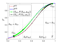
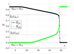
Figure 22: The viscous solutions for $S_{B,1}=0.3,\;S_{T,1}=0.95$ denoted by $(S_{(i)},p_{(i)})$ and $S_{B,2}=0.95,\;S_{T,2}=0.3$ denoted by $(S_{(d)},p_{(d)})$ with boundary conditions (83) and $\tau=0.02$ fixed. In the (left) plot, the solutions are shown in the $F$-$S$ plane and in the (right) plot the saturations are plotted as functions of $z$. The points $U_{B,1}$ and $U_{B,2}$ and the saturations $\bar{S}_{i}(U_{B,1})$ and $\bar{S}_{d}(U_{B,2})$, introduced in Definition 4.1, are marked. The results agree with the predictions of Propositions 4.2 and 4.3 and Section 4.3.

Next, we investigate whether a stable plateau is formed for suitable parameter values by an infiltration wave and an ensuing drainage wave, as predicted in Proposition 4.4. This happens only if $\tau>\tau^{*}_{i}(S_{T})$, since in this case, a monotone connection between $(S_{B},p_{B})$ and $(S_{T},{p^{(i)}_{c}}(S_{T}))$ does not exist. To this end, in the numerical experiment we have used the following parameters:

$$S_{B}=0.3,\quad S_{T}=0.5\;\text{ and }\tau=0.5.$$

For a stable saturation plateau, the velocities of the infiltration wave, connecting $S_{B}$ and $S_{P}$, and the drainage wave, connecting $S_{P}$ and $S_{T}$, have to be equal, i.e. if $c^{P}_{(i)}$ and $c^{P}_{(d)}$ are denoting the two wave-speeds, then

$$c_{(i)}^{P}=\dfrac{F^{(i)}(S_{P})-F^{(d)}(S_{B})}{S_{P}-S_{B}}=\dfrac{F^{(i)}(S_{P})-F^{(d)}(S_{T})}{S_{P}-S_{T}}=c^{P}_{(d)},$$

where $S_{P}$ stands for the saturation of the plateau. Geometrically, this equality is fulfilled, if the points

$$\left(S_{B},F\left(S_{B},p_{B}\right)\right),\left(S_{T},F^{(d)}\left(S_{T}\right)\right)\text{ and }\left(S_{P},F^{(i)}\left(S_{P}\right)\right)$$

are located on the same line. This is precisely the condition that the solutions $(S^{P}_{(i)},p^{P}_{(i)})$ and $(S^{P}_{(d)},p^{P}_{(d)})$ of Proposition 4.4 satisfy. Drawing a line through the given points for $S_{B}=0.3$ and $S_{T}=0.5$ (see Figure 23), we obtain that a stable plateau should be located at $S_{P}\approx 0.634$. As seen from Figure 23, the orbit in the $S$-$F$ plane stabilizes exactly at $S_{P}\approx 0.634$ and all the three points line up. Considering Figure 24, we observe that the saturation plateau is in a transient state in the beginning, but it stabilizes at $S_{P}\approx 0.634$ for longer times, as the speeds of the infiltration and drainage waves match.

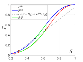
Figure 23: The orbit in the $S$-$F$ plane representing a stable saturation plateau for Scenario B. The equilibrium points for this orbit are shown on the flux curves.

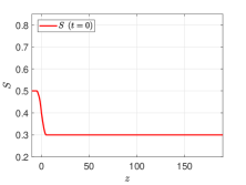
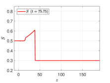
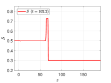
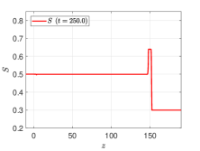
Figure 24: Saturation profiles for different time points. Besides the initial condition (top left) and the final saturation profile (bottom right), two intermediate profiles are shown, which have the form of a plateau. Contrary to the final saturation profile their plateaus are not stable, since the speeds of the infiltration and the drainage fronts are equal only for $S_{P}=0.634$.

6 Final remarks and comparison with experiments

In this work, a one-dimensional two-phase flow model has been analysed for infiltration problems. For simplicity, we have assumed that the medium is homogeneous and a constant total velocity is prescribed at the boundary. Dynamic and hysteretic effects are included in the capillary pressure with transitions between drainage and infiltration processes being modelled by a play-type hysteresis model having vertical scanning curves. Relative permeabilities are modelled as functions of saturation and capillary pressure in order to make their hysteretic nature explicit.

The focus being on travelling waves (TW), the system of partial differential equations is transformed into a dynamical system. This system is analysed for two different scenarios, A and B. In Scenario A, the hysteresis appears only in the capillary pressure, and we consider a broad range of dynamic capillarity terms, from small to large ones. In Scenario B, hysteresis is included in both the relative permeabilities and in the capillary pressure, whereas the dynamic capillary effects are kept small. For each scenario the existence of TW solutions is studied. In particular, we show that if the dynamic capillary effects exceed a certain threshold value, the TW profiles become non-monotonic. Such results complement the analysis in [18, 68, 43] done for the unsaturated flow case, respectively in [69, 67] for two-phase flow but without hysteresis. From practical point of view, the present analysis provides a criterion for the occurrence of overshoots in two-phase infiltration experiments.

Based on the TW analysis, we give admissibility conditions for shock solutions to the hyperbolic limit of the system. Motivated by the hysteretic and dynamic capillarity effects, such solutions do not satisfy the classical entropy condition. This is because the standard entropy solutions to hyperbolic two-phase flow models are obtained as limits of solutions to classical two-phase flow models, thus not including hysteresis and dynamic capillarity. In particular, for the infiltration case of Scenario A, apart from the classical solutions, there can be solutions consisting of (i) an infiltration shock followed by a rarefaction wave having non-matching speeds, or (ii) an infiltration shock followed by a drainage shock resulting in a growing saturation plateau (overshoot) in between. This is similar to the results in [69, 67]. In Scenario B, the entropy solutions are shown to depend also on the initial pressure. In particular, if certain parametric conditions are met, the solutions may include ones featuring a stable saturation plateau between an infiltration front and a drainage front, both travelling with the same velocity. Such solutions are obtained e.g. in [59], but only after generating the overshoot through a change in the boundary condition. All cases mentioned above have been reproduced by numerical experiments, in which a good resemblance has been observed between the TW results and the long time behaviour of the solutions to the original system of partial differential equations.

From practical point of view, we note that the present analysis can also be used to explain experimental results reported e.g. in [19, 33, 25, 72]. The occurrence of saturation overshoots is predicted theoretically for high enough dynamic capillary effects, namely of the $\tau$ value in (26). In dimensionless setting this can be assimilated to an injection rate that is sufficiently large. This is in line with the experimental results in [19], where the development of plateau like profiles was observed for high enough injection rates, as shown in Figure 5 of [19] and Figure 5.3 of [72]. Similarly, in the water and oil case, the plateaus are seen to develop and grow in Figures 5-6, 8-9, 18 of [24]. This behaviour is predicted by the analysis in Section 3. Moreover, Figure 10 of [24] might be presenting the case when the saturation has developed a plateau between two fronts travelling with the same velocity, a situation that is explained by the authors by means of hysteretic effects in the flux functions. Such solutions are investigated numerically in [59, 31], where it is shown that the plateaus can persist in time but without explaining how they are generated. The results in Section 4 partly support the conclusions there, but also explain the mechanism behind the development of such plateaus. We mention [32] in this regard, where the authors conclude that a similar mechanism must be responsible for observed stable saturation plateaus inside viscous fingers.

References

- [1] E. Abreu, A. Bustos, P. Ferraz, and W. Lambert. A relaxation projection analytical–numerical approach in hysteretic two-phase flows in porous media. Journal of Scientific Computing, pages 1–45, 2019.
- [2] J. Bear. Hydraulics of groundwater. McGraw-Hill International Book Co., 1979.
- [3] N. Bedjaoui and P.G. LeFloch. Diffusive–dispersive traveling waves and kinetic relations: Part i: Nonconvex hyperbolic conservation laws. Journal of Differential Equations, 178(2):574–607, 2002.
- [4] P. Bedrikovetsky, D. Marchesin, and P.R. Ballin. Mathematical model for immiscible displacement honouring hysteresis. In SPE Latin America/Caribbean Petroleum Engineering Conference. Society of Petroleum Engineers, 1996.
- [5] E.E. Behi-Gornostaeva, K. Mitra, and B. Schweizer. Traveling wave solutions for the richards equation with hysteresis. 2018.
- [6] A. Beliaev and S.M. Hassanizadeh. A theoretical model of hysteresis and dynamic effects in the capillary relation for two-phase flow in porous media. Transport in Porous media, 43(3):487–510, 2001.
- [7] M. Böhm and R.E. Showalter. Diffusion in fissured media. SIAM Journal on Mathematical Analysis, 16(3):500–509, 1985.
- [8] S. Bottero, S.M. Hassanizadeh, P.J. Kleingeld, and T.J. Heimovaara. Nonequilibrium capillarity effects in two-phase flow through porous media at different scales. Water Resources Research, 47(10), 2011.
- [9] E.M. Braun, R.F. Holland, et al. Relative permeability hysteresis: Laboratory measurements and a conceptual model. SPE Reservoir Engineering, 10(03):222–228, 1995.
- [10] M. Brokate, N.D. Botkin, and O.A. Pykhteev. Numerical simulation for a two-phase porous medium flow problem with rate independent hysteresis. Physica B: Condensed Matter, 407(9):1336–1339, 2012.
- [11] R.H. Brooks and A.T. Corey. Properties of porous media affecting fluid flow. Journal of the Irrigation and Drainage Division, 92(2):61–90, 1966.
- [12] G. Camps-Roach, D.M. O’Carroll, T.A. Newson, T. Sakaki, and T.H. Illangasekare. Experimental investigation of dynamic effects in capillary pressure: Grain size dependency and upscaling. Water Resources Research, 46(8), 2010.
- [13] X. Cao and K. Mitra. Error estimates for a mixed finite element discretization of a two-phase porous media flow model with dynamic capillarity. UHasselt Computational Mathematics Preprint Nr. UP-18, 2, 2018.
- [14] X. Cao, S.F. Nemadjieu, and I.S. Pop. Convergence of an MPFA finite volume scheme for a two-phase porous media flow model with dynamic capillarity. IMA Journal of Numerical Analysis, 2018.
- [15] X. Cao and I.S. Pop. Two-phase porous media flows with dynamic capillary effects and hysteresis: Uniqueness of weak solutions. Computers & Mathematics with Applications, 69(7):688 – 695, 2015.
- [16] X. Cao and I.S. Pop. Uniqueness of weak solutions for a pseudo-parabolic equation modeling two phase flow in porous media. Applied Mathematics Letters, 46:25–30, 2015.
- [17] X. Cao and I.S. Pop. Degenerate two-phase porous media flow model with dynamic capillarity. Journal of Differential Equations, 260(3):2418–2456, 2016.
- [18] C. Cuesta, C.J. van Duijn, and J. Hulshof. Infiltration in porous media with dynamic capillary pressure: travelling waves. European Journal of Applied Mathematics, 11(4):381–397, 2000.
- [19] D.A. DiCarlo. Experimental measurements of saturation overshoot on infiltration. Water Resources Research, 40(4), 2004.
- [20] C.J. van Duijn and K. Mitra. Hysteresis and horizontal redistribution in porous media. Transport in Porous Media, 122(2):375–399, Mar 2018.
- [21] A.G. Egorov, R.Z. Dautov, J.L. Nieber, and A.Y. Sheshukov. Stability analysis of gravity-driven infiltrating flow. Water resources research, 39(9), 2003.
- [22] G.A. El, M.A. Hoefer, and M. Shearer. Dispersive and diffusive-dispersive shock waves for nonconvex conservation laws. SIAM Review, 59(1):3–61, 2017.
- [23] R.E. Ewing. Time-stepping galerkin methods for nonlinear sobolev partial differential equations. SIAM Journal on Numerical Analysis, 15(6):1125–1150, 1978.
- [24] R.E. Gladfelter and S.P. Gupta. Effect of fractional flow hysteresis on recovery of tertiary oil. Society of Petroleum Engineers Journal, 20(06):508–520, 1980.
- [25] R.J. Glass, T.S. Steenhuis, and J.Y. Parlange. Mechanism for finger persistence in homogeneous, unsaturated, porous media: Theory and verification. Soil Science, 148(1):60–70, 1989.
- [26] M. Graf, M. Kunzinger, D. Mitrovic, and DJ. Vujadinovic. A vanishing dynamic capillarity limit equation with discontinuous flux. arXiv preprint arXiv:1805.02723, 2018.
- [27] S.M. Hassanizadeh and W.G. Gray. Mechanics and thermodynamics of multiphase flow in porous media including interphase boundaries. Advances in Water Resources, 13(4):169 – 186, 1990.
- [28] S.M. Hassanizadeh and W.G. Gray. Thermodynamic basis of capillary pressure in porous media. Water Resources Research, 29(10):3389–3405, 1993.
- [29] S.M. Hassanizadeh and W.G. Gray. Toward an improved description of the physics of two-phase flow. Advances in Water Resources, 16(1):53–67, 1993.
- [30] R. Helmig. Multiphase flow and transport processes in the subsurface: a contribution to the modeling of hydrosystems. Springer-Verlag, 1997.
- [31] R. Hilfer and R. Steinle. Saturation overshoot and hysteresis for twophase flow in porous media. European Physical Journal Special Topics, 223(11):2323–2338, 2014.
- [32] A.R. Kacimov and N.D. Yakimov. Nonmonotonic moisture profile as a solution of Richards’ equation for soils with conductivity hysteresis. Advances in Water Resources, 21(8):691–696, 1998.
- [33] F.J-M. Kalaydjian. Dynamic capillary pressure curve for water/oil displacement in porous media: Theory vs. experiment. In SPE Annual Technical Conference and Exhibition. Society of Petroleum Engineers, 1992.
- [34] S. Karpinski and I.S. Pop. Analysis of an interior penalty discontinuous galerkin scheme for two phase flow in porous media with dynamic capillary effects. Numerische Mathematik, 136(1):249–286, 2017.
- [35] S. Karpinski, I.S. Pop, and F.A. Radu. Analysis of a linearization scheme for an interior penalty discontinuous Galerkin method for two-phase flow in porous media with dynamic capillarity effects. International Journal for Numerical Methods in Engineering, 112(6):553–577, 2017.
- [36] J.E. Killough. Reservoir simulation with history-dependent saturation functions. Society of Petroleum Engineers Journal, 16(01):37–48, 1976.
- [37] P.G. LeFloch. Hyperbolic Systems of Conservation Laws: The theory of classical and nonclassical shock waves. Springer Science & Business Media, 2002.
- [38] M.C. Leverett. Capillary behavior in porous solids. Transactions of the AIME, 142(01):152–169, 1941.
- [39] F. List and F.A. Radu. A study on iterative methods for solving richards’ equation. Computational Geosciences, 20(2):341–353, 2016.
- [40] S. Manthey, S.M. Hassanizadeh, R. Helmig, and R. Hilfer. Dimensional analysis of two-phase flow including a rate-dependent capillary pressure–saturation relationship. Advances in water resources, 31(9):1137–1150, 2008.
- [41] A. Mikelić. A global existence result for the equations describing unsaturated flow in porous media with dynamic capillary pressure. Journal of Differential Equations, 248(6):1561–1577, 2010.
- [42] K. Mitra and I.S. Pop. A modified l-scheme to solve nonlinear diffusion problems. Computers & Mathematics with Applications, 77(6):1722 – 1738, 2019. 7th International Conference on Advanced Computational Methods in Engineering (ACOMEN 2017).
- [43] K. Mitra and C.J. van Duijn. Wetting fronts in unsaturated porous media: the combined case of hysteresis and dynamic capillary. 2018.
- [44] N. Morrow, C. Harris, et al. Capillary equilibrium in porous materials. Society of Petroleum Engineers Journal, 5(01):15–24, 1965.
- [45] Y. Mualem. A conceptual model of hysteresis. Water Resources Research, 10(3):514–520, 1974.
- [46] J. Niessner and S.M. Hassanizadeh. A model for two-phase flow in porous media including fluid-fluid interfacial area. Water Resources Research, 44(8), 2008.
- [47] O.A. Oleinik. Discontinuous solutions of non-linear differential equations. Uspekhi Matematicheskikh Nauk, 12(3):3–73, 1957.
- [48] A. Papafotiou, H. Sheta, and R. Helmig. Numerical modeling of two-phase hysteresis combined with an interface condition for heterogeneous porous media. Computational Geosciences, 14(2):273–287, 2010.
- [49] J.C. Parker, R.J. Lenhard, and T. Kuppusamy. A parametric model for constitutive properties governing multiphase flow in porous media. Water Resources Research, 23(4):618–624, 1987.
- [50] J.R. Philip. Similarity hypothesis for capillary hysteresis in porous materials. Journal of Geophysical Research, 69(8):1553–1562, 1964.
- [51] B. Plohr, D. Marchesin, P. Bedrikovetsky, and P. Krause. Modeling hysteresis in porous media flow via relaxation. Computational Geosciences, 5(3):225–256, 2001.
- [52] I.S. Pop, F.A. Radu, and P. Knabner. Mixed finite elements for the Richards equation: linearization procedure. Journal of Computational and Applied Mathematics, 168(1):365–373, 2004.
- [53] I.S. Pop, C.J. van Duijn, J. Niessner, and S.M. Hassanizadeh. Horizontal redistribution of fluids in a porous medium: The role of interfacial area in modeling hysteresis. Advances in Water Resources, 32(3):383–390, 2009.
- [54] A. Poulovassilis. Hysteresis of pore water in granular porous bodies. Soil Science, 109(1):5–12, 1970.
- [55] A. Rätz and B. Schweizer. Hysteresis models and gravity fingering in porous media. ZAMM-Journal of Applied Mathematics and Mechanics/Zeitschrift für Angewandte Mathematik und Mechanik, 94(7-8):645–654, 2014.
- [56] F. Rezanezhad, H-J. Vogel, and K. Roth. Experimental study of fingered flow through initially dry sand. Hydrology and Earth System Sciences Discussions, 3(4):2595–2620, 2006.
- [57] L.A. Richards. Capillary conduction of liquids through porous mediums. Physics, 1(5):318–333, 1931.
- [58] C.E. Schaerer, D. Marchesin, M. Sarkis, and P. Bedrikovetsky. Permeability hysteresis in gravity counterflow segregation. SIAM Journal on Applied Mathematics, 66(5):1512–1532, 2006.
- [59] M. Schneider, T. Köppl, R. Helmig, R. Steinle, and R. Hilfer. Stable propagation of saturation overshoots for two-phase flow in porous media. Transport in Porous Media, 121(3):621–641, 2018.
- [60] B. Schweizer. Laws for the capillary pressure in a deterministic model for fronts in porous media. SIAM Journal on Mathematical Analysis, 36(5):1489–1521, 2005.
- [61] B. Schweizer. Instability of gravity wetting fronts for Richards equations with hysteresis. Interfaces and Free Boundaries, 14(1):37–64, 2012.
- [62] B. Schweizer. The Richards equation with hysteresis and degenerate capillary pressure. Journal of Differential Equations, 252(10):5594 – 5612, 2012.
- [63] M. Shearer, K.R. Spayd, and E.R. Swanson. Traveling waves for conservation laws with cubic nonlinearity and bbm type dispersion. Journal of Differential Equations, 259(7):3216–3232, 2015.
- [64] S. Shiozawa and H. Fujimaki. Unexpected water content profiles under flux-limited one-dimensional downward infiltration in initially dry granular media. Water Resources Research, 40(7), 2004.
- [65] K. Spayd and M. Shearer. The Buckley–Leverett equation with dynamic capillary pressure. SIAM Journal on Applied Mathematics, 71(4):1088–1108, 2011.
- [66] G.C. Topp and E.E. Miller. Hysteretic moisture characteristics and hydraulic conductivities for glass-bead media. Soil Science Society of America Journal, 30(2):156–162, 1966.
- [67] C.J. van Duijn, Y. Fan, L.A. Peletier, and I.S. Pop. Travelling wave solutions for degenerate pseudo-parabolic equations modelling two-phase flow in porous media. Nonlinear Analysis: Real World Applications, 14(3):1361–1383, 2013.
- [68] C.J. van Duijn, K. Mitra, and I.S. Pop. Travelling wave solutions for the Richards equation incorporating non-equilibrium effects in the capillarity pressure. Nonlinear Analysis: Real World Applications, 41(Supplement C):232 – 268, 2018.
- [69] C.J. Van Duijn, L.A. Peletier, and I.S. Pop. A new class of entropy solutions of the Buckley–Leverett equation. SIAM Journal on Mathematical Analysis, 39(2):507–536, 2007.
- [70] C.J. Van Duijn, G.J.M. Pieters, and P.A.C. Raats. Steady flows in unsaturated soils are stable. Transport in Porous Media, 57(2):215–244, 2004.
- [71] H. Zhang and P.A. Zegeling. A numerical study of two-phase flow models with dynamic capillary pressure and hysteresis. Transport in Porous Media, 116(2):825–846, Jan 2017.
- [72] L. Zhuang. Advanced theories of water redistribution and infiltration in porous media: Experimental studies and modeling. PhD thesis, University of Utrecht, Dept. of Earth Sciences, 2017.
- [73] L. Zhuang, C.R. Bezerra Coelho, S.M. Hassanizadeh, and M.Th. van Genuchten. Analysis of the hysteretic hydraulic properties of unsaturated soil. Vadose Zone Journal, 16(5), 2017.