The Systematics of Galaxy Morphology in the Comprehensive de Vaucouleurs revised Hubble-Sandage Classification System: Application to the EFIGI Sample

Abstract

This paper is the third which examines galaxy morphology from the point of view of comprehensive de Vaucouleurs revised Hubble-Sandage (CVRHS) classification, a variation on the original de Vaucouleurs classification volume that accounts for finer details of galactic structure, including lenses, nuclear structures, embedded disks, boxy and disky components, and other features. The classification is applied to the EFIGI sample, a well-defined set of nearby galaxies which were previously examined by Baillard et al. and de Lapparent et al. The survey is focussed on statistics of features, and brings attention to exceptional examples of some morphologies, such as skewed bars, blue bar ansae, bar-outer pseudoring misalignment, extremely elongated inner SB rings, outer rings and lenses, and other features that are likely relevant to galactic secular evolution and internal dynamics. The possibility of using these classifications as a training set for automated classification algorithms is also discussed.

1 Introduction

Comprehensive galaxy morphology and classification refers to standard galaxy classification with more emphasis than usual on the fine details of galactic structure. Such an approach to morphology is warranted by theoretical progress in understanding galactic structure and evolution (Kormendy 2012), advances in the sophistication of numerical simulation models of galaxies (e.g., Dickinson et al. 2018; Eliche-Moral et al. 2018), and by the explosion of high quality, multi-wavelength images of nearby and very distant galaxies already available or coming in the near future (Domínguez Sánchez et al. 2019). After nearly a century since Hubble (1926) first published his ideas on galaxy morphology, galaxy classification is still an essential step in the study of the basic properties of galaxies and of cosmology and the structure of the Universe. As noted by Simmons et al. (2017), “Visual morphologies remain among the most nuanced and powerful measures of galaxy structure."

The large amount of high quality imaging available at this time makes it possible to take galaxy morphology and classification to realms it has not been taken before. Prior to the Sloan Digital Sky Survey (SDSS; Gunn et al. 1998, 2006; York et al. 2000), few galaxies had large-scale photographic plate images available for detailed morphological examination (Sandage & Bedke 1994). The majority of nearby galaxies had their morphological classifications judged instead from small-scale sky survey prints or plates (e.g., the Palomar Sky Survey, the ESO-$B$ sky survey, and the SRC-$J$ sky survey; de Vaucouleurs et al. 1991, hereafter RC3). The high quality of these surveys provided a rich source of morphological information, but the small-scale made it difficult to reliably classify some galaxies, especially early-type galaxies, and the details in the centers of many galaxies were lost to either overexposure or the contrast limits of photographic prints.

The SDSS provides enough new high quality image material to allow classification details to be seen in several hundred thousand galaxies. While an inventory of the types of these galaxies would be important for cosmological studies, the sheer number of objects makes visual classification by professional astronomers impractical. This led to the Galaxy Zoo project (Lintott et al. 2008), which drew volunteers from the general public to classify in a rudimentary way more than 300,000 SDSS galaxies (Willett et al. 2013). More recently, the Galaxy Zoo approach has been applied to more distant galaxies, including 48,000 galaxies in the CANDELS survey (Simmons et al. 2017) and 120,000 galaxies in archival Hubble Space Telescope imaging (Willett et al. 2017).

Several large professional morphological surveys of SDSS galaxies have been made. For example, Fukugita et al. (2007) classified 2253 SDSS galaxies in a simplified revised Hubble system; their final types are based on the independent classifications of three astronomers. Nair & Abraham (2010) used a more comprehensive approach, classifying 14,034 galaxies having 0.01 $<$ $z$ $<$ 0.1 in a system similar to RC3 and to the Revised Shapley-Ames catalog (Sandage and Tammann 1981; Sandage and Bedke 1994), and including additional features like lenses, tidal tails, and warps.

One of the largest efforts of multiple astronomers was made by Baillard et al. (2011), where a team of 10 professional astronomers classified subsets of 4458 RC3 galaxies for a survey titled “Extraction of the Idealized Forms of Galaxies in Images" (French acronym: EFIGI). The EFIGI sample was chosen to have many examples of all galaxy types, and the use of multiple classifiers allowed checks on personal classification equations and homogenization of the database. More recently, Ann et al. (2015) presented visual classifications of 5836 galaxies having $z$ $<$ 0.01. This sample includes many dwarf galaxies and complements other sources, such as Nair and Abraham (2010).

Modern morphological studies do not always involve application of classification symbolism as in the Hubble or de Vaucouleurs atlases of galaxies (e.g., classifications like SBb, SA(rs)a, etc.; Sandage 1961; Buta et al. 2007). Fukugita et al. (2007) only present modified numerical $T$-types and no information on other morphological features of their sample galaxies. Nair & Abraham (2010) use an RC3 coded approach for $T$-types, but for other features (bars, rings, lenses, etc.), a code based on a sum of powers of 2 was used rather than conventional letter symbolism. Baillard et al. (2011) classified the EFIGI sample using numerical codings of 16 visual “attributes", including apparent bulge-to-total luminosity ratio, properties of spiral arms, bars, rings, dust features, star-forming regions, and environmental characteristics. With these numerical codings and 10 classifiers, Baillard et al. were able to define an “EFIGI Hubble sequence" (EHS) and carry out a “morphometric" analysis of their sample. In each of these cases, the goal was not only to provide reliable morphological information on large numbers of nearby galaxies, but also to set up standards for facilitating automatic classification algorithms.

This paper is focussed on a re-examination of the EFIGI sample using the Comprehensive de Vaucouleurs revised Hubble-Sandage (CVRHS) classification system, in order to examine the systematics of morphology within the system. The CVRHS is a variation on the de Vaucouleurs (1959) classification volume that recognizes features of interest beyond the original system. The goals of the reclassification are: (1) to provide new classifications of EFIGI galaxies of a similar nature to RC3 classifications, but which supercede the latter and are useful for statistical studies; (2) to identify unusual or special objects that may shed light on galactic evolutionary processes; and (3) to help define the CVRHS as a point of view for further studies of galaxy morphology, including the facilitation of automated galaxy classification and its application to large samples of galaxies.

The CVRHS is briefly described in sections 2 and 3. The classification procedure is described in section 4, and both an internal and external comparison of classifications is described in section 5. The mean catalogue is described in section 6. Some statistics in the catalogue are examined in section 7. Finally, montages of special features of interest are provided in section 8.

2 CVRHS Morphological Classification

The CVRHS is a galaxy classification system tied to that of Hubble (1926; see also Sandage 1961) but as revised by de Vaucouleurs (1959), the latter also called the de Vaucouleurs revised Hubble-Sandage or VRHS system, which is the system used in RC3. Because of extensive continuing use of RC3 nearly 30 years after its publication, the VRHS is the “most applied" classification system in extragalactic studies, at least for nearby galaxies. The comprehensive element was added to the VRHS in several studies, but is most thoroughly described by Buta et al. (2015).

The CVRHS system has been most recently applied to two samples: the nearly 2400 galaxies in the Spitzer Survey of Stellar Structure in Galaxies (S⁴G; Sheth et al. 2010) by Buta et al. (2015), and to 3962 ringed galaxies drawn from the Galaxy Zoo 2 project (Willett et al. 2013; Buta 2017a). The historical waveband for galaxy classification is a blue-sensitive photographic emulsion, which neither of these studies used. The S⁴G classification used 3.6$\mu$m mid-infrared images in units of magnitudes per square arcsecond, while the ringed galaxy classification used SDSS color images (Lupton et al. 2004). For the EFIGI classification, SDSS $g$-band images (effective wavelength 477 nm) in units of magnitudes per square arcsecond are used. This also does not match the historical waveband for galaxy classification, but nevertheless is one of the closest modern approximations. Eskridge et al. (2002) discuss the systematic differences that can arise in galaxy classification when the old blue light systems are applied at a drastically different wavelength such as the infrared.

3 Scientific Advantages of CVRHS Classification

It is a fair question to ask what scientific advantages the CVRHS system might have over other approaches to galaxy classification. Consistent with the VRHS, the CVRHS provides more detailed morphological information than conventional Hubble types (e.g., Sandage 1961) without being too unwieldy. For most galaxies, a CVRHS type is little different from a VRHS type. Nevertheless, the detailed nature of CVRHS classification is ideal for interpreting SDSS images of relatively nearby galaxies, which is important because modern simulations (e.g., Illustris; Dickinson et al. 2018) have reached the point where model galaxies resemble real galaxies well enough that they can be compared to specific SDSS galaxies.

One advantage of CVRHS classification over others is the extent to which inner, outer, and nuclear varieties are recognized, These characteristics of galaxy morphology are important aspects of internal disk galaxy dynamics. For example, a significant part of CVRHS morphology involves the recognition of the different types of ring phenomena, including pseudorings and lenses, which have been tied to galactic secular evolutionary processes (Kormendy 1979; 2012). Although inner and outer rings are already recognized in the VRHS system, CVRHS morphology in addition recognizes nuclear rings, special subclasses of outer rings, as well as rare multiple inner, outer, and nuclear rings, pseudorings, and lenses. The R₁, R${}_{1}^{\prime}$, R${}_{2}^{\prime}$, and R₁R${}_{2}^{\prime}$ subclasses of outer rings and pseudorings (Buta and Crocker 1991) are an example of CVRHS features that can be tied to specific aspects of internal dynamics, such as resonant (Buta and Combes 1996) or manifold (Athanassoula et al. 2010 and references therein) dynamics.

It is also fair to ask whether and how CVRHS classification facilitates the identification of rare or special objects. While special cases could of course be noted without appealing to CVRHS morphology, the CVRHS provides a better context for recognizing such cases because the level of detail demands a close inspection of the features defining the classification. Also, when applying the CVRHS to a sample, every galaxy is viewed in the context of the whole, which makes special cases stand out. Finally, any classification allows the drawing of samples for further study, and the more detailed the classification, the more specific a sample can be.

4 CVRHS Classification of EFIGI Galaxies

The EFIGI sample was chosen for this study because the sample was carefully selected by Baillard et al. (2011) to include mainly galaxies having a reliable RC3 classification; the sample is large enough to have many examples of each galaxy type, but small enough to allow CVRHS classification by a single person in a reasonable amount of time; and the authors posted on a public website (www.astromatic.net/projects/efigi) the full set of color images and individual filter images they used for their study, making it possible to focus entirely on morphology and not on image preparation. De Lapparent et al. (2011) summarize other statistics of the EFIGI catalogue. Redshifts range from nearly 0 to 0.07, absolute $g$-band magnitudes range from $-$13 to $-23$, and linear diameters range from 1-100 kpc.

The CVRHS classification of the EFIGI sample is based on logarithmic, background-subtracted SDSS images converted to units of magnitudes per square arcsecond. This is the display system of the de Vaucouleurs Atlas of Galaxies (deVA, Buta et al. 2007). The images are from Data Release 4 (Adelman-McCarthy et al. 2006), and all such images have known zero points in the $AB$ magnitude system. The typical zero point in the $g$-band is 26.5 mag arcsec^-2, which allowed a homogeneous display of all of the galaxies. The conversion of units to mag arcsec^-2 is essential to CVRHS morphology as applied in the deVA, although an actual zero point is not a stringent requirement.

The classification of the EFIGI galaxies was carried out in three phases: Phase 1 (2012) and Phase 2 (2017) involved independent classifications of the full sample of 4458 galaxies, while phase 3 (2018) involved only 2019 spirals approximately in the stage range S0/a to Sd. The reason for such an approach is that multiple, independent examinations of the database of images allow internal consistency checks of the morphological interpretations. This is important because an observer may not view a galaxy in exactly the same manner from one examination to another, and combining multiple phases can improve the final classification.

The multi-phase approach to galaxy classification is an important part of this study, and its successful application depends on how well the different phases can be combined. For this purpose, several steps were used: (1) averaging the stage (E, S0, S, I); (2) averaging the family (SA, SAB, SB); (3) averaging the main part of the inner variety (r, rs, s, rl, l); (4) selecting the remaining parts of the inner variety; and (5) selecting the outer variety. For stage, family, and inner variety, the phases were combined using a numerical coding system. For stage, the coding system was the familiar $T$-index used in RC3, which ranges from $T$=$-$5 for E galaxies to $T$=10 for Im galaxies. For family, a modified coding scheme was used: $F$=0 for SA galaxies, 1 for S$\underline{\rm A}$B galaxies, 2 for SAB galaxies, 3 for SA$\underline{\rm B}$ galaxies, and 4 for SB galaxies. For inner variety, $IV$=0 for (s), 1 for (r$\underline{\rm s}$), 2 for (rs). 3 for $\underline{\rm r}$s), 4 for (r), 5 for (), 6 for (rl), 7 for (r$\underline{\rm l}$), and 8 for (l). The underline categories S$\underline{\rm A}$B, SA$\underline{\rm B}$, ($\underline{\rm r}$s), (r$\underline{\rm s}$) (de Vaucouleurs 1963) are directly applied in family and inner variety classifications in each phase. However, underline stages (e.g., S$\underline{\rm a}$b, Sb$\underline{\rm c}$, etc.) appear only in the averaged classifications.

5 Comparison of Classifications

5.1 Internal Consistency

Figure 1 shows how well the stage, family, and inner variety classifications from the three phases agree. Each stage graph plots two sets of points: $<T_{j}>$ versus $T_{i}$ and $T_{j}$ versus $<T_{i}>$, for phases $i$ and $j$; each family graph plots $<F_{j}>$ versus $F_{i}$ and $F_{j}$ versus $<F_{i}>$; and each inner variety graph plots $<IV_{j}>$ versus $IV_{i}$ and $IV_{j}$ versus $<IV_{i}>$. The error bars in each direction are 1$\sigma$ standard deviations. In general, the agreement between stage, family, and inner variety classifications from the three phases is good. Table 1 shows that of 2019 galaxies having three independent classifications, 120 (or 5.9%) received an identical full classification in all three phases, while out of 4458 galaxies, 952 (21.4%) received two identical full classifications. For more than half the sample, the same stage, family, or variety was assigned ($|\Delta T|$, $|\Delta F|$, or $|\Delta(IV)|$ =0). A small percentage have $|\Delta T|$, $|\Delta F|$, or $|\Delta(IV)|$ $>$3; such large discrepancies are often associated with complex objects difficult to fit into the classification system.

Table 2 summarizes the results of an analysis of the internal dispersions in the assignments of CVRHS stage, family, and inner variety classifications for EFIGI galaxies. In general, systematic differences in these attributes for the different phases are small. The dispersions are derived from

$$\sigma_{ij}^{2}={1\over N}\Sigma(T_{i}-T_{j})^{2}$$ (1)

for phases $i$ and $j$, where $N$ is the total number of galaxies in the comparison. From these combined dispersions, the individual $\sigma_{i}$ can be derived using linear least squares. The results are given in terms of intervals: for example, 1 stage interval is a difference such as Sab to Sb; 1 family interval is a difference such as SA to S$\underline{\rm A}$B; and 1 inner variety interval is a difference such as ($\underline{\rm r}$s) to (r). The analysis is restricted to spirals because only spirals in the range S0/a to Sd (based on an initial average of phase 1 and 2 classifications) have classifications in all three phases. There is an indication that Phase 2 and 3 classifications are more internally consistent than are phase 1 classifications. For example, $\sigma_{1}(F)$ = 0.76 while $\sigma_{2}(F)$ = 0.52 and $\sigma_{3}(F)$ = 0.57. Such differences are not likely to be significant, and Table 2 adopts the averages $<\sigma_{i}(T)>$ = 0.7 stage intervals, $<\sigma_{i}(F)$> = 0.6 family intervals, and $<\sigma_{i}(IV)>$ = 1.1 inner variety intervals. These dispersions are characteristic of the classifications for a single phase, but if $n$ phases are averaged, then the internal dispersion is derived as $<\sigma_{i}>$/$\sqrt{n}$.

Figure 1: Comparison of stage, family, and inner variety classifications between Phases 1, 2, and 3

Table 1: Internal comparison of classifications

Comparison	$n_{12}$	% $N$	$n_{13}$	% $N$	$n_{23}$	% $N$
3 identical	120	5.9
$N$	2019
2 identical	952	21.4
$N$	4458
$\Delta T$=0	2283	52.5	1119	56.3	1179	59.3
$|\Delta T|$=1	1437	33.0	716	36.0	679	34.2
$|\Delta T|$=2	405	9.3	111	5.6	104	5.2
$|\Delta T|$=3	145	3.3	26	1.3	12	0.6
$|\Delta T|>$3	81	1.9	17	0.9	13	0.7
$N$	4351		1989		1987
$\Delta F$=0	1977	65.2	1249	63.0	1365	68.8
$|\Delta F|$=1	568	18.7	452	22.8	446	22.5
$|\Delta F|$=2	442	14.6	254	12.8	162	8.2
$|\Delta F|$=3	25	0.8	19	1.0	8	0.4
$|\Delta F|>$3	21	0.7	9	0.5	2	0.1
$N$	3033		1983		1983
$\Delta IV$=0	1751	70.4	1219	68.5	1252	67.6
$|\Delta IV|$=1	395	15.9	321	18.0	371	20.0
$|\Delta IV|$=2	316	12.7	219	12.3	212	11.4
$|\Delta IV|$=3	21	0.8	19	1.1	14	0.8
$|\Delta IV|>$3	3	0.1	2	0.1	4	0.2
$N$	2486		1780		1853

Table 2: Internal Agreement between stage and family classifications in Phases 1, 2, and 3. Each column gives the rms dispersion between the two phases ($i$ and $j$) indicated. The numbers in parentheses next to each value are the mean difference ($<T_{i}-T_{j}>$, $<F_{i}-F_{j}>$, or $<IV_{i}-IV_{j}>$) and the number of galaxies in the comparison. The individual $\sigma_{i}$ are derived from a linear least squares analysis.

$i\rightarrow$	1	2	3
$j$
$\downarrow$
		Stage
2	1.21(0.15,1984)	……….	……….
3	1.02($-$0.01,1989)	0.93($-$0.16,1987)	……….
$\sigma_{i}(T)$	0.90	0.80	0.47
$<\sigma_{i}(T)>$	0.7
		Family
2	0.92(0.20,1973)	……….	……….
3	0.95(0.26,1983)	0.78(0.06,1983)	……….
$\sigma_{i}(F)$	0.76	0.52	0.57
$<\sigma_{i}(F)>$	0.6
		Inner Variety
2	1.57(0.05,1894)	……….	……….
3	1.59(0.10,1905)	1.36(0.06,1933)	……….
$\sigma_{i}(IV)$	1.25	0.95	0.98
$<\sigma_{i}(V)>$	1.1

5.2 External Comparisons

External comparisons between the CVRHS types and published types from other sources are presented in Figures  2 and  3. Four external sources are examined: Baillard et al. (2011, source "EFIGI"), de Vaucouleurs et al. (1991, source "RC3"), Nair and Abraham (2010; source "NA"), and Ann et al. (2015, source "ASH"). Only stage and family classifications are compared (ASH do not judge inner or outer varieties). The line in each frame is for reference only and not a linear fit.

For the purposes of the comparison, mean stages ($<T>$) and mean families ($<F>$) were derived as unweighted averages of phases 1-3 for spirals and phases 1-2 for the remaining types. NA family classifications are specified by numbers $F$ = 2ⁱ, where $i$ = 1 for a strong bar, 2 for an intermediate bar, and 3 for a weak bar, and $F$=0 for no bar. In Figure 3, these are translated into classifications SB, SA$\underline{\rm B}$, SAB, and SA, respectively. NA noted that their bar classifications mainly emphasized strong bars.

Figure 2 shows good agreement between $<T>$ and the EFIGI Hubble sequence $T_{EFIGI}$ for types ranging from $T$ = $-$5 to $T$ = 10. Agreement with the other sources is good as well. Comparison between family classifications shows some systematic disagreements (e.g., $<F>$ is stronger on average than $F_{EFIGI}$ and $F_{NA}$, but weaker on average than $F_{RC3}$).

This is quantified further in Table 3, again using equation 1 and linear least squares. The five sources [this paper (RB), EFIGI, RC3, NA, and ASH) could not be used together since there is little or no overlap between NA and ASH. Only the galaxies in common with all of the available sources are used for this analysis. Table 3 presents separate analyses of sources RB, EFIGI, RC3, and NA, and then RB, EFIGI, RC3, and ASH. The average external dispersion for the modern sources is $<\sigma_{e}(T)>$ = 1.1 stage intervals, while that for RC3 is $<\sigma_{e}(T)>$ = 1.5 stage intervals. For family, the two sets do not give very consistent results for sources EFIGI and RC3. The average of the modern sources is $<\sigma_{e}(F)>$ = 0.8 family intervals while for RC3 it is $<\sigma_{e}(F)>$ = 1.5 family intervals. The results of both the internal and external comparisons are consistent with Buta et al. (2015) and Naim et al. (1995).

Figure 2: Comparison of Table 1 mean stage classifications with stage classifications from other sources: $T_{EFIGI}$ from Baillard et al. (2011; 4386 galaxies), $T_{RC3}$ from de Vaucouleurs et al. (1991; 4420 galaxies), $T_{NA}$ from Nair & Abraham (2010; 1389 galaxies), and $T_{ASH}$ from Ann et al. (2015; 1250 galaxies.)

Figure 3: Comparison of Table 1 mean family classifications with family classifications from other sources: $F_{EFIGI}$ from Baillard et al. (2011; 3319 galaxies), $F_{RC3}$ from de Vaucouleurs et al. (1991; 1884 galaxies), $F_{NA}$ from Nair & Abraham (2010;1158 galaxies), and $F_{ASH}$ from Ann et al. (2015; 715 galaxies)

Table 3: External Agreement Between Classifications. Each column gives the rms dispersion between the two sources ($i$ and $j$) indicated. The number in parentheses next to each value is the mean difference $<T_{i}-T_{j}>$. The individual $\sigma_{i}$ are derived from a linear least squares analysis. Sources: EFIGI=Baillard et al. (2011); NA2010=Nair & Abraham (2010); RC3=de Vaucouleurs et al. (1991); ASH = Ann et al. (2015)

Source	RB	EFIGI	RC3	NA
$i\rightarrow$	1	2	3	4
$j$
$\downarrow$
2	1.33(0.24)	……….	……….	……….
3	1.71(0.02)	1.80($-$0.228)	……….	……….
4	1.40(0.22)	1.64($-$0.02)	1.90(0.20)	……….
$\sigma_{i}(T)$	0.80	1.07	1.48	1.19
$N$=1389
Source	RB	EFIGI	RC3	ASH
$i\rightarrow$	1	2	3	4
$j$
$\downarrow$
2	1.56(0.15)	……….	……….	……….
3	1.88($-$0.22)	2.03($-$0.37)	……….	……….
4	1.73($-$0.32)	1.72($-$0.47)	1.68($-$0.10)	……….
$\sigma_{i}(T)$	1.15	1.27	1.44	1.12
$N$=1217
Source	RB	EFIGI	RC3	NA
$i\rightarrow$	1	2	3	4
$j$
$\downarrow$
2	0.99($-$0.46)	……….	……….	……….
3	1.71(0.85)	1.95(1.30)	……….	……….
4	1.17($-$0.57)	0.93($-$0.11)	2.14($-$1.41)	……….
$\sigma_{i}(F)$	0.46	0.63	1.80	1.00
$N$=628
Source	RB	EFIGI	RC3	ASH
$i\rightarrow$	1	2	3	4
$j$
$\downarrow$
2	1.40($-$0.89)	……….	……….	……….
3	1.41(0.50)	1.94(1.39)	……….	……….
4	1.14(0.19)	1.60(1.08)	1.36($-$0.31)	……….
$\sigma_{i}(F)$	0.62	1.38	1.25	0.79
$N$=504

6 Mean Catalogue

Table 4 presents the mean CVRHS classifications for the 4458 EFIGI sample galaxies (followed by notes for three-quarters of the sample). The galaxies are listed by Principal Galaxy Catalogue (PGC, Paturel et al. 1989) number, but most also have an alternate name that can take precedence over the PGC number. The names in column 1 are formal “NED names," i. e., the names adopted in the NASA/IPAC Extragalactic Database and were taken from a cross index provided on the EFIGI website. The radial velocity listed in column 3 is also from this cross index list. Column 4 lists the arm class (Elmegreen and Elmegreen 1987) for those galaxies where the image resolution and inclination allowed a judgment to be made. Columns 5 and 6 list numerical codes for the mean stage and family classifications. The $T$-type codes are the same as defined in RC3 with the exception that $T$=11 is used for dwarf elliptical, S0, and spheroidal galaxies. This is consistent with what Baillard et al. (2011) used for these same types. The coding for bar classification: $F$ = 0, 1, 2, 3, and 4 for types SA, S$\underline{\rm A}$B, SAB, SA$\underline{\rm B}$, and SB, respectively, is the same scale that Baillard et al. (2011) used, multiplied by a factor of 4. Column 7 lists the number of phases used for the averages. The final mean letter classification is listed in column 8.

Table 4: CVRHS Classifications for 4458 EFIGI Galaxies: Col. 1: name adopted in NASA/IPAC Extragalactic Database (NED); col. 2: number in Principal Galaxy Catalogue (Paturel et al. 1989); col. 3: heliocentric radial velocity from NED; col. 4: arm class (as defined by Elmegreen and Elmegreen 1987); col. 5: mean stage index on the RC3 scale; col. 6: mean family index on the scale used in this paper; col. 7: number of phases used for $<T>$ and $<F>$; col. 8: the average classification using CVRHS notation. (See Buta et al. 2015 for the meaning of different CVRHS symbols; the full table will be made available online).

NED Name	PGC	$V_{\odot}$	AC	$<T>$	$<F>$	$n$	Type
		km s-1
1	2	3	4	5	6	7	8
IC 5381	212	11231		2.5$\pm$0.7	1.0$\pm$1.1	2	S$\underline{\rm A}$Bx($\underline{\rm r}$s)a$\underline{\rm b}$  spw
NGC 7814	218	1050		1.0$\pm$0.5		2	Sa sp / E(d)5
NGC 7808	243	8787		0.0$\pm$0.4	0.0$\pm$0.3	3	SA()0/a
UGC 17	255	878	4	9.0$\pm$0.5	2.0$\pm$0.4	2	SAB(s)m
MCG $-$02-01-015	281	11491		5.0$\pm$4.0	3.0$\pm$1.1	2	SA$\underline{\rm B}$a(s)c pec

7 Distribution of Morphologies in the CVRHS-EFIGI Catalogue

Figures 4– 7 and Tables 5- 8 show distributions of classifications from the mean catalogue, for two samples in each case: a full, unrestricted sample, and a second sample restricted to RC3 isophotal axis ratio log$R_{25}$ $\leq$ 0.40. The latter restriction is meant to exclude galaxies more highly inclined than 66^o. The distribution of stages is comparable to what Baillard et al. (2011, their Figure 26) found, except that E and Im galaxies stand out more in part because the histograms in Figure 4 are plotted in half stage intervals rather than full stage intervals.

In both the full and restricted subsets in Table 5, Sb to Sc are the stages with the highest relative frequencies, with galaxies in the range Sa$\underline{\rm b}$ to S$\underline{\rm c}$d constituting 36-37% of the samples. The shape of the distribution of types is different from that expected for a distance-limited sample, which would tend to emphasize extreme late-type spirals and magellanic irregulars (e.g., Buta et al. 2015, their Figure 5; also Buta et al. 1994, their Figure 6). It is also different from a magnitude-limited sample, which would tend to de-emphasize such galaxies. Instead, the distributions are characteristic of an angular diameter-limited sample, as noted by de Lapparent et al. (2011; see also Buta et al 1994, their Figure 5).

The statistics of bar classifications shows that family SA has the highest relative frequency, constituting 33% of both the full and restricted samples. This means the EFIGI sample as classified according to the CVRHS system has a bar fraction of 67% if the weakest bars (type S$\underline{\rm A}$B) are included, or 53% based only on SAB, SA$\underline{\rm B}$, and SB types. The bar classifications in Table 4 are not defined in the same manner as the Baillard et al. (2011) bar attribute. CVRHS bar classifications account for bar length, axis ratio, and contrast, while the Baillard et al. (2011) bar attribute is based mainly on relative bar length.

Figure 6 and Table 7 show the CVRHS EFIGI bar fraction as a function of stage. Both the full and restricted samples show a significant minimum in bar frequency around stage Sc, with a lesser minimum at stage S0/a. The graphs also show that the bar fraction for stages Scd and later is greater than 80%, compared to $\approx$60% for stages S0⁺ to Sb. These trends are similar to what Buta et al. (2015) found for the S⁴G sample except that the minimum in the mid-IR occurs at a slightly earlier stage than Sc. The implication of this minimum is that conventional Sc galaxies rarely appear barred. In fact, one of the most common types in the catalogue is SA(s)c. Buta et al. (2015) also show that RC3 classifications show a minimum in bar fraction near stage Sc, although this minimum is much less significant.

Figure 4: Distribution of CVRHS Stages

Table 5: Statistics of Stages

$T$	$n$	%$N$	$T$	$n$	%$N$
1	2	3	1	2	3
		Full Sample	$N$=4429
$-$6.0	6	0.1	3.0	249	5.6
$-$5.5	4	0.1	3.5	252	5.7
$-$5.0	254	5.7	4.0	211	4.8
$-$4.5	77	1.7	4.5	280	6.3
$-$4.0	60	1.4	5.0	289	6.5
$-$3.5	23	0.5	5.5	205	4.6
$-$3.0	119	2.7	6.0	128	2.9
$-$2.5	54	1.2	6.5	178	4.0
$-$2.0	82	1.9	7.0	207	4.7
$-$1.5	67	1.5	7.5	134	3.0
$-$1.0	112	2.5	8.0	130	2.9
$-$0.5	61	1.4	8.5	115	2.6
0.0	84	1.9	9.0	133	3.0
0.5	100	2.3	9.5	76	1.7
1.0	129	2.9	10.0	203	4.6
1.5	117	2.6	10.5	6	0.1
2.0	105	2.4	11.0	30	0.7
2.5	149	3.4	….	…	…
		$logR_{25}$ $\leq$ 0.40	$N$=3018
$-$6.0	2	0.1	3.0	142	4.7
$-$5.5	2	0.1	3.5	173	5.7
$-$5.0	224	7.4	4.0	144	4.8
$-$4.5	66	2.2	4.5	209	6.9
$-$4.0	50	1.7	5.0	184	6.1
$-$3.5	20	0.7	5.5	138	4.6
$-$3.0	81	2.7	6.0	74	2.5
$-$2.5	35	1.2	6.5	117	3.9
$-$2.0	61	2.0	7.0	104	3.4
$-$1.5	43	1.4	7.5	72	2.4
$-$1.0	77	2.6	8.0	89	2.9
$-$0.5	34	1.1	8.5	67	2.2
0.0	59	2.0	9.0	97	3.2
0.5	66	2.2	9.5	51	1.7
1.0	92	3.0	10.0	158	5.2
1.5	79	2.6	10.5	4	0.1
2.0	67	2.2	11.0	30	1.0
2.5	109	3.6	….	…	…

Figure 5: Distribution of CVRHS Families

Table 6: Statistics of Families

Family	$F$	$n$	%$N$
1	2	3	4
	Full Sample	$N$=3416
SA	0.0	1140	33.4$\pm$0.8
S$\underline{\rm A}$B	1.0	462	13.5$\pm$0.6
SAB	2.0	658	19.3$\pm$0.7
SA$\underline{\rm B}$	3.0	422	12.4$\pm$0.6
SB	4.0	734	21.5$\pm$0.7
	$logR_{25}$ $\leq$ 0.40	$N$=2440
SA	0.0	812	33.3$\pm$1.0
S$\underline{\rm A}$B	1.0	321	13.2$\pm$0.7
SAB	2.0	460	18.9$\pm$0.8
SA$\underline{\rm B}$	3.0	296	12.1$\pm$0.7
SB	4.0	551	22.6$\pm$0.8

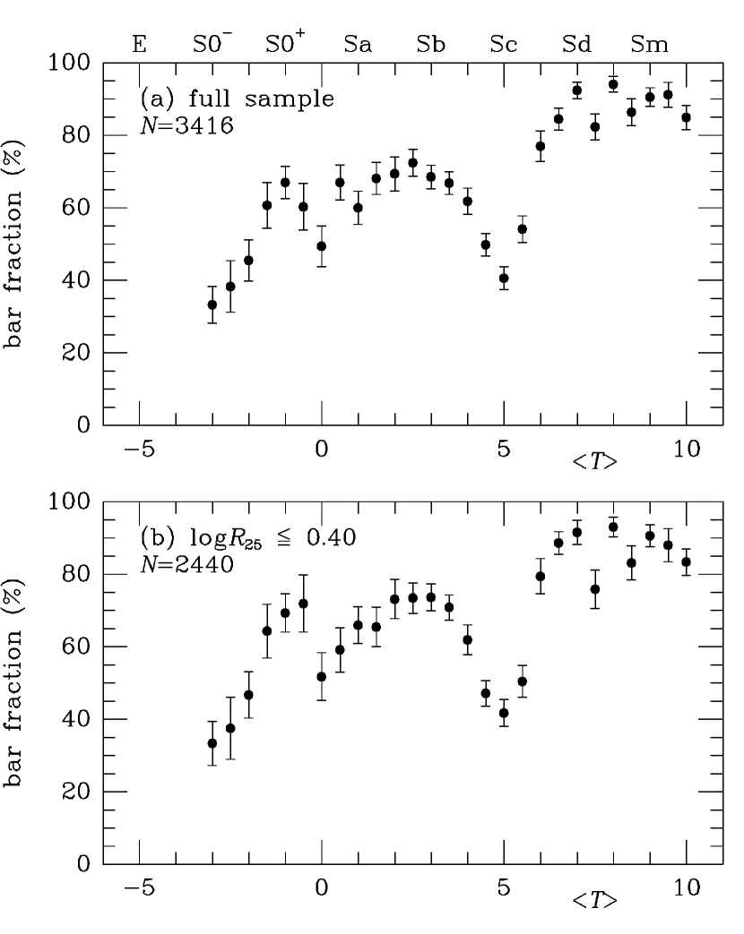
Figure 6: Bar fraction as a function of CVRHS stage

Table 7: Bar fraction versus stage

$T$	$f_{bar}$(%)	$N(T)$	$T$	$f_{bar}$(%)	$N(T)$
1	2	3	1	2	3
	Full Sample	$N$=3416
$-$3.0	33.3$\pm$5.1	84	4.0	61.8$\pm$ 3.6	186
$-$2.5	38.3$\pm$7.1	47	4.5	49.8$\pm$ 3.1	259
$-$2.0	45.5$\pm$5.7	77	5.0	40.6$\pm$ 3.1	244
$-$1.5	60.7$\pm$6.3	61	5.5	54.1$\pm$ 3.7	181
$-$1.0	67.0$\pm$4.5	109	6.0	77.0$\pm$ 4.2	100
$-$0.5	60.3$\pm$6.4	58	6.5	84.5$\pm$ 3.0	148
0.0	49.4$\pm$5.6	79	7.0	92.4$\pm$ 2.3	132
0.5	67.0$\pm$4.8	97	7.5	82.3$\pm$ 3.6	113
1.0	60.0$\pm$4.6	115	8.0	94.1$\pm$ 2.2	118
1.5	68.1$\pm$4.4	113	8.5	86.4$\pm$ 3.7	88
2.0	69.4$\pm$4.7	98	9.0	90.5$\pm$ 2.6	126
2.5	72.4$\pm$3.7	145	9.5	91.2$\pm$ 3.4	68
3.0	68.5$\pm$3.2	216	10.0	84.9$\pm$ 3.3	119
3.5	66.8$\pm$3.1	235	all $T$	66.6$\pm$ 0.8	3416
	$logR_{25}$ $\leq$ 0.40	$N$=2440
$-$3.0	33.3$\pm$6.1	60	4.0	61.9$\pm$ 4.1	139
$-$2.5	37.5$\pm$8.6	32	4.5	47.1$\pm$ 3.5	208
$-$2.0	46.7$\pm$6.4	60	5.0	41.7$\pm$ 3.7	175
$-$1.5	64.3$\pm$7.4	42	5.5	50.4$\pm$ 4.4	131
$-$1.0	69.3$\pm$5.3	75	6.0	79.4$\pm$ 4.9	68
$-$0.5	71.9$\pm$7.9	32	6.5	88.6$\pm$ 3.1	105
0.0	51.7$\pm$6.6	58	7.0	91.5$\pm$ 3.3	71
0.5	59.1$\pm$6.1	66	7.5	75.8$\pm$ 5.3	66
1.0	65.9$\pm$5.1	88	8.0	93.0$\pm$ 2.7	86
1.5	65.4$\pm$5.4	78	8.5	83.1$\pm$ 4.7	65
2.0	73.1$\pm$5.4	67	9.0	90.6$\pm$ 3.0	96
2.5	73.4$\pm$4.2	109	9.5	88.0$\pm$ 4.6	50
3.0	73.6$\pm$3.7	140	10.0	83.3$\pm$ 3.7	102
3.5	70.8$\pm$3.5	171	all $T$	66.7$\pm$ 1.0	2440

Figures 7– 9 and Tables 8– 11 show the statistics of CVRHS inner varieties grouped into three categories: inner rings and pseudorings [(rs), ($\underline{\rm r}$s), and (r)]; pure spirals and weak inner pseudorings [(s) and (r$\underline{\rm s}$)], and lenses and ring/pseudoring-lenses [($\underline{\rm r}$l), (rl), r$\underline{\rm l}$), (l), and (r^′l)]. Figure 7 shows that the most common inner variety is (s), and that inner pseudorings are more common than closed inner rings and ring-lenses. Figure 8 shows the relative frequency of the three inner variety subgroups versus CVRHS stage, which highlights how the most prominent inner rings and pseudorings occur near stage Sab (see also de Lapparent et al. 2011), and that the frequency of such rings declines rapidly towards earlier and later stages. (s) and (r$\underline{\rm s}$) varieties become most frequent for stages Sbc and later, while lenses and ring/pseudoring lenses are most common among S0s and become infrequent by stage S$\underline{\rm b}$c. Figure 9 shows the distribution of inner varieties by CVRHS family. These graphs show that although inner rings and well-defined inner pseudorings are most abundant in SB galaxies and least abundant in SA galaxies, there is still a significant ring frequency in SA galaxies. As for the bar fraction statistics, these trends also have little dependence on whether the sample used is the full sample or the restricted subset.

Figure 7: Distribution of CVRHS inner varieties

Table 8: Statistics of Inner Varieties

Inner Variety	$n$	%$N$
1	2	3
	Full Sample	$N$=3162
s	1515	47.9$\pm$ 0.9
r$\underline{\rm s}$	408	12.9$\pm$ 0.6
rs	458	14.5$\pm$ 0.6
$\underline{\rm r}$s	263	8.3$\pm$ 0.5
r	184	5.8$\pm$ 0.4
\lx@column@trimright	50	1.6$\pm$ 0.2
rl	33	1.0$\pm$ 0.2
r$\underline{\rm l}$	39	1.2$\pm$ 0.2
l	157	5.0$\pm$ 0.4
r′l	55	1.7$\pm$ 0.2
	$logR_{25}$ $\leq$ 0.40	$N$=2318
s	982	42.4$\pm$ 1.0
r$\underline{\rm s}$	327	14.1$\pm$ 0.7
rs	391	16.9$\pm$ 0.8
$\underline{\rm r}$s	224	9.7$\pm$ 0.6
r	134	5.8$\pm$ 0.5
\lx@column@trimright	43	1.9$\pm$ 0.3
rl	19	0.8$\pm$ 0.2
r$\underline{\rm l}$	32	1.4$\pm$ 0.2
l	119	5.1$\pm$ 0.5
r′l	47	2.0$\pm$ 0.3

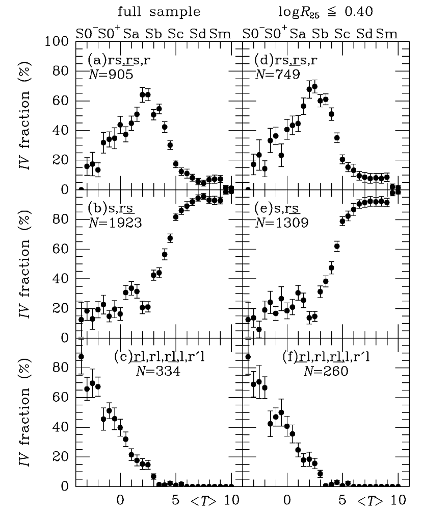
Figure 8: Distribution of CVRHS inner varieties versus stage. The numbers of objects in each subtype are listed in Table  8

Table 9: Statistics of Inner Varieties by stage - full sample

$T$	$n$	rs,$\underline{\rm r}$s,r	s,r$\underline{\rm s}$	,rl,r$\underline{\rm l}$,l,r′l
		$f$%	$f$%	$f$%
1	2	3	4	5
$-$3.5	8	0.0$\pm$ 0.0	12.5$\pm$11.7	87.5$\pm$11.7
$-$3.0	38	15.8$\pm$ 5.9	18.4$\pm$ 6.3	65.8$\pm$ 7.7
$-$2.5	23	17.4$\pm$ 7.9	13.0$\pm$ 7.0	69.6$\pm$ 9.6
$-$2.0	52	13.5$\pm$ 4.7	19.2$\pm$ 5.5	67.3$\pm$ 6.5
$-$1.5	44	31.8$\pm$ 7.0	22.7$\pm$ 6.3	45.5$\pm$ 7.5
$-$1.0	88	34.1$\pm$ 5.1	14.8$\pm$ 3.8	51.1$\pm$ 5.3
$-$0.5	46	34.8$\pm$ 7.0	19.6$\pm$ 5.8	45.7$\pm$ 7.3
0.0	73	43.8$\pm$ 5.8	16.4$\pm$ 4.3	39.7$\pm$ 5.7
0.5	91	37.4$\pm$ 5.1	30.8$\pm$ 4.8	31.9$\pm$ 4.9
1.0	107	44.9$\pm$ 4.8	33.6$\pm$ 4.6	21.5$\pm$ 4.0
1.5	108	50.9$\pm$ 4.8	31.5$\pm$ 4.5	17.6$\pm$ 3.7
2.0	92	64.1$\pm$ 5.0	20.7$\pm$ 4.2	15.2$\pm$ 3.7
2.5	142	64.1$\pm$ 4.0	21.1$\pm$ 3.4	14.8$\pm$ 3.0
3.0	205	50.7$\pm$ 3.5	42.4$\pm$ 3.5	6.8$\pm$ 1.8
3.5	229	54.6$\pm$ 3.3	44.1$\pm$ 3.3	1.3$\pm$ 0.8
4.0	184	42.4$\pm$ 3.6	56.5$\pm$ 3.7	1.1$\pm$ 0.8
4.5	258	30.2$\pm$ 2.9	67.4$\pm$ 2.9	2.3$\pm$ 0.9
5.0	240	17.5$\pm$ 2.5	81.7$\pm$ 2.5	0.8$\pm$ 0.6
5.5	178	12.4$\pm$ 2.5	86.0$\pm$ 2.6	1.7$\pm$ 1.0
6.0	100	11.0$\pm$ 3.1	89.0$\pm$ 3.1	0.0$\pm$ 0.0
6.5	146	8.2$\pm$ 2.3	91.8$\pm$ 2.3	0.0$\pm$ 0.0
7.0	125	5.6$\pm$ 2.1	94.4$\pm$ 2.1	0.0$\pm$ 0.0
7.5	111	4.5$\pm$ 2.0	95.5$\pm$ 2.0	0.0$\pm$ 0.0
8.0	116	6.9$\pm$ 2.4	93.1$\pm$ 2.4	0.0$\pm$ 0.0
8.5	83	7.2$\pm$ 2.8	92.8$\pm$ 2.8	0.0$\pm$ 0.0
9.0	123	7.3$\pm$ 2.3	92.7$\pm$ 2.3	0.0$\pm$ 0.0
9.5	67	1.5$\pm$ 1.5	98.5$\pm$ 1.5	0.0$\pm$ 0.0
10.0	85	1.2$\pm$ 1.2	98.8$\pm$ 1.2	0.0$\pm$ 0.0
all $T$	3162	28.6$\pm$ 0.8	60.8$\pm$ 0.9	10.6$\pm$ 0.5

Table 10: Statistics of Inner Varieties by stage - restricted sample

$T$	$n$	rs,$\underline{\rm r}$s,r	s,r$\underline{\rm s}$	,rl,r$\underline{\rm l}$,l,r′l
		$f$%	$f$%	$f$%
1	2	3	4	5
$-$3.5	8	0.0$\pm$ 0.0	12.5$\pm$11.7	87.5$\pm$11.7
$-$3.0	29	17.2$\pm$ 7.0	13.8$\pm$ 6.4	69.0$\pm$ 8.6
$-$2.5	17	23.5$\pm$10.3	5.9$\pm$ 5.7	70.6$\pm$11.1
$-$2.0	42	14.3$\pm$ 5.4	19.0$\pm$ 6.1	66.7$\pm$ 7.3
$-$1.5	33	33.3$\pm$ 8.2	24.2$\pm$ 7.5	42.4$\pm$ 8.6
$-$1.0	66	36.4$\pm$ 5.9	16.7$\pm$ 4.6	47.0$\pm$ 6.1
$-$0.5	30	23.3$\pm$ 7.7	26.7$\pm$ 8.1	50.0$\pm$ 9.1
0.0	54	40.7$\pm$ 6.7	18.5$\pm$ 5.3	40.7$\pm$ 6.7
0.5	62	43.5$\pm$ 6.3	21.0$\pm$ 5.2	35.5$\pm$ 6.1
1.0	85	44.7$\pm$ 5.4	30.6$\pm$ 5.0	24.7$\pm$ 4.7
1.5	78	56.4$\pm$ 5.6	25.6$\pm$ 4.9	17.9$\pm$ 4.3
2.0	65	67.7$\pm$ 5.8	13.8$\pm$ 4.3	18.5$\pm$ 4.8
2.5	109	69.7$\pm$ 4.4	14.7$\pm$ 3.4	15.6$\pm$ 3.5
3.0	140	60.0$\pm$ 4.1	31.4$\pm$ 3.9	8.6$\pm$ 2.4
3.5	172	61.0$\pm$ 3.7	38.4$\pm$ 3.7	0.6$\pm$ 0.6
4.0	139	51.1$\pm$ 4.2	47.5$\pm$ 4.2	1.4$\pm$ 1.0
4.5	208	35.1$\pm$ 3.3	62.0$\pm$ 3.4	2.9$\pm$ 1.2
5.0	175	20.6$\pm$ 3.1	78.9$\pm$ 3.1	0.6$\pm$ 0.6
5.5	131	15.3$\pm$ 3.1	82.4$\pm$ 3.3	2.3$\pm$ 1.3
6.0	68	13.2$\pm$ 4.1	86.8$\pm$ 4.1	0.0$\pm$ 0.0
6.5	105	9.5$\pm$ 2.9	90.5$\pm$ 2.9	0.0$\pm$ 0.0
7.0	71	8.5$\pm$ 3.3	91.5$\pm$ 3.3	0.0$\pm$ 0.0
7.5	65	7.7$\pm$ 3.3	92.3$\pm$ 3.3	0.0$\pm$ 0.0
8.0	86	8.1$\pm$ 2.9	91.9$\pm$ 2.9	0.0$\pm$ 0.0
8.5	65	7.7$\pm$ 3.3	92.3$\pm$ 3.3	0.0$\pm$ 0.0
9.0	94	8.5$\pm$ 2.9	91.5$\pm$ 2.9	0.0$\pm$ 0.0
9.5	50	2.0$\pm$ 2.0	98.0$\pm$ 2.0	0.0$\pm$ 0.0
10.0	71	1.4$\pm$ 1.4	98.6$\pm$ 1.4	0.0$\pm$ 0.0
all $T$	2318	32.3$\pm$ 1.0	56.5$\pm$ 1.0	11.2$\pm$ 0.7

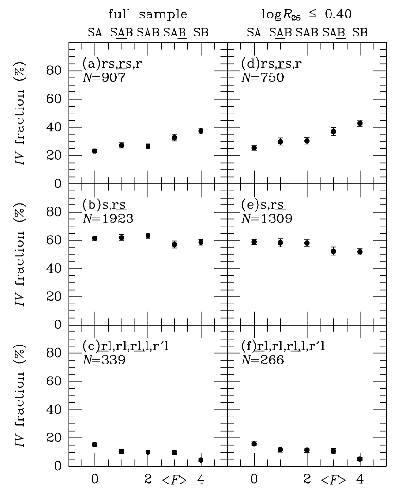
Figure 9: Distribution of CVRHS inner varieties versus family

Table 11: Statistics of Inner Varieties by family

$F$	$n$	rs,$\underline{\rm r}$s,r	s,r$\underline{\rm s}$	,rl,r$\underline{\rm l}$,l,r′l
		$f$%	$f$%	$f$%
1	2	3	4	5
	Full Sample	$N$=3169
0.0	1021	23.2$\pm$ 1.3	61.4$\pm$ 1.5	15.4$\pm$ 1.1
1.0	457	27.4$\pm$ 2.1	61.9$\pm$ 2.3	10.7$\pm$ 1.4
2.0	631	26.6$\pm$ 1.8	63.2$\pm$ 1.9	10.1$\pm$ 1.2
3.0	405	32.8$\pm$ 2.3	57.0$\pm$ 2.5	10.1$\pm$ 1.5
4.0	655	37.3$\pm$ 1.9	58.5$\pm$ 1.9	4.3$\pm$ 0.8
all $F$	3169	28.6$\pm$ 0.8	60.7$\pm$ 0.9	10.7$\pm$ 0.5
	$logR_{25}$ $\leq$ 0.40	$N$=2325
0.0	760	25.3$\pm$ 1.6	58.9$\pm$ 1.8	15.8$\pm$ 1.3
1.0	318	29.9$\pm$ 2.6	58.2$\pm$ 2.8	11.9$\pm$ 1.8
2.0	443	30.5$\pm$ 2.2	58.0$\pm$ 2.3	11.5$\pm$ 1.5
3.0	287	36.9$\pm$ 2.8	52.3$\pm$ 2.9	10.8$\pm$ 1.8
4.0	517	42.9$\pm$ 2.2	52.0$\pm$ 2.2	5.0$\pm$ 1.0
all $F$	2325	32.3$\pm$ 1.0	56.3$\pm$ 1.0	11.4$\pm$ 0.7

Table 12 summarizes the numbers of different kinds of outer features recognized in CVRHS classifications of EFIGI galaxies, including what Buta (2017b) refers to as “outer resonant subclasses": R₁, R${}_{1}^{\prime}$, R₁R${}_{2}^{\prime}$, and R${}_{2}^{\prime}$, of which 172 examples are included. Other types of outer features include outer lenses (L), outer rings (R), and outer ring lenses (RL) (see section 8.9), outer pseudorings (R^′) not clearly in any other subcategory, outer pseudoring-lenses (R^′L), and a variety of multiple outer feature categories such as a doubled outer ring (RR) and doubled outer pseudorings (R^′,R^′). Only 24% of the galaxies in the full EFIGI sample are recorded as having an outer feature in Table 4. Figure 10 shows the percentages of galaxies having an outer feature as a function of CVRHS stage. Like inner rings and pseudorings, outer features are most common near stage Sab and decrease in frequency towards earlier or later types, having the lowest frequency in Sc galaxies (see also de Lapparent et al. 2011). Surprisingly, the relative frequency of outer features has a secondary peak at stages later than Sc. Consistent with Comerón et al. (2014), outer features in the EFIGI sample are infrequent at stages later than Sb.

Table 13 highlights the mean stage associated with 10 outer feature types or groups of types having 10 or more galaxies. Outer lenses (L) are the main outer features characteristic of early-type disk galaxies (S0^o to S0⁺), while outer pseudorings are characteristic of much later types (S$\underline{\rm a}$b to Scd). The outer resonant subclasses are found in the range S0/a to Sa$\underline{\rm b}$, with R${}_{1}^{\prime}$ cases averaging about half a stage earlier than R${}_{2}^{\prime}$ cases. This range is similar to that found by de Lapparent et al. (2011). Outer ring-lenses (RL) average at stage S0/a (S0^- to Sb), while outer rings (R) average at stage Sa (S0^o to S$\underline{\rm b}$c). Table 13 also summarizes the mean family classification for each outer feature type. The weakest bars are found for outer rings, lenses, ring-lenses, and pseudorings, while the strongest bars are found for the outer resonant subclasses, especially for type R${}_{1}^{\prime}$.

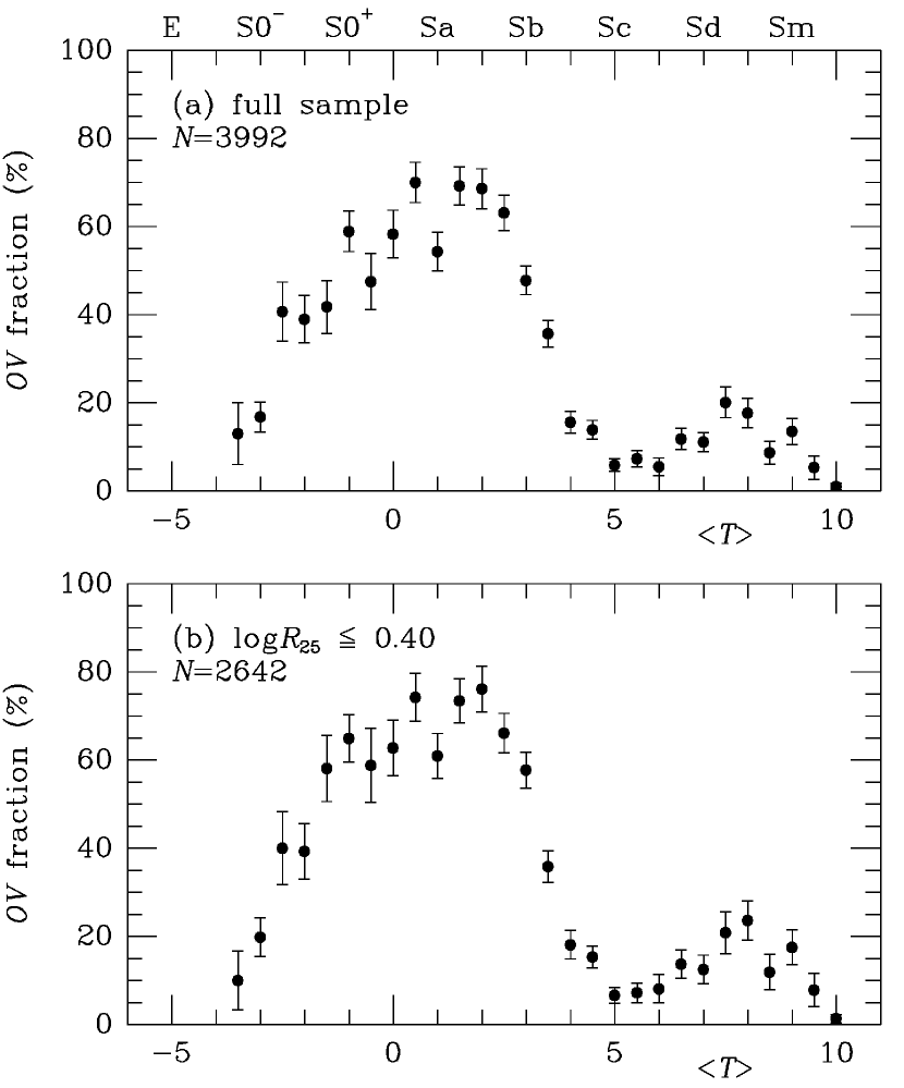
Figure 10: Outer variety fraction as a function of CVRHS stage

The distribution of arm classes, as defined by Elmegreen and Elmegreen (1987), is shown in Figure 11 and Table 15. AC 1–4 include mainly flocculent spirals, while AC 5–12 include mainly grand design spirals. The sample includes 21–22% of the flocculent types and 78–79% of the grand design types. Of the latter, most are grand design multi-armed spirals which account for 29% of the full sample and 33% of the restricted sample. Figure 12 shows the mean stage as a function of arm class. The flocculent categories average between stages S$\underline{\rm c}$d to Sdm, while the strongest grand design categories average between stages Sab and Sbc. This implies that AC1-4 galaxies are generally less luminous than AC 8-12 galaxies, as shown by Figure 2 of de Lapparent et al. (2011).

An important issue that can be examined with the EFIGI sample is the relative populations of the different “cells" of the CVRHS classification volume. A cell generally consists of a combination of stage, family, and variety, examples being SB(s)cd and S$\underline{\rm A}$B(r$\underline{\rm s}$)b. For this analysis, additional features such as outer varieties, lenses, nuclear structures, ansae bars, X patterns, and extra inner varieties are ignored. This leaves 25 cells at each CVRHS stage. The relative populations of these cells for the EFIGI sample are shown in Figures 13- 15 for three CVRHS stage intervals: S$\underline{\rm 0}$/a to Sa$\underline{\rm b}$ (early subgroup), Sb to S$\underline{\rm c}$d (intermediate subgroup), and Scd to Sm (late subgroup). From these it is clear that the cells of the CVRHS system are not uniformly populated. There are distinct nonuniformities: the intermediate subgroup emphasizes cell SA(s) while the late subgroup emphasizes cell SB(s). Only for the early subgroup are the populations of the cells relatively uniform.

The histograms in Figure 16 show these trends another way by plotting the number of galaxies in the 16 outer cells of each stage subgroup going counter-clockwise from cell SAB(r). These show that the diversity of spiral galaxy morphology diminishes with advancing stage. The original de Vaucouleurs (1959) classification volume tried to show this by narrowing down the volume from stage S0/a to stage Im.

Table 12: Statistics of Outer Features

Feature	$n$	Feature	$n$	Feature	$n$
1	2	1	2	1	2
(L)	116	(R${}_{1}^{\prime}$)	95	(R′,R)	7
(L:)	1	(R${}_{1}^{\prime}$L)	4	(R′,R1R${}_{2}^{\prime}$)	1
(L,R)	1	(R${}_{1}^{\prime}$R${}_{2}^{\prime}$)	4	(R′,RL)	1
(L,RL)	1	(R1R2)	1	(R′,R′)	13
(L,R′)	3	(R1R${}_{2}^{\prime}$)	19	(R′:,R${}_{2}^{\prime}$)	1
(PR)	1	(R${}_{2}^{\prime}$)	37	(R′L)	73
(R)	65	(RL)	58	(R′L,RL)	1
(R:)	4	(RL,L)	1	(R′L,R′)	1
(R?)	1	(RL,R)	1	(R′L,R′L)	1
(R,R′)	2	(RL,R′)	1	(RR)	2
(R1)	9	(RL?)	1	(R$\underline{\rm{L}}$)	4
(R${}_{12}^{\prime}$)	1	(R′)	551	(Rdust)	1
(R1L)	2	(R′,L)	1	no outer feature	3371

Table 13: Mean stages and families for outer features of different types

Feature	$<T>$	$\sigma_{1}$	$n$
1	2	3	4
(L)	-1.3	1.9	115
(R1), (R1L)	-0.2	1.2	11
(RL)	0.0	2.8	58
(R)	0.7	2.8	65
(R1R${}_{2}^{\prime}$),(R${}_{1}^{\prime}$R${}_{2}^{\prime}$),(R1R2)	1.5	1.3	24
(R${}_{1}^{\prime}$)	2.0	1.1	95
(R′L)	2.0	2.3	73
(R${}_{2}^{\prime}$)	2.6	1.5	37
(R′,R′)	3.0	1.4	13
(R′)	3.7	2.4	550
Feature	$<F>$	$\sigma_{1}$	$n$
1	2	3	4
(R′L)	1.3	1.4	73
(R′,R′)	1.5	1.5	13
(RL)	1.7	1.5	55
(R′)	1.8	1.5	547
(R)	1.8	1.4	65
(L)	1.9	1.7	115
(R${}_{2}^{\prime}$)	2.2	1.0	37
(R1R${}_{2}^{\prime}$),(R${}_{1}^{\prime}$R${}_{2}^{\prime}$),(R1R2)	2.6	1.3	24
(R1), (R1L)	2.6	1.2	11
(R${}_{1}^{\prime}$)	3.0	0.9	95

Table 14: Outer Variety fraction versus stage

$T$	$f_{bar}$(%)	$N(T)$	$T$	$f_{bar}$(%)	$N(T)$
1	2	3	1	2	3
	Full Sample	$N$=3992
-3.5	13.0$\pm$7.0	23	4.0	15.6$\pm$ 2.5	211
-3.0	16.8$\pm$3.4	119	4.5	13.9$\pm$ 2.1	280
-2.5	40.7$\pm$6.7	54	5.0	5.9$\pm$ 1.4	289
-2.0	39.0$\pm$5.4	82	5.5	7.3$\pm$ 1.8	205
-1.5	41.8$\pm$6.0	67	6.0	5.5$\pm$ 2.0	128
-1.0	58.9$\pm$4.6	112	6.5	11.8$\pm$ 2.4	178
-0.5	47.5$\pm$6.4	61	7.0	11.1$\pm$ 2.2	207
0.0	58.3$\pm$5.4	84	7.5	20.1$\pm$ 3.5	134
0.5	70.0$\pm$4.6	100	8.0	17.7$\pm$ 3.3	130
1.0	54.3$\pm$4.4	129	8.5	8.7$\pm$ 2.6	115
1.5	69.2$\pm$4.3	117	9.0	13.5$\pm$ 3.0	133
2.0	67.9$\pm$4.5	106	9.5	5.3$\pm$ 2.6	76
2.5	63.1$\pm$4.0	149	10.0	1.0$\pm$ 0.7	203
3.0	48.0$\pm$3.2	248	all $T$	27.2$\pm$ 0.7	3992
3.5	35.7$\pm$3.0	252	….	…………..	….
	$logR_{25}$ $\leq$ 0.40	$N$=2642
-3.5	10.0$\pm$6.7	20	4.0	18.1$\pm$ 3.2	144
-3.0	19.8$\pm$4.4	81	4.5	15.3$\pm$ 2.5	209
-2.5	40.0$\pm$8.3	35	5.0	6.6$\pm$ 1.8	183
-2.0	39.3$\pm$6.3	61	5.5	7.2$\pm$ 2.2	139
-1.5	58.1$\pm$7.5	43	6.0	8.1$\pm$ 3.2	74
-1.0	64.9$\pm$5.4	77	6.5	13.7$\pm$ 3.2	117
-0.5	58.8$\pm$8.4	34	7.0	12.5$\pm$ 3.2	104
0.0	62.7$\pm$6.3	59	7.5	20.8$\pm$ 4.8	72
0.5	74.2$\pm$5.4	66	8.0	23.6$\pm$ 4.5	89
1.0	60.9$\pm$5.1	92	8.5	11.9$\pm$ 4.0	67
1.5	73.4$\pm$5.0	79	9.0	17.5$\pm$ 3.9	97
2.0	76.1$\pm$5.2	67	9.5	7.8$\pm$ 3.8	51
2.5	66.1$\pm$4.5	109	10.0	1.3$\pm$ 0.9	158
3.0	57.7$\pm$4.1	142	all $T$	30.3$\pm$ 0.9	2642
3.5	35.8$\pm$3.6	173	….	……………	….

Figure 11: Distribution of Elmegreen Arm Classes

Table 15: Statistics of Arm Classes

Arm Class	$n$	%$N$	$<T>$	$\sigma_{1}$
1	2	3	4	5
		full sample ($N$=2417)
AC 1	110	4.6$\pm$0.4	7.9	1.5
AC 2	109	4.5$\pm$0.4	6.6	1.7
AC 3	102	4.2$\pm$0.4	5.5	1.7
AC 4	215	8.9$\pm$0.6	7.5	1.8
AC 5	201	8.3$\pm$0.6	5.5	1.5
AC 6	151	6.2$\pm$0.5	4.7	1.6
AC 7	102	4.2$\pm$0.4	5.0	1.5
AC 8	459	19.0$\pm$0.8	2.3	1.7
AC 9	693	28.7$\pm$0.9	4.4	1.1
AC 12	275	11.4$\pm$0.6	3.9	1.5
		$logR_{25}$ $\leq$ 0.40 ($N$=1806)
AC 1	83	4.6$\pm$0.5	8.0	1.5
AC 2	77	4.3$\pm$0.5	6.8	1.7
AC 3	59	3.3$\pm$0.4	5.6	1.7
AC 4	153	8.5$\pm$0.7	7.6	1.7
AC 5	150	8.3$\pm$0.6	5.7	1.4
AC 6	99	5.5$\pm$0.5	4.8	1.6
AC 7	41	2.3$\pm$0.4	4.8	1.5
AC 8	343	19.0$\pm$0.9	2.2	1.7
AC 9	604	33.4$\pm$1.1	4.4	1.1
AC 12	197	10.9$\pm$0.7	3.7	1.6

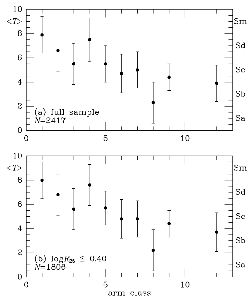
Figure 12: Mean stages of Elmegreen Arm Classes

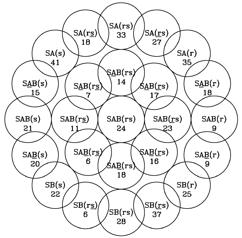
Figure 13: Distribution of EFIGI galaxies in cells of the CVRHS system from stages S$\underline{\rm 0}$/a to Sa$\underline{\rm b}$.

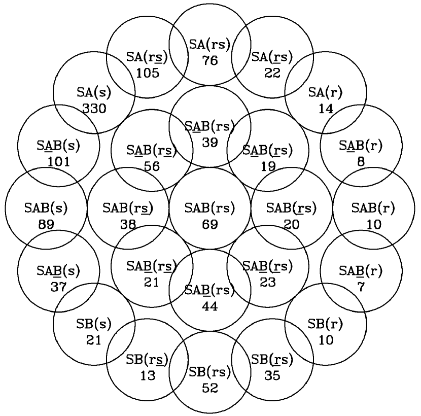
Figure 14: Distribution of EFIGI galaxies in cells of the CVRHS system from stages Sb to S$\underline{\rm c}$d.

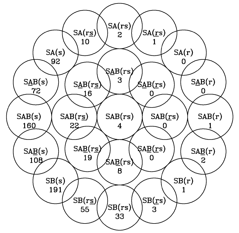
Figure 15: Distribution of EFIGI galaxies in cells of the CVRHS system from stages Scd to Sm.

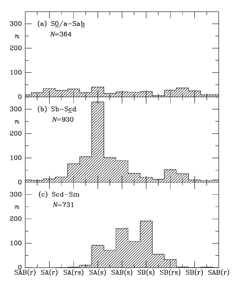
Figure 16: Histograms of the number of EFIGI galaxies within the 16 outer cross-sectional cells of the CVRHS.

Table 16 provides an inventory of other features recognized in the EFIGI galaxies. A barlens (bl) is a recently recognized feature (Laurikainen et al. 2011) that is intermediate in scale between a nuclear lens (nl) and an inner lens (l), relative to the bar length. Generally, in galaxy morphology, a lens is a feature with a shallow brightness gradient interior to a sharper edge (section 8.9). Barlenses are most obvious in strong bar cases, and have been closely linked to “boxy/peanut" bulges (Laurikainen and Salo 2017; Salo and Laurikainen 2017). Table 4 includes 272 recognized cases of a barlens, or 6.1% of the full EFIGI sample. The average stage of barlens galaxies in Table 4 is S$\underline{\rm a}$b, and they are found mainly in the stage range S$\underline{\rm 0}$/a to S$\underline{\rm b}$c.

Nuclear rings (nr) and related features, such as nuclear pseudorings (nr^′), nuclear ring-lenses (nrl), and nuclear lenses (nl) are recognized in only 102 of the sample galaxies. These occur at an average stage of Sa$\underline{\rm b}$ over the stage range S0/a to Sb$\underline{\rm c}$. While the mean family of barlens galaxies is SA$\underline{\rm B}$, that for nuclear rings in the sample is S$\underline{\rm A}$B. This subtle distinction may be a selection effect. Comerón et al. (2010) showed that nuclear rings tend to be smaller in more strongly-barred galaxies, making them less likely to be recognized. Nuclear bars (nb) and nuclear spirals (ns) tend to be phenomena of later stages, on average: Sb for nuclear bars and S$\underline{\rm b}$c for nuclear spirals. Resolution effects in detecting nuclear features are discussed by Buta (2017a).

Table 16 also includes the mean stages, families, and ranges for X patterns and ansae-type bars. A galaxy classified as SB_x (or SAB_x) may either be a case of an edge-on boxy peanut bulge or a lower inclination galaxy having a strong bar with an inner boxy character (section 8.3). A galaxy where the bar has a bright, rounder inner section flanked by two enhancements (“ansae") is called an ansae-type bar (deVA; Sandage 1961), and is classified as type SB_a (or SAB_a). Some galaxies show both ansae and an inner boxiness; these are classified as SB_xa or SB_ax. In Table 4, B_x and B_a galaxies both average being found in S$\underline{\rm a}$b galaxies, while the B_xa and B_ax cases average at stage S0/$\underline{\rm a}$.

Spindle (or highly-inclined) galaxies (sp) constitute 23% of the full EFIGI sample. An additional 258 (5.8%) of the sample are classified as warped spindles (spw). Spindles and warped spindles average near stage Sc.

Finally, the classifications of 665 EFIGI galaxies (14.9% of the sample) are appended with “pec", indicating a peculiar feature, often an asymmetry or peculiar dust pattern.

Table 16: Other Features

Feature	$<Stage>$	Range	$<Family>$	Range	$n$	%$N$=4458
1	2	3	4	5	6	7
bl	S$\underline{\rm a}$b	S$\underline{\rm 0}$/a to S$\underline{\rm b}$c	SA$\underline{\rm B}$	SA$\underline{\rm B}$ to SB	272	6.1
nr,nr′,nrl,nl	Sa$\underline{\rm b}$	S0/a to Sb$\underline{\rm c}$	S$\underline{\rm A}$B	SA to SA$\underline{\rm B}$	102	2.3
nb	Sb	Sa to S$\underline{\rm c}$d	SAB	S$\underline{\rm A}$B to SA$\underline{\rm B}$	43	1.0
ns	S$\underline{\rm b}$c	Sa to Scd	SA$\underline{\rm B}$	SAB to SB	13	0.3
Bx	S$\underline{\rm a}$b	S$\underline{\rm 0}$/a to Sbc	SAB	S$\underline{\rm A}$B to SB	92	2.1
Ba	S$\underline{\rm a}$b	S0+ to Sbc	SA$\underline{\rm B}$	SAB to SB	218	4.9
Bxa,Bax	S0/$\underline{\rm a}$	S0+ to Sab	SA$\underline{\rm B}$	SAB to SB	44	1.0
sp	Sb$\underline{\rm c}$	Sa to Sdm	…..	…..	1032	23.1
spw	Sc	Sa$\underline{\rm b}$ to S$\underline{\rm d}$m	…..	…..	258	5.8
pec	Sb	S0+ to Sd	…..	…..	665	14.9

8 Morphological Highlights of the Catalogue

In this section, attention is brought to exceptional or special morphological features found in the EFIGI sample. These have not necessarily been previously studied in spite of multiple classifiers.

8.1 Extremely Oval Inner Rings in SB Galaxies

The typical inner ring in an SB galaxy has an intrinsic axis ratio of 0.81$\pm$0.06 (Buta 1995). An extremely oval inner ring is one which has a much smaller intrinsic axis ratio than this. In the EFIGI database, NGC 4334 (Figure 17, upper right) is an interesting example where the intrinsic axis ratio of the inner ring is $\approx$0.5. Such extremely oval inner rings are rare but are important for what they highlight about barred galaxy dynamics and star formation. The distribution of star formation around inner rings is very sensitive to ring shape (Crocker et al. 1996; Grouchy et al. 2010). Figure 17 shows the wide range of intrinsic shapes of inner rings that any theory would have to explain, based on two examples from Table 4 and four examples from the Catalogue of Southern Ringed Galaxies (CSRG; Buta 1995). Other examples are illustrated by Buta (2017a).

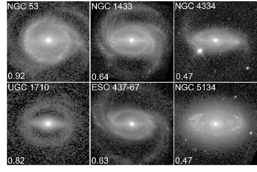
Figure 17: Montage showing the wide range of intrinsic shapes of inner rings in SB galaxies, based on deprojected $B$ or $g$-band images (foreground stars removed in some panels). Only NGC 4334 and UGC 1710 are in the EFIGI sample; the remainder are from the CSRG. The ring face-on axis ratio is given at lower left.

8.2 Young and old stellar population bar ansae

A large sample of color images as provided by the SDSS allows us to see certain phenomena in a different light. One such phenomenon is bar ansae, which we mentioned in section 7. These features are common among early-type barred galaxes (Martinez-Valpuesta et al. 2007), and even inspired an early theoretical study (Danby 1965). In the discussion by Martinez-Valpuesta et al. (2007), it was noted that most ansae appear stellar dynamical in nature, although at least one example of star-forming ansae (in NGC 4151) was presented. Ansae have recently been shown using numerical simulations to form in the disk-shaped remnant of the merger of two spiral galaxies (Athanassoula et al. 2016).

EFIGI provides many examples that can change our view of these features. Figure 18 shows two contrasting cases: NGC 5375, an S$\underline{\rm b}$c-type spiral with old stellar population ansae, and UGC 9732, an Sb$\underline{\rm c}$-type spiral with strong blue ansae. Old stellar-population ansae are of three types: linear, short arcs, and circular spots, and are generally seen in early-to-intermediate type spirals. In contrast, blue ansae seem to avoid early-type galaxies. Linear ansae can account for the strong boxy shapes of the ends of some bars (Athanassoula et al. 1990). Blue ansae could be linked to extremely oval inner rings.

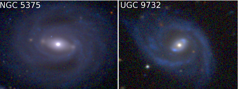
Figure 18: Two intermediate-type spirals showing contrasting bar ansae colors.

8.3 X galaxies and Box/Peanut Bulges

X patterns in galaxies were first recognized by Whitmore & Bell (1988), who suggested the strange features are caused by accretion of a companion. However, as reviewed by Athanassoula (2005), box/peanut bulges are nothing more than side-on views of bars. X patterns may be an optical illusion and are believed to show the vertical resonant structure of bars (Bureau & Freeman 1999; Athanassoula & Bureau 1999; Bureau et al. 2004, 2006).

The EFIGI database includes many excellent examples of X patterns and box/peanut bulges. Four conventional edge-on examples are shown in Figure 19. In non-edge-on early-type galaxies, an X pattern is often seen in an inner boxy zone that is generally flanked by ansae. In Figure 19, NGC 4215 has two very strong ansae flanking a very diffuse box/peanut zone. This case, more than any other, suggests that ansae are much flatter than the inner zones of ansae bars.

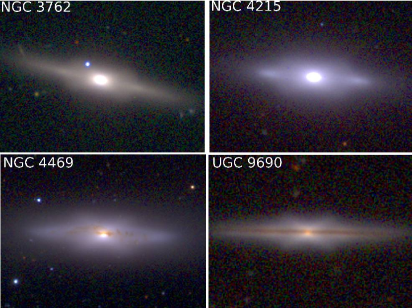
Figure 19: Four almost exactly edge-on EFIGI S0 and S galaxies showing strong X and box/peanut bulge patterns

8.4 Hexagonal Zone X Galaxies

NGC 7020 (Figure 20,upper left) is an unusual non-EFIGI early-type southern galaxy with an exceptionally bright and well-defined outer ring surrounding a distinct inner hexagonal zone that appears crossed by a subtle X pattern (Buta 1990). It is the prototype of what may be called a “hexagonal zone X galaxy." While X patterns are most commonly seen in nearly edge-on galaxies and are thought to be related to bars, NGC 7020 is inclined only 69^o (deVA). The EFIGI sample includes at least 15 cases that resemble NGC 7020 in various ways.

Hexagonal zone X galaxies are easily explained in terms of an inclined view of a bar having a 3D inner section flanked by two flat, almost linear ansae. The X arises from vertical resonant bar orbits (e.g., Athanassoula 2005). Figure 20 shows how the hexagonal zones come about: a galaxy having two linear bar ansae is viewed at an intermediate angle that allows one set of the ends of the X to project as connecting to one pair of ends of the ansae. This effect is especially well seen in EFIGI galaxy NGC 2878 (Figure 20, upper right), in which the hexagonal zone X morphology is the main morphological feature. The projection of one arm of the X against the ends of the ansae gives the likely false impression that NGC 2878 is a spiral galaxy.

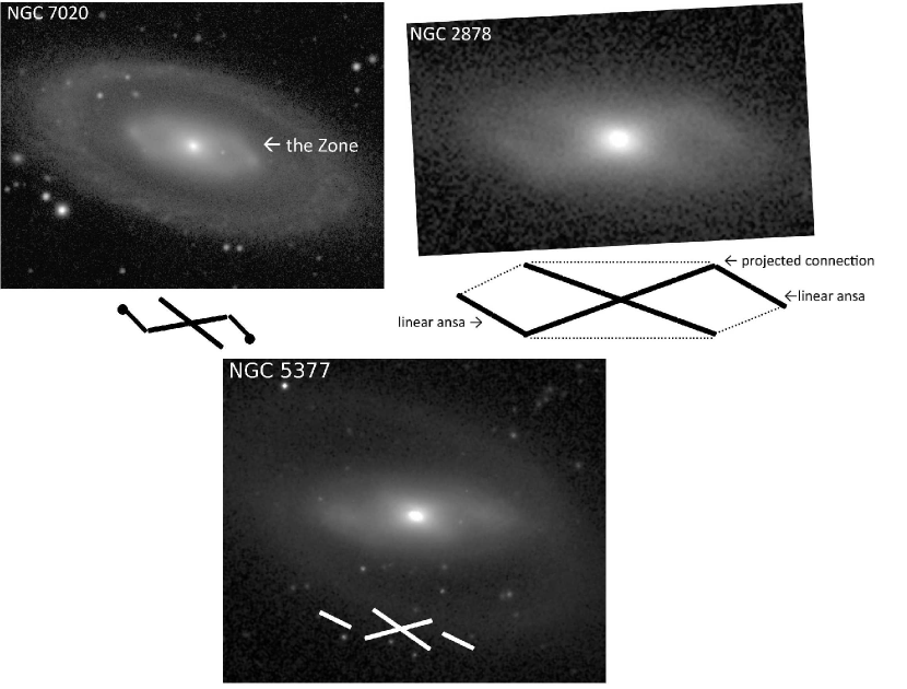
Figure 20: top left: $B$-band image of NGC 7020, a southern galaxy showing a bright outer ring surrounding an unusual hexgonal zone crossed by a subtle X pattern (Buta 1990). top right: EFIGI galaxy NGC 2878 also shows a hexagonal zone X pattern; however, in this case the pattern represents the whole galaxy, not just the inner section; bottom: EFIGI galaxy NGC 5377, showing an inner pattern similar to NGC 7020 but lacking the hexagonal shape. The schematics below each image show how the likely projection of a 3D X-pattern associated with the inner part of a bar projects onto what are likely flat, linear ansae.

The bottom panel of Figure 20 shows NGC 5377, an inclined (but not edge-on) early-type EFIGI spiral showing a prominent inner X pattern and bright, slightly curved ansae (Laurikainen et al. 2011). Although the inner zone is similar to NGC 7020, the appearance is not hexagonal. In this case, as shown by the schematic, the arms of the X do not project onto the ends of the ansae. The appearance of the inner zone is that of a strongly skewed spiral bar. In this case, however, the skewness is mostly an artifact of projection effects. This is consistent with the numerical simulations of Athanassoula et al. (2015) and most recently with simulations made by Erwin and Debattista (2013) and Salo and Laurikainen (2017).

8.5 Skewed Spiral Bars

Erwin and Debattista (2013) show that the combination of a 3D box/peanut bulge with much flatter bar ends can cause the bar of a galaxy to take on a “box + spurs" look. Such bars can look skewed in characteristic ways. In these bars, the observed skewness is not necessarily real, but a projection effect between the 2D and 3D parts of the bar. However, when spiral-like bars are seen in relatively face-on galaxies, the skewness is likely to be real.

One of the best cases in the EFIGI sample is IC 671 (Figure 21). The galaxy shows a spiral-like bar within a large inner pseudoring. Outer isophotes favor an inclination of only 37^o. Fourier analysis of a deprojected image gives a gaussian relative $m$=2 intensity profile for the bar (Buta et al. 2006), but the phase, $\phi_{2}$, for this bar is not constant with radius (Figure 21, right).

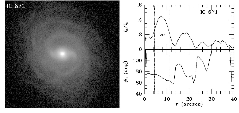
Figure 21: The bar in IC 671 is skewed in a trailing sense. The graphs show the $m$ = 2 relative Fourier amplitudes and phases as a function of radius. The vertical dotted lines delineate the bar region of the galaxy.

Figure 22 shows two even more low inclination systems showing skewed bars. UGC 1794 is a clear and unambiguous example of a “spiral bar" (Buta 1986), a spiral distributed within a broad but very bar-like oval zone. The ($\phi_{2}$,ln$r$) profile (Figure 23, left) for UGC 1794 shows two radial zones where $\phi_{2}$ versus ln$r$ is linear. For the bar-spiral zone, the pitch angle is 61^o, while for the outer arms the pitch angle is 34^o. For NGC 4719, the skewed bar is in the radial zone indicated in Figure 23, right. From a linear fit to this zone, the pitch angle of the bar-spiral is 80^o. The outer arms of this galaxy are partly distorted towards an R${}_{1}^{\prime}$ outer pseudoring, and as a result the pitch angle tends to 0^o in the outer disk.

Bar skewness, if real, can drive secular evolution of the stellar mass distribution through the potential-density phase shift that would result from the skewed shape (Zhang 1996; Zhang & Buta 2007).

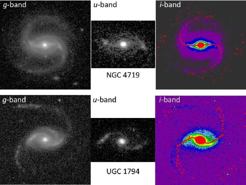
Figure 22: Bar skewness in the nearly face-on galaxies UGC 1794 and NGC 4719. The skewness is mapped in the right frames using the phase of the $m$=2 Fourier component. The $u$-band images in both cases show an ansae character in the distribution of star formation. The estimated inclination of NGC 4719 is 22^o based on ellipse fits to $g$-band outer isophotes. UGC 1794 has been assumed to be face-on.

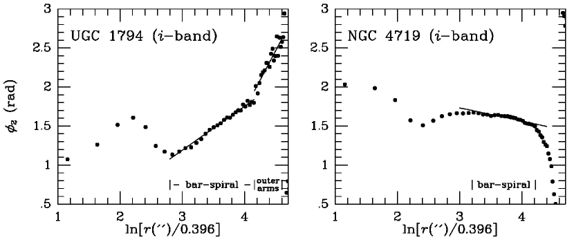
Figure 23: Graphs of phase $\phi_{2}$ versus the natural log of the radius for UGC 1794 and NGC 4719, useful to estimate the pitch angles of the bar-spirals. left: The profile for UGC 1794 shows two radial zones where $\phi_{2}$ versus ln$r$ is linear. For the bar-spiral zone, the pitch angle is 61^o, while for the outer arms the pitch angle is 34^o. right: For NGC 4719, the skewed bar is in the radial zone indicated. From a linear fit to this zone, the pitch angle of the bar-spiral is 80^o. The outer arms of this galaxy are partly distorted towards an R${}_{1}^{\prime}$ outer pseudoring, and as a result the pitch angle tends to 0^o in the outer disk.

8.6 Intrinsic Bar-Ring Misalignment

Statistics of the projected relative position angle between the long axis of a bar and the major axis of a ring have indicated that rings are intrinsically elongated and have preferred alignments with respect to bars (Buta 1995). The “rule" for inner SB rings is alignment parallel to the bar, while the “rule" for R₁ and R${}_{1}^{\prime}$ outer rings is alignment perpendicular to the bar. In spite of what statistics showed, however, Buta (1995) nevertheless identified several nearby face-on galaxies where an inner ring and a bar are significantly misaligned, clear counter-examples to the normal situation. More recently, Comerón et al. (2014) used statistics of rings in the S⁴G (Sheth et al. 2010) to show that, among late-type galaxies, there is a significant population of inner rings that are misaligned and even perpendicular to the bars they enclose.

The EFIGI sample has brought attention to bar-outer pseudoring misalignment. An excellent example (previously noted by Buta 2017b) is IC 2473, a galaxy showing a strong outer pseudoring having a clear dimpled, figure-eight shape (Figure 24). These are characteristics of outer resonant subclass outer pseudorings symbolized in the CVRHS by R${}_{1}^{\prime}$, a type generally aligned perpendicular to bars (Buta 1995). Yet, when deprojected, Figure 24 shows that the R${}_{1}^{\prime}$ ring in IC 2473 is at an intermediate angle with the bar. It appears that in IC 2473, the inner (r) and outer (R${}_{1}^{\prime}$) are elongated nearly perpendicularly, and that the bar is misaligned with both features. Figure 24 compares IC 2473 with a deprojected $B$-band image of non-EFIGI galaxy ESO 437$-$67 (Buta & Crocker 1991), a more typical example where the same kinds of features have the standard alignments.

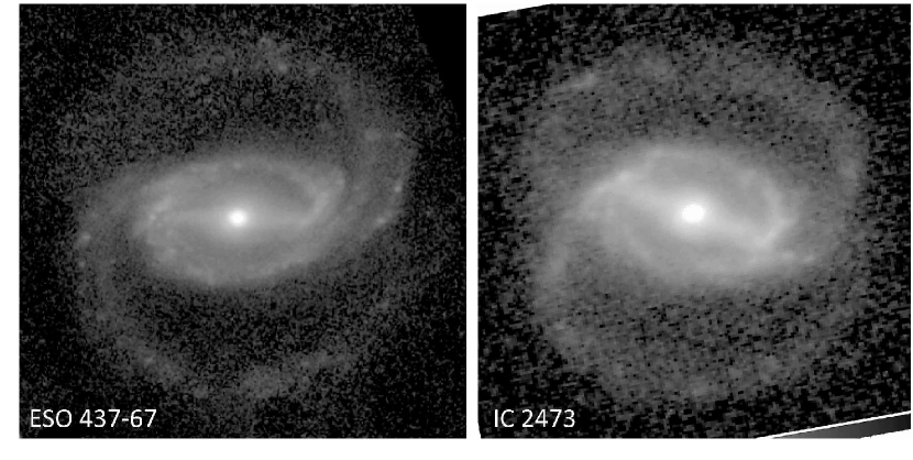
Figure 24: Deprojected images showing misaligned bar-R${}_{1}^{\prime}$ galaxy IC 2473 ($g$-band) with a more normal, aligned example ESO 437$-$67 ($B$-band; Buta & Crocker 1991)

Bar-ring misalignment is important because it challenges existing models of resonance rings and is unlikely to be a stable, long-term phenomenon. Such misalignment could point to the possibility that the bar has a different pattern speed from that of the combined rR${}_{1}^{\prime}$ pattern (e.g., Rautiainen & Salo 2000).

8.7 Barred spirals with non-outer pseudoring arms

Spiral patterns in nonbarred galaxies are usually logarithmic and can be described by a single value of the pitch angle. The spiral structure of barred galaxies can also be logarithmic, but shows more diversity through the existence of the outer resonant subclasses of outer rings and pseudorings. In these cases, the pitch angle of spiral arms is not constant with radius and the patterns close in characteristic ways, one of which is shown in Figure 25. The existence of such dynamically identifiable patterns has been attributed to secular evolution of more open spiral patterns and the role of pattern speeds on galaxy morphology (Buta & Combes 1996). While outer resonant subclass rings might be bar-driven patterns having the same pattern speed as the bar, it is likely that a logarithmic spiral in a barred galaxy has a pattern speed different from the bar and may be an independent pattern, not driven by the bar.

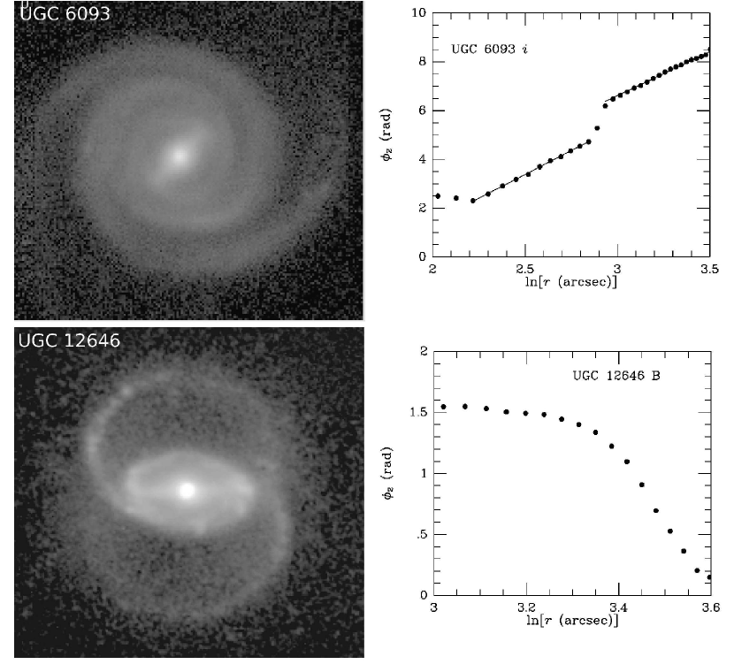
Figure 25: Comparison of two barred galaxies, one having logarithmic spiral structure (UGC 6093, assumed face-on) and the other non-logarithmic arms (UGC 12646, non-EFIGI sample, deprojected). The graphs show the Fourier $m$=2 phases of the arm patterns

8.8 Extreme Late-type Barred Spirals

In Table 4, SB(s)c$\underline{\rm d}$ is a common morphology involving extreme late-type galaxies with conspicuous bars. What makes these galaxies important is threefold: (1) they are essentially pure disk galaxies, a type that has been difficult to produce in cold dark matter simulations like the $\Lambda$CDM model (e.g., Mayer et al. 2008; see also Robertson et al. 2004); (2) the bars of these galaxies are very different from the typical bar seen in earlier types in that they lack a broad inner component, are probably vertically very thin and azimuthally relatively narrow, and are dominated by a younger stellar population; and (3) these galaxies are part of the tendency for the bar fraction to rise among late-type galaxies (e.g., Barazza et al. 2008).

Figure 26 shows 15 EFIGI sample galaxies classified as (or close to) type SB(s)c$\underline{\rm d}$ in Table 4. Apart from a somewhat irregular appearance, such galaxies look remarkably homogeneous with respect to bar and disk colors. More detailed study of such galaxies could shed important light on the nature of bars in a pure disk habitat.

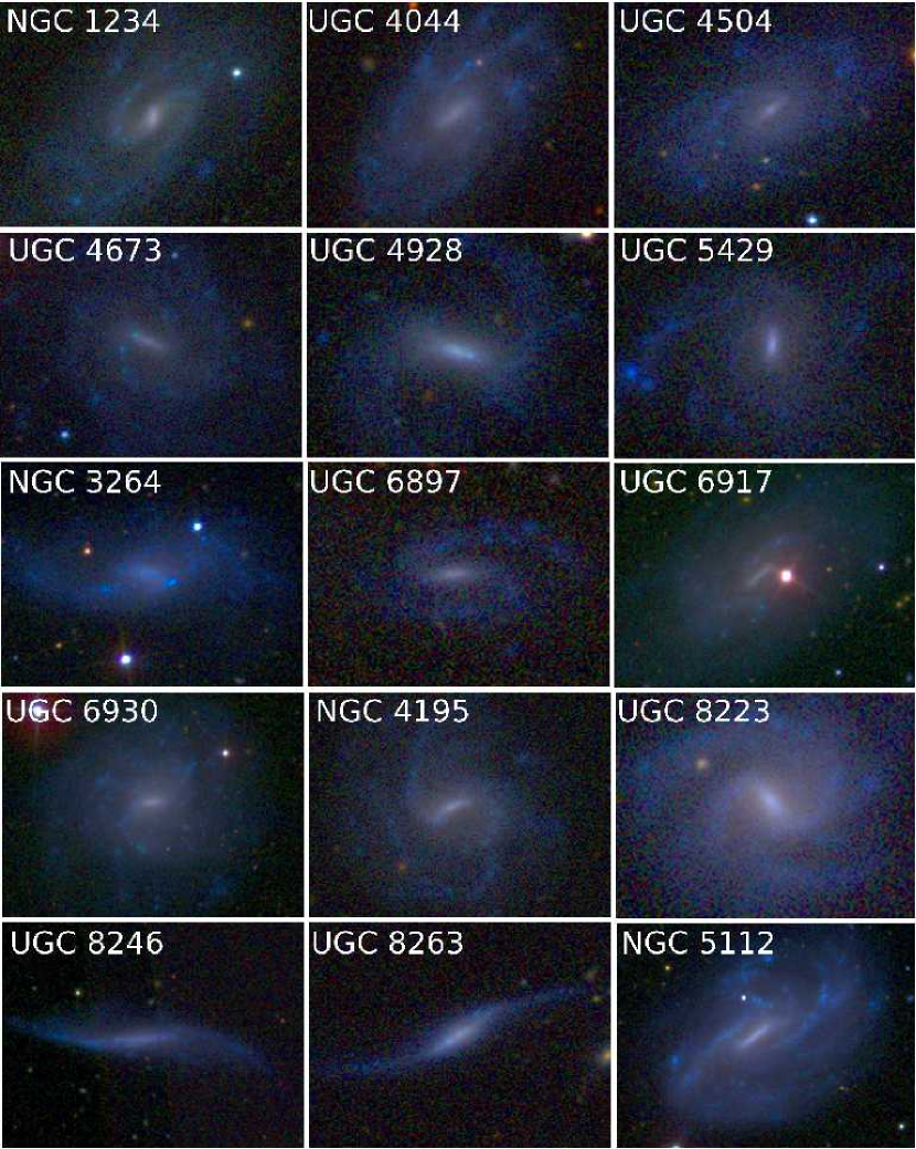
Figure 26: Fifteen EFIGI sample galaxies classified as (or close to) type SB(s)c$\underline{\rm d}$ in Table 4.

8.9 Ringed versus lensed galaxies

Rings and lenses in nonbarred galaxies are of special interest because the formation of both types of features is thought to be related to bars. A ring can form by gas accumulation at resonances, under the continuous action of gravity torques from a bar (Buta & Combes 1996). The origin of lenses is under debate. Kormendy (1979) argued that an inner lens may form from dissolution of a bar, owing to an interaction between a bar and the other components in a galaxy (see also Bournaud & Combes 2002). Alternatively, a lens may form from dissolution of a “dead" ring no longer forming any new stars (e. g., NGC 7702; Buta 1991). In a recent numerical study, Eliche-Moral et al. (2018) show that major mergers can account for much of the inner structure of S0 galaxies, including rings, ovals, lenses, and inner discs.

Although most rings do appear to be related to bars, the number of nonbarred galaxies with these features is not negligible. In fact, some of the most spectacular examples of star-forming rings are found in mostly nonbarred galaxies [e.g., NGC 4736 (Schommer & Sullivan 1976; deVA) and NGC 1553 (Kormendy 1984); see also Crocker et al. 1996 and Grouchy et al. 2010]. The weak link between rings and bars is further examined by Díaz-García et al. (2019).

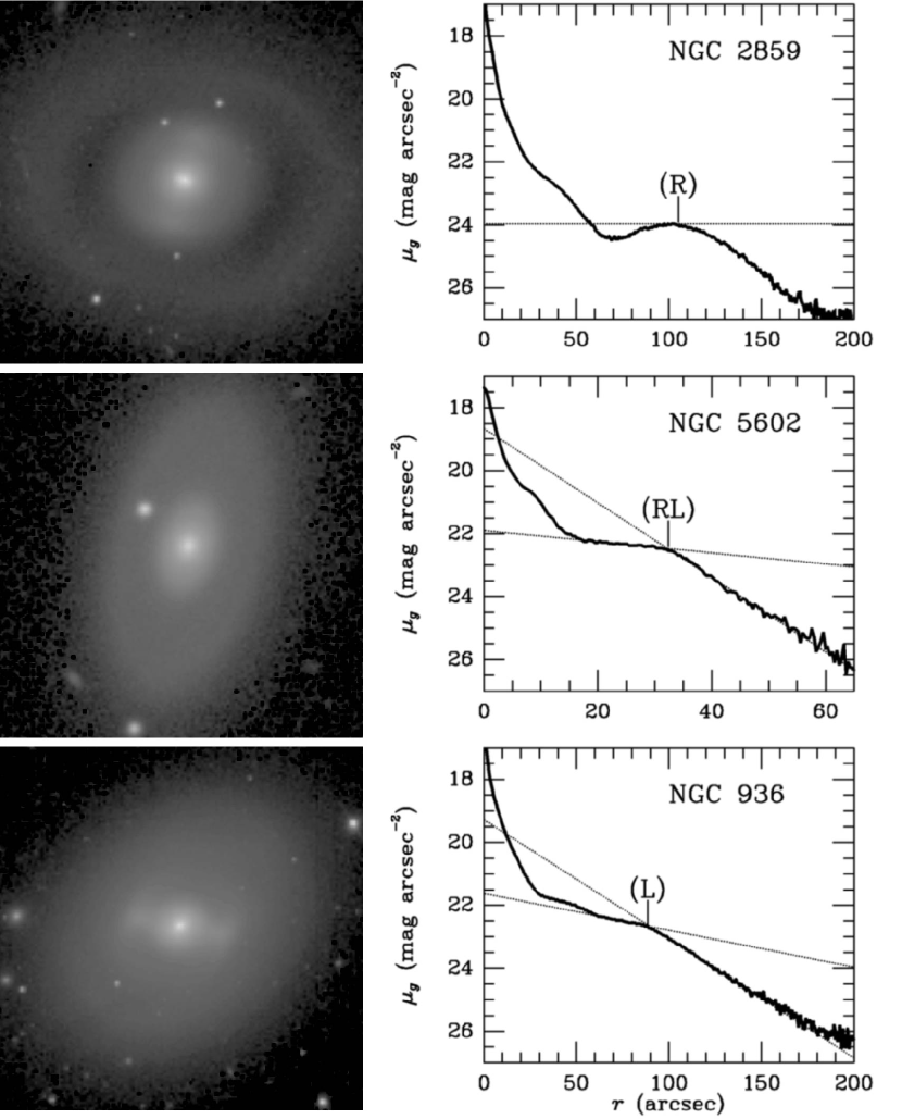
Figure 27: Mean major axis $g$-band luminosity profiles (right panels) of three EFIGI galaxies showing the distinction between outer rings (R), outer ring-lenses (RL), and outer lenses (L). The left panels show SDSS $g$-band images of the same galaxies in units of mag arcsec^-2. The lines for NGC 5602 and NGC 936 are fits to the inner and outer parts of the lens profiles.

The EFIGI sample includes some interesting examples of ringed and lensed galaxies. Figure 27 shows how the classifications (R), (RL), and (L) (outer ring, outer ring-lens, and outer lens, respectively) translate into mean major axis $g$-band surface brightness profiles for NGC 2859 (SA$\underline{\rm B}$), NGC 5602 (SA), and NGC 936 (SB). Although the outer feature of NGC 5602 is subtly ring-like in the SDSS $g$-band image, the major axis profile shows no clear enhancement, while the outer ring of NGC 2859 is a strong enhancement. The outer lens of NGC 936 is strongly sloped near its “edge" (intersection of the two lines).

NGC 3419 is a mostly SA galaxy which has a very bright inner lens (l) and a faint but distinct outer ring (Figure 28, left). The $g$-band mean surface brightness profile along the (l) major axis (Figure 28, right) provides a good example of the definition of a lens as a feature with a shallow brightness gradient interior to a sharp edge (Kormendy 1979).

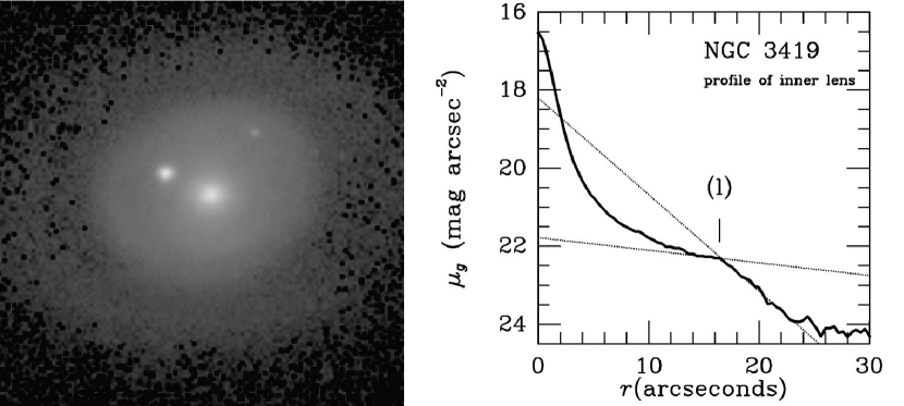
Figure 28: SDSS $g$-band image in units of mag arcsec^-2 (left) and mean major axis $g$-band luminosity profile (right) of NGC 3419, a strong inner lens galaxy. The lines are fits to the inner and outer parts of the lens profile.

9 The CVRHS system and Large-Scale Automated Galaxy Classification

Although the CVRHS system is a fairly accessible approach to galaxy classification, it may not be practical for it to be “crowd-sourced" in the manner of the Galaxy Zoo project, nor is it likely that the system will ever be directly applied to more than a few tens of thousands of galaxies. Yet, as noted by Domínguez Sánchez et al. (2019), astronomy is entering a new era of large surveys (e.g., Euclid, LSST, WFIRST, etc.) that will require the most sophisticated tools of automated classification possible to handle the literally millions of galaxies that will need to be classified.

A general requirement for automatic classification is a fairly large training set, i.e., a set of images of galaxies whose classifications are already known, either by expert classification or by the crowd-sourcing approach of Galaxy Zoo 2, for example. Domínguez Sánchez et al. (2018) use the detailed classifications of Nair and Abraham (2010) and Galaxy Zoo 2 to train a deep machine learning algorithm based on convolutional neural networks (Dieleman et al. 2015) to automatically classify 670,000 galaxies. In principle, the classifications in Table 4 could be used as such a training set, especially with regard to the numerical T-types and F-types. However, the complexities of inner, outer, and nuclear varieties, as well as other aspects of CVRHS morphology, may challenge automatic recognition.

The advantage of CVRHS morphology lies not only in its usefulness for training an automated classification algorithm, but also in recognizing peculiar or special cases of interest. This is true of all visual surveys, including Galaxy Zoo 2.

10 Summary

The EFIGI galaxy sample (Baillard et al. 2011) has been re-examined from the point of view of CVRHS classification. The main results from this study are:

1. a consistent set of detailed classifications of RC3 galaxies that likely represent an improvement on the many RC3 classifications that were based on small-scale sky survey prints. The CVRHS types have internal dispersions of $\sigma_{i}(T)$ = 0.7 stage intervals, $\sigma_{i}(F)$ = 0.6 family intervals, and $\sigma_{i}(IV)$ = 1.1 inner variety intervals.

2. good agreement between the mean stage and family classifications in Table 1 and those of Baillard et al. (2011), RC3, Nair & Abraham (2010), and Ann et al. (2015). The external dispersions in the CVRHS classifications are $\sigma_{e}(T)$ = 1.1 stage intervals and $\sigma_{e}(F)$ = 0.8 family intervals.

3. a bar fraction of 53%-67%, which is typical of a non-volume-limited sample like EFIGI. The peculiar feature of CVRHS bar classifications, which in the S⁴G mid-IR classifications of Buta et al. (2015) show a prominent minimum in bar fraction around stages Sbc to Sc, reappears in the classifications of the EFIGI galaxies. This is not necessarily a personal equation effect, but may show that the stage sequence for barred galaxies is not necessarily in step with that for nonbarred galaxies.

4. the highest relative frequency of inner rings and pseudorings, as well as the highest frequency of outer features, occurs near stage Sab. This is consistent with previous results and is one of the most important observations along the Hubble sequence.

5. the highest relative frequency of inner rings and pseudorings occurs in SB galaxies; however, the highest frquency of inner ring-lenses and lenses occurs in SA galaxies.

6. the sample emphasizes grand-design, multi-armed spirals in the type range Sab to Sbc; flocculent spirals in the sample average between S$\underline{\rm c}$d to Sdm.

7. the VRHS classification volume has a more asymmetric shape than usually depicted because of nonuniform fillings of the “cells" from earlier to later stages.

8. further verification of the wide range, $\approx$0.5-1.0, of the intrinsic face-on minor to major axis ratios of inner rings.

9. further recognition of the close relation between ansae bars and X patterns/box-peanut bulges.

10. recognition of bar-outer pseudoring misalignment among outer resonant subclass rings.

11. recognition of genuine bar skewness that in some galaxies could drive secular evolution.

12. identification of unusual barred galaxies having logarithmic outer spiral patterns rather than outer pseudorings

13. many new examples of bar ansae, particularly the previously under-appreciated class of blue ansae and the extension of ansae into later type galaxies.

14. an established connection between “hexagonal zone X galaxies" and projection effects in inclined bars with a 3D inner section.

15. finally, many excellent examples of different galaxy types as per the construction of the EFIGI sample by Baillard et al. (2011).

The author thanks the referee for helpful comments which improved this paper. This work was supported initially by a grant from the Research Grants Committee of the University of Alabama. Funding for the SDSS and SDSS-II has been provided by the Alfred P. Sloan Foundation, the Participating Institutions, the National Science Foundation, the U.S. Department of Energy, the National Aeronautics and Space Adiminstration, the Japanese Monbukagakusho, the Max Planck Society, and the Higher Education Funding Council for England. The SDSS website is http://www.sdss.org.

References

- (1) Adelman-McCarthy J., et al., 2006, ApJS, 162, 38
- (2) Ann H. B., Seo M., Ha D. K., 2015, ApJS, 217, 27 (ASH)
- (3) Athanassoula E., 2005, MNRAS, 358, 1477
- (4) Athanassoula E., Bureau M., 1999, ApJ, 522, 699
- (5) Athanassoula E., Rodionov S. A., Peschke N., Lambert J. C., 2016, ApJ, 821, 90
- (6) Athanassoula E., Morin S., Wozniak H., Puy D., Pierce M. J., Lombard J., Bosma A. 1990, MNRAS, 245, 130
- (7) Athanassoula E., Laurikainen E., Salo H., Bosma A., 2015, MNRAS, 454, 3843
- (8) Athanassoula E, Romero-Gómez M., Bosma A., Masdemont J. J., 2010, MNRAS, 407, 1433
- (9) Baillard A. et al., 2011, A&A, 532, 74
- (10) Barazza F. D., Jogee S., Marinova I., 2008, ASPC, 396, 351
- (11) Bournaud F., Combes F., 2002, A & A, 392, 83
- (12) Bureau M., Freeman, K. C., 1999, AJ, 118, 126
- (13) Bureau M., Athanassoula E., Chung A., Aronica, G., 2004, in Penetrating Bars Through Masks of Cosmic Dust, D. L. Block, et al., eds., Dordrecht, Springer, p. 139
- (14) Bureau, M., Aronica, G., Athanassoula, E., Dettmar, R.-J., Bosma, A., Freeman, K. C. 2006, MNRAS, 370, 753
- (15) Buta R., 1986, ApJS, 61, 609
- (16) Buta R., 1990, ApJ, 356, 87
- (17) Buta R., 1991, ApJ, 370, 130
- (18) Buta R., 1995, ApJS, 96, 39
- (19) Buta R., 2017a, MNRAS, 471, 4027
- (20) Buta R., 2017b, MNRAS, 470, 3819
- (21) Buta R., Combes F., 1996, Galactic Rings, Fund. of Cosmic Physics, 17, 95
- (22) Buta R., Crocker D. A., 1991, AJ, 102, 1715
- (23) Buta R. J., Corwin H. G., Odewahn, S. C., 2007, The de Vaucouleurs Atlas of Galaxies, Cambridge: Cambridge U. Press (deVA)
- (24) Buta R., Laurikainen E., Salo H., Block D.L., Knapen J.H., 2006, AJ, 132, 1859
- (25) Buta R., Mitra S., de Vaucouleurs G., Corwin H., 1994, AJ, 107, 118
- (26) Buta R. et al., 2015, ApJS, 217, 32
- (27) Comerón S., Knapen J. H., Beckman J. E., Laurikainen E., Salo H., Martí nez-Valpuesta I., Buta R. J., 2010, MNRAS, 402, 2462
- (28) Comerón S., et al., 2014, A & A, 562, 121
- (29) Crocker D. A., Baugus P.D., Buta R., 1996, ApJS, 105, 353
- (30) Danby J. M. A. 1965, AJ, 70, 501
- (31) de Lapparent V., Baillard A., Bertin E., 2011, A&A, 532, 74
- (32) de Vaucouleurs G., 1959, Handbuch der Physik, 53, 275
- (33) de Vaucouleurs G., 1963, ApJS, 8, 31
- (34) de Vaucouleurs G., de Vaucouleurs A., Corwin H. G., Buta R., Paturel G., & FouqueṔ., 1991, Third Reference Catalogue of Bright Galaxies, New York, Springer (RC3)
- (35) Díaz-García S., Díaz-Suárez S., Knapen J., Salo H., 2019, arXiv:1904.04222
- (36) Dickinson H., et al., 2018, ApJ, 853, 194
- (37) Dieleman S., Willett K. W., Dambre J., 2015, MNRAS, 450, 1441
- (38) Domínguez Sánchez H., Huertas-Company M., Bernardi M., Tuccillo D., Fischer J., 2018, MNRAS, 476, 3661
- (39) Domínguez Sánchez H., et al., 2019, MNRAS, 484, 93
- (40) Eliche-Moral M. C., Rodríguez-Pérez C., Borlaff A., Querejeta M., Tapia T., 2018, A&A, 617, A113
- (41) Elmegreen D., Elmegreen B., 1987, ApJ, 314, 3
- (42) Erwin P., Debattista V. P., 2013, MNRAS, 431, 3060
- (43) Eskridge P., et al., 2002, ApJS, 143, 73
- (44) Fukugita M., et al., 2007, AJ, 134, 579
- (45) Grouchy R. D., Buta R., Salo H., Laurikainen E., 2010, AJ, 139, 2465
- (46) Gunn J. E., Carr M., Rockosi C., et al., 1998, AJ, 116, 3040
- (47) Gunn J. E., et al., 2006, AJ, 131, 233
- (48) Hubble E. 1926, ApJ, 64, 321
- (49) Kormendy J., 1979, ApJ, 227, 714
- (50) Kormendy J., 1984, ApJ, 286, 116
- (51) Kormendy J., 2012, in Secular Evolution of Galaxies, XXIII Canary Islands Winter School of Astrophysics, J. Falcon-Barroso & J. H. Knapen, eds., Cambridge, Cambridge University Press, p. 1
- (52) Laurikainen E., Salo H., 2017, A & A, 598, 10
- (53) Laurikainen E., Salo H., Buta R., Knapen, J., 2011, MNRAS, 418, 1452
- (54) Lintott C., et al., 2008, MNRAS, 389, 1179
- (55) Lupton R., et al., 2004, PASP, 116, 133
- (56) Martinez-Valpuesta I., Knapen J. H., Buta R. J., 2007, AJ, 134, 1863
- (57) Mayer L., Governato F., Kaufmann T., 2008, Advanced Science Letters, 7, 1
- (58) Naim A., et al., 1995, MNRAS, 274, 1107
- (59) Nair P., Abraham R. G., 2010, ApJ, 714, L260
- (60) Paturel G., Fouqué P., Bottinelli L., Gouguenheim L., 1989, A & AS, 80, 299
- (61) Rautiainen P., Salo, H., 2000, A&A, 362, 465
- (62) Robertson B., Yoshida N., Springel V., Hernquist L., 2004, ApJ, 606, 32
- (63) Salo H., Laurikainen E., 2017, ApJ, 835, 252
- (64) Sandage A., 1961, The Hubble Atlas of Galaxies, Carnegie Inst. of Wash. Publ. No. 618
- (65) Sandage A., Bedke, J., 1994, The Carnegie Atlas of Galaxies, Carnegie Inst. of Wash. Pub. No. 638
- (66) Sandage A., Tammann, G. A., 1981, A Revised Shapley-Ames Catalog, Carnegie Inst. of Wash. Publ. No. 635
- (67) Schommer, R., Sullivan W., 1976, ApL, 17, 191
- (68) Sheth K., et al., 2010, PASP, 122, 1397
- (69) Simmons B. D., et al., 2017, MNRAS, 464, 4420
- (70) Whitmore B. C., Bell, M., 1988, ApJ, 324, 741
- (71) Willett K. W., et al., 2013, MNRAS, 435, 2835
- (72) Willett K. W., et al., 2017, MNRAS, 464, 4176
- (73) York D. G., Adelman J., Anderson J. E., et al., 2000, AJ, 120, 1579
- (74) Zhang X., 1996, ApJ, 457, 125
- (75) Zhang X., Buta R., 2007, AJ, 133, 2584