Quantum dynamics of atomic Rydberg excitation in strong laser fields

Abstract

Neutral atoms have been observed to survive intense laser pulses in high Rydberg states with surprisingly large probability. Only with this Rydberg-state excitation (RSE) included is the picture of intense-laser-atom interaction complete. Various mechanisms have been proposed to explain the underlying physics. However, neither one can explain all the features observed in experiments and in time-dependent Schrödinger equation (TDSE) simulations. Here we propose a fully quantum-mechanical model based on the strong-field approximation (SFA). It well reproduces the intensity dependence of RSE obtained by the TDSE, which exhibits a series of modulated peaks. They are due to recapture of the liberated electron and the fact that the pertinent probability strongly depends on the position and the parity of the Rydberg state. We also present measurements of RSE in xenon at 800 nm, which display the peak structure consistent with the calculations.

I Introduction

In strong-field atomic and molecular physics, Rydberg states attracted much attention in the 1990s Freeman1987PRL ; Jones1993 ; Muller1988PRL ; Rottke1994PRA but thereafter have been ignored for a long time. This is because, in an intense laser field, the atoms or molecules are so strongly disturbed that the electrons already in the ground state of the neutral atom or even the ion can be liberated very efficiently ap79 ; wbecker1 ; Becker2012RMP . This appeared to imply that the weakly bound Rydberg states would lose any significance. Only recently, however, both theoretical and experimental works surprisingly found that quite a large portion of neutral atoms in Rydberg states can survive very strong laser fields wang2006CPL ; EichmannPRL08 . This has become the object of elaborate experimental and theoretical studies in the past few years Eichmann2009Nat ; NISS2009 ; voklova2010JETP ; sandner2013PRL ; ZPIE2017 ; Eichmann2013PRL ; huang2013PRA ; Azarm2013JPCS ; Eichmann2012PRA ; lin2014PRA ; Eichmann2015PRL ; Piraux2017PRA ; Popruzhenko2018 . Besides atoms, Rydberg state excitation (RSE) has also been observed in atomic fragments from Coulomb explosion of dimers wu2011PRL and diatomic molecules Eichmann2009PRL ; Lv2016PRA .

Theoretically, a semiclassical two-step model has been proposed to explain the experimental observations wang2006CPL ; EichmannPRL08 ; Eichmann2009Nat ; NISS2009 . At first, the electron is pumped into a continuum state from its initial bound state by the external field via tunneling keldysh ; ADK . The subsequent description of the electron in the continuum follows completely classical lines Schafer1993 ; Corkum1993PRL . Owing to the presence of the attractive Coulomb field of the ion, the electron may be left with negative energy at the end of the laser pulse, which corresponds to capture into a Rydberg state wang2006CPL , also known as frustrated tunneling ionization (FTI) EichmannPRL08 . An alternative theoretical approach proceeds via the solution of the time-dependent one-electron Schrödinger equation (TDSE) voklova2010JETP ; lin2014PRA ; ZPIE2017 . This includes, of course, all quantum effects, but it is difficult to extract from it much physical insight into the details of the dynamics. In fact, two mechanisms have been proposed to explain the peak structure in the intensity dependence of the RSE population, which is clearly visible in the TDSE calculation. One is the Freeman-resonance perspective in which the Rydberg states are populated via a resonant multiphoton transition voklova2010JETP ; Freeman1987PRL . The other one suggests that RSE is just the continuation of above-threshold ionization (ATI) to negative energies in the Rydberg quasi-continuum lin2014PRA . On the other hand, closer inspection shows that the peaks in the RSE population as a function of intensity alternate between comparatively low and high yield, which was not addressed in these papers voklova2010JETP ; lin2014PRA . Apparently, the mechanism via Freeman resonances is unable to explain this effect, and the existence of peak structures is clearly beyond the scope of the afore-mentioned semiclassical model.

In this paper, we formulate a quantum-mechanical model of the RSE process and compare its results with experiments and TDSE calculations (which are in a sense almost equivalent to real experimental data). Our quantum model well reproduces all the features observed in a TDSE simulation, including the dependence on the parities of the initial and final states and the just-mentioned fact that the peaks in the RSE intensity dependence alternate in height. The model is also applied to the investigation of RSE of He and Xe atoms. For He, we reproduce the experimentally observed distributions of the principal quantum number of the Rydberg states EichmannPRL08 ; Eichmann2013PRL . For Xe, we present to our knowledge the first measurements of RSE for 800-nm laser wavelength that display the peak structure. Our work provides a quantum picture of RSE in intense laser fields: first, the electron is pumped by the laser field into a continuum state. Subsequently, it evolves in the external field. Some of the electrons may be coherently captured into Rydberg states. The probability of the capture process strongly depends on the location and the parity of the final Rydberg state, resulting in all the quantum features observed. A schematic picture of the RSE process is presented in Fig. 1.

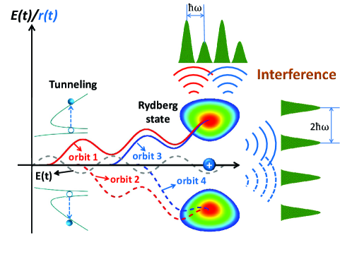
Figure 1: (color online). The Rydberg-state excitation process: The dashed gray curve denotes the laser electric field. The valence electron is liberated through tunneling in one of the various optical cycles of the pulse, whereupon it evolves in the laser field. The electrons captured into a certain Rydberg state in one direction (orbit 1 & orbit 3) or the other (orbit 2 & orbit 4) have different phases and will interfere, which leads to a peak structure in the intensity dependence with interval of $\Delta U_{p}=\hbar\omega$. Interference between the two directions leads to a peak structure with interval of $\Delta U_{p}=2\hbar\omega$ (see text for details).

II Quantum model

The transition amplitude of the capture process is given by (atomic units $m=\hbar=e=1$ are used)

$$M_{nlm}=\lim_{t\rightarrow\infty,t^{\prime}\rightarrow-\infty}\big{<}\Psi_{nlm}(t)|U(t,t^{\prime})|\Psi_{g}(t^{\prime})\big{>},$$ (1)

where $|\Psi_{nlm}\left(t\right)\rangle$ denotes a field-free Rydberg state with principal quantum number $n$, angular-momentum quantum number $l$, and magnetic quantum number $m$. $U(t,t^{\prime})$ denotes the time-evolution operator with the Coulomb and the laser fields wbecker1 , and $\Psi_{g}(\mathbf{r},t)=e^{iI_{p}t}\phi_{g}(\mathbf{r})$ indicates the wave function of the field-free ground state with the ionization potential $I_{p}$. It is assumed that the laser field is turned off in the distant past and future. The time-evolution operator $U(t,t^{\prime})$ satisfies the Dyson equation

$$U(t,t^{\prime})=U_{0}(t,t^{\prime})-i\int_{t^{\prime}}^{t}d\tau U(t,\tau)H_{I}(\tau)U_{0}(\tau,t^{\prime}),$$ (2)

where $U_{0}(t,t^{\prime})$ is the time-evolution operator for only the Coulomb field wbecker1 and (in length gauge) $H_{I}(t)=\textbf{r}\cdot\textbf{E}(t)$. With the help of Eq. (2), the transition amplitude (1) can be rewritten as

$$M_{nlm}= \lim_{t\rightarrow\infty}\Big{\{}\big{<}\Psi_{nlm}(t)|\Psi_{g}(t)\big{>}$$

$$-i\int_{-\infty}^{t}d\tau\big{<}\Psi_{nlm}(t)|U(t,\tau)H_{I}(\tau)|\Psi_{g}(\tau)\big{>}\Big{\}}.$$ (3)

Here, the first term on the right-hand side is zero due to the orthogonality of the Coulomb eigenstates. For the second term, we use a different form of the Dyson equation,

$$U(t,t^{\prime})=U_{V}(t,t^{\prime})-i\int_{t^{\prime}}^{t}d\tau U(t,\tau)VU_{V}(\tau,t^{\prime}),$$ (4)

where $V$ is the binding (Coulomb) potential and $U_{V}(t,t^{\prime})$ indicates the Volkov time-evolution operator

$$U_{V}(t,t^{\prime})=\int d^{3}\mathbf{k}|\Psi_{\mathbf{k}}^{(V)}(t)\rangle\langle\Psi_{\mathbf{k}}^{(V)}(t^{\prime})|,$$ (5)

which we have expanded in terms of the Volkov states with the wave functions

$$\Psi_{\mathbf{k}}^{(V)}(\mathbf{r},t)= \frac{1}{(2\pi)^{3/2}}\exp\Big{\{}i(\mathbf{k}+\mathbf{A}(t))\cdot\mathbf{r}$$

$$-\frac{i}{2}\int^{t}dt^{\prime}(\mathbf{k}+\mathbf{A}(t^{\prime}))^{2}\Big{\}},$$ (6)

where $\mathbf{k}$ denotes the asymptotic (drift) momentum. The coordinate-space representation of the Volkov time-evolution operator is

$$U_{V}(\mathbf{r}t,\mathbf{r}^{\prime}t^{\prime})=i\left(\frac{i}{2\pi(t-t^{\prime})}\right)^{\frac{3}{2}}e^{-iS(\mathbf{r}t,\mathbf{r}^{\prime}t^{\prime})}$$ (7)

with

$$S(\mathbf{r}t,\mathbf{r}^{\prime}t^{\prime})= \mathbf{A}(t)\cdot\mathbf{r}-\mathbf{A}(t^{\prime})\cdot\mathbf{r}^{\prime}+\frac{1}{2}\int^{t}_{t^{\prime}}d\tau\mathbf{A}^{2}(\tau)$$

$$-\frac{1}{2(t-t^{\prime})}\Big{[}\mathbf{r}-\mathbf{r}^{\prime}+\int^{t}_{t^{\prime}}d\tau\mathbf{A}(\tau)\Big{]}^{2}.$$ (8)

Using Eq. (4) in Eq. (II) we get

$$M_{nlm}= \lim_{t\rightarrow\infty}(-i)\int_{-\infty}^{t}d\tau\big{<}\Psi_{nlm}(t)|U_{V}(t,\tau)H_{I}(\tau)|\Psi_{g}(\tau)\big{>}$$

$$+\lim_{t\rightarrow\infty}(-i)^{2}\int_{-\infty}^{t}d\tau^{\prime}\int^{\tau^{\prime}}_{-\infty}d\tau$$

$$\times\big{<}\Psi_{nlm}(t)|U(t,\tau^{\prime})VU_{V}(\tau^{\prime},\tau)H_{I}(\tau)|\Psi_{g}(\tau)\big{>}.$$ (9)

This is analogous to the Born expansion of the ionization amplitude for above-threshold ionization. In that case, the final state is in the continuum and is approximated by a plane wave so that $\langle\Psi_{nlm}(t)|U_{V}(t,\tau)$ becomes a Volkov state $\langle\Psi_{\mathbf{p}}^{V}(\tau)|$. The first term then describes the direct electrons and the second term (with the exact propagator $U(t,t^{\prime})$ replaced by the Volkov propagator $U_{V}(t,t^{\prime})$) indicates single rescattering. For energies below $\approx 2U_{p}$, the first term is dominant. However, for RSE the first term in Eq. (5) goes to zero in the limit of $t\to\infty$. This is due to the factor of $(t-t^{\prime})^{-3/2}$ in Eq. (7), which accounts for wave-function spreading, and the fact that the Rydberg state $|\Psi_{nlm}(t)\rangle$ is localized. (Note that the values of $\tau$ in Eq. (II) are restricted to the finite duration of the laser pulse.) Hence, for RSE we only consider the second term.

In order to make further progress we replace the bra $\langle\Psi_{nlm}(t)|U(t,\tau^{\prime})$ in the second term by an approximate field-dressed Rydberg state with the wave function

$$\Psi_{nlm}^{d}(\mathbf{r},\tau^{\prime})=\phi_{nlm}(\mathbf{r})e^{-iE_{n}\tau^{\prime}}e^{i\mathbf{r}\cdot\mathbf{A}(\tau^{\prime})}e^{-i\int_{-\infty}^{\tau^{\prime}}d\tau A^{2}(\tau)/2},$$ (10)

where $\phi_{nlm}(\mathbf{r})$ is a field-free Rydberg state corresponding to the energy level $E_{n}=-1/(2n^{2})$. The principal quantum number, angular quantum number, and magnetic quantum number are indicated by $n$, $l$, and $m$, respectively. The field-free Rydberg states are given by

$$\phi_{nlm}(\mathbf{r}) =N_{nl}R_{nl}(r)Y_{lm}(\theta,\varphi),$$

$$N_{nl} =\frac{(2\kappa_{n})^{3/2}}{\Gamma(2l+2)}\sqrt{\frac{\Gamma(n+l+1)}{2n\Gamma(n-l)}},$$

$$R_{nl}(r) =(2\kappa_{n}r)^{l}e^{-\kappa_{n}r}\ _{1}F_{1}(-n+l+1,2l+2,2\kappa_{n}r),$$ (11)

where $\kappa_{n}=1/n$, $Y_{lm}(\theta,\varphi)$ is a spherical harmonic function, and ${}_{1}F_{1}(x,y,z)$ is the confluent hypergeometric function. The approximation (10), called the Coulomb-Volkov state, has been frequently used to account for the Coulomb-field in noncontinuum states; see Reiss1977 ; Jain1978 and many later references. The field-dressed state (10) does not exactly satisfy the Schrödinger equation. Namely, we have

$$i\frac{\partial}{\partial t}\Psi_{nlm}^{d}(\mathbf{r},t)= [E_{n}\phi_{nlm}(\textbf{r})+\frac{A^{2}(t)}{2}\phi_{nlm}(\textbf{r})+\mathbf{r}\cdot\mathbf{E}(t)\phi_{nlm}(\textbf{r})]$$

$$\times e^{-iE_{n}t}e^{i\mathbf{r}\cdot\mathbf{A}(t)}e^{-i\int_{0}^{t}\frac{A^{2}(\tau)}{2}d\tau},$$ (12)

and

$$[-\frac{1}{2}\nabla^{2}\!-\!\frac{1}{r}\!+\!\mathbf{r}\cdot\mathbf{E}(t)]\Psi_{nlm}^{d}(\mathbf{r},t)\!=\![E_{n}\phi_{nlm}(\textbf{r})\!-\!i\nabla\phi_{nlm}(\mathbf{r})\cdot\mathbf{A}(t)$$

$$+\!\frac{A^{2}(t)}{2}\phi_{nlm}(\textbf{r})\!+\!\mathbf{r}\cdot\mathbf{E}(t)\phi_{nlm}(\textbf{r})]e^{-iE_{n}t}e^{i\mathbf{r}\cdot\mathbf{A}(t)}e^{-i\int_{0}^{t}\frac{A^{2}(\tau)}{2}d\tau},$$ (13)

so that

$$\left[i\frac{\partial}{\partial t}+\frac{1}{2}\mbox{\boldmath$\nabla$}^{2}+\frac{1}{r}-\mathbf{r}\cdot\mathbf{E}(t)\right]\Psi_{nlm}^{d}(\mathbf{r},t)$$

$$=ie^{-iE_{n}t}e^{i\mathbf{r}\cdot\mathbf{A}(t)}e^{-i\int_{0}^{t}\frac{A^{2}(\tau)}{2}d\tau}\mathbf{A}(t)\cdot\mbox{\boldmath$\nabla$}\phi_{nlm}(\mathbf{r}).$$ (14)

Hence, the approximation (10) would be exact if it were not for the term $-i\nabla\phi_{nlm}(\textbf{r})\cdot A(t)$ on the right-hand side of Eq. (14). A comparison of the four terms of Eq. (13) is shown in Table I. It can be seen that the disturbing term $\nabla\phi_{nlm}(\textbf{r})$ is several orders smaller than the other three terms in the region where the Rydberg state is concentrated (see Figs. 3 and 8 in the appendix) for the times of capture (for details, see the semiclassical analysis part of the appendix) shown in Fig. 2. Therefore, Eq. (10) can be considered a good approximation to the dressed Rydberg state, and our final approximation to the Rydberg-capture amplitude is

$$M_{nlm} =\!(-i)^{2}\!\int^{\infty}_{-\infty}\!dt\!\int^{t}_{-\infty}\!dt^{\prime}\!\langle\Psi^{d}_{nlm}(t)|VU_{V}(t,t^{\prime})H_{I}(t^{\prime})|\Psi_{g}(t^{\prime})\rangle$$

$$=(-i)^{2}\int_{-\infty}^{\infty}dt\int_{-\infty}^{t}dt^{\prime}\int d^{3}\mathbf{k}$$

$$\times\langle\Psi_{nlm}^{d}(t)|V(\mathbf{r})|\Psi_{\mathbf{k}}^{(V)}(t)\rangle\langle\Psi_{\mathbf{k}}^{(V)}(t^{\prime})|\mathbf{r^{\prime}}\cdot\mathbf{E}(t^{\prime})|\Psi_{g}(t^{\prime})\rangle.$$ (15)

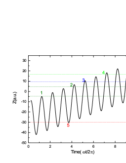
Figure 2: A typical trajectory of the electron in the laser pulse with intensity of $1\times 10^{14}$ W/cm². The numbers indicate the instants of time $t$ when the electron is captured by the Rydberg states of $n=6$ of the hydrogen atom with different angular momenta.

Table 1: Relative amplitudes of the four terms of Eq. (13). The quantities $t$ and $l$ indicate the capture moment and the angular momentum number shown in Fig. 2, respectively.

	$t$	$l$	E${}_{n}(n=6)$	$\frac{\nabla\phi_{nlm}(r)}{\phi_{nlm}(r)}\cdot\mathbf{A}(t)$	$\frac{A^{2}(t)}{2}$	$\mathbf{r}\cdot\mathbf{E}(t)$
	1	2	-0.014	$-2.47\times 10^{-7}$	0.009	0.20
	2	2	-0.014	$-9.91\times 10^{-7}$	0.147	0.35
	3	3	-0.014	$-3.62\times 10^{-7}$	0.102	0.44
	4	4	-0.014	$-4.16\times 10^{-6}$	0.129	0.75
	5	5	-0.014	$2.21\times 10^{-6}$	0.080	-1.45

With the help of Eqs. (7), (10), and the binding potential $V(r)=-1/r$, the capture amplitude (15) has the following form

$$M_{nlm}\!=\!(-i)^{2}\!\int_{-\infty}^{\infty}\!dt\!\int_{-\infty}^{t}\!dt^{\prime}\!\int d^{3}\!\mathbf{k}\!V_{nlm,\mathbf{k}}\!V_{\mathbf{k}g}\!\exp[iS_{n}(t,t^{\prime},\mathbf{k})],$$ (16)

with

$$V_{\mathbf{k}g} =\!\frac{1}{(2\pi)^{3/2}}\!\int d^{3}\!\mathbf{r^{\prime}}\exp\{-i[\mathbf{k+A}(t^{\prime})]\cdot\mathbf{r^{\prime}}\}\mathbf{r}^{\prime}\cdot\mathbf{E}(t^{\prime})\psi_{g}(\mathbf{r^{\prime}})$$

$$=\!\frac{1}{(2\pi)^{3/2}}\!(-i\frac{\partial}{\partial t^{\prime}})\int d^{3}\mathbf{r^{\prime}}\exp\{-i[\mathbf{k+A}(t^{\prime})]\cdot\mathbf{r^{\prime}}\}\psi_{g}(\mathbf{r^{\prime}}).$$ (17)

$$V_{nlm,\mathbf{k}}=-\frac{1}{(2\pi)^{3/2}}\int d^{3}\mathbf{r}\phi^{*}_{nlm}(\mathbf{r})\frac{1}{r}\exp(i\mathbf{k}\cdot\mathbf{r}),$$ (18)

and the action

$$S_{n}\!\left(t,t^{\prime},\mathbf{k}\right)\!=\!\frac{1}{2}\!\int^{t}_{-\infty}\!d\tau\!\mathbf{A}^{2}\left(\tau\right)-\frac{1}{2}\!\int_{t^{\prime}}^{t}\!d\tau\!\left[\mathbf{k+A}\left(\tau\right)\right]^{2}+E_{n}t+I_{p}t^{\prime}.$$

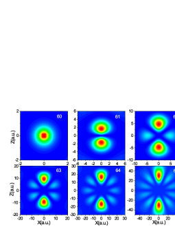
Figure 3: Density distribution of the hydrogenic Rydberg state $n=6$ for different angular quantum numbers $l$. The two numbers in each panel correspond to the principal quantum number $n$ and the angular-momentum quantum number $l$.

In Fig. 3, the probability densities of the relevant Rydberg states are plotted for $n=6$ and different values of $l$. It can be easily seen that for $l\neq 0$ the Rydberg state has two centers at $\mathbf{r}_{nlm}^{+}\equiv\mathbf{r}_{nlm}$ and $\mathbf{r}_{nlm}^{-}=-\mathbf{r}_{nlm}^{+}\equiv-\mathbf{r}_{nlm}$. Accordingly, we decompose the Rydberg-state wave function as

$$\phi_{nlm}(\mathbf{r})=\phi_{nlm+}(\mathbf{r})+\phi_{nlm-}(\mathbf{r}),$$ (19)

where the functions $\phi_{nlm\pm}(\mathbf{r})$ are concentrated around $\mathbf{r}=\pm\mathbf{r}_{nlm}$. Also, $\phi_{nlm-}(-\mathbf{r})=(-1)^{l}\phi_{nlm+}(\mathbf{r})$, which allows us to write

$$V_{nlm,\mathbf{k}} =-\frac{1}{(2\pi)^{3/2}}\int\frac{d^{3}\mathbf{r}}{r}\left[\phi^{*}_{nlm+}(\mathbf{r})e^{i\mathbf{k}\cdot\mathbf{r}}+\phi^{*}_{nlm-}(\mathbf{r})e^{i\mathbf{k}\cdot\mathbf{r}}\right]$$

$$=-\frac{1}{(2\pi)^{3/2}}\int\frac{d^{3}\mathbf{r}}{r}\left[\phi^{*}_{nlm+}(\mathbf{r})e^{i\mathbf{k}\cdot\mathbf{r}}+\phi^{*}_{nlm-}(-\mathbf{r})e^{-i\mathbf{k}\cdot\mathbf{r}}\right]$$

$$=-\frac{1}{(2\pi)^{3/2}}\int\frac{d^{3}\mathbf{r}}{r}\phi^{*}_{nlm+}(\mathbf{r})\left[e^{i\mathbf{k}\cdot\mathbf{r}}+(-1)^{l}e^{-i\mathbf{k}\cdot\mathbf{r}}\right].$$ (20)

With the abbreviation $\phi_{nlm+}(\mathbf{r})=\phi_{nlm+}(\mathbf{r}-\mathbf{r}_{nlm}+\mathbf{r}_{nlm})\equiv\tilde{\phi}_{nlm}(\rho)$, where $\rho=\mathbf{r}-\mathbf{r}_{nlm}$, we end up with

$$V_{nlm,\mathbf{k}} =-\frac{1}{(2\pi)^{3/2}}\int d^{3}\bm{\rho}\frac{1}{|\bm{\rho}+\mathbf{r}_{nlm}|}\tilde{\phi}_{nlm}^{*}(\bm{\rho})\Big{[}e^{i\mathbf{k}\cdot\bm{\rho}}e^{i\mathbf{k}\cdot\mathbf{r}_{nlm}}$$

$$+(-1)^{l}e^{-i\mathbf{k}\cdot\bm{\rho}}e^{-i\mathbf{k}\cdot\mathbf{r}_{nlm}}\Big{]}.$$ (21)

We can now proceed with the saddle-point evaluation as it is usually done by including the fast exponential dependence generated by the factors $\exp(\pm i\mathbf{k}\cdot\mathbf{r}_{nlm})$ into the action while treating the remaining $\mathbf{k}$ dependence as slow. This means that we replace

$$V_{nlm,\mathbf{k}}e^{iS_{n}(t,t^{\prime},\mathbf{k})} =V_{nlm,\mathbf{k}+}e^{i\big{[}S_{n}(t,t^{\prime},\mathbf{k})+\mathbf{k}\cdot\mathbf{r}_{nlm}\big{]}}$$

$$+(-1)^{l}V_{nlm,\mathbf{k}-}e^{i\big{[}S_{n}(t,t^{\prime},\mathbf{k})-\mathbf{k}\cdot\mathbf{r}_{nlm}\big{]}},$$ (22)

where

$$V_{nlm,\mathbf{k}\pm}=-\frac{1}{(2\pi)^{3/2}}\int d^{3}\bm{\rho}\tilde{\phi}^{*}_{nlm}(\bm{\rho})\frac{1}{|\bm{\rho}+\mathbf{r}_{nlm}|}e^{\pm i\mathbf{k}\cdot{\bm{\rho}}}.$$ (23)

Then, we search for those values of the variables $t$, $t^{\prime}$, and $\mathbf{k}$ that render the action $S_{n}\pm\mathbf{k}\cdot\mathbf{r}_{nlm}$ stationary, which yields, in turn,

$$[\mathbf{k}+\mathbf{A}(t^{\prime})]^{2}/2 =-I_{p},$$ (24)

$$[\mathbf{k}+\mathbf{A}(t)]^{2}/2 =A^{2}(t)/2+E_{n},$$ (25)

$$\mathbf{k}_{\textrm{st}}^{\pm}=-\frac{1}{t-t^{\prime}}\int^{t}_{t^{\prime}} d\tau\mathbf{A}(\tau)\pm\frac{\mathbf{r}_{nlm}}{t-t^{\prime}}=\mathbf{k}_{0}\pm\frac{\mathbf{r}^{+}_{nlm}}{\tau},$$ (26)

where $\mathbf{k}_{0}=-\frac{1}{t-t^{\prime}}\int^{t}_{t^{\prime}}d\tau\mathbf{A}(\tau)$ and $\tau=t-t^{\prime}$. Equations (24) and (25) describe, respectively, energy conservation in the tunneling process and in the capture process, while Eq. (26) determines the intermediate electron momentum. The latter takes into account that the electron is captured at one of the two positions $\pm\mathbf{r}_{nlm}$. The solutions $(t,t^{\prime},\mathbf{k})$ of Eqs. (24)–(26) define the quantum orbits.

Throughout the paper, we will refer to Eq. (15) as the quantum model (QM), and the multiple integrals are performed by numerical integration with respect to $t$ and $t^{\prime}$ and by saddle-point integration with respect to k. At the end of the pulse, the population of the $n$th Rydberg state is defined as $P_{n}=\sum_{l,m}|M_{nlm}|^{2}$. In our simulation, magnetic quantum number $m=0$ and (field-free) energy $E_{n}=-1/(2n^{2})$ are adopted. The ten-cycle laser electric field is $\mathbf{E}(t)=E_{0}\sin\omega t\mathbf{\hat{e}_{z}}$ with the vector potential $\mathbf{A}(t)=E_{0}/\omega\cos\omega t\mathbf{\hat{e}_{z}}$ ($\mathbf{\hat{e}_{z}}$ is a unit polarization vector and the wavelength $\lambda=2\pi c/\omega=800$ nm). The 1$s$ atomic orbital is expressed as $\phi_{1s}(\mathbf{r})=\frac{1}{\sqrt{\pi}}\kappa^{3/2}e^{-\kappa r}$ with $\kappa=\sqrt{2I_{p}}$. For Xe(5$p$), $\phi_{5p}(\mathbf{r})=\frac{(2\xi)^{11/2}}{\sqrt{10!}}\sqrt{\frac{3}{4\pi}}r^{4}e^{-\kappa r}\cos\theta$ with $\xi=0.65\sqrt{2I_{p}}$ and $\kappa=0.94\sqrt{2I_{p}}$. The ionization potential of the H, He, and Xe atoms are 0.5 a.u., 0.9 a.u., and 0.44 a.u., respectively. For the TDSE simulation, the details can be found in Ref. lin2014PRA .

III Results and discussions

I. Comparison of TDSE and model calculations

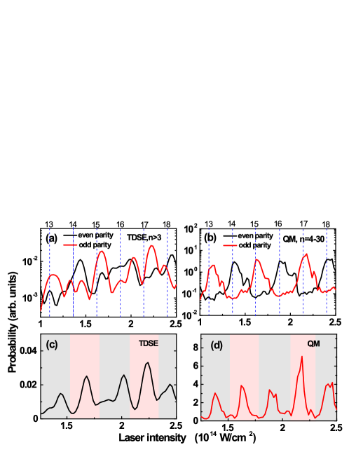
Figure 4: (color online). Populations of Rydberg states with even or odd parity versus laser intensity calculated via TDSE (a) and the quantum model (QM)(b) for an initial 1$s$ state. The positions of the $N$-photon channel closings are indicated on the top $x$ axis. For visual convenience, the peaks are separated by dashed lines and underlaid with alternatingly gray or pink backgrounds. Total Rydberg-state populations on a linear scale (sum over parities) as functions of the laser intensity simulated by (c): the TDSE and (d): the QM for an initial 1$s$ state.

In Figs. 4(a) and 4(b), we show the probability of Rydberg states with principal quantum numbers $n>3$ and with opposite parities of the final Rydberg states ($l$ even or odd) calculated by the TDSE and the quantum model for an initial $1s$ state of the H atom as functions of the laser intensity. (For the TDSE, the pulse envelope is given by a cosine square function with full width at half maximum of 10 fs, and the details of the simulation can be found in lin2014PRA ). Peaks separated by an intensity interval of about 25 TW/cm², corresponding to a shift of the ponderomotive energy $U_{p}$ by the energy of a laser photon, i.e., $\Delta U_{p}=\hbar\omega$ ($\approx 1.55$ eV), can be clearly seen in Fig. 4 for both the TDSE and the quantum model calculation. The results of the quantum model are almost quantitatively consistent with the TDSE results except for a small shift of the peaks. In particular, for initial states and Rydberg states with specified parities, two consecutive peaks are separated by about $\Delta U_{p}=2\hbar\omega$. These obvious quantum features can be easily understood in the multiphoton transition picture of RSE voklova2010JETP ; Freeman1987PRL . Since the energies of the Rydberg states are near the threshold so that their Stark shifts are all close to the Stark shift $U_{p}$ of the continuum, multiphoton resonance between the Rydberg and the initial states occurs at intensities that are separated by $\Delta U_{p}=\hbar\omega$ Freeman1987PRL . In addition, the dipole selection rule only allows even-order (odd-order) multiphoton transitions between states of equal (opposite) parity, which gives rise to a $\Delta U_{p}=2\hbar\omega$ separation between consecutive peaks for a transition between two states with specified parity lin2014PRA ; Piraux2017PRA . Apparently, these features are beyond the scope of the semiclassical picture of the RSE.

Furthermore, closer inspection shows that the peaks alternate in height as shown in Figs. 4(c) and 4(d), which display the population of the Rydberg states with both parities. This can also be observed in the results of Refs. voklova2010JETP ; lin2014PRA ; ZPIE2017 though it was not addressed there. This feature is difficult, if not impossible, to understand in the multiphoton-resonance picture. For a transition from the ground state to the Rydberg state, the electron has to absorb more than ten photons under typical laser conditions as considered here ($\hbar\omega=1.55$ eV and $U_{p}=6$ eV for $I=1\times 10^{14}$ W/cm²). The density of the Rydberg states does not depend on the parity. Hence, no mechanism such as a selection rule can give rise to a structure that depends on whether an even or odd number of photons is absorbed in the process.

II. Analysis of the quantum model

In order to elucidate these intriguing features, we classify the quantum orbits in our model according to the length of their travel time, that is, the time difference $\Delta t=t-t^{\prime}$ between recapture and ionization. Specifically, with the number $J$ we denote the pair of orbits where $(J-1)T/2<\Delta t<JT/2$ where $T=2\pi/\omega$. We call an orbit even or odd according to whether $J$ is even or odd. Figure 5(a) shows the results calculated using Eq. (15) for the Rydberg state $n=6$ and $l=5$ for different electronic orbits. We take the Rydberg state $n=6$, since for this state the calculated results show a maximum in our laser intensity range NISS2009 ; lin2014PRA . We notice that the intensity dependence is a straight line for the orbit with $J=20$. For $J=18$, an oscillatory structure is beginning to develop, which becomes more and more apparent when $J$ becomes smaller (not shown here). Finally, for $J=1$ and 2, pronounced peaks have emerged. This is because the total pulse duration used in our calculation is $10\,T$. Namely, for the orbit with $J=20$ the electron must be freed in the earliest half cycle while for orbits with smaller $J$ electrons liberated during more and more subsequent half cycles contribute and interfere with each other, which results in the peak structure. Hence, the peak structure in the intensity dependence of the RSE can be attributed to interference between electron wave packets generated in different optical half cycles during the laser pulse, which is in agreement with Ref. ZPIE2017 .

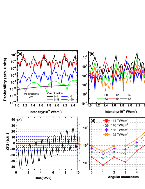
Figure 5: (color online). (a): Interference pattern generated by orbits with different values of $J$ as given (see text for details). (b): The population of RSE for different $l$ for a fixed principal quantum number $n=6$ in an 800-nm laser field. (c): The electron trajectory in the field $\mathbf{E}(t)=E_{0}\sin\omega t\mathbf{e}_{z}$ corresponding to ionization at the phase $\omega t_{0}=92^{\circ}$after the field maximum. The laser intensity is $1.14\times 10^{14}$ W/cm² and the transverse velocity is 0 a.u. The colored horizontal dashed lines indicate the boundaries (in the coordinate $z$) of those regions where the Rydberg states with $n=6$ and $l\leq 5$ have their highest density as shown in Fig. 8 below. (d): The populations of specific $l$ within the semiclassical picture for $n=6$ at four different peak intensities (see the text for details).

For a closer look, we consider Fig. 1. For a sufficiently long (i.e., almost perodic) laser pulse, the ionization dynamics triggered by this pulse repeat themselves from one cycle to the next (see, e.g., orbits 1 and 3). Following a similar analysis in Ref. Milosev2007 , if a saddle point solving Eqs. (24) - (26) with the Rydberg-state recombination site in the positive direction [+ sign in Eq. (26)] is given by $(\mathbf{k},t,t^{\prime})$, then the saddle point in the next optical cycle with the same Rydberg state in the same direction is $(\mathbf{k},\,t+T,\,t^{\prime}+T)$, and the corresponding action is related by

$$S_{n}(t+T,t^{\prime}+T,\mathbf{k})=S_{n}(t,t^{\prime},\mathbf{k})+(E_{n}+I_{p}+U_{p})T.$$ (27)

So the contributions of these trajectories differ by the phase $(U_{p}+I_{p}+E_{n})T=(U_{p}+I_{p}+E_{n})2\pi/\omega$ (orbits 1 and 3). The same holds true for orbits 2 and 4, half a period later when the field has changed sign. Due to parity symmetry, a Rydberg state (except for $l=0$) has two opposite density maxima in the field direction, and the electron can be captured into one or the other. In the figure, orbits 1 and 3 go into one direction and orbits 2 and 4 into the other. If a saddle point solving Eqs. (24) - (26) with the Rydberg-state recombination location in the positive direction [+ sign in Eq. (26)] is written as $(\mathbf{k},t,t^{\prime})$, then the saddle point solving these equations with the same recombination location in the negative direction [- sign in Eq. (26)] is $(-\mathbf{k},\,t+T/2,\,t^{\prime}+T/2)$, and the corresponding action is given by

$$S_{n}(t+T/2,t^{\prime}+T/2,-\mathbf{k})=S_{n}(t,t^{\prime},\mathbf{k})+(E_{n}+I_{p}+U_{p})T/2.$$ (28)

So the contributions of 2 and 4 differ from those of 1 and 3 by the phase $(U_{p}+I_{p}+E_{n})T/2=(U_{p}+I_{p}+E_{n})\pi/\omega$. The interference of the contributions of orbits 1 and 2 with those of orbits 3 and 4, i. e., the contributions of two directions, gives rise to peaks in the RSE separated by $\Delta U_{p}=2\hbar\omega$, while the afore-mentioned periodicity from cycle to cycle yields peaks with the separation of $\Delta U_{p}=\hbar\omega$, which is common for all interferences in a field with period $T$. These two kinds of interference can be clearly seen in Fig. 5(a).

Another element to be considered are the phases due to the parities of the initial ground state and the final Rydberg state, which are $(-1)^{p}$ with $p=\pm 1$ the respective parities. Hence, if the initial and the final state have opposite parities, an additional phase of $\pi$ occurs. We notice that the interference between quantum orbits that are recaptured in opposite directions of the same Rydberg state plays the same role in the quantum model as the selection rule does in the multiphoton transition picture.

It is noteworthy that the peaks in Figs. 4(b) and 4(d) also closely satisfy the channel-closing (CC) condition $I_{p}+U_{p}=m\omega$. For example, the two peaks at $1.16\times 10^{14}$ W/cm² and $1.42\times 10^{14}$ W/cm² in Fig. 4(b) correspond to $U_{p}=6.9$ and 8.5 eV and, with the ionization potential $I_{p}=13.6$ eV and the negligible ionization potential of the highly excited Rydberg state, satisfy the CC condition for $m=13$ and $m=14$, in agreement with the Freeman resonance picture and the selection rule.

From the above analysis, as schematically illustrated in Fig. 1 and elaborated above, we find that there are essentially two types of interference of the quantum orbits in the excitation of a Rydberg state with specific $n$ and $l$ from the ground state: i) interference of wave packets released during different optical cycles and captured in one and the same half of the spatial region of the Rydberg state gives rise to peaks separated by a laser intensity difference corresponding to $\Delta U_{p}=\hbar\omega$; ii) interference of orbits released in adjacent half cycles (and captured in opposite spatial regions of the Rydberg state) results in a peak structure with intensity difference corresponding to $\Delta U_{p}=2\hbar\omega$, and the peak positions depending on the relative parity of the Rydberg and the ground states.

Figure 5(b) displays the population of different orbital angular momenta $l$ for $n=6$. In the intensity range from $1\times 10^{14}$ W/cm² to $2.5\times 10^{14}$ W/cm² the Rydberg states with $l=4$ and 5 are predominantly populated. The maximal populations of $l=4$ and 5 as a function of laser intensity correspond to the low and high peaks in Figs. 4(b) and 4(d), respectively.

For a different view of these features, we now turn to a semiclassical picture (see the Appendix for the details). In Fig. 5(c), we present an example of an electron trajectory for ionization at $\omega t_{0}=92^{\circ}$ with zero initial longitudinal and transverse velocity. We assume that the probability of capture into the Rydberg state $(n,l,m)$ is maximal if the electron trajectory $(X(t),Z(t))$ passes the spatial region where its density $|\phi_{nlm}(\mathbf{r})|^{2}$ is highest at a time where its kinetic energy is very low. We determine this spatial region from a graph of the Rydberg-state wave function (see Fig. 8 of the Appendix). For the kinetic energy we require $E_{\mathrm{kin}}<0.05$ a.u., and there are two time domains which satisfy the capture condition for every optical cycle (see Fig. 7 of the Appendix). Figure 5(d) displays the angular-momentum distributions obtained this way. Clearly, regardless of intensity $l=5$ dominates all other angular momenta, which is in reasonable agreement with the results of the QM model in Fig. 5(b). In addition, it can be seen that the population of $l=5$ for 166 TW/cm² is higher than that of $l=4$ for 192 TW/cm² and also for 140 TW/cm², which confirms the alternating heights of the peaks in the quantum model displayed by Fig. 5(b). Therefore, the alternating heights of the RSE peaks shown in Fig. 4 are already engrained in this “simple-man model”. It should be noted that even though the population at 114 TW/cm² is higher than that of 140 TW/cm² in Figs. 5(b) and 5(d), this is not the case for the total population shown in Figs. 4(a) and 4(b). This can be attributed to the fact that the relative contributions from other Rydberg states with different $n$ change and affect the modulation when the intensity is low.

III. Comparison with experiments

Experiments show that for the He atom the population of the Rydberg states peaks at about $n=9$ at $I=1.8\times 10^{15}$ W/cm² with a slight tendency to shift to higher $n$ when the intensity increases to $I=2.9\times 10^{15}$ W/cm² Eichmann2015PRL . For comparison, the focal average of the RSE calculated by our proposed quantum model is shown in Fig. 6(a) which shows that the maximum of the RSE shifts to higher energy for increasing intensity, in qualitative agreement with the experiment. For fixed-intensity RSE yields, however, our quantum model shows a reverse intensity dependence (see Fig. 6(b)), which reproduces the results of TDSE simulations lin2014PRA . This apparent conflict can be resolved as follows: According to the physical picture underlying our quantum model, the electron after tunneling out from the ground state oscillates in the laser field while drifting towards the detector. When it reaches the position of the Rydberg state, provided its instantaneous kinetic energy is very low, it can be captured (see the typical orbits in Fig. 1). Therefore, for small drift momentum, it can be expected that the RSE yield becomes maximal around principal quantum numbers $n$ roughly given by $n^{2}\approx 4\sqrt{U_{p}}/\omega$, so that the yield slightly shifts with increasing intensity as shown in Fig. 6(a). The positions of the maxima of the RSE yields in the fixed-intensity results of Fig. 6(b) and Ref. lin2014PRA are determined by interference as was shown above. However, interference effects are largely smeared out by focal averaging, which restores agreement with the TDSE and the semiclassical calculations in Ref. Eichmann2015PRL . It should be noted that this $n$ distribution cannot be explained by the Freeman resonance mechanism.

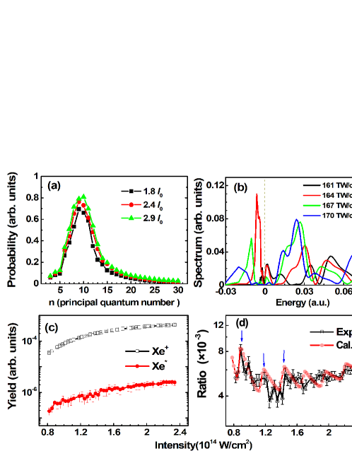
Figure 6: (color online). (a): Focal-averaged RSE vs. principal quantum number calculated by the quantum model for the He atom, for $I_{0}=10^{15}$ W/cm²; (b): Calculated electron spectra below (multiplied by a factor of 0.2) and above the continuum threshold for the hydrogen atom and various fixed intensities; (c): Experimental yields of single ionization and RSE of the Xe atom; (d): Experimental and calculated ratios between the Rydberg excitation and the single ionization yields (see the text for more detail).

Moreover, we experimentally measured the single-ionization yields and the RSE of the Xe atom for principal quantum numbers between $n=20$ and $n=30$. The experimental setup is introduced in Ref. Lv2016PRA (see the Appendix for more details). The results for Xe are presented in Figs. 6(c) and 6(d). The intensity-dependent ionization yield follows a smooth curve. However, the RSE yield does display some peak structure especially in the low intensity regime below $I=1.5\times 10^{14}$ W/cm² [see Fig. 6(c)]. This is especially evident in the ratio Xe^∗/Xe⁺, which exhibits peaks at $I_{1}=0.89\times 10^{14}$ W/cm², $I_{2}=1.18\times 10^{14}$ W/cm², and $I_{3}=1.45\times 10^{14}$ W/cm² [see the blue arrows in Fig. 6(d)]. This structure is qualitatively reproduced by the quantum model if focal averaging is included, indicating that this structure is the remainder of the peak structure after taking into account the intensity distribution in the focus.

IV Conclusions and Perspectives

In summary, we propose a new quantum model based in the spirit of the SFA to study the RSE process in an intense infrared laser field. In this quantum model, the electron is first pumped by the laser field into the continuum where subsequently it evolves in the laser field. Most of the liberated electrons end up as free electrons (ATI); however, some may be captured into a Rydberg state. The electronic wave packets liberated in different optical half cycles are responsible for peak structures in the intensity dependence of the RSE yield. The peaks exhibit a modulation, which can be attributed to a strong dependence of the capture probability on the spatial position and the parity of the Rydberg state. Our calculation also well reproduces the experimentally observed atomic RSE distribution and the intensity dependence of RSE of atoms. The quantum picture of the RSE in an intense laser field can be understood as a coherent recapture process accompanying above-threshold ionization.

We expect similar quantum effects for molecules. For example, RSE of the O₂ molecule is suppressed compared with that of its companion atom Xe, and this suppression is stronger than the corresponding suppression of ionization of O₂ compared with that of Xe Lv2016PRA . Apparently, this cannot be described by the semiclassical model. Another such example will be two-center interference, which has been accepted to be essential in molecular ionization Becker2000PRL ; lin2012PRL . With some extensions, our quantum model can be applied to investigate these intriguing phenomena and reveal the underlying physics. Work along these lines is in progress.

V Acknowledgment

The authors acknowledge Xiaojun Liu for helpful discussions. This work was supported by the National Key program for S&T Research and Development (No. 2016YFA0401100), NNSFC (Nos. 11804405, 11425414, and 11534004), and Fundamental Research Fund of Sun Yat-Sen University (18lgpy77).

VI APPENDIX:  Semiclassical analysis and experimental technique

Semiclassical analysis

In the simpleman picture where the ionic Coulomb potential is ignored, the equation of motion of the electron in the laser field after ionization is

$$\ddot{\mathbf{r}}(t)=-\mathbf{E}(t).$$ (A1)

Here the electric field is $\mathbf{E}(t)=E_{0}\sin\omega t\mathbf{\hat{e}_{z}}$ with the vector potential $\mathbf{A}(t)=E_{0}/\omega\cos\omega t\mathbf{\hat{e}_{z}}$ ($\mathbf{\hat{e}_{z}}$ is a unit polarization vector), and the wavelength is $\lambda=$ 800 nm. The electron trajectory in the laser field starts at the tunnel exit $z_{0}=-I_{p}/E(t_{0})$ with zero longitudinal and nonzero initial transverse velocity $\mathbf{v}(t_{0})=(0,v_{0})$. If we integrate the equation of motion, we obtain

$$dz(t)/dt= A(t)-A(t_{0}),$$

$$dx(t)/dt= v_{0}.$$

Integrating again we get the trajectory of the electron:

$$z(t) =z(t_{0})-A(t_{0})(t-t_{0})+\int^{t}_{t_{0}}A(\tau)d\tau$$

$$=\!-\frac{I_{p}}{E_{0}\sin\omega t_{0}}\!-\!\frac{E_{0}}{\omega}\cos\omega t_{0}(t\!-\!t_{0})\!+\!\frac{E_{0}}{\omega^{2}}(\sin\omega t\!-\!\sin\omega t_{0}),$$

$$x(t) =v_{0}(t-t_{0}).$$

The semiclassical physical picture of the RSE can be summarized as follows: the electron is released at the time $t_{0}$ into a continuum Volkov state. Subsequently, it evolves in the laser field and can be captured into the Rydberg state at time $t$ provided (i) it reaches the spatial region where the Rydberg state has a high density (here we use the condition $|\phi|^{2}>0.8|\phi|^{2}_{\textrm{max}}$) and (ii) its kinetic energy $E_{kin}$ is small (here we use $E_{kin}\leqslant 0.05$ a.u.). It should be noted that the result is not sensitive to these criteria.

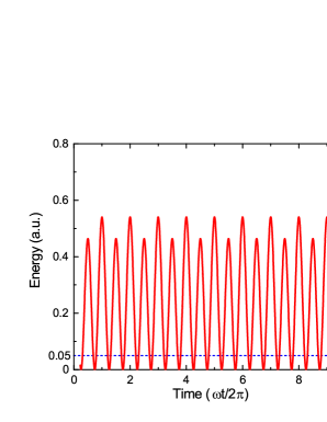
Figure 7: Kinetic energy of the electron during its evolution in a laser pulse of 10 optical cycles. The laser intensity is $1.14\times 10^{14}$ W/cm², and the initial phase and the transverse velocity are 92^∘ and 0, respectively.

In Fig. 7, we show the evolution of the kinetic energy of the electron under the given initial conditions and parameters. It can be seen that there are two time intervals in each optical cycle where the kinetic energy is small enough for capture, i. e., $E_{kin}\leqslant 0.05$ a.u., as defined above.

For Rydberg states of $n=6$ and different values of $l$ (see Fig. 3), Fig. 8 identifies for these $l$ the regions where the density criterion $|\phi|^{2}>0.8|\phi|^{2}_{\textrm{max}}$ is satisfied. Clearly, the relevant region moves towards larger distances from the origin with increasing $l$.

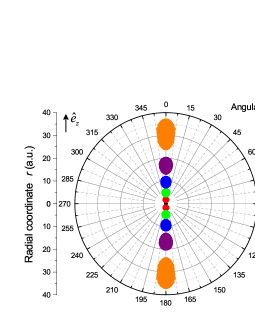
Figure 8: The regions in polar coordinates where the Rydberg-state densities $|\phi_{nlm}(\mathbf{r})|^{2}$ are larger than 80 percent of their maximal values for $n=6$ and angular momenta $l\leq n-1$. Different colors denote different angular momenta.

In our calculation, each electron trajectory is released via tunneling at some instant during the laser-pulse duration (a 10-cycle pulse with constant electric amplitude is considered). Its weight, which is dependent on the ionization rate and the initial transverse velocity (from -0.3 a.u. to 0.3 a.u.), is determined as in Ref. NISS2009 . Then the electron evolves in the laser field until the end of the laser pulse. If it reaches the regions shown in Fig. 8 and its kinetic energy is smaller than 0.05 a.u., it is considered to be captured by the Rydberg state $\phi_{nlm}$. The final Rydberg excitation probabilities shown in Fig. 5(d) of the main body of the paper are obtained from statistic of all the trajectories satisfying the afore-mentioned criteria of capture (about 10⁴-10⁶ trajectories for each state depending on $l$) in overall 2$\times 10^{7}$ trajectories.

Experimental technique

In our experiments, we applied the delayed-static-field-ionization method to ionize the neutral Rydbergs, using a time-of-flight (ToF) mass spectrometer operated under a pulsed-electric-field mode. Experimentally, an effusive atomic or molecular beam through a leak valve interacted with a focused Ti:Sapphire femtosecond laser with a central wavelength of 800 nm and pulse duration of 50 fs. After the direct-ionized ions (Xe⁺) were pushed away from the detector by an electric field, the remaining high-lying neutral Rydbergs (Xe^∗) were field-ionized by another electric field with a delay time of typically 1.0 $\mu$s, and were detected by dual micro-channel plates at the end of the flight section of about 50 cm. In the case of detection of Xe⁺, standard dc electric fields were applied in the ToF mass spectrometer. The voltages in both cases were kept the same to ensure identical detection efficiencies for Xe⁺ and (Xe^∗)⁺. This allows us to detect the neutral Rydberg states with $20<n<30$, estimated by the saddle-point model of static-field ionization $[F=1/(9n^{4})]$. The laser-pulse energy was controlled by a half-wave plate and a Glan prism, before being focused into the vacuum chamber with a 250 mm lens. The peak intensity of the focused laser pulse was calibrated by comparing the measured saturation intensity of Xe with that calculated by the ADK model ADK . The scanning of the laser intensity was precisely controlled by simultaneously monitoring the pulse energy using a fast photodiode while rotating the half-wave plate. Each data point was an averaged result of $10^{4}$ laser shots with an intensity uncertainty of 1 TW/cm².

References

- (1) R. R. Freeman, P. H. Bucksbaum, H. Milchberg, S. Darack, D. Schumacher, and M. E. Geusic, Above-threshold ionization with subpicosecond laser pulses, Phys. Rev. Lett. 59, 1092 (1987).
- (2) H. G. Muller, H. B. van Linden van den Heuvell, P. Agostini, G. Petite, A. Antonetti, M. Franco, and A. Migus, Multiphoton ionization of Xenon with 100-fs Laser Pulses, Phys. Rev. Lett. 60, 565 (1988).
- (3) R. R. Jones, D. W. Schumacher, and P. H. Bucksbaum, Population trapping in Kr and Xe in intense laser fields, Phys. Rev. A 47, R49 (1993).
- (4) H. Rottke, B. Wolf-Rottke, D. Feldmann, K. H. Welge, M. Dörr, R. M. Potvliege, and R. Shakeshaft, Atomic hydrogen in a strong optical radiation field, Phys. Rev. A 49, 4837 (1994).
- (5) P. Agostini, F. Fabre, G. Mainfray, G. Petite, and N. K. Rahman, Free-free transitions following six-photon ionization of xenon atoms, Phys. Rev. Lett. 42, 1127 (1979).
- (6) For a review, see, e.g., W. Becker, F. Grasbon, R. Kopold, D. B. Milošević, G. G. Paulus, and H. Walther, Above-threshold ionization: from classical features to quantum effects, Adv. At. Mol. Opt. Phys. 48, 35 (2002).
- (7) W. Becker, X. Liu, P. Ho, and J. H. Eberly, Theories of photoelectron correlation in laser-driven multiple atomic ionization, Rev. Mod. Phys. 84, 1011 (2012).
- (8) B. B. Wang, X. F. Li, P. M. Fu, J. Chen, and J. Liu, Coulomb potential recapture effect in above-barrier ionization in laser pulses, Chin. Phys. Lett. 23, 2729 (2006).
- (9) T. Nubbemeyer, K. Gorling, A. Saenz, U. Eichmann, and W. Sandner, Strong-field tunneling without ionization, Phys. Rev. Lett. 101, 233001 (2008).
- (10) U. Eichmann, T. Nubbemeyer, H. Rottke, and W. Sandner, Acceleration of neutral atoms in strong short-pulse laser fields, Nature 461, 1261 (2009).
- (11) N. I. Shvetsov-Shilovski, S. P. Goreslavski, S. V. Popruzhenko, and W. Becker, Capture into Rydberg states and momentum distributions of ionized electrons, Laser Phys. 19, 1550 (2009).
- (12) E. A. Volkova, A. M. Popov, and O. V. Tikhonova, Ionization and stabilization of atoms in a high intensity, low frequency laser field, Sov. Phys. JETP 140, 450 (2011).
- (13) A. Emmanouilidou, C. Lazarou, A. Staudte, and U. Eichmann, Routes to formation of highly excited neutral atoms in the breakup of strongly driven H2, Phys. Rev. A 85, 011402(R) (2012).
- (14) A. von Veltheim, B. Manschwetus, W. Quan, B. Borchers, G. Steinmeyer, H. Rottke, and W. Sandner, Frustrated tunnel ionization of noble gas dimers with Rydberg-electron shakeoff by electron charge oscillation, Phys. Rev. Lett. 110, 023001 (2013).
- (15) K. Y. Huang, Q. Z. Xia, and L. B. Fu, Survival window for atomic tunneling ionization with elliptically polarized laser fields, Phys. Rev. A 87, 033415 (2013).
- (16) A. Azarm, S. M. Sharifi, A. Sridharan, S. Hosseini, Q. Q. Wang, A. M. Popov, O. V. Tikhonova, E. A. Volkova, and S. L. Chin, Population trapping in Xe atoms, J. Phys. Conf. Ser. 414, 012015 (2013).
- (17) Q. G. Li, X. M. Tong, T. Morishita, H. Wei, and C. D. Lin, Fine structures in the intensity dependence of excitation and ionization probabilities of hydrogen atoms in intense 800-nm laser pulses, Phys. Rev. A 89, 023421 (2014).
- (18) H. Zimmermann, S. Patchkovskii, M. Ivanov, and U. Eichmann, Unified time and frequency picture of ultrafast atomic excitation in strong laser fields, Phys. Rev. Lett. 118, 013003 (2017).
- (19) B. Piraux, F. Mota-Furtado, P. F. O’Mahony, A. Galstyan, and Yu. V. Popov, Excitation of Rydberg wave packets in the tunneling regime, Phys. Rev. A 96, 043403 (2017).
- (20) S. V. Popruzhenko, Quantum theory of strong-field frustrated tunneling, J. Phys. B 51 014002 (2018).
- (21) U. Eichmann, A. Saenz, S. Eilzer, T. Nubbemeyer, and W. Sandner, Observing Rydberg atoms to survive intense laser fields, Phys. Rev. Lett. 110, 203002 (2013).
- (22) H. Zimmermann, J. Buller, S. Eilzer, and U. Eichmann, Strong-field excitation of Helium: bound state distribution and spin effects, Phys. Rev. Lett. 114, 123003 (2015).
- (23) J. Wu, A. Vredenborg, B. Ulrich, L. Ph. H. Schmidt, M. Meckel, S. Voss, H. Sann, H. Kim, T. Jahnke, and R. Dörner, Multiple recapture of electrons in multiple ionization of the Argon dimer by a strong laser field, Phys. Rev. Lett. 107, 043003 (2011).
- (24) B. Manschwetus, T. Nubbemeyer, K. Gorling, G. Steinmeyer, U. Eichmann, H. Rottke, and W. Sandner, Strong laser field fragmentation of H2: Coulomb explosion without double ionization, Phys. Rev. Lett. 102, 113002 (2009).
- (25) H. Lv, W. L. Zuo, L. Zhao, H. F. Xu, M. X. Jin, D. J. Ding, S. L. Hu, and J. Chen, Comparative study on atomic and molecular Rydberg-state excitation in strong infrared laser fields, Phys. Rev. A 93, 033415 (2016).
- (26) M. V. Ammosov, N. B. Delone, and V. P. Krainov, Tunnel ionization of complex atoms and of atomic ions in an alternating electromagnetic field, Sov. Phys. JETP 64, 1191 (1986).
- (27) L. V. Keldysh, Ionization in the field of a strong electromagnetic wave, Zh. Eksp. Teor. Fiz. 47, 1945 (1964).
- (28) K. J. Schafer, B. Yang, L. F. DiMauro, and K. C. Kulander, Above threshold ionization beyond the high harmonic cutoff, Phys. Rev. Lett. 70, 1599 (1993).
- (29) P. B. Corkum, Plasma perspective on strong-field multiphoton ionization, Phys. Rev. Lett. 71, 1994 (1993).
- (30) H. D. Jones and H. R. Reiss, Intense-field effects in solids, Phys. Rev. B 16, 2466 (1977).
- (31) M. Jain and N. Tsoar, Compton scattering in the presence of coherent electromagnetic radiation, Phys. Rev. A 18, 538 (1978).
- (32) D. B. Milošević, E. Hasović, M. Busuladžić, A. Gazibegović-Busuladžić, and W. Becker, Intensity-dependent enhancements in high-order above-threshold ionization, Phys. Rev. A 76, 053410 (2007).
- (33) J. Muth-Böhm, A. Becker, and F. H. M. Faisal, Suppressed molecular ionization for a class of diatomics in intense femtosecond laser fields, Phys. Rev. Lett. 85, 2280-2283 (2000).
- (34) Z. Lin, X. Jia, C. Wang, Z. Hu, H. Kang, W. Quan, X. Lai, X. Liu, J. Chen, B. Zeng, W. Chu, J. Yao, Y. Cheng, and Z. Xu, Ionization suppression of diatomic molecules in an intense midinfrared laser field, Phys. Rev. Lett. 108, 223001 (2012).