Bayesian inverse regression for dimension reduction with small datasets

Abstract

We consider supervised dimension reduction problems, namely to identify a low dimensional projection of the predictors $\mathbf{x}$ which can retain the statistical relationship between $\mathbf{x}$ and the response variable $y$. We follow the idea of the sliced inverse regression (SIR) and the sliced average variance estimation (SAVE) type of methods, which is to use the statistical information of the conditional distribution $\pi(\mathbf{x}|y)$ to identify the dimension reduction (DR) space. In particular we focus on the task of computing this conditional distribution without slicing the data. We propose a Bayesian framework to compute the conditional distribution where the likelihood function is obtained using the Gaussian process regression model. The conditional distribution $\pi(\mathbf{x}|y)$ can then be computed directly via Monte Carlo sampling. We then can perform DR by considering certain moment functions (e.g. the first or the second moment) of the samples of the posterior distribution. With numerical examples, we demonstrate that the proposed method is especially effective for small data problems.

1 Introduction

In many statistical regression problems, one has to deal with problems where the available data are insufficient to provide a robust regression. If conducting regression directly in such problems, one often risks of overfitting or being incorrectly regularized. In either case, the resulting regression model may lose its prediction accuracy. Extracting and selecting the important features or eliminating the redundant ones is a key step to avoid overfitting and improve the robustness of the regression task fukumizu2004dimensionality . The feature extraction and selection thus constitutes of identifying a low dimensional subspace of the predictors $\mathbf{x}$ which retains the statistical relationship between $\mathbf{x}$ and the response $y$, i.e. a supervised dimension reduction problem. Mathematically such problems are often posed as to estimate the central dimension reduction (DR) subspace cook2005sufficient . A very popular class of methods estimate this central subspace by considering the statistics of the predictors $\mathbf{x}$ conditional on the response $y$, and such methods include the sliced inverse regression (SIR) proposed in the seminal work li1991sliced , the sliced average variance estimation cook1991sliced ; dennis2000save , and many of their variants, e.g. cook2005sufficient ; li2007directional ; zhu2007kernel ; li2008sliced ; xia2002adaptive ; li2009dimension ; ma2012semiparametric ; tan2018convex ; lin2019sparse . Some of the extensions and variants have been developed specifically for machine learning problems, e.g., fukumizu2012gradient ; wu2009localized ; kim2008dimensionality . The literature in this topic is vast and we refer to ma2013review ; li2018sufficient for a more comprehensive overview of the subject. It should be noted that most of the aforementioned methods adopt nonparametric formulation without assuming any specific relation between $\mathbf{x}$ and $y$. As will be shown in the examples, the nonparametric approaches may not work well for the problems with very small number of data, which is considered in the present work. To this end, an alternative type of methods is to assume a parametric model of the likelihood function $p(y|\mathbf{x})$, and then compute the reduced dimensions with maximum likelihood estimation cook2011ldr ; cook2009likelihood , or in a Bayesian formulation mao2010supervised ; reich2011sufficient . A main disadvantage of the parametric models is that they may be lack of the flexibility to accurately characterize of the relation between the predictors $\mathbf{x}$ and the response $y$.

In this work we present a method incorporating the SIR/SAVE type of methods with the model base ones, to make them more effective for small data problems. In particular we remain in the SIR/SAVE framework to identify the DR space. As one can see, many works in this class focus on the question: what statistical information of the conditional distribution $\pi(\mathbf{x}|y)$ should one use to obtain the DR subspace? For example, SIR makes use of the expectation of $\pi(\mathbf{x}|y)$ to identify the DR directions, SAVE utilizes the variance of it, and the method in yin2003estimating is based on the third moments. In this work we consider a different aspect of the problem: how to obtain the conditional distribution $\pi(\mathbf{x}|y)$ when the data set is small? In SIR and SAVE, the conditional moments are approximately estimated by slicing the data li1991sliced . As will be demonstrated with numerical examples, the slicing strategy does not perform well if we have a very small data set. The main purpose of the work is to address the problem of computing the conditional distribution $\pi(\mathbf{x}|y)$. In particular we present a Bayesian formulation which can provide not only the first or second moments, but the full conditional distribution $\pi(\mathbf{x}|y)$, and once the conditional distribution is available one can use any desired methods to estimate the DR subspace based on the conditional distribution. Just like cook2011ldr ; cook2009likelihood , our method also involves constructing the likelihood function $\pi(y|\mathbf{x})$ from data, but a main difference here is that we characterize the likelihood function with a nonparametric Gaussian Process (GP) model williams2006gaussian , which may provide more flexibility than a parametric model. Once the likelihood function is available, we can compute the posterior distribution $\pi(\mathbf{x}|y)$ from the likelihood function and a desired distribution of $\mathbf{x}$. In this work we choose to mainly use the first order moment of the conditional distribution (following SIR) to demonstrate the method, while noting that the method can be easily extended to other conditional moments. It is important to note here that, while the conditional distribution $\pi(\mathbf{x}|y)$ is computed in a Bayesian fashion, the core of the method (i.e. the estimation of the DR subspace) remains frequentist, and so it is fundamentally different from the methods tokdar2010bayesian ; mao2010supervised ; reich2011sufficient that do estimate the DR subspace with a Bayesian formulation (e.g., imposing a prior on the DR subspace).

To summarize, the main contribution of the work is to propose a GP based Bayesian formulation to compute the conditional distribution $\pi(\mathbf{x}|y)$ for any value of $y$ in the SIR/SAVE framework, and by doing so it avoids slicing the samples, which makes it particularly effective for problems with very small numbers of data.

The rest of this paper is organized as follows. In section 2 we set up a formulation of dimension reduction and go through the basic idea of the classic dimension reduction approaches SIR and SAVE. The Bayesian inverse regression and the Bayesian average variance estimation are introduced explicitly in Section 3, including a Bayesian formulation for computing $\pi(\mathbf{x}|y)$, the GP model used, and complete algorithms to draw samples from $\pi(\mathbf{x}|y)$. In section 4 we provide several numerical examples. Section 5 offers concluding remarks.

2 Dimension reduction and the sliced methods

2.1 Problem setup

We consider a generic supervised dimension reduction problem. Let $\mathbf{x}$ be a $p$-dimensional random variable defined on $R^{p}$ following a distribution $\pi_{0}(\mathbf{x})$, and suppose that we are interested in a scalar function of $\mathbf{x}$, which ideally can be written as,

$${y}=f(\mathbf{b}_{1}^{T}\mathbf{x},\mathbf{b}_{2}^{T}\mathbf{x},...,\mathbf{b}^{T}_{K}\mathbf{x},\epsilon),$$ (2.1)

where $\mathbf{b}_{k}$ for $k=1...K$ are some $p$-dimensional vectors, and $\epsilon$ is small noise independent of $\mathbf{x}$. It should be clear that, when this model holds, the projection of the $p$-dimension variable $\mathbf{x}$ onto the $k$ dimensional subspace of $R^{p}$ spanned by $\{\mathbf{b}_{1},...,\mathbf{b}_{K}\}$, captures all the information of $\mathbf{x}$ with respect to $y$, and if $K<p$, we can achieve the goal of data reduction by estimating the coefficients $\{\mathbf{b}_{k}\}_{k=1}^{K}$. In practice, both the explicit expression of $f$ and the coefficients $\{\mathbf{b}_{k}\}_{k=1}^{K}$ are unknown, and instead we have a set of data pairs $\{(\mathbf{x}_{j},y_{j})\}_{j=1}^{n}$ drawn from the joint distribution $\pi(\mathbf{x},y)$ defined by $\pi_{0}$ and Eq. (2.1). Finding a set of $\{\mathbf{b}_{k}\}_{k=1}^{K}$ that satisfy the Eq. (2.1) from the given data set $\{(\mathbf{x}_{j},y_{j})\}_{j=1}^{n}$ is the task of supervised dimension reduction. In what follows we shall refer to the coefficients $\{\mathbf{b}_{k}\}_{k=1}^{K}$ as dimension-reduction (DR) directions, and the linear space $B$ spanned by the $\{\mathbf{b}_{k}\}_{k=1}^{K}$ as the DR subspace. For a more formal and generic description of the DR problem (in the Central DR Subspace and Sufficient Dimension Reduction framework) we refer to cook2005sufficient .

2.2 Sliced inverse regression

The SIR approach li1991sliced estimates the DR directions based on the idea of inverse regression (IR). In contrast to the forward regression $E({y}\,|\,\mathbf{x})$, IR regresses each coordinate of $\mathbf{x}$ against $y$. Thus as $y$ varies, $E(\mathbf{x}\,|\,{y})$ draws a curve in $R^{p}$ along the ${y}$ coordinate, whose center is located at $E(E(\mathbf{x}\,|\,{y}))=E(\mathbf{x})$. For simplicity we shall assume that throughout this section $\mathbf{x}$ is a standardized random variable: namely $E(\mathbf{x})=0$ and $\mathrm{Cov}(\mathbf{x})=I$. Under the following condition the IR curve $E(\mathbf{x}\,|\,y)$ is contained in the DR subspace $B$ li1991sliced :

Condition 2.1

For any $\beta\in R^{p}$, the conditional expectation $E(\beta^{T}\mathbf{x}\,|\,\mathbf{b}^{T}_{1}\mathbf{x},...,\mathbf{b}^{T}_{K}\mathbf{x})$ is linear in $\mathbf{b}^{T}_{1}\mathbf{x},...,\mathbf{b}_{K}^{T}\mathbf{x}$.

This condition is satisfied when the distribution of $\mathbf{x}$ is elliptically symmetric li1991sliced . An important implication of this property is that the covariance matrix $\mathrm{Cov}[E(\mathbf{x}\,|\,y)]$ is degenerated in any direction orthogonal to the DR subspace $B$. We see, therefore, that the eigenvectors associated with the largest $K$ eigenvalues of $\mbox{Cov}[E(\mathbf{x}\,|\,y)]$ are the DR directions. So the key of estimating the DR direction is to obtain the covariance of the conditional expectation of the data, $\mbox{Cov}[E(\mathbf{x}\,|\,{y})]$.

One of the most popular approaches to estimate the covariance $\mbox{Cov}[E(\mathbf{x}|y_{j})]$ is SIR. Simply put, SIR produces a crude estimate of $E(\mathbf{x}|y)$, by slicing the data ${(\mathbf{x}_{1},y_{1}),...,(\mathbf{x}_{n},y_{n})}$ into $H$ partitions according to the value of ${y}_{j}$ and then estimating $E(\mathbf{x}\,|\,y\in I_{h}),h=1,...,H$ using the data inside the interval $I_{h}$ for each $h=1,...,H$. Finally one use the $H$ samples to compute an estimate of the covariance matrix $\mbox{Cov}[E(\mathbf{x}|y)]$. A complete SIR scheme is described as follows:

1. Divide range of $y$ into $H$ slices, $I_{1},...,I_{H}$. Let the proportion of the ${y}_{j}$ that falls in slice $I_{h}$ be $\hat{p}_{h}$, i.e.,

   $$\hat{p}_{h}=\frac{1}{n}\sum_{j=1}^{n}\delta_{h}({y}_{j}),$$

   where $\delta_{h}(\text{y}_{j})$ takes the values 0 or 1 depending on whether $y_{j}$ falls into the $h$th slice $I_{h}$ or not.

2. Within each slice, compute the sample mean of the ${\mathbf{x}}_{j}$’s, denoted by $\hat{\mathbf{x}}_{h}(h=1,...,H)$:

   $$\hat{\mathbf{x}}_{h}=\frac{1}{(n\hat{p}_{h})}\sum_{\text{y}_{j}\in I_{h}}{\mathbf{x}_{j}}.$$

3. Compute the weighted covariance matrix

   $$\hat{C}=\sum_{h=1}^{H}\hat{p}_{h}\hat{\mathbf{x}}_{h}\hat{\mathbf{x}}_{h}^{T}.$$

4. Perform eigenvalue decomposition of $\hat{C}$, and return the eigenvectors associated with the $k$ largest eigenvectors as the estimated DR directions $\hat{\mathbf{b}}_{1},...,\hat{\mathbf{b}}_{K}$.

As is mentioned in Section 1, the slicing treatment is often not sufficiently accurate when the data set is small, and in what follows we shall provide an alternative to compute the covariance matrix.

2.3 Sliced average variance estimation

The SAVE method extract the DR directions from the variance of $\pi(\mathbf{x}|y)$, and by doing so it is able to recover the information that could be overlooked by SIR because of symmetries in the forward regression function dennis2000save . Let the columns of $\mathbf{b}$ form a basis for the DR space. To use SAVE, we need to assume the following two conditions dennis2000save :

1. $E(\mathbf{x}|\mathbf{B}^{T}\mathbf{x})]$ is linear in $\mathbf{B}^{T}\mathbf{x}$,

2. $\mbox{Var}(\mathbf{x}|\mathbf{B}^{T}\mathbf{x})$ is a constant,

where $\mathbf{B}$ is any basis matrix of $R^{p}$. The conditions hold when $\mathbf{x}$ is normally distributed although normality is not necessary. Under these two conditions, one can derive that

$$\mbox{span}\{I_{p}-E(\mbox{Cov}[{\mathbf{x}|y}])\}$$

is a DR space dennis2000save , which is the basis for SAVE. A complete SAVE scheme is as follows:

1. Divide range of $y$ into $H$ slices, $I_{1},...,I_{H}$. Let the proportion of the ${y}_{j}$ that falls in slice $I_{h}$ be $\hat{p}_{h}$, i.e.,

   $$\hat{p}_{h}=\frac{1}{n}\sum_{j=1}^{n}\delta_{h}({y}_{j}),$$

   where $\delta_{h}({y}_{j})$ takes the values 0 or 1 depending on whether $y_{j}$ falls into the $h$th slice $I_{h}$ or not.

2. Within each slice, compute the sample covariance matrix of the ${\mathbf{x}}_{j}$’s, denoted by $\hat{M}_{h}(h=1,...,H)$:

   $$\hat{M}_{h}=\sum_{\text{y}_{j}\in I_{h}}{\mathbf{x}_{j}\mathbf{x}_{j}^{\prime}}.$$ (2.2)

3. The $j$-th sample SAVE DR direction can now be constructed by perform eigenvalue decomposition on the following matrix , and return the eigenvectiors associated with the $k$ largest eigenvectors:

   $$\hat{C}=\sum_{h=1}^{H}\hat{p}_{h}{(I-\hat{M}_{h})^{2}}$$ (2.3)

3 Bayesian inverse regression

3.1 Bayesian formulation for $\pi(\mathbf{x}|y)$

Recall that in the SIR framework, a key step is to compute the covariance $\mbox{Cov}[E(\mathbf{x}|y)]$. A natural choice to estimate the covariance $\mbox{Cov}[E(\mathbf{x}\,|\,{y})]$ is to use the sample covariance of the data points,

$$\hat{C}=\frac{1}{n-1}\sum_{j=1}^{n}(\hat{\mathbf{x}}_{j}-\bar{\mathbf{x}})(\hat{\mathbf{x}}_{j}-\bar{\mathbf{x}})^{T},\quad\bar{\mathbf{x}}=\frac{1}{n}\sum_{j=1}^{n}\hat{\mathbf{x}}_{j},$$ (3.1)

where $\hat{\mathbf{x}}_{j}$ is an estimate of $E(\mathbf{x}|y_{j})$ for all $j=1...n$, and $(y_{1},...,y_{n})$ are the data points. Next we need to compute $\hat{\mathbf{x}}_{j}$, the estimate of $E(\mathbf{x}|y_{j})$, and we propose to do so in a Bayesian framework. Namely we formulate the problem as to compute the posterior distribution:

$$\pi(\mathbf{x}|y)\propto{\pi(y|\mathbf{x})\pi(\mathbf{x})},$$ (3.2)

where $\pi(y|\mathbf{x})$ is the likelihood function and $\pi(\mathbf{x})$ is the prior of $\mathbf{x}$.

We consider the prior distribution $\pi(\mathbf{x})$ first. To start we note that the choice of prior does not affect the DR subspace as this subspace structure lies in the function $f(\mathbf{x},\epsilon)$ in Eq. (2.1) rather than the distribution of $\mathbf{x}$. As such, in principle one may use any prior distribution that satisfies the conditions required by SIR/SAVE. However, if the chosen $\pi(\mathbf{x})$ is too different from $\pi_{0}$, the GP model constructed from the data (following $\pi_{0}(\mathbf{x})$) may not be accurate for the samples drawn according to $\pi(\mathbf{x})$, which in turn may hurt the accuracy of the posterior $\pi(\mathbf{x}|y)$. To this end, one should choose the prior to be $\pi_{0}$ or close to it. We consider the following three cases. First in certain problems, especially those where the data are generated from computer models, the distribution $\pi_{0}(\mathbf{x})$ may be known in advance. Secondly for most problems where $\pi_{0}$ is not available in advance, a natural choice is to perform a crude density estimation for the data $\{\mathbf{x}_{j}\}_{j=1}^{n}$ and use the estimated density as the prior. For example, one may use Gaussian mixtures mclachlan2004finite or a simple Gaussian to estimate the prior distribution from the data $\{\mathbf{x}_{j}\}_{j=1}^{n}$. Finally, for problems where estimating the density of $\mathbf{x}$ are particularly challenging, we can just use the original data points $\{\mathbf{x}_{j}\}_{j=1}^{n}$, and in this case the prior is simply $\pi_{0}$.

3.2 The GP regression

The next step is to construct the likelihood function $\pi(y|\mathbf{x})$ from data, which, as mentioned earlier, is done by using the GP regression model.

Simply speaking the GP regression performs a nonparametric regression in a Bayesian framework williams2006gaussian . The main idea of the GP method is to assumes that the function of interest $f(\mathbf{x},\epsilon)$ is a realization from a Gaussian random field, whose mean is $\mu(\mathbf{x})$ and covariance is specified by a kernel function $k(\mathbf{x},\mathbf{x}^{\prime})$, namely,

$$\mathrm{Cov}[f(\mathbf{x}),f(\mathbf{x}^{\prime})]=k(\mathbf{x},\mathbf{x}^{\prime}).$$

The kernel $k(\mathbf{x},\mathbf{x}^{\prime})$ is positive semidefinite and bounded.

Now given the data points $\{(\mathbf{x}_{j},y_{j})\}_{j=1}^{n}$, we want to predict the value of $y$ at a new point $\mathbf{x}$. Now we let $\mathbf{X}:=\left[\mathbf{x}_{1},\ldots,\mathbf{x}_{n}\right]$, and $\mathbf{Y}=[y_{1},\ldots,y_{n}]$. Under the GP assumption, it is easy to see that the joint distribution of $(\mathbf{Y},\,y)$ is Gaussian,

$$\left[\begin{array}[]{c}\mathbf{Y}\\ y\end{array}\right]\sim{\cal N}\left(\begin{array}[]{c}\mu(\mathbf{X})\\ \mu(\mathbf{x})\end{array},\left[\begin{array}[]{ll}K(\mathbf{X},\mathbf{X})+\sigma_{n}^{2}I&K(\mathbf{X},\mathbf{x})\\ K(\mathbf{x},\mathbf{X})&K(\mathbf{x},\mathbf{x})\end{array}\right]\right),$$ (3.3)

where $\sigma_{n}^{2}$ is the variance of observation noise, $I$ is an identity matrix, and the notation $K(\mathbf{A},\mathbf{B})$ denotes the matrix of the covariance evaluated at all pairs of points in set $\mathbf{A}$ and in set $\mathbf{B}$ using the kernel function $k(\cdot,\cdot)$.

It follows immediately from Eq. (3.3) that the conditional distribution $\pi_{GP}(y|\mathbf{x},\mathbf{X},\mathbf{Y})$ is also Gaussian:

$$\pi_{GP}(y|\mathbf{x},\mathbf{X},\mathbf{Y})=\mathpzc{N}(\mu_{\mathrm{pos}},\sigma^{2}_{\mathrm{pos}}),$$ (3.4a)

where the posterior mean and variance are,

$$\mu_{\mathrm{pos}}(\mathbf{x})=\mu(\mathbf{x})+k(\mathbf{x},\mathbf{X})(k(\mathbf{X},\mathbf{X})+\sigma_{n}^{2}I)^{-1}(\mathbf{Y}-\mu(\mathbf{x})),$$

$$\sigma^{2}_{\mathrm{pos}}=k(\mathbf{x},\mathbf{x})-k(\mathbf{x},\mathbf{X})(k(\mathbf{X},\mathbf{X})+\sigma_{n}^{2}I)^{-1}k(\mathbf{X},\mathbf{x}).$$

There are also a number of technical issues in the GP model, such as choosing the kernel function and determining the hyperparameters. For detailed discussion of these matters, we refer the readers to williams2006gaussian . In what follows we shall use the GP posterior as the likelihood function, i.e., letting $\pi(y|\mathbf{x})=\pi_{GP}(y|\mathbf{x},\mathbf{X},\mathbf{Y})$.

3.3 Computing the posterior mean

Once we obtain the likelihood function and the prior, a straightforward idea is to draw samples from the posterior distribution (3.2) with the Markov chain Monte Carlo (MCMC) simulation. An alternative strategy is to sample from $\pi(\mathbf{x})$ in an importance sampling (IS) formulation. Namely suppose that we draw a set of samples $\{\mathbf{x}_{i}\}_{i=1}^{n_{MC}}$ from the prior distribution $\pi(\mathbf{x})$, and for each $\mathbf{x}_{i}$ we can compute the weight

$$w_{i}=\pi(y|\mathbf{x}_{i}).$$

Finally the weights $w_{1},...,w_{n_{MC}}$ are normalized so that $\sum_{i=1}^{n_{MC}}w_{i}=1$ (if these samples are drawn with MCMC, then $w_{i}=1/n_{MC}$ for all $i=1...{n_{MC}}$). We thus obtain obtain a set of weighted samples $\{(\mathbf{x}_{i},w_{i})\}_{i=1}^{n_{MC}}$ drawn from the posterior $\pi(\mathbf{x}|y)$. Now let $\{(\mathbf{x}_{i},w_{i})\}_{i=1}^{n_{MC}}$ be a set samples draw from the posterior, and we can estimate $E(\mathbf{x}|y)$ as

$$\hat{\mathbf{x}}=\sum_{i=1}^{n_{MC}}w_{i}\mathbf{x}_{i}.$$ (3.5)

We repeat this procedure for each $y_{j}$ for $j=1...n$, and then use Eq. (3.1) to compute $\mbox{Cov}[E(\mathbf{x}|y)]$. Since we use a Bayesian method to estimate $E(\mathbf{x}|y)$, we refer to proposed method as Bayesian inverse regression (BIR). Similarly the samples can also be used to estimate the conditional covariance $\mbox{Cov}[\mathbf{x}|y]$ in SAVE, and the resulting method is termed as Bayesian average variance estimation (BAVE). As is discussed earlier, the key of BIR/BAVE is essentially provides a means to draw samples from the conditional distribution $\pi(\mathbf{x}|y)$ without slicing the data, and its application is not limited to estimate $E(\mathbf{x}|y)$ or $\mbox{Cov}[\mathbf{x}|y]$, and it is possible to make use of the conditional distribution in a different manner. Finally we present the BIR algorithm in Alg. 1 and BAVE in Alg. 2.

Algorithm 1 The Bayesian inverse regression algorithm with MCMC

1:$\{(\mathbf{x}_{j},y_{j})\}_{j=1}^{n}$, $n_{MC}$, $\pi(\mathbf{x})$

2:The estimated DR directions: $\hat{\mathbf{b}}_{1},\,...,\,\hat{\mathbf{b}}_{K}$

3:Construct the GP model from data $\{(\mathbf{x}_{j},y_{j})\}_{j=1}^{n}$: $\pi_{GP}(y|\mathbf{x},\mathbf{X},\mathbf{Y})$;

4:for $j=1$ to $n$ do

5:     Draw $n_{MC}$ samples from $\pi_{GP}(y_{j}|\mathbf{x},\mathbf{X},\mathbf{Y})\pi(\mathbf{x})$: $\{\mathbf{x}_{i}\}_{i=1}^{n_{MC}}$;

6:     Compute $\hat{\mathbf{x}}_{j}=\frac{1}{n_{MC}}\sum_{i=1}^{n_{MC}}\mathbf{x}_{i}$;

7:end for

8:Compute $\hat{C}$ using Eq. (3.1) and $\{\hat{\mathbf{x}}_{j}\}_{j=1}^{n}$;

9:Perform eigenvalue decomposition of $\hat{C}$;

10:Return the eigenvectors associated with the $k$ largest eigenvalues as $\hat{\mathbf{b}}_{1},...,\hat{\mathbf{b}}_{K}$.

Algorithm 2 The Bayesian average variance estimation algorithm with MCMC

1:$\{(\mathbf{x}_{j},y_{j})\}_{j=1}^{n}$,$n_{MC}$,$\pi(\mathbf{x})$

2:The estimated DR directions: $\hat{\mathbf{b}}_{1},\,...,\,\hat{\mathbf{b}}_{K}$

3:Construct the GP model from data $\{(\mathbf{x}_{j},y_{j})\}_{j=1}^{n}$: $\pi_{GP}(y|\mathbf{x},\mathbf{X},\mathbf{Y})$;

4:for $j=1$ to $n$ do

5:     Draw $n_{MC}$ samples from $\pi_{GP}(y_{j}|\mathbf{x},\mathbf{X},\mathbf{Y})\pi(\mathbf{x})$: $\{\mathbf{x}_{i}\}_{i=1}^{n_{MC}}$;

6:     Compute $\hat{\mathbf{x}}=\frac{1}{n_{MC}}\sum_{i=1}^{n_{MC}}\mathbf{x}_{i}$;

7:     Compute $\hat{M}_{j}=\frac{1}{n_{MC}-1}\sum_{i=1}^{n}(\mathbf{x}_{i}-\hat{\mathbf{x}})(\mathbf{x}_{i}-\hat{\mathbf{x}})^{T}$;

8:end for

9:Compute $\hat{C}=\frac{1}{n}\sum_{j=1}^{n}(I_{p}-\hat{M}_{j})^{2}$;

10:Perform eigenvalue decomposition of $\hat{C}$;

11:Return the eigenvectors associated with the $k$ largest eigenvalues as $\hat{\mathbf{b}}_{1},...,\hat{\mathbf{b}}_{K}$.

Remark 1

It is important to reinstate here that, the BIR/BAVE methods only use the Bayes’ formula to compute the conditional distribution $\pi(\mathbf{x}|y)$, and the DR methods themselves are frequentist.

Remark 2

A key step in the proposed method is to construct the likelihood $\pi(y|\mathbf{x})$ with GP. It is well known that GP may not perform well as a regression model for high dimensional problems. Nevertheless, as demonstrate by the examples, while it is unable to provide accurate regression results, the resulting GP model are often adequate for the dimension reduction purposes. Moreover, as is stated earlier, in this work we focus on problems with modestly high dimensionality (less than 100) and a very limited number of data (hundreds or less).

Remark 3

Another issue that should be mentioned here is how to select the number of the reduced dimensions; since BIR is also a method based on the eigenvalue decomposition of $\mbox{Cov}[E(\mathbf{x}|y)]$, the methods used in li1991sliced and related works, e.g., ferre1998determining , can be used directly here.

4 Numerical examples

In this section we compare the performance of the proposed BIR/BAVE method with a number of common methods: SIR, SAVE, likelihood-based DR (LDR) cook2011ldr , the Localized SIR (LSIR), in three mathematical and two real-data examples. The first example uses data simulated from a mathematical function, with which we want to exam the scalability of the methods with respect to the dimensionality of the problem. The second one is also a mathematical example, and with this example we compare the performance of different methods affected by the non-ellipticity of the distribution of $\mathbf{x}$. The third example is used specifically to compare the two second moment methods: SAVE and BAVE. Our last two examples are based on real data, in which we compare the performance of different methods in the small data situation. In the GP model used in all the examples, we set the prior mean $\mu(\mathbf{x})=0$, and choose the Automatic Relevance Determination (ARD) squared exponential kernel williams2006gaussian :

$$k(\mathbf{x},\mathbf{x}^{\prime})=\sigma^{2}_{0}\exp(-\frac{1}{2}\sum_{i=1}^{p}\frac{(x_{i}-x^{\prime}_{i})^{2}}{\lambda_{i}^{2}}),$$ (4.1)

where the hyperparameters $\sigma_{0}$, $\lambda_{1}\,...,\lambda_{d}$, and the $\sigma_{n}$ are determined by maximum likelihood estimation williams2006gaussian . In all the examples except the one in Section 4.2, the prior is obtained by fitting a Gaussian distribution to the data, while for the example in Section 4.2, we assume that the distribution $\pi_{0}$ is known, which is used as the prior. In addition, in all the examples, 10000 MCMC samples are used to represent the conditional distribution $\pi(\mathbf{x}|y)$ in the BIR and BAVE methods.

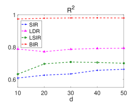
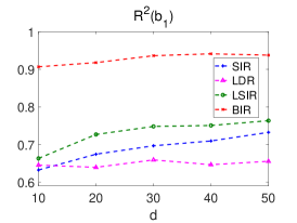
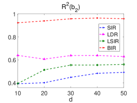
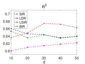
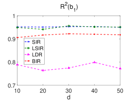
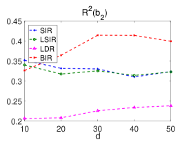
Figure 1: The $R^{2}$ accuracy of the DR subspace (left), the first DR direction $\mathbf{b}_{1}$ (center) and the second DR direction $\mathbf{b}_{2}$ (right), all plotted against the dimensionality. (a) results for function (4.2a); (b) results for function (4.2b).

4.1 Mathematical examples with increasing dimensions

First we consider a $d$-dimensional problem where $\mathbf{x}$ follows a standard normal distribution. The data are simulated from the following functions:

$$\quad f(\mathbf{x},\epsilon) =x_{1}(x_{2}+x_{3})+0.5\epsilon,$$ (4.2a)

$$\quad f(\mathbf{x},\epsilon) =\frac{x_{1}+x_{2}+x_{3}}{0.5+(x_{4}+x_{5})^{2}}+0.1\epsilon,$$ (4.2b)

where $\epsilon\sim N(0,1)$. Both problems have two DR directions. In the regression content, a well known limitation of the GP method is that it can not handle high dimension, and so here we want to test the scalability of the BIR method with respect to dimensionality. To do so we perform experiments for various dimensions: $d=10,\,20,\,30,\,40,\,50$, where we set the number of data points to be $n=5d$, i.e., growing linear with respect to dimensionality. To evaluate the performance of the methods, we use the $R^{2}$ metric of accuracy used in li1991sliced to measure the accuracy of the DR subspace and the DR directions.

We repeat all the tests for $100$ times and report the average. Specifically, we show the $R^{2}$-accuracy of the DR subspace $B$ and the two DR directions in Figs. 1. We can see that the BIR method has the best performance in all the tests in the two examples, except one situation: $d=10$ for function (4.2b). The $R^{2}$ accuracy for each DR direction provide more information on the results. Namely, for Function 4.2a, BIR performs better than all the other methods in both of the directions. For function 4.2b, the accuracy of BIR is slightly lower than than SIR and LSIR for the first direction, but it achieves significantly higher accuracy on the second dimension than all the other ones. Finally we want to note here that as the dimensionality increases, the performance of BIR does not decay evidently, suggesting that the method can handle rather high dimensional problems.

4.2 Mathematical examples with non Gaussian distributions

In our second example, we want to test the performance of the methods when the distribution of $\mathbf{x}$ is strongly non-Gaussian. We assume $\mathbf{x}$ is a 10-dimensional variable and the data are generated as follows. First let $\mathbf{u}=(u_{1},u_{2})$ follow a two-dimensional standard normal distribution. We then perform the following transform:

$$x_{1}=u_{1},\quad x_{2}=u_{1}-bu_{1}^{2},$$ (4.3)

where $b\geq 0$. Here by varying parameter $b$ one can control how different the distribution of $\mathbf{x}$ is from Gaussian. Data of $y$ are generated from $\mathbf{u}$, and so the transformation used to generating $\mathbf{x}$ does not affect the data of $y$. In this example we use the following two functions to generate $y$:

$$\quad y =\frac{u_{1}}{0.5+(u_{2}+1.5)^{2}}+0.5\epsilon,$$ (4.4a)

$$\quad y =\sin(5\pi u_{1})+u_{2}^{2}+0.1\epsilon,$$ (4.4b)

where $\epsilon\sim N(0,1)$. In this test, we choose five different values of $b$: $b=0,\,5,\,10,\,15,\,20$ with sample size $n=100$, and we show the scatter plots of the data points for all these cases in Fig. 2, where we can see that the resulting data points move apart from Gaussian as $b$ increases. We plot the $R^{2}$ accuracy against the value of $b$ in Figs. 3 for both functions. From the figures we can see that for function 4.4a, BIR clearly outperforms all the other methods for all the values of $b$, and for function 4.4b, the BIR also has the best performance in all the cases, with LDR being about the same at $b=10$ and $20$.

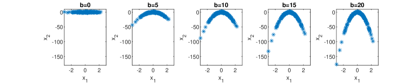
Figure 2: The scatter plots of $(x_{1},x_{2})$ for different values of $b$.

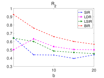
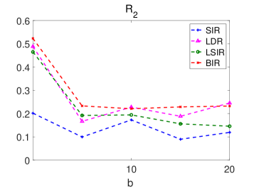
Figure 3: The $R^{2}$-accuracy of the DR subspace plotted as a function of $b$, for function (4.4a) (left) and function (4.4b) (right) respectively.

4.3 Mathematical example for BAVE

We now consider a mathematical example which requires to consider the 2nd moments. Let $\mathbf{x}$ be a 20 dimensional random variable following standard normal distribution, and let

$$y=x_{1}^{2}+0.1\epsilon,$$

where noise $\epsilon\sim\mathpzc{N}(0,1)$. It is easy to verify that $E(\mathbf{x}|y)=0$, which implies that the first moment based approach, i.e., SIR, does not apply to this problem.

We conduct numerical experiments with six different sample sizes: 30, 40, 60, 80, 100 and 120, and for each sample size, we randomly generate 100 sets of data. With each set of data, we estimate the DR direction with SIR, LDR, SAVE and BAVE. The $R^{2}$ accuracy of the DR direction obtained by each method, averaged over the 100 trials, is shown in Fig. 4. As expected, SIR fails completely for this example – its resulting $R^{2}$ accuracy is near zero, regardless of the sample size. The results of LDR are better than SIR but the overall accuracy remains quite low (less than $0.4$) even when the sample size reaches 120. On the other hand, the performance of SAVE and BAVE increases notably as the sample size increases, while for each sample size, the results of BAVE are considerably better than those of SAVE, suggesting that BAVE performs considerably better than SAVE for this small dataset problem.

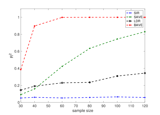
Figure 4: The $R^{2}$ accuracy of the DR direction computed with different same sizes.

4.4 Death rate prediction

Methods	$n=15$	$n=20$	$n=25$	$n=30$	$n=35$	$n=40$
w/o DR	$.1832$	$.0855$	$.0551$	$\mathbf{.0460}$	$\mathbf{.0425}$	$\mathbf{.0380}$
	$\left(.2013\right)$	$\left(.0502\right)$	$\left(.0216\right)$	$\left(.0171\right)$	$\left(.0161\right)$	$\left(.0089\right)$
LDR	-	$.0823$	$.0569$	$.0490$	$.0444$	$.0383$
	(-)	$\left(.0518\right)$	$\left(.0207\right)$	$\left(.0184\right)$	$\left(.0173\right)$	$\left(.0089\right)$
SIR	$.4403$	$.0982$	$.0653$	$.0548$	$.0525$	$.0430$
	$\left(1.2417\right)$	$\left(.0769\right)$	$\left(.0310\right)$	$\left(.0216\right)$	$\left(.0217\right)$	$\left(.0108\right)$
LSIR	-	$.0876$	$.0648$	$.0557$	$.0485$	$.0429$
	(-)	$\left(.0461\right)$	$\left(.0252\right)$	$\left(.0224\right)$	$\left(.0174\right)$	$\left(.0100\right)$
BIR	$\mathbf{.0484}$	$\mathbf{.0451}$	$\mathbf{.0465}$	$.0481$	$.0466$	$.0468$
	$\left(.0110\right)$	$\left(.0104\right)$	$\left(.0111\right)$	$\left(.0105\right)$	$\left(.0114\right)$	$\left(.0126\right)$

Table 1: The mean and the standard deviation (in parenthesis) of MRRE for Example 3. The best results are marked in bold.

Methods	min	max
w/o DR	$.0289$	$.3374$
LDR	$.0281$	$.7913$
SIR	$.0362$	$.2534$
LSIR	$.0380$	$.2350$
BIR	$\mathbf{.0247}$	$\mathbf{.1183}$

Table 2: The minimal and maximal relative regression error (RRE) in the 100 trials with 20 data points for the death rate example. The best results are marked in bold.

The example considered in this section is to use pollution and related factors to predict the death rate mcdonald1973instabilities ; chatterjee2015regression . This is a regression problem with 15 predictors and 60 data points and we choose this example to test how the methods perform with very small number of data. We first apply the DR methods to select one feature (we have conducted tests with 2 and 3 features which does not improve the regression accuracy, and so we omit those results here) and then construct a standard linear regression model of the data in the reduced dimension. As a comparison, we also perform the regression directly without DR. To test the methods with different numbers of data, we perform the experiments with $15$, $20$, $25$, $30$, $35$, $40$ data points randomly selected from the data set and another randomly selected 20 data points used as the test set. In each experiment we can compute the mean relative regression error (MRRE) using the data in the test set. Specifically, suppose $\{(\mathbf{x}_{i},y_{i})\}_{i=1}^{n_{t}}$ is the training set and $f_{r}(\cdot)$ is the regression model, the MRRE is computed as,

$$\mathrm{MRRE}=\frac{1}{n_{t}}\sum_{i=1}^{n_{t}}\frac{|y_{i}-f_{r}(\mathbf{x}_{i})|}{y_{i}}.$$

We repeat all the experiments 100 times, and compute the mean and the standard deviation of the obtained MRRE, which is shown in Table 1. First we observe that for $n=40$ all the methods can achieve rather good accuracy; as $n$ decrease, the results of all the other methods become evidently worse, while that of BIR remains quite stable, suggesting that the BIR is especially effective in the small data case. It should be noted that for $n=15$ LDR and LSIR fail to produce reasonable results due to numerical instability, and so we omit the results here. More importantly it can be seen from the table that starting from $n=30$, the regression without DR actually has the best performance, suggesting that implementing DR is only necessary when the number of data points is below 30. In all the cases DR is genuinely needed, i.e., $n<25$, the BIR method performs significantly better than all other methods. To further analyze the performance, we also compute the minimal and the maximal relative regression errors (RRE) for the 20 data-point case, and present the results in Table 2. Once again, we can see that the BIR method has the best results in both the minimal and the maximal cases.

sample size	$20$	$30$	$40$	$50$	$60$	$70$	$80$	$90$	$100$
w/o DR	$.377$	$.254$	$.210$	$.203$	$.181$	$.173$	$.173$	$.169$	$.170$
	$\left(.153\right)$	$\left(.072\right)$	$\left(.035\right)$	$\left(.0393\right)$	$\left(.025\right)$	$\left(.026\right)$	$\left(.022\right)$	$\left(.022\right)$	$\left(.022\right)$
LDR	$.394$	$.262$	$.209$	$.198$	$.178$	$.173$	$.175$	$.172$	$.171$
	$\left(.175\right)$	$\left(.097\right)$	$\left(.035\right)$	$\left(.033\right)$	$\left(.028\right)$	$\left(.031\right)$	$\left(.024\right)$	$\left(.027\right)$	$\left(.024\right)$
SIR	$.497$	$.284$	$.2358$	$.217$	$.199$	$.192$	$.193$	$.189$	$.187$
	$\left(.224\right)$	$\left(.093\right)$	$\left(.049\right)$	$\left(.044\right)$	$\left(.035\right)$	$\left(.034\right)$	$\left(.032\right)$	$\left(.030\right)$	$\left(.029\right)$
LSIR	$.489$	$.284$	$.225$	$.216$	$.194$	$.189$	$.190$	$.183$	$.178$
	$\left(.210\right)$	$\left(.079\right)$	$\left(.043\right)$	$\left(.040\right)$	$\left(.032\right)$	$\left(.034\right)$	$\left(.029\right)$	$\left(.033\right)$	$\left(.027\right)$
BIR	$\mathbf{.188}$	$.\mathbf{184}$	$\mathbf{.178}$	$\mathbf{.178}$	$\mathbf{.167}$	$\mathbf{.164}$	$\mathbf{.167}$	$\mathbf{.165}$	$\mathbf{.162}$
	$\left(.034\right)$	$\left(.034\right)$	$\left(.031\right)$	$\left(.029\right)$	$\left(.025\right)$	$\left(.027\right)$	$\left(.021\right)$	$\left(.024\right)$	$\left(.023\right)$

Table 3: The mean and the standard deviation (in parenthesis) of MRRE for Example 4. The best results are marked in bold.

Methods	min	max
w/o DR	$.1555$	$1.273$
LDR	$.170$	$1.134$
SIR	$.169$	$1.874$
LSIR	$.217$	$1.146$
BIR	$\mathbf{.113}$	$\mathbf{0.287}$

Table 4: The minimal and maximal relative regression error (RRE) in the 100 trials with 20 data points for the automobile price example. The best results are marked in bold.

4.5 Automobile data set

Our last example is the automobile data set in the UCI Machine Learning Repository Dua:2019 . The original data set contains 205 instances described by 26 attributes including 16 continuous and 10 categorical. We preprocess the data set in the following way: we neglect the 10 categorical attributes, and remove the instances with missing values, yielding a data set with 159 instances and 16 attributes. We select one of the 16 attributes as the response and the others as the predictors: specifically we want to predict the price of an automobile based the other 15 attributes of it. In this problem we first select one feature using the DR methods, and then perform a linear regression with the selected feature. Just like the previous example, we want to examine the performance of the DR methods in the small-data setting, i.e., a setting where direct regression can not provide accurate results. To do so, we conduct the experiments with $n=10,\,20,\,...,90,100$ randomly selected samples and another 50 random samples used as the test set for all the cases. We repeat each experiment 100 times, and compute the MRRE each time. The mean and the standard deviation of the MRRE results are reported in Table 3. From the data given in Table 3, we obtain rather similar conclusions as those of Example 3. Namely, the BIR method has the best MRRE of all the four methods used. In Table 4, we show the minimal and the maximal RRE for the 20 data-point case, and just like the results in Example 3, we find that the BIR method has the smallest RRE in both the minimal and the maximal cases.

5 Conclusions

We consider dimension reduction problems for regression and we propose a Bayesian approach for computing the conditional distribution $\pi(\mathbf{x}|y)$ and perform the dimension reduction. The method construct the likelihood function from the data with a GP regression model and MCMC to generate samples from the conditional distribution $\pi(\mathbf{x}|y)$. Numerical examples demonstrate that the proposed method is particularly effective for problems with very small data set. We reinstate here that, due to the use of GP model, BIR does not apply to problems with very high dimensions. Rather, we expect BIR can be useful for problems with moderately high dimensions, and a very limited amount of data.

We believe the method can be useful in many real world applications. For example, in many high dimensional inverse problems and data assimilation problems, one the data can only be informative on a small number of dimensions cui2014likelihood ; solonen2016dimension ; zahm2018certified . A method that utilizes the DR methods to identify such data informed dimensions is currently under investigation. On the other hand, in certain problems gradient information is available, and DR methods which takes advantages of the gradient information have also been developed, e.g. fukumizu2012gradient ; constantine2015active ; lam2018multifidelity . In this case, we expect that the gradient information can also be used to enhance the performance of the BIR method, via, for example, Gradient-Enhanced Kriging morris1993bayesian , and we plan to investigate this problem in the future.

References

- [1] Samprit Chatterjee and Ali S Hadi. Regression analysis by example. John Wiley & Sons, 2015.
- [2] Paul G Constantine. Active subspaces: Emerging ideas for dimension reduction in parameter studies, volume 2. SIAM, 2015.
- [3] R Dennis Cook and Liliana Forzani. Likelihood-based sufficient dimension reduction. Journal of the American Statistical Association, 104(485):197–208, 2009.
- [4] R Dennis Cook, Liliana M Forzani, and Diego R Tomassi. Ldr: A package for likelihood-based sufficient dimension reduction. Journal of Statistical Software, 39(i03), 2011.
- [5] R Dennis Cook and Liqiang Ni. Sufficient dimension reduction via inverse regression: A minimum discrepancy approach. Journal of the American Statistical Association, 100(470):410–428, 2005.
- [6] R Dennis Cook and Sanford Weisberg. Sliced inverse regression for dimension reduction: Comment. Journal of the American Statistical Association, 86(414):328–332, 1991.
- [7] Tiangang Cui, James Martin, Youssef M Marzouk, Antti Solonen, and Alessio Spantini. Likelihood-informed dimension reduction for nonlinear inverse problems. Inverse Problems, 30(11):114015, 2014.
- [8] R Dennis Cook. Save: a method for dimension reduction and graphics in regression. Communications in statistics-Theory and methods, 29(9-10):2109–2121, 2000.
- [9] Dheeru Dua and Casey Graff. UCI machine learning repository, 2017.
- [10] Louis Ferré. Determining the dimension in sliced inverse regression and related methods. Journal of the American Statistical Association, 93(441):132–140, 1998.
- [11] Kenji Fukumizu, Francis R Bach, and Michael I Jordan. Dimensionality reduction for supervised learning with reproducing kernel hilbert spaces. Journal of Machine Learning Research, 5(Jan):73–99, 2004.
- [12] Kenji Fukumizu and Chenlei Leng. Gradient-based kernel method for feature extraction and variable selection. In Advances in Neural Information Processing Systems, pages 2114–2122, 2012.
- [13] Minyoung Kim and Vladimir Pavlovic. Dimensionality reduction using covariance operator inverse regression. In 2008 IEEE Conference on Computer Vision and Pattern Recognition, pages 1–8. IEEE, 2008.
- [14] Rémi Lam, Olivier Zahm, Youssef Marzouk, and Karen Willcox. Multifidelity dimension reduction via active subspaces. arXiv preprint arXiv:1809.05567, 2018.
- [15] Bing Li. Sufficient dimension reduction: Methods and applications with R. CRC Press, 2018.
- [16] Bing Li, Yuexiao Dong, et al. Dimension reduction for nonelliptically distributed predictors. The Annals of Statistics, 37(3):1272–1298, 2009.
- [17] Bing Li and Shaoli Wang. On directional regression for dimension reduction. Journal of the American Statistical Association, 102(479):997–1008, 2007.
- [18] Ker-Chau Li. Sliced inverse regression for dimension reduction. Journal of the American Statistical Association, 86(414):316–327, 1991.
- [19] Lexin Li and Xiangrong Yin. Sliced inverse regression with regularizations. Biometrics, 64(1):124–131, 2008.
- [20] Qian Lin, Zhigen Zhao, and Jun S Liu. Sparse sliced inverse regression via lasso. Journal of the American Statistical Association, pages 1–33, 2019.
- [21] Yanyuan Ma and Liping Zhu. A semiparametric approach to dimension reduction. Journal of the American Statistical Association, 107(497):168–179, 2012.
- [22] Yanyuan Ma and Liping Zhu. A review on dimension reduction. International Statistical Review, 81(1):134–150, 2013.
- [23] Kai Mao, Feng Liang, and Sayan Mukherjee. Supervised dimension reduction using bayesian mixture modeling. In Proceedings of the Thirteenth International Conference on Artificial Intelligence and Statistics, pages 501–508, 2010.
- [24] Gary C McDonald and Richard C Schwing. Instabilities of regression estimates relating air pollution to mortality. Technometrics, 15(3):463–481, 1973.
- [25] Geoffrey McLachlan and David Peel. Finite Mixture Models. John Wiley & Sons, 2004.
- [26] Max D Morris, Toby J Mitchell, and Donald Ylvisaker. Bayesian design and analysis of computer experiments: use of derivatives in surface prediction. Technometrics, 35(3):243–255, 1993.
- [27] Brian J Reich, Howard D Bondell, and Lexin Li. Sufficient dimension reduction via bayesian mixture modeling. Biometrics, 67(3):886–895, 2011.
- [28] Antti Solonen, Tiangang Cui, Janne Hakkarainen, and Youssef Marzouk. On dimension reduction in gaussian filters. Inverse Problems, 32(4):045003, 2016.
- [29] Kean Ming Tan, Zhaoran Wang, Tong Zhang, Han Liu, and R Dennis Cook. A convex formulation for high-dimensional sparse sliced inverse regression. Biometrika, 105(4):769–782, 2018.
- [30] Surya T Tokdar, Yu M Zhu, Jayanta K Ghosh, et al. Bayesian density regression with logistic gaussian process and subspace projection. Bayesian analysis, 5(2):319–344, 2010.
- [31] Christopher KI Williams and Carl Edward Rasmussen. Gaussian processes for machine learning. MIT Press, 2006.
- [32] Qiang Wu, Sayan Mukherjee, and Feng Liang. Localized sliced inverse regression. In Advances in neural information processing systems, pages 1785–1792, 2009.
- [33] Yingcun Xia, Howell Tong, Wai Keungxs Li, and Li-Xing Zhu. An adaptive estimation of dimension reduction space. Journal of the Royal Statistical Society: Series B (Statistical Methodology), 64(3):363–410, 2002.
- [34] Xiangrong Yin and R Dennis Cook. Estimating central subspaces via inverse third moments. Biometrika, 90(1):113–125, 2003.
- [35] Olivier Zahm, Tiangang Cui, Kody Law, Alessio Spantini, and Youssef Marzouk. Certified dimension reduction in nonlinear bayesian inverse problems. arXiv preprint arXiv:1807.03712, 2018.
- [36] Li-Ping Zhu and Li-Xing Zhu. On kernel method for sliced average variance estimation. Journal of Multivariate Analysis, 98(5):970–991, 2007.